UNIVERSIDADE FEDERAL DO PARÁ

INSTITUTO DE TECNOLOGIA

PROGRAMA DE PÓS-GRADUAÇÃO EM ENGENHARIA ELÉTRICA

TÍTULO DO TRABALHO

Técnicas de Balanceamento de Taxas de Downstream

para Sistemas Vetorizados de Linha Digital do

Assinante (DSL): Estudo de Caso do Padrão ITU

G.9700

NOME DO AUTOR

Claudio de Castro Coutinho Filho

DM:11/2015

UFPA / ITEC / PPGEECampus Universitário do Guamá

Belém-Pará-Brasil2015

II

FEDERAL UNIVERSITY OF PARÁ

INSTITUTE OF TECHNOLOGY

GRADUATE PROGRAM ON ELECTRICAL ENGINEERING

TITLE

Techniques of Downstream Rate Balancing for

Vectored Digital Subscriber Line Systems: Case Study

of the ITU G.9700 Standard

AUTHOR

Claudio de Castro Coutinho Filho

DM:11/2015

UFPA / ITEC / PPGEECampus Universitário do Guamá

Belém-Pará-Brazil2015

III

FEDERAL UNIVERSITY OF PARÁ

INSTITUTE OF TECHNOLOGY

GRADUATE PROGRAM ON ELECTRICAL ENGINEERING

TITLE

Techniques of Downstream Rate Balancing for

Vectored Digital Subscriber Line Systems: Case Study

of the ITU G.9700 Standard

AUTHOR

Claudio de Castro Coutinho Filho

A dissertation submitted to the Exam-

ining Board of the Graduate Program

on Electrical Engineering from UFPA

for obtaining the degree of Master of

Science on Electrical Engineering, em-

phasis on Telecommunications.

UFPA / ITEC / PPGEECampus Universitário do Guamá

Belém-Pará-Brazil2015

IV

Dados Internacionais de Catalogação-na-Publicação (CIP)Sistema de Bibliotecas da UFPA

Coutinho Filho, Claudio de Castro, 1989-Techniques of Downstream Rate Balancing for Vectored Digital Subscriber Line

Systems: Case Study of the ITU G.9700 Standard/ Claudio de Castro Coutinho Filho. -

2015.Orientador: Aldebaro Barreto da Rocha

Klautau Jr..Dissertação (Mestrado) - Universidade

Federal do Pará, Instituto de Tecnologia,Programa de Pós-Graduação em EngenhariaElétrica, Belém, 2015.

1. Modem. 2. Algoritmo genético. I. Título.CDD 22. ed. 621.39814

V

UNIVERSIDADE FEDERAL DO PARÁ

INSTITUTO DE TECNOLOGIA

PROGRAMA DE PÓS-GRADUAÇÃO EM ENGENHARIA ELÉTRICA

Techniques of Downstream Rate Balancing for Vectored Digital SubscriberLine Systems: Case Study of the ITU G.9700 Standard

AUTOR: Claudio de Castro Coutinho Filho

DISSERTAÇÃO DE MESTRADO SUBMETIDA À AVALIAÇÃO DA BANCA EXAMINADORA

APROVADA PELO COLEGIADO DO PROGRAMA DE PÓS-GRADUAÇÃO EM ENGENHARIA

ELÉTRICA, SENDO JULGADA ADEQUADA PARA A OBTENÇÃO DO GRAU DE MESTRE EM

ENGENHARIA ELÉTRICA NA ÁREA DE TELECOMUNICAÇÕES.

APROVADA EM 10/03/2015

BANCA EXAMINADORA:

.................................................................................................

Prof. Dr. Aldebaro Barreto da Rocha Klautau Júnior (ORIENTADOR - UFPA)

.................................................................................................

Prof. Dr. Ádamo Lima de Santana (MEMBRO - UFPA)

.................................................................................................

Prof. Dr. Claudomiro de Souza de Sales Junior (MEMBRO - UFPA)

.................................................................................................

Prof. Dr. Francisco Carlos Bentes Frey Muller (MEMBRO - UFPA)

.................................................................................................

Prof. Dr. Bruno Souza Lyra Castro (MEMBRO - IESAM)

VISTO:

.................................................................................................

Prof.a Dr.a Maria Emília de Lima Tostes

Vice-Coordenadora do PPGEE/ITEC/UFPA

VI

Acknowledgements

I would like to show recognition to all those who contributed to the realization of

this Master’s Dissertation work.

I thank my family for their understanding in moments of absence and unavailability.

I thank my friends, always encouraging and giving strength in the most difficult

moments of this stage.

I thank the friends from LaPS, always willing to help the smallest detail and to

provide moments of relaxation and leisure.

I thank my beloved friend, partner, Bianca, who has been the basis of all my

motivation to get where I am.

I thank my advisor, Prof. Aldebaro Klautau Jr, for all the assistance provided and

the knowledge conceived throughout this learning process.

And I thank all those who support the scientific curiosity and contribute to open

the doors of knowledge to everyone, so that the flame of wisdom never extinguishes.

Claudio de Castro Coutinho Filho

VII

Contents

1 INTRODUCTION 1

1.1 Motivation . . . . . . . . . . . . . . . . . . . . . . . . . . . . . . . . . . . . 1

1.2 Rate-balancing . . . . . . . . . . . . . . . . . . . . . . . . . . . . . . . . . 2

1.3 Structure of the work . . . . . . . . . . . . . . . . . . . . . . . . . . . . . . 3

2 THEORETICAL BASIS 5

2.1 MIMO . . . . . . . . . . . . . . . . . . . . . . . . . . . . . . . . . . . . . . 5

2.2 G.fast . . . . . . . . . . . . . . . . . . . . . . . . . . . . . . . . . . . . . . 6

2.3 Gram-Schmidt . . . . . . . . . . . . . . . . . . . . . . . . . . . . . . . . . . 9

2.4 QR Decomposition . . . . . . . . . . . . . . . . . . . . . . . . . . . . . . . 11

2.4.1 Matrix representation . . . . . . . . . . . . . . . . . . . . . . . . . . 11

2.4.2 Decomposition using Gram-Schmidt . . . . . . . . . . . . . . . . . . 12

2.5 Vectoring . . . . . . . . . . . . . . . . . . . . . . . . . . . . . . . . . . . . 13

2.5.1 Precoder matrix . . . . . . . . . . . . . . . . . . . . . . . . . . . . . 13

2.5.2 Linear Precoder . . . . . . . . . . . . . . . . . . . . . . . . . . . . . 14

2.5.2.1 System model . . . . . . . . . . . . . . . . . . . . . . . . . 15

2.5.2.2 The Diagonalizing Precoder . . . . . . . . . . . . . . . . . 16

2.5.3 The Tomlinson-Harashima Precoder . . . . . . . . . . . . . . . . . . 19

3 RATE-BALANCING TECHNIQUES 27

VIII

3.1 GS-Sorting . . . . . . . . . . . . . . . . . . . . . . . . . . . . . . . . . . . . 29

3.2 Post-sorting . . . . . . . . . . . . . . . . . . . . . . . . . . . . . . . . . . . 30

3.3 Original Sorting . . . . . . . . . . . . . . . . . . . . . . . . . . . . . . . . . 31

3.4 Genetic Algorithm Sorting . . . . . . . . . . . . . . . . . . . . . . . . . . . 32

3.4.1 Structure . . . . . . . . . . . . . . . . . . . . . . . . . . . . . . . . 32

3.4.2 Crossover . . . . . . . . . . . . . . . . . . . . . . . . . . . . . . . . 33

3.4.3 Fitness function . . . . . . . . . . . . . . . . . . . . . . . . . . . . . 34

3.4.4 Algorithm . . . . . . . . . . . . . . . . . . . . . . . . . . . . . . . . 35

4 RESEARCH RESULTS 37

4.1 Simulated cables . . . . . . . . . . . . . . . . . . . . . . . . . . . . . . . . 37

4.1.1 Row-wise Diagonal Dominance . . . . . . . . . . . . . . . . . . . . 39

4.1.2 Near-Far scenario . . . . . . . . . . . . . . . . . . . . . . . . . . . . 40

4.1.3 Comparison rates . . . . . . . . . . . . . . . . . . . . . . . . . . . . 41

4.1.3.1 BT cable . . . . . . . . . . . . . . . . . . . . . . . . . . . 42

4.1.3.2 DT cable . . . . . . . . . . . . . . . . . . . . . . . . . . . 43

4.1.3.3 Ericsson cable . . . . . . . . . . . . . . . . . . . . . . . . . 44

4.1.3.4 Swisscom PE4D cable . . . . . . . . . . . . . . . . . . . . 46

4.1.3.5 Swisscom I51 cable . . . . . . . . . . . . . . . . . . . . . . 47

4.1.3.6 Swisscom P-ALT cable . . . . . . . . . . . . . . . . . . . . 48

4.1.4 Overall results . . . . . . . . . . . . . . . . . . . . . . . . . . . . . . 50

5 CONCLUSION AND FURTHER WORKS 52

BIBLIOGRAPHY 54

IX

List of Figures

1.1 DSL ports using Vectoring annually. Source: [1]. . . . . . . . . . . . . . . . 2

2.1 Different kinds of MIMO techniques. Source: [2]. . . . . . . . . . . . . . . . 6

2.2 Representation of the MIMO basic relation y = Hx + n. . . . . . . . . . . 7

2.3 Increase of bandwidth with G.fast. Source: [3]. . . . . . . . . . . . . . . . . 8

2.4 Illustration of different fiber-to-the-x architectures. Source: [4]. . . . . . . . 9

2.5 Relation between vectors in GS-decomposition. . . . . . . . . . . . . . . . . 9

2.6 Achievable rates using Vectoring. Source: [5]. . . . . . . . . . . . . . . . . . 13

2.7 Comparison between precoders. . . . . . . . . . . . . . . . . . . . . . . . . 14

2.8 FEXT caused by line 1 on line 2. . . . . . . . . . . . . . . . . . . . . . . . 16

2.9 Diagram representing the role played by the DP. . . . . . . . . . . . . . . . 17

2.10 Comparison between transmissions with and without DP. . . . . . . . . . . 19

2.11 Modulo function bounding the values of x′𝑘 with 200 symbols. . . . . . . . 25

2.12 Diagram of the precoding process. . . . . . . . . . . . . . . . . . . . . . . . 25

3.1 Penalization of last lines. . . . . . . . . . . . . . . . . . . . . . . . . . . . . 28

3.2 Column sorting for achieving rate-balancing. . . . . . . . . . . . . . . . . . 28

3.3 Chromosome’s structure for a 10-line cable. . . . . . . . . . . . . . . . . . . 32

3.4 Crossover of two parent chromosomes. . . . . . . . . . . . . . . . . . . . . 33

3.5 Illustration of the Mutation process. . . . . . . . . . . . . . . . . . . . . . . 33

3.6 Fitness function in relation to 𝜎𝑘 and bitload. . . . . . . . . . . . . . . . . 34

X

3.7 Fitness values for 100 generations. . . . . . . . . . . . . . . . . . . . . . . . 35

4.1 Row-wise Diagonal Dominance for each worked cable. . . . . . . . . . . . . 40

4.2 Representation of the Near-Far scenario with 4 lines. . . . . . . . . . . . . 41

4.3 British Telecom cable rates. . . . . . . . . . . . . . . . . . . . . . . . . . . 42

4.4 Deutsche Telekom I-Y(ST)Y cable rates. . . . . . . . . . . . . . . . . . . . 44

4.5 Ericsson cable rates. . . . . . . . . . . . . . . . . . . . . . . . . . . . . . . 45

4.6 Swisscom PE4D cable rates. . . . . . . . . . . . . . . . . . . . . . . . . . . 46

4.7 Swisscom I51 cable rates. . . . . . . . . . . . . . . . . . . . . . . . . . . . . 48

4.8 Swisscom P-ALT cable rates. . . . . . . . . . . . . . . . . . . . . . . . . . 49

4.9 Impact of RWDD on the rate-balancing methods’ performance. . . . . . . . 50

XI

List of Tables

3.1 GA parameters. . . . . . . . . . . . . . . . . . . . . . . . . . . . . . . . . . 35

4.1 Cables used in all simulations . . . . . . . . . . . . . . . . . . . . . . . . . 38

4.2 BT cable rates. . . . . . . . . . . . . . . . . . . . . . . . . . . . . . . . . . 43

4.3 DT I-Y(ST)Y cable rates. . . . . . . . . . . . . . . . . . . . . . . . . . . . 43

4.4 Ericsson cable rates. . . . . . . . . . . . . . . . . . . . . . . . . . . . . . . 45

4.5 Swisscom PE4D cable rates. . . . . . . . . . . . . . . . . . . . . . . . . . . 47

4.6 Swisscom I51 cable rates. . . . . . . . . . . . . . . . . . . . . . . . . . . . . 48

4.7 Swisscom P-ALT cable rates. . . . . . . . . . . . . . . . . . . . . . . . . . 49

Abbreviations

4GBB Fourth Generation BroadBand

AWGN Additive White Gaussian Noise

BT British Telecom

CO Central Office

CPE Customer Premises Equipment

CWDD Column-wise Diagonal Dominance

DP Diagonalizing Precoder

DSL Digital Subscriber Line

DSLAM Digital Subscriber Line Access Multiplexer

DT Deutsche Telekom

FEQ Frequency Domain Equalizer

FEXT Far-End Crosstalk

FTTX Fiber-to-the-x

GA Genetic Algorithm

XII

XIII

Gbps Gigabits per seconds

GS Gram-Schmidt

ISP Internet Service Provider

ITU International Telecommunication Union

ITU-T ITU - Telecommunication Standardization Sector

Mbps Megabits per second

MIMO Multiple-Input Multiple-Output

MIPS Millions of Instructions Per Second

MISO Multiple-Input Single-Output

QAM Quadrature Amplitude Modulation

QoS Quality of Service

RFI Radio Frequency Interference

RWDD Row-wise Diagonal Dominance

SIMO Single-Input Multiple-Output

SISO Single-Input Single-Output

SNR Signal-to-Noise Ratio

THP Tomlinson-Harashima Precoder

XIV

Resumo

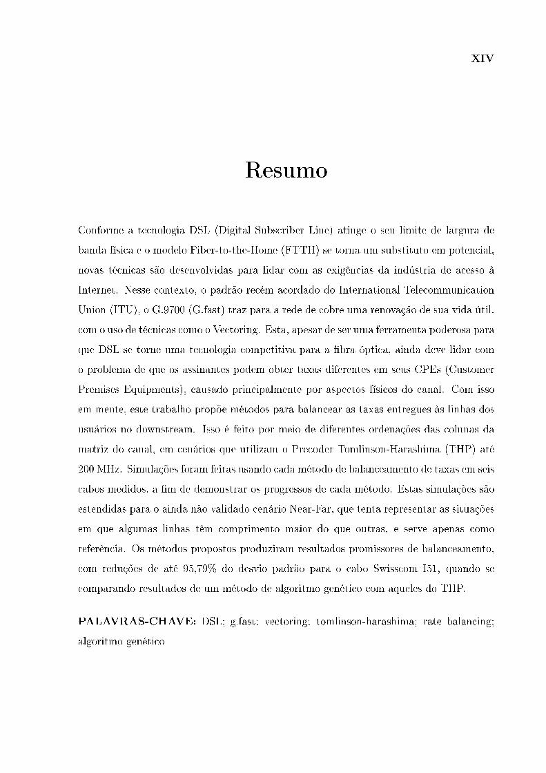
Conforme a tecnologia DSL (Digital Subscriber Line) atinge o seu limite de largura de

banda física e o modelo Fiber-to-the-Home (FTTH) se torna um substituto em potencial,

novas técnicas são desenvolvidas para lidar com as exigências da indústria de acesso à

Internet. Nesse contexto, o padrão recém acordado do International Telecommunication

Union (ITU), o G.9700 (G.fast) traz para a rede de cobre uma renovação de sua vida útil,

com o uso de técnicas como o Vectoring. Esta, apesar de ser uma ferramenta poderosa para

que DSL se torne uma tecnologia competitiva para a fibra óptica, ainda deve lidar com

o problema de que os assinantes podem obter taxas diferentes em seus CPEs (Customer

Premises Equipments), causado principalmente por aspectos físicos do canal. Com isso

em mente, este trabalho propõe métodos para balancear as taxas entregues às linhas dos

usuários no downstream. Isso é feito por meio de diferentes ordenações das colunas da

matriz do canal, em cenários que utilizam o Precoder Tomlinson-Harashima (THP) até

200 MHz. Simulações foram feitas usando cada método de balanceamento de taxas em seis

cabos medidos, a fim de demonstrar os progressos de cada método. Estas simulações são

estendidas para o ainda não validado cenário Near-Far, que tenta representar as situações

em que algumas linhas têm comprimento maior do que outras, e serve apenas como

referência. Os métodos propostos produziram resultados promissores de balanceamento,

com reduções de até 95,79% do desvio padrão para o cabo Swisscom I51, quando se

comparando resultados de um método de algoritmo genético com aqueles do THP.

PALAVRAS-CHAVE: DSL; g.fast; vectoring; tomlinson-harashima; rate balancing;

algoritmo genético

XV

Abstract

As the DSL (Digital Subscriber Line) technology reaches its physical bandwidth limit and

the Fiber-to-the-Home (FTTH) model becomes a potential substitute, new techniques and

standards are developed to cope with the requirements from the Internet access indus-

try. In this context, the newly agreed G.9700 (G.fast) standard, from the International

Telecommunication Union (ITU), brings to the copper plant a renewal of its lifespan with

the use of techniques such as Vectoring. Although Vectoring is a powerful tool for DSL

to become a competitive technology for optical fiber, it must deal with the problem that

subscribers still may get differing rates at their CPEs (Customer Premises Equipment),

caused mainly by physical aspects of the channel. With that in mind, this work proposes

methods of balancing the achievable rates delivered to user lines at Downstream. This is

done by using different column sortings of the channel matrix, in scenarios that utilize the

Tomlinson-Harashima Precoder (THP) up to 200 MHz. Simulations using each rate bal-

ancing method on six measured cables are made in order to show each method’s progress.

These simulations are extended to the Near-Far Scenario, which tries to resemble the

situations where some lines have greater length than others, that is, differing distances

between the CPE and the DSLAM (Digital Subscriber Line Access Multiplexer). The

proposed methods yielded promising balancing result, with reductions of up to 95.79% of

the standard deviation for the Swisscom I51 cable, when comparing results of a genetic

algorithm method with those of the THP.

KEYWORDS: DSL; g.fast; vectoring; tomlinson-harashima; rate balancing; genetic

algorithm

Chapter 1

INTRODUCTION

Since the beginning of the 20th century, telecommunication systems have always

been changing. New inventions, devices, machinery, techniques come up every day in an

unstoppable rush. This is due to the importance and impact this branch of engineering

has on consumers’ lives. Personal computers, mobile phones, smart televisions and many

other devices are more and more connecting to each other through the global network.

This huge need for information brings along the need for more capacity and data rates

from the service providers. The motivation of this work is conceived from this scenario

and is presented in the next section.

1.1 MOTIVATION

As we are going to see in the next chapters, the new inventions in the field of

technology are accompanied by several adversities, such as interference, crosstalk and

many others. To address these problems or at least try to diminish their impact, some

techniques have been developed deployed in many telecommunication systems in private

or public networks. From this point, a new concept is conceived: "Vectoring", that is, a

set of techniques capable of effectively cancelling crosstalk [6], in order to provide better

service quality and data transmission. The term "Vectoring" is used to describe the

definitions of the ITU G.Vector standard [7]. The Vectoring techniques have started to

1

2

Figure 1.1: DSL ports using Vectoring annually. Source: [1].

be implemented in the commercial networks in some parts of the globe and it will possibly

be in focus in the next years, thus all methods used by Vectoring to expand its efficiency

(such as mathematical operations) will surely be explored and researched. Figure 1.1

demonstrates how the use of Vectoring has expanded in the recent years, at least when

using VDSL2. As of 2017, more than 50,000 DSL Ports are expected to receive Vectored

VDSL2. With that in mind, this work was conceived from the idea that the Vectoring

research field has a huge potential and must broadened, considering not only crosstalk

cancelling, but aspects that may impact the end-user experience while hiring the ISP

services. One of these aspects are the rate-balancing techniques.

1.2 RATE-BALANCING

One of the most important structures in the Vectoring field is the so-called precoder

matrix. In a DSL transmission system, this structure is responsible for adding complexity

to transmitted data prior to its transmission, trying to surpass the Far-End-Crosstalk

(FEXT), i.e., the crosstalk that each line causes on the other lines at the far end of the

cable, with respect to the interfering transmitter. The first release of G.fast determines

3

that, up to 100 MHz, the kind of precoder to be used is the one that implements lin-

ear operations for cancelling crosstalk. However, as the frequency increases, the Linear

Precoder, or Diagonalizing Precoder (DP), becomes unstable. In this scenario, a poten-

tial substitute is the Tomlinson-Harashima Precoder (THP). This precoding structure

uses nonlinear operations to perform crosstalk cancelling, such as the modulo operation.

That means an increase of data that can be delivered when setting frequency limits up

to 200 MHz. Although the THP appears as a promising solution, the nature of its im-

plementation brings some limitations. As it will be shown, these limitations, caused by

mathematical aspects, may affect the data delivered to subscribers, causing some of them

to receive more or less data than the others. For that matter, this work introduces the

rate-balancing methods, or techniques. As their name already attests, these techniques

try to balance the bitrates among users (or lines) in the same binder at their Customer

Premises Equipments (CPEs), by altering the order in which they are processed at the

Central Office (CO). This sorting is able to achieve a good approximation among lines

taking into account many factors, such as the norms of each column in the channel ma-

trix. These are the focus of this work, by proposing methods that try to diminish the

difference among lines, by setting parameters to be calculated starting from the channel

matrix. Likewise, a genetic algorithm sorting method is proposed to search for the best

possible sorting that can get closer to the optimal solution, by minimizing the total bi-

trate variance of all lines and maximizing the total bitrate sum. This can be a convenient

tool for a proper comparison between each method and the optimal achieved results for

testing their performance.

The search for the optimum could be easily done by simply testing each possible

line sorting in the channel matrix, however, some cables gather information for up to

24 lines, making it a 6.2045 × 1023 (24!) sample space, what would eventually cause the

computer to run out of memory.

1.3 STRUCTURE OF THE WORK

The chapters in this work try to provide the reader with a better understanding

of the foundations in the field of MIMO, and specifically in the field of Vectoring, so that

4

all concepts and theories here presented do not face any loophole that could make the

understanding unclear. With this in mind, the chapters are organized as follows:

Chapter 1 introduces the reader to the context where Vectoring is studied. The

motivations that led the research to seek new ways to increase data rates with the high

performance G.fast standard and how the proposed methods apply to what has been

conceived in Vectoring so far.

Chapter 2 talks about basic concepts that will be necessary if the reader is looking

for a clear understanding of how the proposed methods work. Concepts like MIMO, G.fast

and Vectoring are presented and explained for a better reading throughout this work.

The main work comes in Chapter 3, where the proposed rate-balancing methods

are discussed in the mathematical level, starting from the basic theory to the top-level

algorithms developed in the course of this research.

In Chapter 4, all simulations results come together to show how the proposed

methods work in comparison to different scenarios by showing the bitrates achieved by

each one.

The final chapter (5) aims at assembling all information presented in the previ-

ous chapters and sets the basis for further researches that will be made in the topic of

Vectoring.

Chapter 2

THEORETICAL BASIS

For a better understanding of the main concepts that will be used throughout

this work, it is desirable for the reader to be comfortable with the theoretical foundation

necessary for a whole comprehension. With that in mind, this chapter starts by explaining

the basics of MIMO, since it is where the Vectoring theory is based on. This chapter also

addresses the basic concepts of G.fast – the ITU-T standard that defines the background

parameters for this research.

2.1 MIMO

Acronym for Multiple-Input Multiple-Output, MIMO is the generalization of meth-

ods that imply the usage of multiple antennas both at the transmitter and the receiver for

exploiting the benefits of multipath propagation [8] and it has been part of communication

standards such as IEEE 802.11n [9]. The term MIMO also describes techniques derived

from its main idea of multipath propagation, where either the transmitter or the receiver

have different numbers of antennas (from one to many). Such techniques are known as

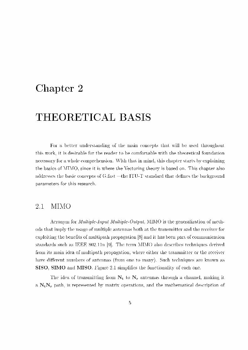
SISO, SIMO and MISO. Figure 2.1 simplifies the functionality of each one.

The idea of transmitting from Nt to Nr antennas through a channel, making it

a NtNr path, is represented by matrix operations, and the mathematical description of

5

6

Figure 2.1: Different kinds of MIMO techniques. Source: [2].

MIMO is given by

y = Hx + n, (2.1)

where y𝑁𝑟×1, x𝑁𝑡×1 and n𝑁𝑟×1 are the vectors containing the received samples, the trans-

mitted samples and the noise samples, respectively, and H𝑁𝑟×𝑁𝑡 is the channel matrix.

This relation is demonstrated in Figure 2.2.

2.2 G.FAST

Looking back at the history of internet services, especially in the post-dial-up era,

the increasingly huge need for data has always been a concern for the industry. Even more

people having access to the worldwide web compels the ISPs to meet these requirements.

After the advent of ADSL and later VDSL, the expectations for optic fiber de-

ployments grow every day, so it would not be wrong to think of fiber as the successor for

VDSL, due to its capacity to deliver high data rates to subscribers. However, as pointed

by Ödling et al. [10], there is a gap between these two so-called generations, a gap named

7

Figure 2.2: Representation of the MIMO basic relation y = Hx + n.

as the "fourth generation", conceptualized by the 4GBB project. The main aspect regard-

ing this generation is the economic feasibility of Fiber-to-the-Home deployment, that is,

the path between the CO and the CPE consisting solely of fiber loops. This concern gives

place to the possibility of achieving up to 1 Gbit/s rates using the existing copper plants

inside the residential and/or commercial establishments, reducing the need for digging

and installation procedures, for instance.

The "G.fast" denomination is a recursive acronym for fast access to subscriber

terminals and is dictated by the ITU-T documents G.9700 [11] and G.9701 [12]. It

is also referred to as an FTTdp (fiber-to-the-last-distribution-point) system, where the

DSLAMs (DSL access multiplexers) are located in the last distribution point in the copper

loop, up to 250 meters away from the end users. Such distance allows performances in

the range from 150 Mbit/s and 1 Gbit/s in contrast to VDSL2, that supports loops of up

to 2500 m [13]. This happens due to the bandwidth increase provided by G.fast, up to

212 MHz, as shown in Figure 2.3.

8

Figure 2.3: Increase of bandwidth with G.fast. Source: [3].

This increase of bandwidth forces the bitload limit down to 12 bits, to keep imple-

mentation complexity manageable. VDSL2 carries up to 15 bits per tone [14].

Speaking of performance, Telekom Austria and Alcatel-Lucent have already

achieved rates of 1.1 Gbit/s in laboratory, using a single line (not considering interference),

by a distance of 70 m [14] and first deployments of G.fast are expected for 2016 [15].

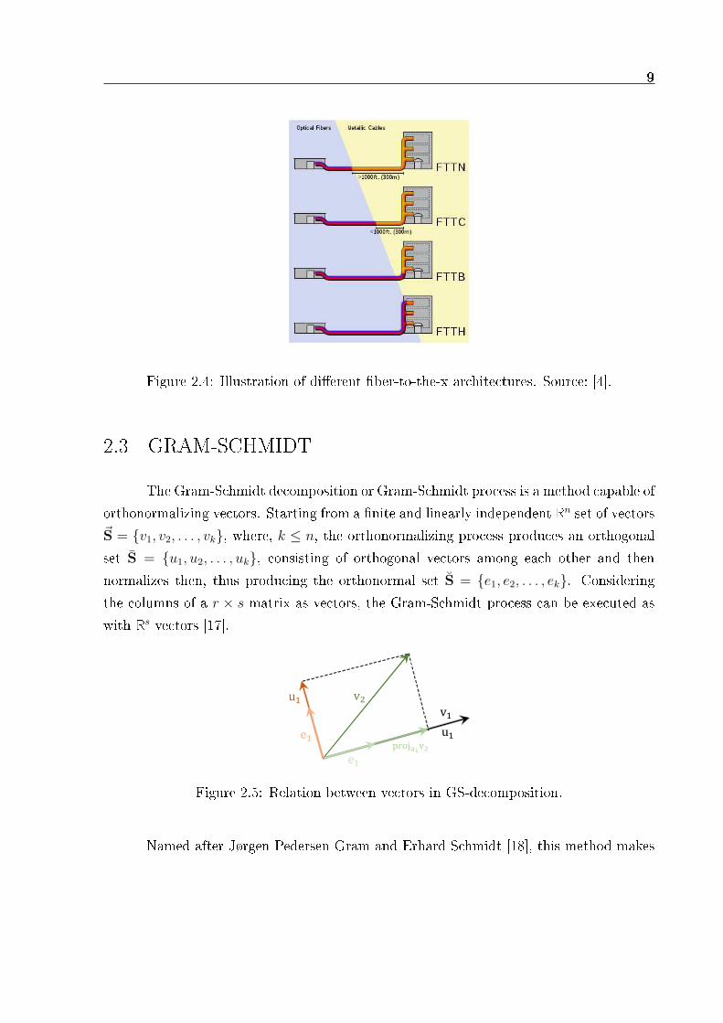
2.2.1 Fiber-to-the-x

The term "Fiber-to-the-x" is a generalization for several configurations of fiber de-

ployment. The main modalities are Fiber-to-the-Node, Fiber-to-the-Curb, Fiber-

to-the-Building, Fiber-to-the-last-distribution-point and finally Fiber-to-the-

Home, each one representing the length of existing copper that will be used, as demon-

strated in Figure 2.4.

One of the modalities usually associated to G.fast is Fiber-to-the-distribution-

point (FTTdp), similarly to VDSL2, which was associated to FTTN. In this modality,

the G.fast FTTdp fiber node has the approximate size of a large shoebox and can be

mounted on a pole or underground [16].

9

Figure 2.4: Illustration of different fiber-to-the-x architectures. Source: [4].

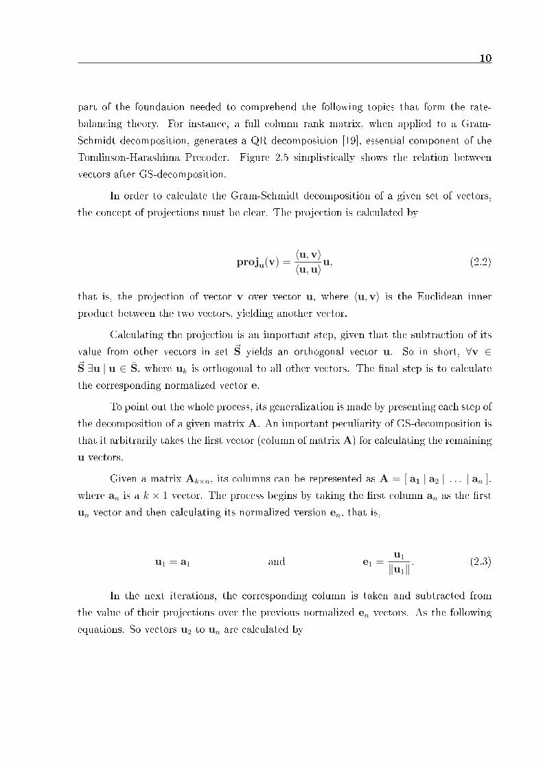
2.3 GRAM-SCHMIDT

The Gram-Schmidt decomposition or Gram-Schmidt process is a method capable of

orthonormalizing vectors. Starting from a finite and linearly independent R𝑛 set of vectors

S = {𝑣1, 𝑣2, . . . , 𝑣𝑘}, where, 𝑘 ≤ 𝑛, the orthonormalizing process produces an orthogonal

set S = {𝑢1, 𝑢2, . . . , 𝑢𝑘}, consisting of orthogonal vectors among each other and then

normalizes then, thus producing the orthonormal set S = {𝑒1, 𝑒2, . . . , 𝑒𝑘}. Considering

the columns of a 𝑟 × 𝑠 matrix as vectors, the Gram-Schmidt process can be executed as

with R𝑠 vectors [17].

Figure 2.5: Relation between vectors in GS-decomposition.

Named after Jørgen Pedersen Gram and Erhard Schmidt [18], this method makes

10

part of the foundation needed to comprehend the following topics that form the rate-

balancing theory. For instance, a full column rank matrix, when applied to a Gram-

Schmidt decomposition, generates a QR decomposition [19], essential component of the

Tomlinson-Harashima Precoder. Figure 2.5 simplistically shows the relation between

vectors after GS-decomposition.

In order to calculate the Gram-Schmidt decomposition of a given set of vectors,

the concept of projections must be clear. The projection is calculated by

proju(v) =⟨u,v⟩⟨u,u⟩

u, (2.2)

that is, the projection of vector v over vector u, where ⟨u,v⟩ is the Euclidean inner

product between the two vectors, yielding another vector.

Calculating the projection is an important step, given that the subtraction of its

value from other vectors in set S yields an orthogonal vector u. So in short, ∀v ∈S ∃u | u ∈ S, where u𝑘 is orthogonal to all other vectors. The final step is to calculate

the corresponding normalized vector e.

To point out the whole process, its generalization is made by presenting each step of

the decomposition of a given matrix A. An important peculiarity of GS-decomposition is

that it arbitrarily takes the first vector (column of matrixA) for calculating the remaining

u vectors.

Given a matrix A𝑘×𝑛, its columns can be represented as A = [ a1 | a2 | . . . | a𝑛 ],

where a𝑛 is a 𝑘 × 1 vector. The process begins by taking the first column a𝑛 as the first

u𝑛 vector and then calculating its normalized version e𝑛, that is,

u1 = a1 and e1 =u1

‖u1‖. (2.3)

In the next iterations, the corresponding column is taken and subtracted from

the value of their projections over the previous normalized e𝑛 vectors. As the following

equations. So vectors u2 to u𝑛 are calculated by

11

u2 = a2 − proje1(a2) and e2 =u2

‖u2‖, (2.4)

u3 = a3 − proje1(a3)− proje2(a3) and e3 =u3

‖u3‖. (2.5)

Thus, the generalized relation stands for

u𝑛 = a𝑛 −𝑛−1∑𝑗=1

proje𝑗(a𝑛) and e𝑛 =u𝑛

‖u𝑛‖. (2.6)

At the end of the process, 𝑛 orthogonal vectors u are obtained, as well as the

orthonormal e vectors (orthogonal with unit norm). Therefore,

u1⊥u2⊥ . . .⊥u𝑛 and ‖e1‖ = ‖e2‖ = · · · = ‖e𝑛‖ = 1. (2.7)

2.4 QR DECOMPOSITION

The QR decomposition, also known as QR factorization, is a process that takes a

matrix A as input and yields two other matrices: Q and R, forming the basic relation

A = QR, where Q is an orthogonal matrix, i.e. Q𝑇Q = I and R is an upper-triangular

matrix.

Regarded as the most important algorithmic idea in numerical linear algebra [20],

the QR decomposition serves as basis for several methods in the field of linear algebra,

such as the QR-algorithm, for computing eigenvalues [21] [22], considered one of the most

important algorithms of the twentieth century [23].

2.4.1 Matrix representation

Assuming a full column rank matrix A ∈ C𝑚×𝑛 (𝑚 ≥ 𝑛), and each column of

matrix A as a column vector a𝑛, and extending this notation for both Q (q𝑛) and R

(r𝑛𝑛) matrices, the resulting structure derived from the QR decomposition relation is

12

⎡⎢⎢⎢⎣ a1 a2 . . . a𝑛

⎤⎥⎥⎥⎦ =

⎡⎢⎢⎢⎣ q1 q2 . . . q𝑛

⎤⎥⎥⎥⎦⎡⎢⎢⎢⎢⎢⎢⎣

r11 r12 . . . r1𝑛

0 r22 . . . r2𝑛

0 0. . .

...

0 0 0 r𝑛𝑛

⎤⎥⎥⎥⎥⎥⎥⎦ . (2.8)

Alternatively, each column a𝑛 is given by

a𝑛 =𝑛∑

𝑗=1

q𝑗r𝑗𝑛. (2.9)

2.4.2 Decomposition using Gram-Schmidt

For the construction of matricesQ andR, some assumptions must be made. Know-

ing that

⟨e1, a1⟩ = ‖e1‖‖a1‖ cos(0) (2.10)

yields ‖a1‖ = ⟨e1, a1⟩ and that u1 = a1 from Equation 2.3 yields a1 = e1‖a1‖, eachcolumn of Matrix A can be written as

a𝑖 =𝑖∑

𝑗=1

e𝑗⟨e𝑗, a𝑖⟩. (2.11)

When relating Equation 2.11 to the QR decomposition relation A = QR, matrices

Q and R are calculated as [17]

Q = [e1, . . . , e𝑛] and R =

⎛⎜⎜⎜⎜⎜⎜⎝⟨e1, a1⟩ ⟨e1, a2⟩ ⟨e1, a3⟩ . . .

0 ⟨e2, a2⟩ ⟨e2, a3⟩ . . .

0 0 ⟨e3, a3⟩ . . ....

......

. . .

⎞⎟⎟⎟⎟⎟⎟⎠ . (2.12)

13

2.5 VECTORING

Vectoring is the name given to a set of techniques developed specially aiming at

efficient crosstalk cancellation. Defined by the G.Vector standard [7], Vectoring has been

in the central focus of research and development in the field of DSL today. It is expected

to accelerate video, voice, wireless (through backhaul of increasingly smaller cells offering

more bandwidth to mobile users), and other highly revenue-generating telecommunication

services [24]. All this is due to its capability of providing high data rates using the existent

and traditional copper network. Figure 2.6 gives an image of what Vectoring can achieve

with VDSL by showing some comparison rates.

Figure 2.6: Achievable rates using Vectoring. Source: [5].

2.5.1 Precoder matrix

The Precoder matrix is the fundamental structure in Vectoring, thus some authors

published methods for trying to calculate the precoder. Tomlinson and Harashima [25] [26]

first stated that the so called "Nonlinear Precoder", which, as its name already makes

clear, performs nonlinear operations to calculate the precoding matrix. On the other

hand, Cendrillon [27] developed another method, with low run-time complexity and of

Zero-Forcing basis, known as the Diagonalizing Precoder, or even "Linear Precoder".

In the first release of G.fast, it was accorded that up to 100 MHz bandwidth, linear

precoding should be used, seeking better performance. Nonlinear precoding is a potential

candidate to be used in the 200 MHz scenario, due to its performance. As the frequency

increases, the crosstalk tends to increase. As demonstrated in some measurements [28],

the crosstalk has been shown to be even stronger than the direct channel. This requires

14

the output signal to be considerably amplified by the Linear Precoder, however, since the

signal power must be kept below the PSD mask, power normalization must be performed

as well. The main issue is that power normalization degrades the performance significantly

when crosstalk is high in higher frequencies. The usage of THP may possibly address

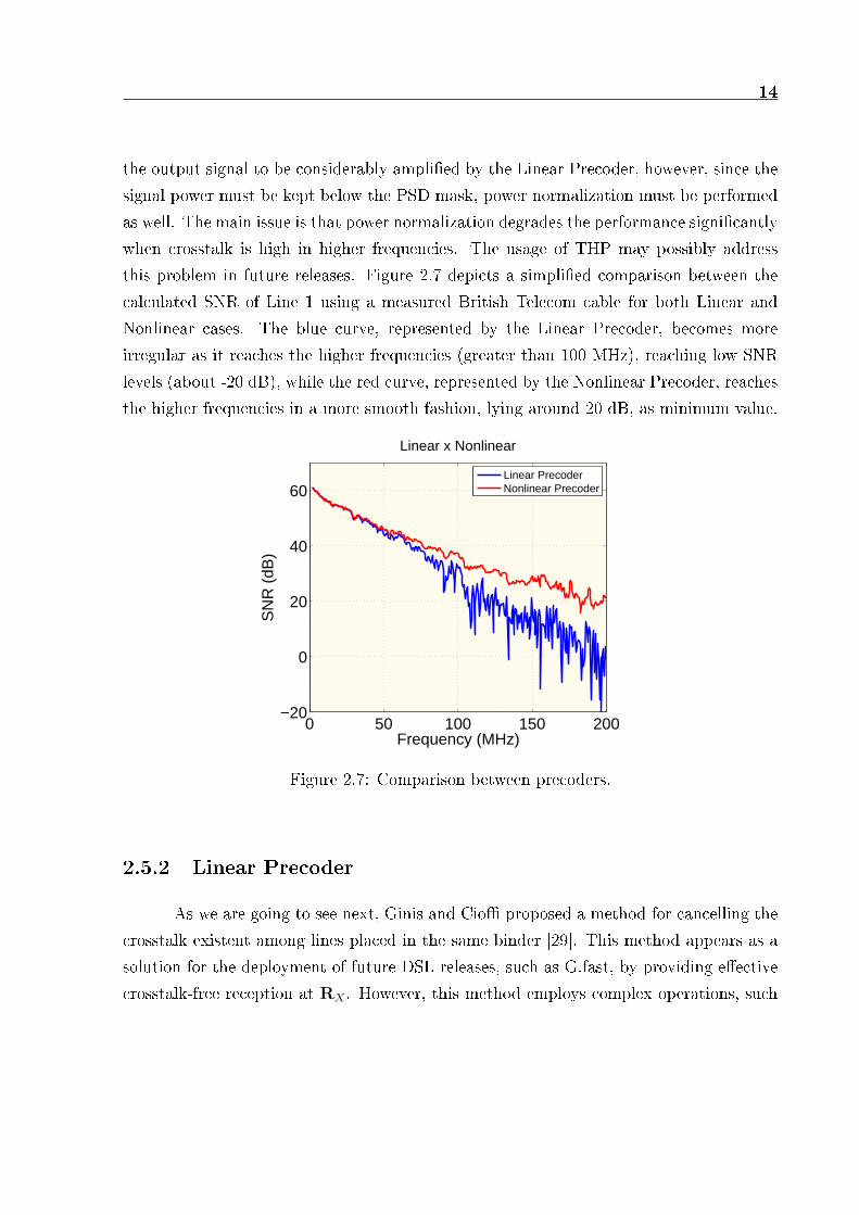
this problem in future releases. Figure 2.7 depicts a simplified comparison between the

calculated SNR of Line 1 using a measured British Telecom cable for both Linear and

Nonlinear cases. The blue curve, represented by the Linear Precoder, becomes more

irregular as it reaches the higher frequencies (greater than 100 MHz), reaching low SNR

levels (about -20 dB), while the red curve, represented by the Nonlinear Precoder, reaches

the higher frequencies in a more smooth fashion, lying around 20 dB, as minimum value.

0 50 100 150 200−20

0

20

40

60

Linear x Nonlinear

Frequency (MHz)

SN

R (

dB)

Linear PrecoderNonlinear Precoder

Figure 2.7: Comparison between precoders.

2.5.2 Linear Precoder

As we are going to see next, Ginis and Cioffi proposed a method for cancelling the

crosstalk existent among lines placed in the same binder [29]. This method appears as a

solution for the deployment of future DSL releases, such as G.fast, by providing effective

crosstalk-free reception at R𝑋 . However, this method employs complex operations, such

15

as the modulo function and requires the CPE structure to be adapted. Hence, it has been

criticized by some authors, such as Cendrillon [27]:

"A decision-feedback structure, based on the Tomlinson-Harashima Precoder

(THP), was shown to operate close to the single-user bound [30]. Unfortunately, this

structure relies on a nonlinear modulo operation at the receiver side, leading to a higher

run-time complexity. For example, in a standard VDSL modem operating at 4000 dis-

crete multitone (DMT) symbols per second, with 4096 tones, the modulo operation would

require an extra 16.3 million instructions per second (MIPS). This will almost double the

complexity of the customer premises (CP) modem, which currently only needs to imple-

ment a frequency-domain equalizer, an operation that also requires 16.3 MIPS. Since CP

modems are now a commodity, cost is an extremely sensitive issue, and any technique

that helps to decrease complexity is extremely beneficial."

And in [31]:

"Existing crosstalk precompensation techniques either give poor performance or

require modification of customer premises equipment (CPE). This is impractical since

there are millions of legacy CPE modems already in use."

With that in mind, Cendrillon presented a near-optimal linear solution for can-

celling crosstalk, which the author named Diagonalizing Precoder (DP), with "much

lower complexity than the THP, since it does not require any additional receiver-side

operations."

The Linear Precoder is demonstrated in the next section.

2.5.2.1 System model

For the employment of the Linear Precoder, it is assumed that all receivers are

co-located (placed in the same area and communicating), perfect channel estimation and

synchronism. Considering that DMT is employed, this allows us to model crosstalk on

each tone – or sub-carrier – independently. So the transmission scheme is represented by

y𝑘 = H𝑘x𝑘 + n𝑘. (2.13)

16

Considering that, in each binder, there are 𝐿 lines, vector x𝑘 represents the trans-

mitted symbols from R𝑋 to T𝑋 and is of the form x𝑘 = [𝑥1𝑘, . . . , 𝑥

𝐿𝑘 ]𝑇 , that is, the trans-

mitted signals from lines 1 . . . 𝐿 on tone 𝑘. Vector y𝑘 has the same structure, however it

represents the received signals. The channel matrix [H𝑘]𝐿×𝐿 contains the complex gains

of the FEXT channel and of the direct channel of each line. The element ℎ𝑖,𝑗𝑘 , [H𝑘]𝑖,𝑗

is the channel from line 𝑗 to line 𝑖 on tone 𝑘, so ℎ𝑘𝑖,𝑗|𝑖 = 𝑗, i.e., the diagonal elements,

represent the direct channels of each line, whereas the non-diagonal elements ℎ𝑘𝑖,𝑗|𝑖 = 𝑗

represent the FEXT channel. The FEXT channel is the crosstalk caused by one line on

the other. This phenomenon is generalized in Figure 2.8.

Figure 2.8: FEXT caused by line 1 on line 2.

Lines ℎ11 and ℎ22 are the direct channels of lines 1 and 2, respectively, and ℎ12 is

the FEXT channel from line 2 to line 1. 𝑇𝐿 and 𝑅𝐿 represent the transmitter and receiver

sides, respectively. The 𝐿× 1 vector n𝑘 contains the additive noise, which is a gathering

of thermal noise, RFI interference, alien crosstalk and so on.

2.5.2.2 The Diagonalizing Precoder

The Linear Precoder is founded on the basic idea of Zero-forcing, the technique

of inverting the channel impulse response, what, in the precoder calculation would mean

simply P = H−1. The problem with this method is the possibility of noise amplifica-

tion [32] [33]. The Diagonalizing Precoder (DP) proposed by Cendrillon makes use of

17

an additional matrix at the transmitter, namely, the diagonal matrix whose diagonal

elements equal those of the channel matrix. This way, the traditional FEQ (Frequency

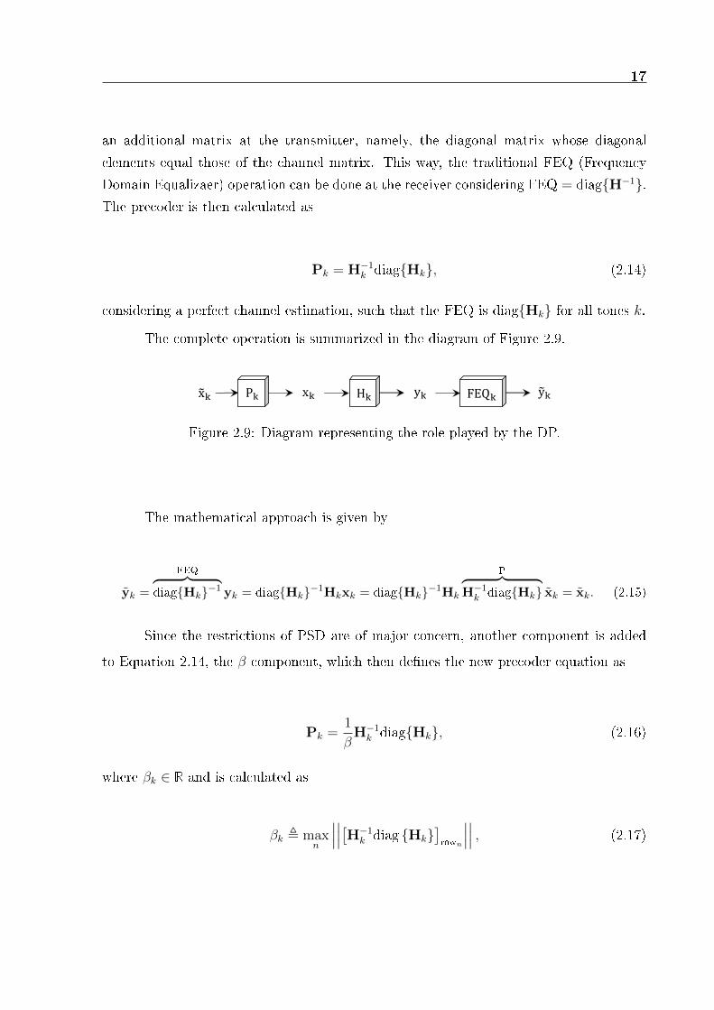
Domain Equalizaer) operation can be done at the receiver considering FEQ = diag{H−1}.The precoder is then calculated as

P𝑘 = H−1𝑘 diag{H𝑘}, (2.14)

considering a perfect channel estimation, such that the FEQ is diag{H𝑘} for all tones 𝑘.

The complete operation is summarized in the diagram of Figure 2.9.

Figure 2.9: Diagram representing the role played by the DP.

The mathematical approach is given by

y𝑘 =

FEQ⏞ ⏟ diag{H𝑘}−1 y𝑘 = diag{H𝑘}−1H𝑘x𝑘 = diag{H𝑘}−1H𝑘

P⏞ ⏟ H−1

𝑘 diag{H𝑘} x𝑘 = x𝑘. (2.15)

Since the restrictions of PSD are of major concern, another component is added

to Equation 2.14, the 𝛽 component, which then defines the new precoder equation as

P𝑘 =1

𝛽H−1

𝑘 diag{H𝑘}, (2.16)

where 𝛽𝑘 ∈ R and is calculated as

𝛽𝑘 , max𝑛

[H−1

𝑘 diag {H𝑘}]row𝑛

, (2.17)

18

which means that 𝛽𝑘 is the maximum row norm among all rows of the resulting matrix

of the product H−1𝑘 diag{H𝑘}. This modification requires the alteration of FEQ as well,

which is now calculated by

FEQ = 𝛽diag{H𝑘}−1. (2.18)

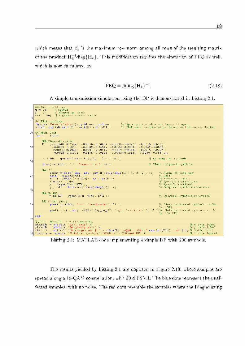
A simple transmission simulation using the DP is demonstrated in Listing 2.1.

%% Basic s e t t i n g sM = 16 ; % M−QAMN = 4; % Number o f u s e r sSNR = 30 ; % Signal−to−no i s e r a t i o

5%% Plot opt ionsf i g u r e ( ’ Color ’ , ’ white ’ ) ; g r id on ; hold on ; % Opens p lo t window and keeps i t openax i s ([− sq r t (M) sq r t (M) −sq r t (M) sq r t (M) ] ) ; % Plot ax i s c on f i gu r a t i on based on the c o n s t e l l a t i o n

10 %% Main Loopf o r L = 1:200

%% Channel matrixH = [−0.0800+0.0582 i −0.0010−0.0003 i −0.0035−0.0020 i −0.0049+0.0017 i ;

15 −0.0032+0.0083 i −0.0602−0.0484 i −0.0054+0.0003 i −0.0147−0.0060 i ;0.0016−0.0036 i −0.0001−0.0011 i −0.0012−0.0661 i −0.0018+0.0082 i ;

−0.0022+0.0109 i −0.0158−0.0019 i −0.0032+0.0018 i 0.0250−0.0667 i ] ;

x_ti lde = qammod( randi ( M, N, 1 ) − 1 , M ) ; % Rx o r i g i n a l symbols20

p lo t ( x_ti lde , ’ . ’ , ’ markers i ze ’ , 25 ) ; % Plots o r i g i n a l symbols

%% DPnorms = sqr t ( sum( abs ( inv (H)*diag ( diag (H) ) ) .^2 , 2 ) ) ; % Norms o f each row

25 beta = max( norms ) ; % BetaP = ( 1/ beta )* inv (H)*diag ( diag (H) ) ; % Precoder matrixx = P*x_ti lde ; % Symbols t ransmittedy = awgn( H*x , SNR ) ; % Symbols r e c e i v edy_ti lde = beta* inv ( diag ( diag (H) ) )*y ; % Or ig ina l symbols recovered

30%% No DP

y_no_DP = awgn( H*x_ti lde , SNR ) ; % Or ig ina l symbols recovered

%% Fina l p l o t s35 p lo t ( y_ti lde , ’ . r ’ , ’ markers i ze ’ , 25 ) ; % Plots recovered symbols at Rx

% (DP)p lo t ( inv ( diag ( diag (H) ) )*y_no_DP, ’ . g ’ , ’ markers i ze ’ , 25 ) ;% Plots recovered symbols at Rx

% (No DP)end

40%% Axis l a b e l i n g and customiz ingxhandle = x l abe l ( ’ Real ax i s ’ ) ; % x ax i s l a b e lyhandle = y l abe l ( ’ Imaginary ax i s ’ ) ; % y ax i s l a b e lthandle = t i t l e ( [ ’DP comparison | ’ num2str (M) ’−QAM | SNR: ’ num2str (SNR) ’ dB ’ ] ) ; % T i t l e l a b e l

45 lhand le = legend ( ’ Or i g ina l symbols ’ , ’With DP’ , ’Without DP’ ) ; % Figure legend

Listing 2.1: MATLAB code implementing a simple DP with 200 symbols.

The results yielded by Listing 2.1 are depicted in Figure 2.10, where samples are

spread along a 16-QAM constellation, with 30 dB SNR. The blue dots represent the unaf-

fected samples, with no noise. The red dots resemble the samples where the Diagnolazing

19

−3 −1 1 3

−3

−1

1

3

Real axis

Imag

inar

y ax

is

DP comparison | 16−QAM | SNR: 30 dB

Original symbolsWith DPWithout DP

Figure 2.10: Comparison between transmissions with and without DP.

Precoder was applied, even with additive noise, and the green dots represent the sam-

ples with additive noise that had no precoding involved. The conclusion is that the DP

was decisive to gather symbols of the same point, whereas the non-precoded symbols are

scattered and with difficult mapping.

2.5.3 The Tomlinson-Harashima Precoder

The Tomlinson-Harashima Precoder, usually abbreviated THP, was the precoding

technique presented, almost simultaneously by Tomlinson and Harashima [25] [26], seeking

at cancelling the crosstalk among lines. Ginis and Cioffi [29] extended this technique to

DSL and complemented the modulo arithmetic.

The Tomlinson-Harashima Precoder is a structure developed for general purposes,

more specifically, an "ISI mitigation structure consisting of a feedback filter in the trans-

20

mitter and a feedforward filter in the receiver." [29] This precoder can be used for in-

terference nulling and interference cancellation, however, it requires joint processing at

the receiver side in point-to-multipoint communication. In the case of DSL, the scenario

where THP could be used is a downlink transmission from the CO for several CPEs. In

this scenario, the main target is the precoding matrix, which is calculated after some

matrix manipulations of the original transmission model.

Suppose we try to transmit M-QAM symbols through a frequency-selective AWGN

fading channel of a discrete-model DSL communication system. The precoding matrix

is calculated for each sub-carrier (tone) 𝑘. The received symbols at R𝑋 are given by

Equation 2.13 and has the same structure (channel matrix, vector of sent and received

symbols and so on).

As already mentioned, the THP utilizes the QR decomposition, a means of decom-

posing one matrix into two others with specific characteristics. So, the channel matrix is

decomposed as

H𝐻𝑘 = Q𝑘R𝑘, (2.19)

where H𝐻𝑘 is the hermitian of matrix H𝑘, i.e., its transpose-conjugate, where the element

in the i -th row and j -th column is equal to the complex conjugate of the element in the

j -th row and i -th column. Decomposing the hermitian of matrix H is a means of yielding

a structure easier to calculate, since it will pretty much rely on matrix R𝑘, as shown in

the sequel. If we expand Equation 2.19, the QR decomposition turns to

H𝑘 = (Q𝑘R𝑘)𝐻 , (2.20)

H𝑘 = R𝐻𝑘 Q

𝐻𝑘 . (2.21)

If we right-multiply (Q𝐻𝑘 )−1 in both sides of Equation 2.21, we obtain

21

H𝑘(Q𝐻𝑘 )−1 = R𝐻

𝑘 . (2.22)

From the definition of unitary matrix [34], it equals its inverse, which in turn equals

its hermitian, so the final relation stands for

H𝑘Q𝑘 = R𝐻𝑘 . (2.23)

Before sending the original symbols from each user through the channel, an inter-

mediate step is required. It is assumed that there is an 𝐿×1 vector x′𝑘 that, left-multiplied

by matrix Q𝑘, yields x𝑘, i.e.,

x𝑘 = Q𝑘x′𝑘. (2.24)

Therefore, placing Equation 2.24 into Equation 2.13, and taking into account Equa-

tion 2.23, we can calculate the symbols received by

y𝑘 = H𝑘Q𝑘x′𝑘, (2.25)

y𝑘 = R𝐻𝑘 x

′𝑘. (2.26)

At the receiver side, vector y𝑘 is left-multiplied by an 𝐿 × 𝐿 diagonal matrix S𝑘,

whose main diagonal equals the main diagonal of matrix R𝑘. This procedure works as the

FEQ, in order to obtain the original symbols from x𝑘, and serves as a means of finding the

relations among the gains of all users. The original x𝑘 symbols equals the final symbols

y𝑘 at R𝑋 , that is,

x𝑘 = y𝑘. (2.27)

22

By including the FEQ matrix S𝑘, we obtain

x𝑘 = S−1𝑘 y𝑘. (2.28)

By left-multiplying S𝑘 in both sides of Equations 2.28 and including Equation 2.26,

we obtain the final transmission relation, which is

S𝑘x𝑘 = y𝑘, (2.29)

S𝑘x𝑘 = R𝐻𝑘 x

′𝑘. (2.30)

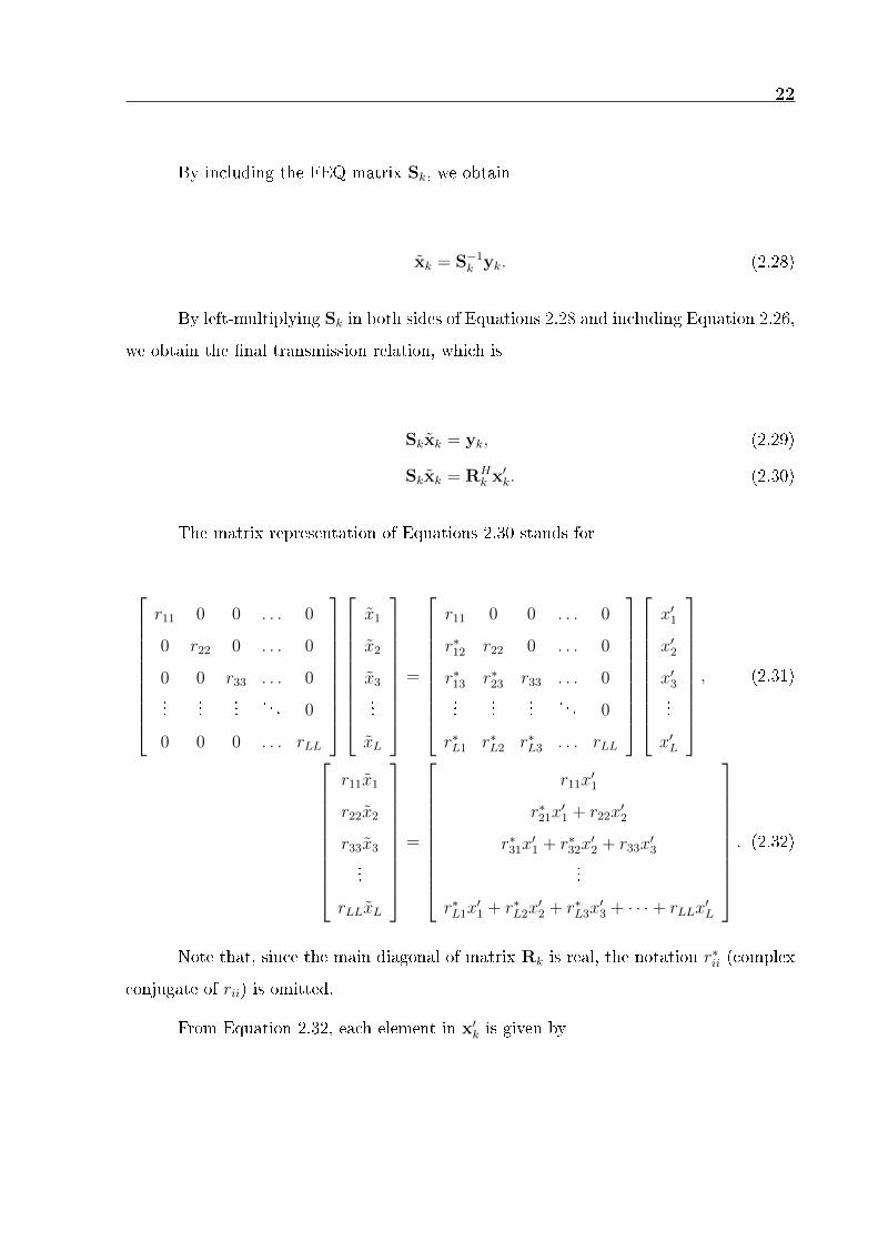
The matrix representation of Equations 2.30 stands for

⎡⎢⎢⎢⎢⎢⎢⎢⎢⎢⎣

𝑟11 0 0 . . . 0

0 𝑟22 0 . . . 0

0 0 𝑟33 . . . 0...

......

. . . 0

0 0 0 . . . 𝑟𝐿𝐿

⎤⎥⎥⎥⎥⎥⎥⎥⎥⎥⎦

⎡⎢⎢⎢⎢⎢⎢⎢⎢⎢⎣

��1

��2

��3

...

��𝐿

⎤⎥⎥⎥⎥⎥⎥⎥⎥⎥⎦=

⎡⎢⎢⎢⎢⎢⎢⎢⎢⎢⎣

𝑟11 0 0 . . . 0

𝑟*12 𝑟22 0 . . . 0

𝑟*13 𝑟*23 𝑟33 . . . 0...

......

. . . 0

𝑟*𝐿1 𝑟*𝐿2 𝑟*𝐿3 . . . 𝑟𝐿𝐿

⎤⎥⎥⎥⎥⎥⎥⎥⎥⎥⎦

⎡⎢⎢⎢⎢⎢⎢⎢⎢⎢⎣

𝑥′1

𝑥′2

𝑥′3

...

𝑥′𝐿

⎤⎥⎥⎥⎥⎥⎥⎥⎥⎥⎦, (2.31)

⎡⎢⎢⎢⎢⎢⎢⎢⎢⎢⎣

𝑟11��1

𝑟22��2

𝑟33��3

...

𝑟𝐿𝐿��𝐿

⎤⎥⎥⎥⎥⎥⎥⎥⎥⎥⎦=

⎡⎢⎢⎢⎢⎢⎢⎢⎢⎢⎣

𝑟11𝑥′1

𝑟*21𝑥′1 + 𝑟22𝑥

′2

𝑟*31𝑥′1 + 𝑟*32𝑥

′2 + 𝑟33𝑥

′3

...

𝑟*𝐿1𝑥′1 + 𝑟*𝐿2𝑥

′2 + 𝑟*𝐿3𝑥

′3 + · · ·+ 𝑟𝐿𝐿𝑥

′𝐿

⎤⎥⎥⎥⎥⎥⎥⎥⎥⎥⎦. (2.32)

Note that, since the main diagonal of matrix R𝑘 is real, the notation 𝑟*𝑖𝑖 (complex

conjugate of 𝑟𝑖𝑖) is omitted.

From Equation 2.32, each element in x′𝑘 is given by

23

x′𝑙 = x𝑙 −

1

𝑟𝑙𝑙

𝑙−1∑𝑗=1

x′𝑗𝑟

*𝑗𝑙. (2.33)

Considering that the symbols to be transmitted are given by x𝑘 = P𝑘x𝑘, and

the received symbols are given by y𝑘 = H𝑘P𝑘x𝑘, the precoding matrix P𝑘 can now be

calculated by

P𝑘 = Q𝑘

[x′𝑘 ∙

1

x𝑘

], (2.34)

where ∙ represents the scalar multiplication between each of x′𝑘 and 1

x𝑘elements. Equa-

tion 2.30 can be reorganized as

S𝑘x𝑘 = R𝐻𝑘 x

′𝑘, (2.35)

x′𝑘 = (R𝐻

𝑘 )−1S𝑘x𝑘. (2.36)

Applying it to Equation 2.34, the precoding matrix P𝑘 is given by

P𝑘 = Q𝑘(R𝐻𝑘 )−1S𝑘x𝑘 ∙

1

x𝑘

, (2.37)

P𝑘 = Q𝑘(R𝐻𝑘 )−1S𝑘. (2.38)

This shows that the precoding operation can be done right after the QR decom-

position step, however, looking at Equation 2.33, one can notice that an energy increase

is likely to happen the bigger the number of subscriber lines. For that matter, the THP

utilizes a handful method to address this issue: the modulo operation.

24

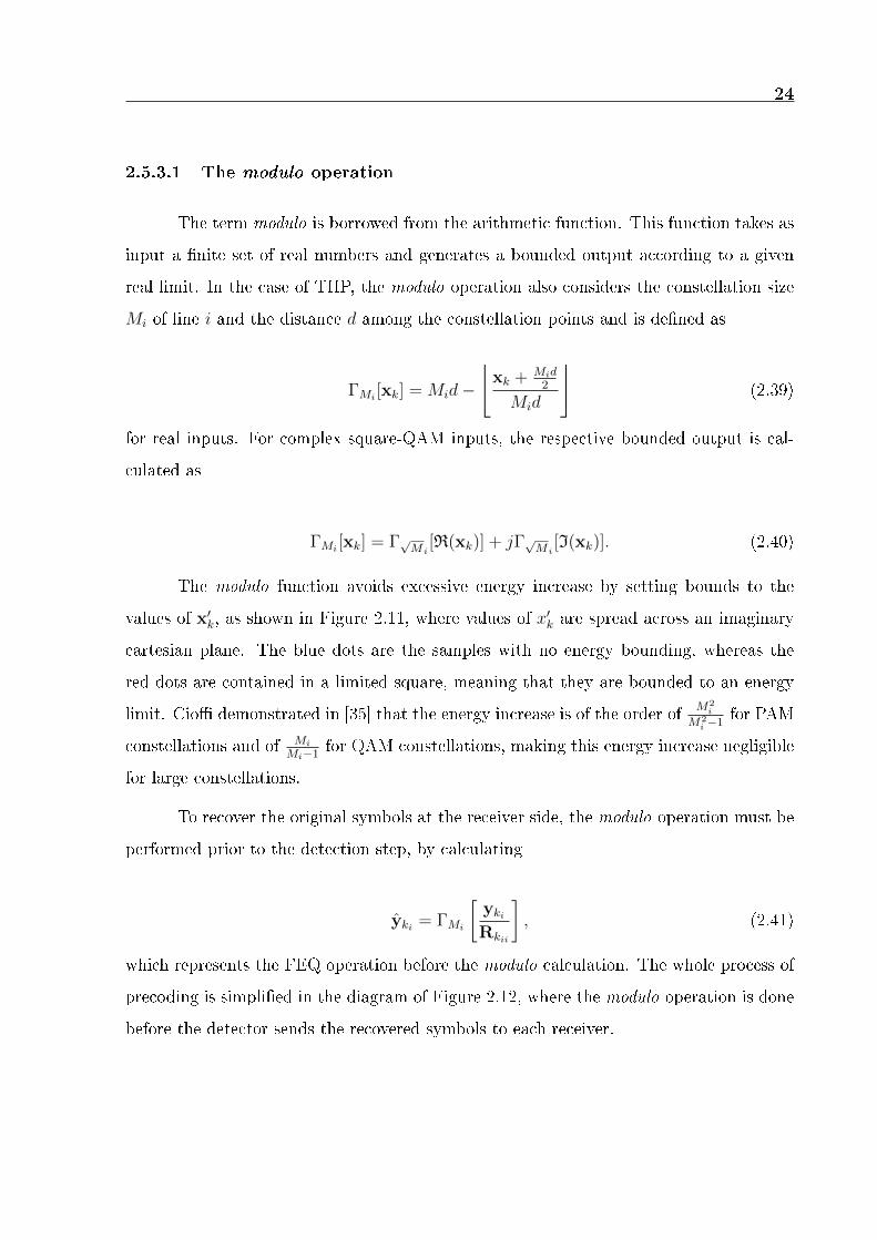
2.5.3.1 The modulo operation

The term modulo is borrowed from the arithmetic function. This function takes as

input a finite set of real numbers and generates a bounded output according to a given

real limit. In the case of THP, the modulo operation also considers the constellation size

𝑀𝑖 of line 𝑖 and the distance 𝑑 among the constellation points and is defined as

Γ𝑀𝑖[x𝑘] = 𝑀𝑖𝑑−

⌊x𝑘 + 𝑀𝑖𝑑

2

𝑀𝑖𝑑

⌋(2.39)

for real inputs. For complex square-QAM inputs, the respective bounded output is cal-

culated as

Γ𝑀𝑖[x𝑘] = Γ√

𝑀 𝑖[R(x𝑘)] + 𝑗Γ√

𝑀 𝑖[I(x𝑘)]. (2.40)

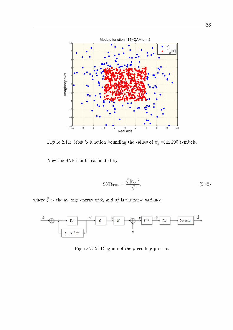
The modulo function avoids excessive energy increase by setting bounds to the

values of x′𝑘, as shown in Figure 2.11, where values of 𝑥′

𝑘 are spread across an imaginary

cartesian plane. The blue dots are the samples with no energy bounding, whereas the

red dots are contained in a limited square, meaning that they are bounded to an energy

limit. Cioffi demonstrated in [35] that the energy increase is of the order of 𝑀2𝑖

𝑀2𝑖 −1

for PAM

constellations and of 𝑀𝑖

𝑀𝑖−1for QAM constellations, making this energy increase negligible

for large constellations.

To recover the original symbols at the receiver side, the modulo operation must be

performed prior to the detection step, by calculating

y𝑘𝑖 = Γ𝑀𝑖

[y𝑘𝑖

R𝑘𝑖𝑖

], (2.41)

which represents the FEQ operation before the modulo calculation. The whole process of

precoding is simplified in the diagram of Figure 2.12, where the modulo operation is done

before the detector sends the recovered symbols to each receiver.

25

−10 −8 −6 −4 −2 0 2 4 6 8 10−10

−8

−6

−4

−2

0

2

4

6

8

10Modulo function | 16−QAM d = 2

Real axis

Imag

inar

y ax

is

x’Γ

16[x’]

Figure 2.11: Modulo function bounding the values of x′𝑘 with 200 symbols.

Now the SNR can be calculated by

SNRTHP =𝜉𝑖|𝑟𝑖,𝑖|2

𝜎2𝑖

, (2.42)

where 𝜉𝑖 is the average energy of x𝑖 and 𝜎2𝑖 is the noise variance.

Figure 2.12: Diagram of the precoding process.

26

Listing 2.2 simulates a transmission system with 4 lines applying the above-

mentioned precoding techniques.

c l c%% Basic v a r i a b l e sL = 4 ; % Number o f u s e r sM = 16 ; % Cons t e l l a t i on s i z e

5 d = 2 ; % Distance between po int sSNR = 30 ; % Signal−to−no i s e r a t i o

%% Transmiss ion va r i a b l e sx_ti lde = qammod( randi (M,L , 1 )−1,M) ; % Randomly generated QAM symbols

10H = [ −0.0093+0.0123 i 0.0001+0.0035 i 0.0007+0.0035 i 0.0043−0.0031 i ;

−0.0008+0.0011 i 0.0011−0.0127 i −0.0024−0.0014 i 0.0008+0.0034 i ;0.0004−0.0016 i 0.0010−0.0004 i 0.0025−0.0008 i 0.0018−0.0016 i ;

−0.0021−0.0019 i 0.0005+0.0002 i −0.0016−0.0018 i 0.0010+0.0011 i ; ] ;15

% LxL channel matrix

%% Main t ransmi s s i on without modulo[Q,R] = qr (H’ ) ; % QR decomposit ion o f

20 % the hermit ian o f H (Eq . 2 . 19 )

S = diag ( diag (R) ) ; % LxL FEQ matrix .% I t s main d iagona l equa l s the main d iagona l% of matrix R

25 P = Q*(R’ ) ^−1*S ; % Precodery = awgn(H*P*x_ti lde , SNR, ’ measured ’ ) ; % Al l symbols are

% sent through the channely_ti lde = S^−1*y ; % The o r i g i n a l symbols

% are recovered a f t e r the FEQ operat ion30

%% Main t ransmi s s i on with modulo[Q,R] = qr (H’ ) ; % QR decomposit ion o f

% the hermit ian o f H (Eq . 2 . 19 )x_prime = ze ro s ( s i z e ( x_ti lde ) ) ; % Al l o ca t e s memory f o r x ’

35 f o r i = 1 :L % Loop f o r c a l c u l a t i n g x ’x_prime ( i ) = x_ti lde ( i ) ; % Eq . 2 .33f o r j = 1 : i−1x_prime ( i ) = x_prime ( i ) − (1/R( i , i ) )*x_prime ( j )* conj (R( j , i ) ) ;end

40 end

x_prime_m = cc_modulo (M, d , x_prime ) ; % Eq . 2 .39x = Q*x_prime_m ; % Eq . 2 .24y = awgn(H*x , SNR) ; % Channel t ransmi s s i on

45 y_ti lde = S^−1*y ; % FEQ at r e c e i v e rf o r i = 1 :L

x_tilde_hat ( i ) = cc_modulo (M, d , y_ti lde ( i ) . /R( i , i ) ) ; % Eq . 2 .41end

Listing 2.2: MATLAB listing that simulates the THP in DSL transmission systems.

Chapter 3

RATE-BALANCING TECHNIQUES

As already addressed in this work, rate-balancing attempts to diminish the bitrate

difference among lines, consequence of the Nonlinear Precoder, since an essencial charac-

teristic of its structure may affect some lines to the detriment of others: the Gram-Schmidt

decomposition, in which the QR decomposition is based.

As seen in Chapter 2, Gram-Schmidt decomposition arbitrarily takes the first col-

umn of the channel matrix as the starting vector for calculating the projections and the

remaining u vectors. In other words, the first user, here represented by the first column,

has no gain loss (caused by the QR decomposition), as stated by the GS formula, whereas

the following columns are always subtracted from the projections of the previous columns.

Figure 3.1 shows this phenomenon graphically, as the bitrate values slightly decrease when

reaching the last lines in two Swisscom cables. One can notice that the difference between

the last lines (from 1 to 10 or 20) and the first lines is considerable. For example, in the

P-ALT cable, the last line represents only 54.61% of the bitrate from the first line.

In QR decomposition, an orthogonal basis {e1, e2, . . . , e𝑁} is formed in the channel

vector space H𝐻 , where e𝑖 is the 𝑖-th orthogonal base vector. As shown in Equation 2.42,

the effective channel gain of the 𝑖-th line in the line order, 𝑟𝑖𝑖, is the projection from

27

28

the channel vector of the line to the corresponding 𝑖-th orthogonal base vector. The

orthogonal basis depends on how the lines are ordered in QR decomposition. Therefore,

the effective channel gain, i.e., the projection, also varies. It was demonstrated in [36] that

varying the ordering in THP can cause up to 75% increase from minimum to maximum

bitrate of a 100 m loop.

1 4 7 101650

1700

1750

1800

1850

1900

1950

2000

2050Swisscom I51

Line

Rat

es (

Mbp

s)

Tomlinson−Harashima

1 5 10 15 20700

800

900

1000

1100

1200

1300Swisscom P−ALT

Line

Rat

es (

Mbp

s)

Tomlinson−Harashima

Figure 3.1: Penalization of last lines.

That being said, the main task now is to find the best column sorting of the channel

matrix H, changing the way each line affects the other after the QR decomposition. This

technique is performed at each tone 𝑘 and is simplified in Figure 3.2.

Figure 3.2: Column sorting for achieving rate-balancing.

Each balancing method has its own metrics to define how the channel will be

reorganized. The idea behind this procedure is that the transmitter at downstream,

29

has total knowledge of each line, since the channel was previously estimated. So the

precoding operation changes only the ordering of columns, meaning that when the actual

transmission occurs, each receiver will get exactly the data it was meant to receive. This

complexity is added at the transmitter and only minor changes at the receiver are needed,

as already explained in section 2.5.3.

3.1 GS-SORTING

The GS-Sorting method consists of a simple, yet expensive, procedure of doing

iterative Gram-Schmidt decompositions on every submatrix formed by the original ma-

trix H𝑘 of a given tone 𝑘, starting from its first column to the last one. The principle

is to consider each column as a vector for the GS-decomposition to subtract the projec-

tions of other columns (lines) over themselves. The complete procedure is explained in

Algorithm 1.

Algorithm 1 GS-Sorting

1: function GS-Sorting(H𝑘) ◁ 𝐻𝑘 is the matrix of a given tone k

2: L: Number of lines ◁ Definition of variables

3: H′𝑘 ← H𝐻

𝑘

4: for 𝑖 = 1→ 𝐿 do

5: normH′𝑘(𝑖)← ‖col𝑖{H′

𝑘}‖

6: indices← sort(normH′𝑘,’ascending ’) ◁ Original indices of ascending sorting

7: 𝑖← 2

8: while 𝑖 <= L do

9: H𝑘 ← cols(H′𝑘, 𝑖→ L) ◁ 𝐻𝑘 is a submatrix from column 𝑖 to L

10: H𝑘 ← gs(H𝑘) ◁ Regular G.Schmidt decomposition

11: minNormCol ←minCol(H𝑘) ◁ Index of the least norm column

30

12: H𝑘 ← swapCols(H𝑘, 1,minNormCol) ◁ Swap cols 1 and minNormCol of H𝑘

13: indices(𝑖)←indices(minNormCol + 𝑖− 1)

14: cols(H′𝑘, 𝑖→ 𝐿)← H𝑘 ◁ Update H′

𝑘 in columns 𝑖 to L

15: 𝑖← 𝑖 + 1

16: return H′𝑘

3.2 POST-SORTING

The next rate-balancing method proposed by this work is the so-called Post-sorting

method. It is named this way due to its simple functionality of comparing the direct

channel of each line prior to QR decomposition with norms of the columns of matrix R.

The algorithm then sorts the lines based on their respective before-after ratios, where the

first columns of the sorted matrix contain the lines with the smaller ratios and the last

columns contain the larger ones. The idea behind this method is that lines with small

before-after ratios have weak direct channels compared to their norms in matrix R, whose

diagonal values consider FEXT as well. These lines must then be positioned somewhere

in the channel matrix where they will not be penalized by the QR decomposition. On

the other hand, lines with big ratios have stronger direct channels and will probably not

lose much after QR decomposition. Since the QR decomposition must be done at least

twice, this method might take longer to process. Comparative numbers will be presented

in Chapter 4. The Post-sorting method is detailed in Algorithm 2.

Algorithm 2 Post-Sorting Algorithm

1: L: Number of lines ◁ Definition of variables

2: function PS(H𝑘)

3: [Q𝑘,R𝑘]← qr(H𝐻𝑘 ) ◁ Regular QR decomposition

4: for 𝑖 = 1→ L do

5: normR𝑘(𝑖)← ‖col𝑖{R𝑘}‖

31

6: ratios ← ‖diag{H𝑘}‖normR𝑘

◁ Ratio between (Direct-channel/After-QR)

7: indices ← sort(ratios,’ascending ’) ◁ Stores indices order according to ratios

8: H′𝑘 ← sort(H𝐻

𝑘 , indices)

9: return H′𝑘 ◁ Returns sorted matrix

3.3 ORIGINAL SORTING

The Original sorting is a method that involves a simple sort of the channel matrix

for each worked tone 𝑘. This simple sort rearranges the channel matrix based solely on

the norm of each column, iteratively moving the columns with greater norm values to

the last positions (rightwards). The norm-reordering method presents, as positive aspect,

the low complexity, hence, the low computational cost. This method follows the same

methodology from the Post-sorting, with the simple difference that the sorting parameter

is solely the norm of columns. This method is briefly listed in Algorithm 3, where H𝑘 is

the channel matrix for the given tone 𝑘 and the parameter ’ascending’ means the matrix

is reordered in a smaller-bigger fashion.

Algorithm 3 Original-Sorting Algorithm

1: function OS(H𝑘)

2: L: Number of lines ◁ Definition of variables

3: H′𝑘 ← H𝐻

𝑘 ◁ Calculates the hermitian of the channel matrix

4: for 𝑖 = 1→ L do

5: normsH′𝑘← ‖col𝑖{H′

𝑘}‖ ◁ Norms of each column

6: indices ← sort(normsH′𝑘,’ascending ’) ◁ Gets the indices order according to norm

values

7: H′′𝑘 ← sort(H′

𝑘, indices)

8: return H′′𝑘 ◁ Returns the sorted channel matrix

32

3.4 GENETIC ALGORITHM SORTING

When putting together computer simulations and data with big sample spaces,

finding the optimal solution might be an exhaustive task, if not unaccomplishable. Since

the above-mentioned balancing methods do not guarantee perfect performance, tools such

as the Genetic Algorithm may help achieving these goals, at least for comparison purposes

and for determining the bounds of rate-balancing.

3.4.1 Structure

Since all methods try to find the best column sorting, a proper way to testify their

efficiency would be to compare their results to the optimal solution, that is, the ideal case

where each line gets the same data rate. The best solution turns to be the best possible

column sorting that yields the least varying data rates. That being said, each individual

in the GA simulation is structured as shown in Figure 3.3, where each gene 𝑔 contains

the line index that will be sorted in the corresponding position 𝑔 at the channel matrix.

17 2 9 5 3 6 10 8 4

Chromosome

Figure 3.3: Chromosome’s structure for a 10-line cable.

The number of genes 𝐿 matches the number of lines of the considered cable.

33

3.4.2 Crossover

The crossover operation is performed by selecting two Parent chromosomes with

the roulette wheel method, and then crossed at a rate of 100% at the crossover point

⌊𝐿2⌋, where 𝐿 is the total number of lines. Figure 3.4 depicts the reproduction of two

chromosomes of a 10-line cable, yielding a child, consisting of the genetic information of

its parents.

17 2 9 5 3 6 10 8 4

75 1 2 9 8 4 3 6 10

Parent 1

Parent 2

17 2 9 5 8 4 3 6 10

Child

Figure 3.4: Crossover of two parent chromosomes.

The generated offspring may or may not suffer from Mutation, that is, a random

gene is swapped with another, under a probability of 20%, thus guaranteeing genetic

diversity. Figure 3.5 shows this process in detail.

17 2 9 5 8 4 3 6 10

67 2 9 5 8 4 3 1 10

Figure 3.5: Illustration of the Mutation process.

When all crossovers are done for a given generation, the individual with the best

fitness value is automatically passed to the next generation, characterizing the Elitism

process. That guarantees the best individual will be in the next generation.

34

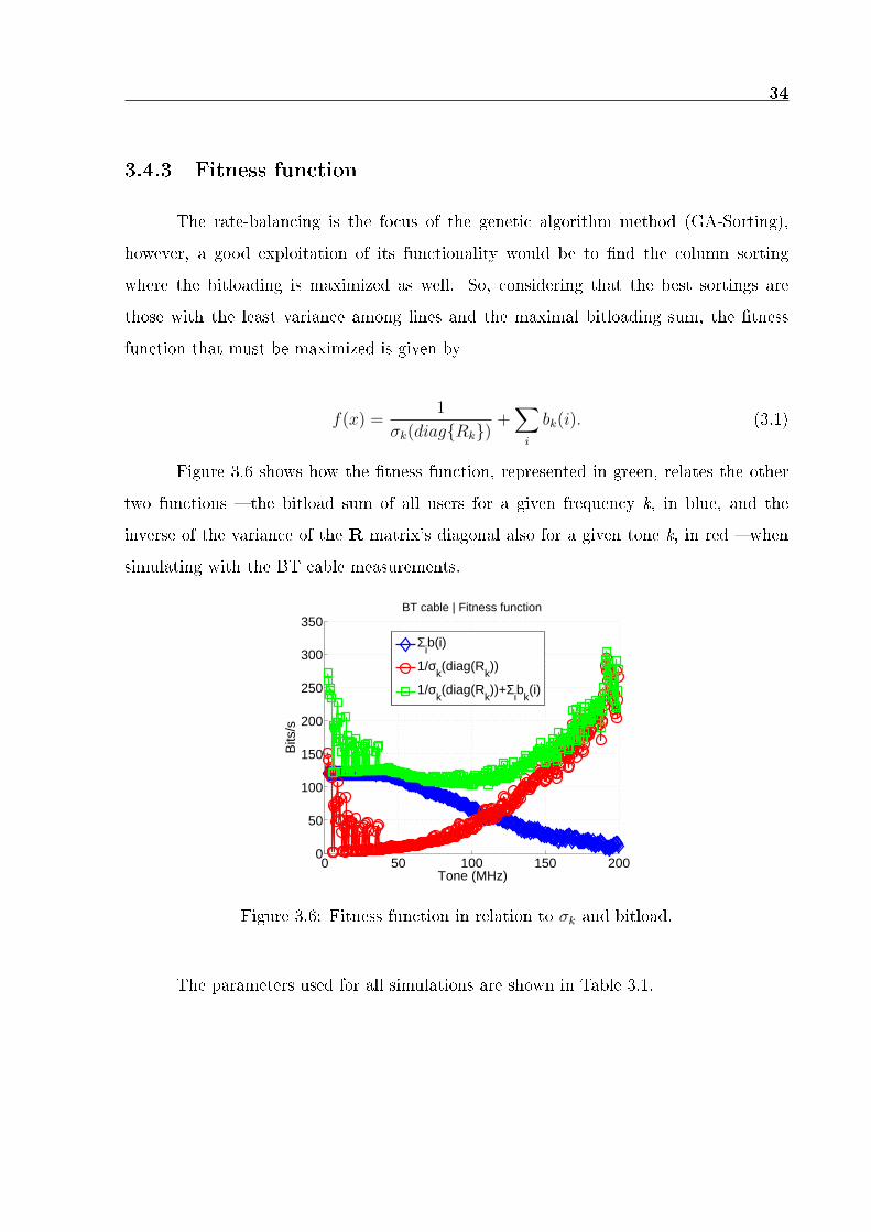
3.4.3 Fitness function

The rate-balancing is the focus of the genetic algorithm method (GA-Sorting),

however, a good exploitation of its functionality would be to find the column sorting

where the bitloading is maximized as well. So, considering that the best sortings are

those with the least variance among lines and the maximal bitloading sum, the fitness

function that must be maximized is given by

𝑓(𝑥) =1

𝜎𝑘(𝑑𝑖𝑎𝑔{𝑅𝑘})+∑𝑖

𝑏𝑘(𝑖). (3.1)

Figure 3.6 shows how the fitness function, represented in green, relates the other

two functions – the bitload sum of all users for a given frequency k, in blue, and the

inverse of the variance of the R matrix’s diagonal also for a given tone k, in red – when

simulating with the BT cable measurements.

0 50 100 150 2000

50

100

150

200

250

300

350

Tone (MHz)

Bits

/s

BT cable | Fitness function

Σib(i)

1/σk(diag(R

k))

1/σk(diag(R

k))+Σ

ib

k(i)

Figure 3.6: Fitness function in relation to 𝜎𝑘 and bitload.

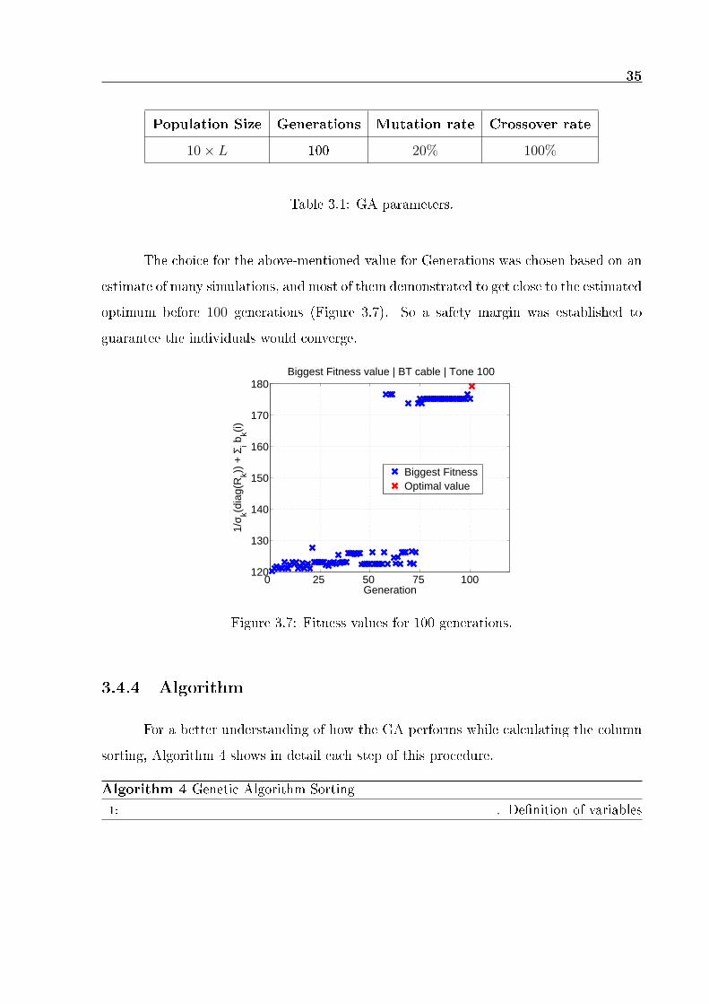
The parameters used for all simulations are shown in Table 3.1.

35

Population Size Generations Mutation rate Crossover rate

10× 𝐿 100 20% 100%

Table 3.1: GA parameters.

The choice for the above-mentioned value for Generations was chosen based on an

estimate of many simulations, and most of them demonstrated to get close to the estimated

optimum before 100 generations (Figure 3.7). So a safety margin was established to

guarantee the individuals would converge.

0 25 50 75 100120

130

140

150

160

170

180

Generation

1/σ k(d

iag(

Rk))

+ Σ

i bk(i)

Biggest Fitness value | BT cable | Tone 100

Biggest FitnessOptimal value

Figure 3.7: Fitness values for 100 generations.

3.4.4 Algorithm

For a better understanding of how the GA performs while calculating the column

sorting, Algorithm 4 shows in detail each step of this procedure.

Algorithm 4 Genetic Algorithm Sorting

1: ◁ Definition of variables

36

2: G: Generations, P: Population, AF: Absolute-Fitness, RF: Relative-Fitness, NP: New

Population

3: function GA-Sorting(H𝑘)

4: P← Random_permutation() ◁ Initial population

5: for 𝑔 = 1→ G do

6: AF ← fitness(P) ◁ Fitness of all Population

7: RF ← AF∑𝑖 AF(𝑖)

◁ Relative fitness of each individual

8: [RF,indices] ← sort(RF,′ascending′) ◁ Sorts RF in an ascending way

9: for 𝑖 = 2→ size(P) do ◁ Organizes the roulette from 0 to 1

10: RF(𝑖) ← RF(𝑖) + RF(𝑖− 1)

11: NP(1) ← P(indices(𝑒𝑛𝑑)) ◁ Elitism

12: for 𝑝 = 2→ size(P) do ◁ Reproduction

13: while Child𝑝 has no duplicate entries do

14: Parent1 ← P(rand())

15: Parent2 ← P(rand())

16: Child𝑝 ← crossover(Parent1, Parent2)

17: NP(𝑝) ← mutation(Child𝑝, mutRate)

18: AF ← fitness(NP) ◁ Fitness of the last Population

19: [AF,indices] ← sort(AF,′ascending′)

20: bestChromosome ← NP(indices(𝑒𝑛𝑑)) ◁ The best individual

21: ◁ of the last Population

22: return bestChromosome

Chapter 4

RESEARCH RESULTS

This chapter presents the results achieved by simulating using measured cables in

the MATLAB environment. For the sake of clarity, below are listed important points that

dictate how the simulations were made, which cables were used and so on.

4.1 SIMULATED CABLES

In order to achieve a good approximation of the benefits provided by the rate-

balancing methods, the simulations should at best consider several cables, since it is an

adequate way of visualizing how these methods behavior in different scenarios – what

should eventually determine their efficiency in the real world networks. Simulations were

held using available measured cables from different manufacturers. Most cable files are

released for a select audience for research purposes, mostly ITU-T associates [37].

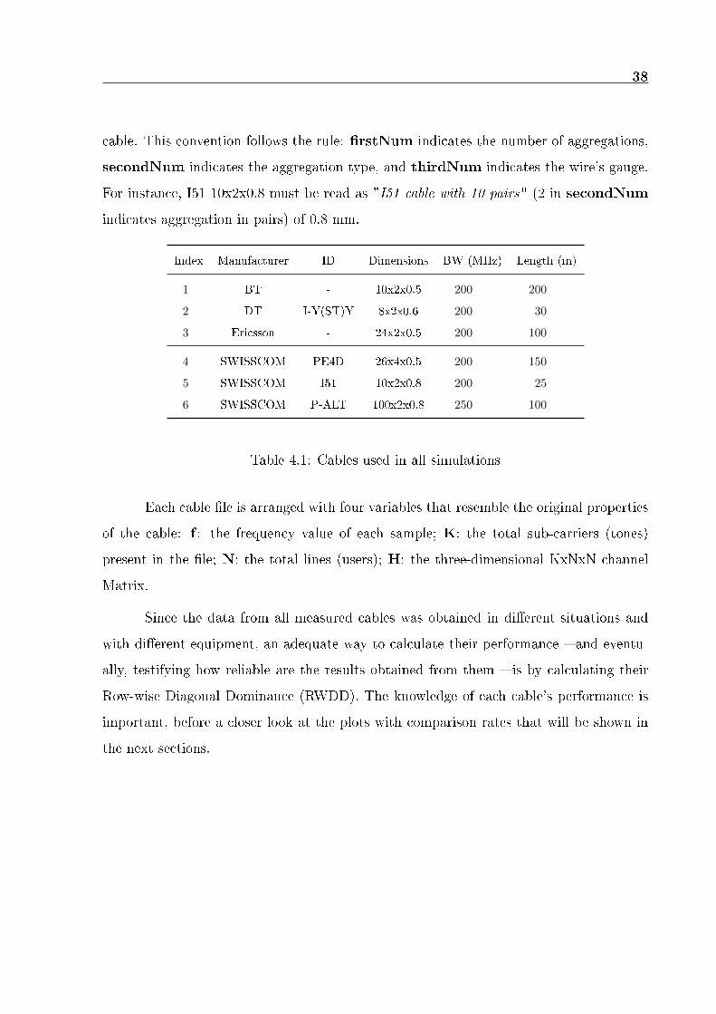
Table 4.1 enumerates the cable files used in all scenarios of simulations and

specifies some characteristics such as bandwidth and length. Column ID shows

the cable types, column Dimensions specifies their characteristics with the syntax

"firstNumxsecondNumxthirdNum", i.e., the way the wires are organized inside the

37

38

cable. This convention follows the rule: firstNum indicates the number of aggregations,

secondNum indicates the aggregation type, and thirdNum indicates the wire’s gauge.

For instance, I51 10x2x0.8 must be read as "I51 cable with 10 pairs" (2 in secondNum

indicates aggregation in pairs) of 0.8 mm.

Index Manufacturer ID Dimensions BW (MHz) Length (m)

1 BT - 10x2x0.5 200 200

2 DT I-Y(ST)Y 8x2x0.6 200 30

3 Ericsson - 24x2x0.5 200 100

4 SWISSCOM PE4D 26x4x0.5 200 150

5 SWISSCOM I51 10x2x0.8 200 25

6 SWISSCOM P-ALT 100x2x0.8 250 100

Table 4.1: Cables used in all simulations

Each cable file is arranged with four variables that resemble the original properties

of the cable: f : the frequency value of each sample; K: the total sub-carriers (tones)

present in the file; N: the total lines (users); H: the three-dimensional KxNxN channel

Matrix.

Since the data from all measured cables was obtained in different situations and

with different equipment, an adequate way to calculate their performance – and eventu-

ally, testifying how reliable are the results obtained from them – is by calculating their

Row-wise Diagonal Dominance (RWDD). The knowledge of each cable’s performance is

important, before a closer look at the plots with comparison rates that will be shown in

the next sections.

39

4.1.1 Row-wise Diagonal Dominance

Before comparing rates among the cables presented in Table 4.1, an adequate

way to check the performance of each one is to look at the Row-wise Diagonal Domi-

nance. It has been noted that xDSL channel matrices are column-wise diagonally domi-

nant (CWDD), while downstream matrices are RWDD. This diagonal-dominance channel

matrix structure is one of the main features that distinguish DSL systems from other

MIMO systems [38]. The RWDD measure (in the literature it is represented as 𝛽 [27],

but it will be switched to 𝛿 to avoid conflicts with the Linear Precoder’s unity) is calculated

as

𝛿row = max𝑖

∑𝑗 =𝑖 |ℎ𝑘

𝑖,𝑗||ℎ𝑘

𝑖,𝑖|, (4.1)

where ℎ𝑘𝑖,𝑗 is the element of matrix H𝑘 in the 𝑖-th row and 𝑗-th column.

A matrix that satisfies 𝛿row < 1 is said to be strongly RWDD, meaning that the

direct channel of every line in matrix H𝑘 is bigger than the sum of all crosstalk it receives.

Equation (2) in [27] states another measure: the ratio between the largest crosstalk value

and the direct channel for that specific sub-channel 𝑘 for each row (𝛼𝑘), and is given by

𝛼𝑘 = max𝑖

max𝑗 =𝑖 |ℎ𝑘𝑖,𝑗|

|ℎ𝑘𝑖,𝑖|

. (4.2)

Figure 4.1 shows the results of each one of the six measured cables when calculating

Equation 4.2, for a better overview of how strong the crosstalk is in comparison to the

direct channel gains.

Some cables showed a steadier RWDD curve as the frequency increases, such as

DT and Ericsson. Actually, the RWDD did not cross the zero line for these two cables,

meaning the direct channel was bigger than the largest crosstalk value at all tones. On

40

the other hand, Swisscom cables P-ALT and PE4D crossed this line before 100 MHz and

got more variant curves. The impact of RWDD is shown in Section 4.1.4.

0 40 80 120 160 200

−20

0

20

40

60

Frequency (MHz)

Dia

gona

l dom

inan

ce (

dB)

RWDD | All worked cables

BTDTEricssonSwiss I51Swiss P−ALTSwiss PE4D

Figure 4.1: Row-wise Diagonal Dominance for each worked cable.

4.1.2 Near-Far scenario

In order to better explore the benefits provided by the proposed methods, the

simulations were extended to the Near-Far scenario. This scenario represents the situation

where lines have different cable length, what should directly affect the data rate they will

get at the CPE and the FEXT they will cause to or receive from other users. However,

it is important to emphasize that this method has not yet been validated, and currently

there is no support for this methodology in platforms such as FTW, in the 100-200 MHz

scenario. That being said, the Near-Far scenario will be used just as a reference.

Since all cable measurements present in Table 4.1 are of Equal-length, a heuristic

was applied in order to obtain the channel files that could represent them. For each cable

file, all lines were split into two groups. The first group, of⌊𝐿2

⌋lines, represents the lines

that resemble lines with longer lengths. The other group remains Equal-length. For the

first group, the direct channel is calculated as

41

H𝑘𝑁𝐹(𝑚,𝑚) = H𝑘(𝑚,𝑚)2, (4.3)

where 𝑚 = 1, . . . , ⌊𝐿2⌋. The assumption is that all direct channel values of the extended

pairs are attenuated at an approximate rate (their own squared values). On the other

hand, the FEXT channel considers the direct channel of the interfering line, by multiplying

its value by the original FEXT channel, that is, ∀𝑚 = 𝑛,

H𝑘𝑁𝐹(𝑚,𝑛) = H𝑘(𝑚,𝑛)×H𝑘(𝑛, 𝑛), (4.4)

where 𝑚 = ⌊𝐿2⌋+ 1, . . . , 𝐿 and 𝑛 = 1, . . . , ⌊𝐿

2⌋.

Figure 4.2 demonstrates how the Near-Far scenario is represented, where red arrows

resemble the FEXT channel.

Figure 4.2: Representation of the Near-Far scenario with 4 lines.

4.1.3 Comparison rates

The plots shown in the next section depict how the rate-balancing methods – Post-

sorting (PS), Gram-Schmidt (GS) and Original Sorting (OS) – behaved in comparison

to the traditional Tomlinson-Harashima Precoder (THP) and the Single-line (SL) case,

i.e., the direct channel of all users, not considering the FEXT caused by other lines.

The comparison was extended to the above-mentioned Near-Far scenario for an extended

analysis, so both cases are depicted together for each cable. Likewise, tables for each cable

42

bring data about total rate sum, the standard deviation and the minimum and maximum

rates for each method, in both Equal-length and Near-Far scenarios. Also present in the

table are the average processing time for each method, considering milliseconds per tone

(ET). All these quantities are shown in Gbps, except for standard deviation. Since its

representation in Gbps would not suggest big differences, it will be shown in Mbps.

4.1.3.1 BT cable

When simulating with BT cables, as displayed in Figures 4.3a and 4.3b, most

rate-balancing methods behaved similarly to each other, in both the Equal-length and

Near-Far scenarios, considering the Standard deviation.

1 2 3 4 5 6 7 8 9 10900

1000

1100

1200

1300

1400

1500BT cable | Rates

Line

Rat

es (

Mbp

s)

THPSLPSGSOSGA

(a) Equal-length

1 2 3 4 5 6 7 8 9 10200

400

600

800

1000

1200

1400BT cable | Rates

Line

Rat

es (

Mbp

s)

THPSLPSGSOSGA

(b) Near-Far

Figure 4.3: British Telecom cable rates.

They could achieve a balancing rate sufficient for approximating all lines, at least

regarding the graphical view. The real performance difference can be verified when looking

at the numbers of each case in Table 4.2, with a special look to standard deviation and

the elapsed time of processing.

In the Equal-length case, not considering the GA method, that reached the least

43

Std value (6.92), the Original sorting method has a slight advantage in comparison to

others, so it is reasonable to say that it achieved the best balancing among lines, whereas

in the Near-Far scenario, the Post-sorting method performed better, however taking ap-

proximately 0.02 ms more for calculating an individual tone.

Equal length Near-Far

SL THP PS GS OS GA SL THP PS GS OS GA

Sum (Gbps) 11.51 11.94 11.91 11.87 11.92 11.98 8.06 9.69 9.66 9.41 9.47 9.73

Std (Mbps) 138.42 131.47 14.18 9.82 9.42 6.92 392.74 92.88 41.92 63.07 63.39 14.17

Max (Gbps) 1.32 1.42 1.21 1.21 1.20 1.21 1.28 1.13 1.04 1.01 1.03 0.99

Min (Gbps) 0.98 1.03 1.16 1.17 1.17 1.18 0.38 0.83 0.92 0.87 0.87 0.95

ET (ms) 0.11 0.35 0.21 7.78 0.19 2209.71 0.11 0.35 0.21 7.91 0.19 2217.27

Table 4.2: BT cable rates.

4.1.3.2 DT cable

On the other hand, with a closer look to plots in Figures 4.4a and 4.4b, that

represent the results obtained for the DT I-Y(ST)Y cable, one can notice that the rate-

balancing methods performed considerably better for the Equal-length case in comparison

to the Near-Far case.

Equal length Near-Far

SL THP PS GS OS GA SL THP PS GS OS GA

Sum (Gbps) 15.77 15.83 15.83 15.83 15.83 15.83 12.73 13.60 13.60 13.60 13.60 13.58

Std (Mbps) 11.75 10.51 4.80 2.37 2.63 2.52 400.64 214.95 213.87 209.80 209.47 43.70

Max (Gbps) 2.00 2.00 1.98 1.98 1.98 1.98 1.97 1.91 1.92 1.92 1.92 1.75

Min (Gbps) 1.96 1.97 1.97 1.97 1.97 1.98 1.19 1.40 1.44 1.49 1.49 1.64

ET (ms) 0.11 0.23 0.20 4.25 0.19 1756.17 0.10 0.24 0.19 4.01 0.18 1639.96

Table 4.3: DT I-Y(ST)Y cable rates.

This fact is observed when comparing the standard deviation values of the rate-

balancing methods with the THP result, where the least Std value of the Equal-length

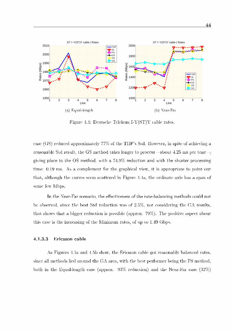
44

1 2 3 4 5 6 7 81950

1960

1970

1980

1990

2000

2010DT I−Y(ST)Y cable | Rates

Line

Rat

es (

Mbp

s)

THPSLPSGSOSGA

(a) Equal-length

1 2 3 4 5 6 7 81000

1200

1400

1600

1800

2000DT I−Y(ST)Y cable | Rates

Line

Rat

es (

Mbp

s)

THPSLPSGSOSGA

(b) Near-Far

Figure 4.4: Deutsche Telekom I-Y(ST)Y cable rates.

case (GS) reduced approximately 77% of the THP’s Std. However, in spite of achieving a

reasonable Std result, the GS method takes longer to process – about 4.25 ms per tone –,

giving place to the OS method, with a 74.9% reduction and with the shorter processing

time: 0.19 ms. As a complement for the graphical view, it is appropriate to point out

that, although the curves seem scattered in Figure 4.4a, the ordinate axis has a span of

some few Mbps.

In the Near-Far scenario, the effectiveness of the rate-balancing methods could not

be observed, since the best Std reduction was of 2.5%, not considering the GA results,

that shows that a bigger reduction is possible (approx. 79%). The positive aspect about

this case is the increasing of the Minimum rates, of up to 1.49 Gbps.

4.1.3.3 Ericsson cable

As Figures 4.5a and 4.5b show, the Ericsson cable got reasonably balanced rates,

since all methods lied around the GA area, with the best performer being the PS method,

both in the Equal-length case (approx. 93% reduction) and the Near-Far case (32%)

45

according to Table 4.4.

1 5 10 15 20 251700

1750

1800

1850

1900Ericsson cable | Rates

Line

Rat

es (

Mbp

s)

THPSLPSGSOSGA

(a) Equal-length

1 5 10 15 20 25600

800

1000

1200

1400

1600

1800

2000Ericsson cable | Rates

Line

Rat

es (

Mbp

s)

THPSLPSGSOSGA

(b) Near-Far

Figure 4.5: Ericsson cable rates.

Again, not considering the GA-Sorting results, with 1.62 Mbps of Std, the OS

method had a better time performance; however, its Std reached more than double of the

PS value in the Equal-length case and 9.13% more in the Near-Far case.

Equal length Near-Far

SL THP PS GS OS GA SL THP PS GS OS GA

Sum (Gbps) 42.80 43.24 43.24 43.24 43.24 43.24 32.41 36.49 36.48 36.48 36.48 36.43

Std (Mbps) 38.50 34.10 2.28 4.61 5.17 1.62 455.60 139.15 94.31 103.42 102.92 11.12

Max (Gbps) 1.86 1.85 1.81 1.81 1.81 1.80 1.86 1.78 1.63 1.64 1.64 1.54

Min (Gbps) 1.72 1.72 1.80 1.80 1.79 1.80 0.80 1.31 1.39 1.39 1.39 1.50

ET (ms) 0.14 0.37 0.37 108.35 0.33 7584.69 0.14 0.38 0.39 110.78 0.33 7583.48

Table 4.4: Ericsson cable rates.

The Ericsson cable proved to be a good cable for pursuing better results in the

future, maybe even reaching the GA level since, despite having 24 lines to be balanced

(in comparison to the BT and DT cables, with 10 and 8 lines, respectively), its deviation

values were one of the lowest, even for the Near-Far case.

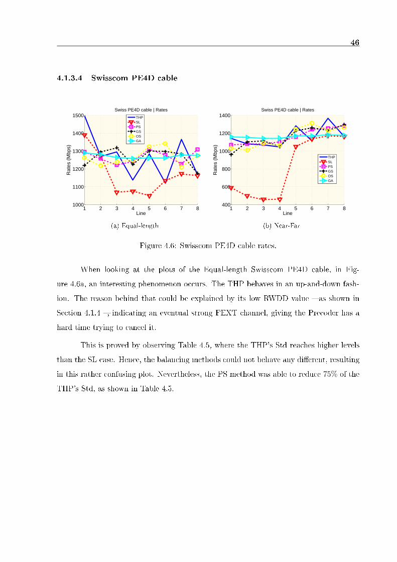
46

4.1.3.4 Swisscom PE4D cable

1 2 3 4 5 6 7 81000

1100

1200

1300

1400

1500Swiss PE4D cable | Rates

Line

Rat

es (

Mbp

s)

THPSLPSGSOSGA

(a) Equal-length

1 2 3 4 5 6 7 8400

600

800

1000

1200

1400Swiss PE4D cable | Rates

LineR

ates

(M

bps)

THPSLPSGSOSGA

(b) Near-Far

Figure 4.6: Swisscom PE4D cable rates.

When looking at the plots of the Equal-length Swisscom PE4D cable, in Fig-

ure 4.6a, an interesting phenomenon occurs. The THP behaves in an up-and-down fash-

ion. The reason behind that could be explained by its low RWDD value – as shown in

Section 4.1.4 –, indicating an eventual strong FEXT channel, giving the Precoder has a

hard time trying to cancel it.

This is proved by observing Table 4.5, where the THP’s Std reaches higher levels

than the SL case. Hence, the balancing methods could not behave any different, resulting

in this rather confusing plot. Nevertheless, the PS method was able to reduce 75% of the

THP’s Std, as shown in Table 4.5.

47

Equal length Near-Far

SL THP PS GS OS GA SL THP PS GS OS GA

Sum (Gbps) 9.33 10.14 10.14 10.11 10.12 10.17 6.52 9.26 9.27 9.24 9.24 9.29

Std (Mbps) 115.59 126.29 35.93 50.70 47.76 11.71 340.45 111.27 88.46 116.34 118.44 13.86

Max (Gbps) 1.39 1.50 1.31 1.32 1.34 1.29 1.17 1.36 1.28 1.29 1.31 1.18

Min (Gbps) 1.05 1.12 1.22 1.18 1.21 1.26 0.46 1.05 1.07 0.96 1.01 1.14

ET (ms) 0.10 0.22 0.19 3.92 0.17 1642.79 0.10 0.22 0.19 3.96 0.19 1639.13

Table 4.5: Swisscom PE4D cable rates.

An interesting fact happens in the Near-Far case. Whereas Figure 4.6b shows that

the balancing methods reside in approximately the same area of the THP, the GS and

OS methods yielded bigger Stds than the THP one. That confirms that more adaptation

of these methods must be done in order to achieve better rate-balancing for this cable,

which seem to be feasible, as shown by the low Std rate of the GA. Nonetheless, the

PS method was able to diminish the THP’s Std in the same processing time as the OS

method. In this cable, in particular, the GA-Sorting achieved results of 90.72% of Std

reduction for the Equal length case and of 87.54% for the Near-far case, meaning it was

the best method, if not considering the total processing time.

4.1.3.5 Swisscom I51 cable

Another cable to compare rates is the Swisscom I51. This cable shows one more

time a situation where the THP’s Std reaches higher levels than those of SL in the Equal-

length case – almost 200% –, however, the balancing methods were able to achieve positive

results (Table 4.6). For example, the GS method got close to the GA’s result, that achieved

95.79% of Std reduction. Like before, the GS method needs more time to process each

sorting, so its usage in this case must be done where the processing time is no potential

concern. Otherwise, both PS and OS methods stayed close to each other, what could be

a choice for the implementer.

The GS method repeated its performance in the Near-Far scenario, by reducing

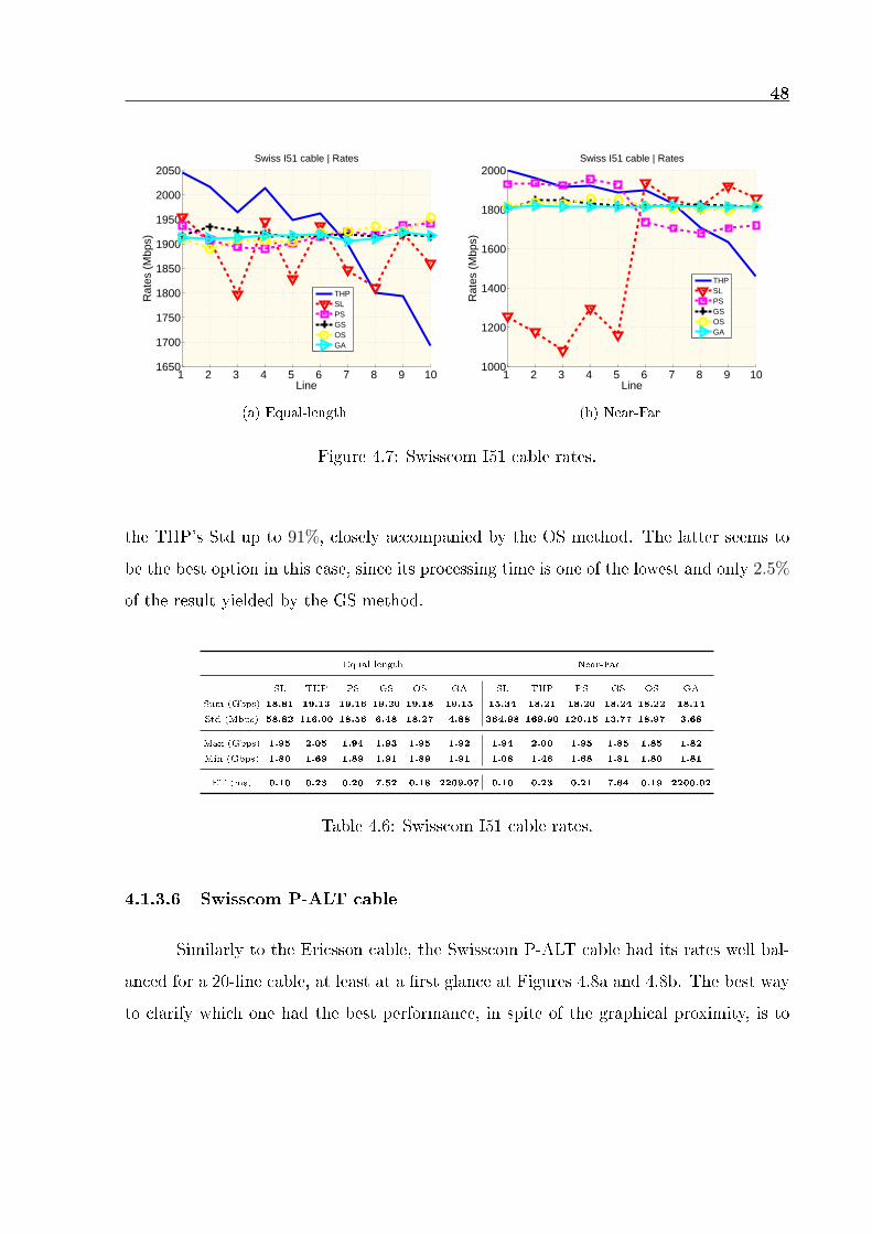
48

1 2 3 4 5 6 7 8 9 101650

1700

1750

1800

1850

1900

1950

2000

2050Swiss I51 cable | Rates

Line

Rat

es (

Mbp

s)

THPSLPSGSOSGA

(a) Equal-length

1 2 3 4 5 6 7 8 9 101000

1200

1400

1600

1800

2000Swiss I51 cable | Rates

Line

Rat

es (

Mbp

s)

THPSLPSGSOSGA

(b) Near-Far

Figure 4.7: Swisscom I51 cable rates.

the THP’s Std up to 91%, closely accompanied by the OS method. The latter seems to

be the best option in this case, since its processing time is one of the lowest and only 2.5%

of the result yielded by the GS method.

Equal length Near-Far

SL THP PS GS OS GA SL THP PS GS OS GA

Sum (Gbps) 18.81 19.13 19.16 19.20 19.18 19.15 15.34 18.21 18.20 18.24 18.22 18.14

Std (Mbps) 58.82 116.00 18.56 6.48 18.27 4.88 364.98 169.90 120.15 13.77 18.97 3.68

Max (Gbps) 1.95 2.05 1.94 1.93 1.95 1.92 1.94 2.00 1.95 1.85 1.85 1.82

Min (Gbps) 1.80 1.69 1.89 1.91 1.89 1.91 1.08 1.46 1.68 1.81 1.80 1.81

ET (ms) 0.10 0.23 0.20 7.52 0.18 2209.07 0.10 0.23 0.21 7.64 0.19 2200.02

Table 4.6: Swisscom I51 cable rates.

4.1.3.6 Swisscom P-ALT cable

Similarly to the Ericsson cable, the Swisscom P-ALT cable had its rates well bal-

anced for a 20-line cable, at least at a first glance at Figures 4.8a and 4.8b. The best way

to clarify which one had the best performance, in spite of the graphical proximity, is to

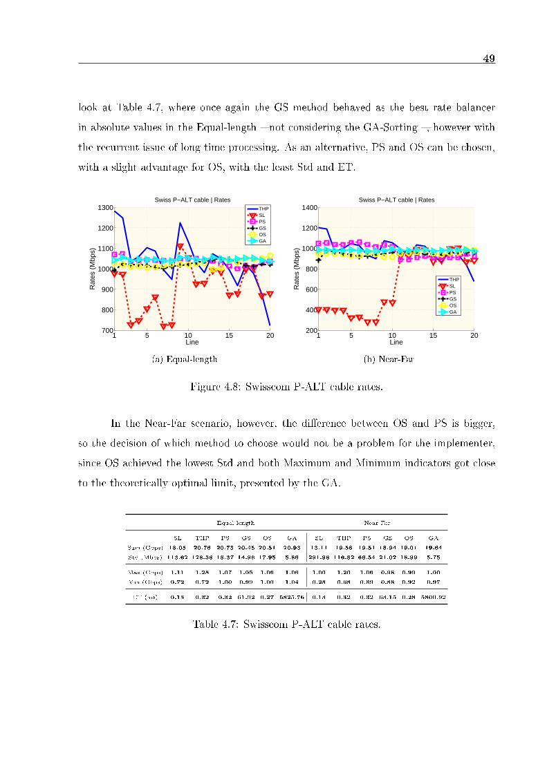
49

look at Table 4.7, where once again the GS method behaved as the best rate balancer

in absolute values in the Equal-length – not considering the GA-Sorting –, however with

the recurrent issue of long time processing. As an alternative, PS and OS can be chosen,

with a slight advantage for OS, with the least Std and ET.

1 5 10 15 20700

800

900

1000

1100

1200

1300Swiss P−ALT cable | Rates

Line

Rat

es (

Mbp

s)

THPSLPSGSOSGA

(a) Equal-length

1 5 10 15 20200

400

600

800

1000

1200

1400Swiss P−ALT cable | Rates

Line

Rat

es (

Mbp

s)

THPSLPSGSOSGA

(b) Near-Far

Figure 4.8: Swisscom P-ALT cable rates.

In the Near-Far scenario, however, the difference between OS and PS is bigger,

so the decision of which method to choose would not be a problem for the implementer,

since OS achieved the lowest Std and both Maximum and Minimum indicators got close

to the theoretically optimal limit, presented by the GA.

Equal length Near-Far

SL THP PS GS OS GA SL THP PS GS OS GA

Sum (Gbps) 18.05 20.76 20.73 20.45 20.51 20.93 13.11 19.58 19.51 18.94 19.01 19.64

Std (Mbps) 113.62 128.38 18.37 14.96 17.95 5.86 291.98 116.82 66.54 21.02 18.99 5.75

Max (Gbps) 1.11 1.28 1.07 1.05 1.06 1.06 1.00 1.20 1.06 0.98 0.99 1.00

Min (Gbps) 0.72 0.72 1.00 0.99 1.00 1.04 0.28 0.68 0.89 0.88 0.92 0.97

ET (ms) 0.13 0.32 0.32 61.92 0.27 5825.76 0.13 0.32 0.32 63.15 0.28 5800.92

Table 4.7: Swisscom P-ALT cable rates.

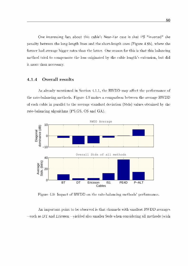
50

One interesting fact about this cable’s Near-Far case is that PS "inverted" the

penalty between the long-length lines and the short-length ones (Figure 4.8b), where the

former had average bigger rates than the latter. One reason for this is that this balancing

method tried to compensate the loss originated by the cable length’s extension, but did

it more than necessary.

4.1.4 Overall results

As already mentioned in Section 4.1.1, the RWDD may affect the performance of

the rate-balancing methods. Figure 4.9 makes a comparison between the average RWDD

of each cable in parallel to the average standard deviation (Stds) values obtained by the

rate-balancing algorithms (PS,GS, OS and GA).

−10

0

10RWDD Average

Dia

gona

ldo

min

ance

(dB

)

BT DT Ericsson I51 PE4D P−ALT0

20

40

Ave

rage

Std

s. (

bit/s

)

Cables

Overall Stds of all methods

Figure 4.9: Impact of RWDD on the rate-balancing methods’ performance.

An important point to be observed is that channels with smallest RWDD averages

– such as DT and Ericsson – yielded also smaller Stds when considering all methods (with

51

an exception to PE4D). This is the confirmation that the RWDD is a good approach when

dealing with measured cables and should be considered in this kind of simulations.

Chapter 5

CONCLUSION AND FURTHER

WORKS

Since the G.fast standard has been published, many efforts have been made for

achieving a better QoS. In this context, Vectoring has been in the center of today’s G.fast

researches due to its efficient capability of crosstalk cancellation. One of the main issues to

be faced is how equal the data is delivered to all users connected to the same multiplexer.

This work drew the attention to this matter and proposed a means of circumventing this

problem by applying mathematical procedures on the channel matrix, aiming at sorting

its columns, which resemble the direct channel of each line and the crosstalk they receive

and cause to lines of the same binder. Results showed that the proposed rate-balancing

methods (Post-sorting, GS-Sorting, Original Sorting and GA-Sorting) were able to deliver

promising results regarding rate-balancing of all users with some cables having better

results than others. That means that these methods still need a deeper investigation with

respect to optimizations, testing, simulations that can adapt to any cable for a future

deployment in the industry.

52

53

5.1 Further work

The investigation in rate-balancing will continue to develop, trying to keep pace

with new findings that come out every day, and being sure that this study field still has

a lot of potential to be explored. All results achieved in this work deal solely with rate-

balancing and could be surely enhanced by the collaboration of other techniques such

as Bonding, a practice able of increasing available capacity. This technique consists in

combining two VDSL2 lines to double the available bitrate, therefore delivering the same

rates to subscribers over long distances. The usage of both techniques together could

potentially increase the network performance in G.fast in the same way it is already being

used in VDSL2.

Bibliography

[1] Broadbandtrends, “VDSL2 with Vectoring,” Available at: http:

//broadbandtrends.com/blog1/wp-content/uploads/2012/11/VDSL2Vectored-

Ports1.jpg.

[2] Wikipedia, “Differences between SISO, SIMO, MISO and MIMO,” Available at:

http://commons.wikimedia.org/wiki/File:Prinzip_MIMO.png.

[3] Alcatel-Lucent, “G.fast uses very high frequencies to significantly increase bit rates on

very short loops,” Available at: http://www2.alcatel-lucent.com/techzine/the-

numbers-are-in-vectoring-2-0-makes-g-fast-faster/print-47/.

[4] Wikimedia, “FTTX,” Available at: http://upload.wikimedia.org/wikipedia/

commons/thumb/9/9e/FTTX.svg/300px-FTTX.svg.png.

[5] Troy Wolverton, “DSL speed could soon get a boost with new technologies,” Avail-

able at: http://www.mercurynews.com/ci_22998468/new-technologies-your-

dsl-speed-could-soon-get.

[6] R. Zidane, S. Huberman, C. Leung, and Tho Le-Ngoc, “Vectored DSL: benefits and

challenges for service providers,” Communications Magazine, IEEE, vol. 51, no. 2,

pp. 152–157, February 2013.

54

55

[7] ITU-T Recommendation G.993.5, “Self-FEXT cancellation (vectoring) for use

with VDSL2 transceivers,” International Telecommunication Union recommendation,

2010.

[8] Hermann Lipfert, “MIMO OFDM Space Time Coding - Spatial Multiplexing, In-

creasing Performance and Spectral Efficiency in Wireless Systems,” Tech. Rep.

Part I Technical Basis, Institut für Rundfunktechnik, 2007, Available at: http:

//www.irt.de/webarchiv/showdoc.php?z=OTAyIzEwMDYwMTMxMCNwZGY=.

[9] A. Sibille, C. Oestges, and A. Zanella, MIMO: From Theory to Implementation, p.

195, Elsevier Science, 2010.

[10] P. Odling, T. Magesacher, S. Host, P.O. Borjesson, M. Berg, and E. Areizaga, “The

fourth generation broadband concept,” Communications Magazine, IEEE, vol. 47,

no. 1, pp. 62–69, January 2009.

[11] ITU-T Recommendation G.9700, “Fast access to subscriber terminals (G.fast) -

Power spectral density specification,” International Telecommunication Union, 2014.

[12] ITU-T Recommendation G.9701, “Fast access to subscriber terminals (G.fast) -

Physical layer specification,” International Telecommunication Union, 2014.

[13] Frank Van der Putten, “Overview of G.fast: Summary overview and timeline,” Tech.

Rep., 2014.

[14] Alcatel-Lucent, “The Numbers are in: Vectoring 2.0 Makes G.fast Faster,”

Available at: http://www2.alcatel-lucent.com/techzine/the-numbers-are-

in-vectoring-2-0-makes-g-fast-faster/.

[15] LightReading, “Sckipio Unveils G.fast Chipsets,” Available at: http:

//www.lightreading.com/broadband/dsl-vectoring-gfast/sckipio-unveils-

gfast-chipsets/d/d-id/711304?

56

[16] Tim Verry, “G.fast Delivers Gigabit Broadband Speeds To Customers Over Cop-

per (FTTdp),” Available at: http://www.pcper.com/news/General-Tech/GFast-

Delivers-Gigabit-Broadband-Speeds-Customers-Over-Copper-FTTdp.

[17] W. Ford, Numerical Linear Algebra with Applications: Using MATLAB, Elsevier

Science, 2014.

[18] A. Greenbaum and T.P. Chartier, Numerical Methods: Design, Analysis, and Com-

puter Implementation of Algorithms, p. 169, Princeton University Press, 2012.

[19] Ward Cheney and David Kincaid, Linear Algebra: Theory and Applications, pp.

544,558, Sudbury, MA, USA: Jones & Bartlett Learning, 2009.

[20] L.N. Trefethen and D. Bau, Numerical Linear Algebra, pp. 48–49, Society for Indus-

trial and Applied Mathematics (SIAM, 3600 Market Street, Floor 6, Philadelphia,

PA 19104), 1997.

[21] J. G. F. Francis, “The QR transformation A unitary analogue to the LR transforma-

tion - part 1,” The Computer Journal, vol. 4, no. 3, pp. 265–271, 1961.

[22] J. G. F. Francis, “The QR transformation - part 2,” The Computer Journal, vol. 4,

no. 4, pp. 332–345, 1962.

[23] Beresford N. Parlett, “The QR algorithm,” Computing in Science and Engg., vol. 2,

no. 1, pp. 38–42, Jan. 2000.

[24] V. Oksman, H. Schenk, A. Clausen, J.M. Cioffi, M. Mohseni, G. Ginis, C. Nuzman,

J. Maes, M. Peeters, K. Fisher, and P.-E. Eriksson, “The ITU-T’s New G.vector

Standard Proliferates 100 Mb/s DSL,” Communications Magazine, IEEE, vol. 48,

no. 10, pp. 140–148, October 2010.

[25] M. Tomlinson, “New automatic equaliser employing modulo arithmetic,” Electronics

Letters, vol. 7, no. 5, pp. 138–139, March 1971.

57

[26] H. Harashima and H. Miyakawa, “Matched-transmission technique for channels with

intersymbol interference,” Communications, IEEE Transactions on, vol. 20, no. 4,

pp. 774–780, Aug 1972.

[27] R. Cendrillon, G. Ginis, E. Van den Bogaert, and M. Moonen, “A near-optimal linear

crosstalk precoder for downstream VDSL,” Communications, IEEE Transactions on,

vol. 55, no. 5, pp. 860–863, May 2007.

[28] British Telecom, “G.fast: Release of BT cable measurements for use in simulations,”

Geneva, Switzerland: Contribution ITU-T 2013-01-Q4-066, 2013.

[29] G. Ginis and J.M. Cioffi, “A multi-user precoding scheme achieving crosstalk cancel-

lation with application to DSL systems,” vol. 2, pp. 1627–1631 vol.2, Oct 2000.

[30] G. Ginis and J.M. Cioffi, “Vectored transmission for digital subscriber line systems,”

Selected Areas in Communications, IEEE Journal on, vol. 20, no. 5, pp. 1085–1104,

Jun 2002.

[31] R. Cendrillon, M. Moonen, J. Verlinden, T. Bostoen, and G. Ginis, “Improved linear

crosstalk precompensation for DSL,” in Acoustics, Speech, and Signal Processing,

2004. Proceedings. (ICASSP ’04). IEEE International Conference on, May 2004,

vol. 4, pp. iv–1053–6 vol.4.

[32] D. Torrieri, Principles of Spread-Spectrum Communication Systems, Second Edition,

p. 348, SpringerLink : Bücher. Springer, 2011.

[33] V.J. Arokiamary, Mobile Communications, p. 3.57, Technical Publications, 2009.

[34] B. Ram, Engineering Mathematics, p. 13.63, Pearson Education, 2009.

[35] J. M. Cioffi, “Course notes for EE379A - digital communication,” Stanford University,

Available at: http://web.stanford.edu/group/cioffi/ee379a/course_reader/

chap3.pdf.

58

[36] ASSIA, “G.fast: Non-Linear Precoder Ordering,” ITU-T Study Group 15 - Contri-

bution 0261.

[37] International Telecommunication Union, “Access to documents,” Available at: http:

//www.itu.int/en/ITU-T/ewm/Pages/documents-access.aspx.

[38] S. Theodoridis and R. Chellappa, Academic Press Library in Signal Processing:

Communications and Radar Signal Processing, pp. 301–302, Academic Press Library

in Signal Processing. Elsevier Science, 2013.