Presenting and corresponding author: MSc, Luis A. Mejia Camones

Simulation of the hydraulic fracturing processes combining finite

elements and lattice Boltzmann methods

Luis A. Mejia Camones1, E. Vargas Jr.2, R. Velloso3, G. H. Paulino4

1Pontifical Catholic University of Rio de Janeiro, luisarnaldo@puc-rio.br 2 Pontifical Catholic University of Rio de Janeiro, vargas@puc-rio.br

3 Federal University of Ouro Preto, rqvelloso@gmail.com 4 University of Illinois at Urbana-Champaign, paulino@illinois.edu

Abstract This research addresses hydraulic fracturing or hydro-fracking, i.e. fracture propagation process in rocks through the injection of a fluid under pressure, which generates cracks in the rock that propagate according to the amount of fluid injected. This technique leads to an increase of the permeability of the rock mass and consequently improve oil production. Several analytical and numerical models have been proposed to study this fracture mechanism, generally based in continuum mechanics or using interface elements through a known propagation path. In this work, the crack propagation is simulated using the PPR potential-based cohesive zone model [1,2] by means of an extrinsic implementation. Thus, interface cohesive elements are adaptively inserted in the mesh to capture the softening fracture process. The fluid pressure is simulated using the lattice Boltzmann model [3] through an iterative procedure. The boundaries of the crack, computed using the finite element method, are transferred to the lattice Bolztmann model as boundary conditions, where the force applied on these boundaries, caused by the fluid pressure, can be calculated. These forces are then transferred to the finite element model as external forces applied on the faces of the crack. The new position of the crack faces is then calculated and transferred to the lattice Boltzmann model to update the boundary conditions. This feedback-loop for fluid-structure interaction allows modeling of hydraulic fracturing processes. Examples will be provided to demonstrate the features of the proposed methodology.

Keywords: Lattice Boltzmann, PPR Model, hydraulic fracturing, crack propagation.

1. Introduction

In hydraulic fracturing process, a discontinuity is created inside a solid through the application of hydraulic pressure. To create a crack, the fluid pressure injected has to be higher than the sum between the tensile strength and the minor confined stress. The crack propagation happens when the fluid injected flows into the crack. Several applications of this process may be observed in different areas (civil, mining and oil industries) having their most relevant application in oil industry [4]. To improve the oil production, hydraulic fracturing process is used to create cracks inside the rock reservoir, increasing the permeability. Several authors have studied the hydraulic fracturing process from analytical [5-7] and numerical [8-10] perspective, generally based in continuum mechanics or using interface elements through a known propagation path. The hydraulic fracturing process is a coupled phenomenon that involves a moving boundary and fluid flow into the fractures, where the fluid flow depends of the crack aperture. When the material has heterogeneities or discontinuities, a fracture could be propagated in an irregular path, showing branching. Conventional finite element method (FEM) does not easily allow simulating irregular crack propagation. The use of enrichment elements can become a difficult task to be implemented when the fracture has an irregular path or show branching. Otherwise, interface elements used to represent the nonlinear fracture process zone ahead of a crack tip, allow simulating these irregular paths and their implementation may be easier than the enrichment elements. The interface elements can be inserted into the mesh at the beginning of the calculation process (intrinsic) or inserted into the mesh to capture the softening process fracture (extrinsic). The softening fracture process is modeled by the interface elements and the crack is considered opened when their aperture reach a critical value.

A fluid flow into an interface element (crack) may be considered as a flow between parallels plates, where its motion can

be described by the Navier-Stokes equations. An alternative method to solve these equations is the lattice Boltzmann method (LBM) [11-13]. This method allows simulating the fluid flow through complex geometries as a fracture.

The proposal of this research is simulating the hydraulic fracturing process using the FEM coupled with the LBM.

PPR potential-based cohesive model implementation to simulate the crack propagation.

Finite element method (FEM) is used to simulate the mechanical process of the hydraulic fracturing. The crack propagation is modeled using the PPR potential-based cohesive model [1,2] by means of an extrinsic implementation. In this case, the cohesive elements are adaptively inserted in the mesh to capture the softening process. The consequence of this insertion is the duplication of some nodes during the calculation process. To manage the mesh information and the changes in its topology we use the Tops code [14,15]. The Tops code is a topological data framework developed in C++ that supports these modifications in the mesh and allows optimum information management. To insert the cohesive elements, the tensile traction is checked at all facets of the mesh and is inserted when this tensile traction supersedes the normal or tangential cohesive strengths. The cohesive element allows simulating the softening process through the cohesive traction-separation relationship [2] given by:

(1)

Where is the potential function for cohesive element, are the normal and tangential cohesive strengths, are the energy constant in the PPR model, are the separation field in local coordinates, are the normal and tangential final crack opening widths and are the shape parameters in PPR model. The gradient of the PPR potential leads to the normal and tangential cohesive tractions along the fracture surface by:

(2)

(3)

The finite element code implemented uses linear triangular elements (T3) and the cohesive element is composed of 4 nodes. 2. Fluid flow simulation using the lattice Boltzmann model.

Fluid modeling may be accomplished by using the LBM. In this model, space is discretized in cells where the probable number of particles that comprise them, (on time and with velocity v) is represented by the distribution function . From this function, fluid macroscopic variables may be calculated. Usually, the solution of LBM is accomplished via two-step process of collision and propagation. The collision phase redistributes the particles on the node (particles collide with each other) due to the collision effect and the propagation phase propagates the particles to neighboring nodes. For each step, the collision process is given by:

(4)

and the propagation process, by:

(5)

Where the , is the time relaxation, is the equilibrium distribution function, is the position of the node and is the time. For the two-dimensional case, it is usual to choose a D2Q9 cell that allows nine velocity directions, four on the vertex of the cell, four at the center of each cell side and one in the center of the cell itself. The solids can be included in

Ψ(Δn,Δt ) =min(Φn,Φt )+ Γn 1-Δn

δn

%

&'

(

)*

α

+ Φn -Φ t

+

,--

.

/00Γt 1-

Δt

δt

%

&'

(

)*

β

+ Φ t -Φn

+

,--

.

/00

Ψ Φn,Φ t Γn,ΓtΔn,Δt δn,δt

α,β

Tn (Δn,Δt ) = −αΓn

δn1- Δn

δn

$

%&

'

()

α−1

Γt 1-Δt

δt

$

%&

'

()

β

+ Φ t -Φn

+

,--

.

/00

Tt (Δn,Δt ) = −βΓt

δt1-

Δt

δt

$

%&

'

()

β−1

Γn 1-Δn

δn

$

%&

'

()

α

+ Φn -Φ t

+

,--

.

/00

Δt

Δt

t f (x,v, t)

fα' (x, t) = fα (x, t)−

1τ *( fα (x, t)− fα

eq (x, t))

fα (x + vαΔt, t +Δt) = fα' (x, t)

τ * = τ /Δt τ f eq xt

the mesh. Each cell is identified with a number: “one” for solids and “zero” for fluids. Considering as the distance from the boundary (interface solid-liquid) to some neighbor node, the bounce-back condition is considered when . In this case, the boundary is located at the middle distance between two nodes and the particles are reflected in the same direction from where they came. For other boundary locations, interpolation functions are used to calculate the value of the distribution function [12]. For the case when , the value of the distribution function reflected from the boundary ( ) is given by:

(6)

when , the same function is given by:

(7)

Where represent the position of the neighbor node to the node at the direction [12]. This research does not consider the fluid penetration into the solid. 3. Coupling implementation and first results. Two meshes are used in the coupling process between FEM and LBM. The fracture boundaries are obtained from the finite

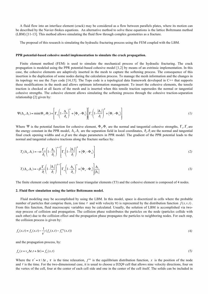
element mesh. Their position, which is computed using FEM, are transferred to the LBM. The force applied on the boundaries, caused by the fluid pressure, can be computed using LBM. After this calculation, these forces are transferred to the FEM and applied as external forces on the faces of the crack. The new position of the crack boundaries is calculated using FEM and then is transferred to the LBM to update the boundary conditions. Similar to the coupling process between the discrete element method (DEM) and LBM [3,16], the coupling process between FEM and LBM has two time steps. Normally, the time step for the FEM is smaller than the time step for the LBM. For this feedback-loop for fluid-structure interaction, it is necessary to define a subcycle number. The subcycle number can be described by:

(8) where n(subcycle) is an integer number, Δt is the LBM time step and dt is the FEM time step. Thus, for one step in lattice Boltzmann ,“n” steps of FEM are needed.

Figure 1. a) The coupling process between FEM and LBM for each subcycle; b) Detail of the two meshes used on the numerical simulation. The LB mesh is created in the zone where the fracture propagation happens. An example of the coupling process between FEM and LBM and the properties of the material, fluid and characteristics of the meshes are showed in figure 2. A fluid pressure is applied to a portion of the notch. Using the LBM, the magnitude of the forces developed at the boundaries is calculated and transferred to the FEM. Because of the application of these forces, the boundaries move and their new position are transferred to the LBM to update the boundary condition. In this example, the fluid applied a pressure on the initial crack faces but did not flow into the crack. Nevertheless, it is possible to see the crack

qq =1/ 2

q <1/ 2 α

fα(rj, t) = q(1+ 2q) fα (rj + eαδt, t)+ (1− 4q

2 ) fα (rj, t)− q(1− 2q) fα (rj − eαδt, t)+3wα (eα.uw )

q >1/ 2

fα(rj, t) =

1q(2q+1)

fα (rj + eαδt, t)+2q−1q

fα(rj − eαδt, t)−

(2q−1)(2q+1)

fα(rj − 2eαδt, t)+

3wα

q(2q+1)(eα.uw )

rj ± eαδt rj eαδt

n(subcycle) ≈ Δt / dt +1

Fluid ModelLB

Forces(applied on the

boundaries)

Mechanical ModelFEM

(apply the forces on theboundaries)

update boundaries

FEM mesh

LB mesh

crack( )cohesive element

FEM mesh

LB mesh

crack propagated(full opening crack)

Boundary (LB mesh)

Update boundary (LB mesh)

solid fluid

FEM-LB coupling (update boundary-scheme)

a) b)

coupling process

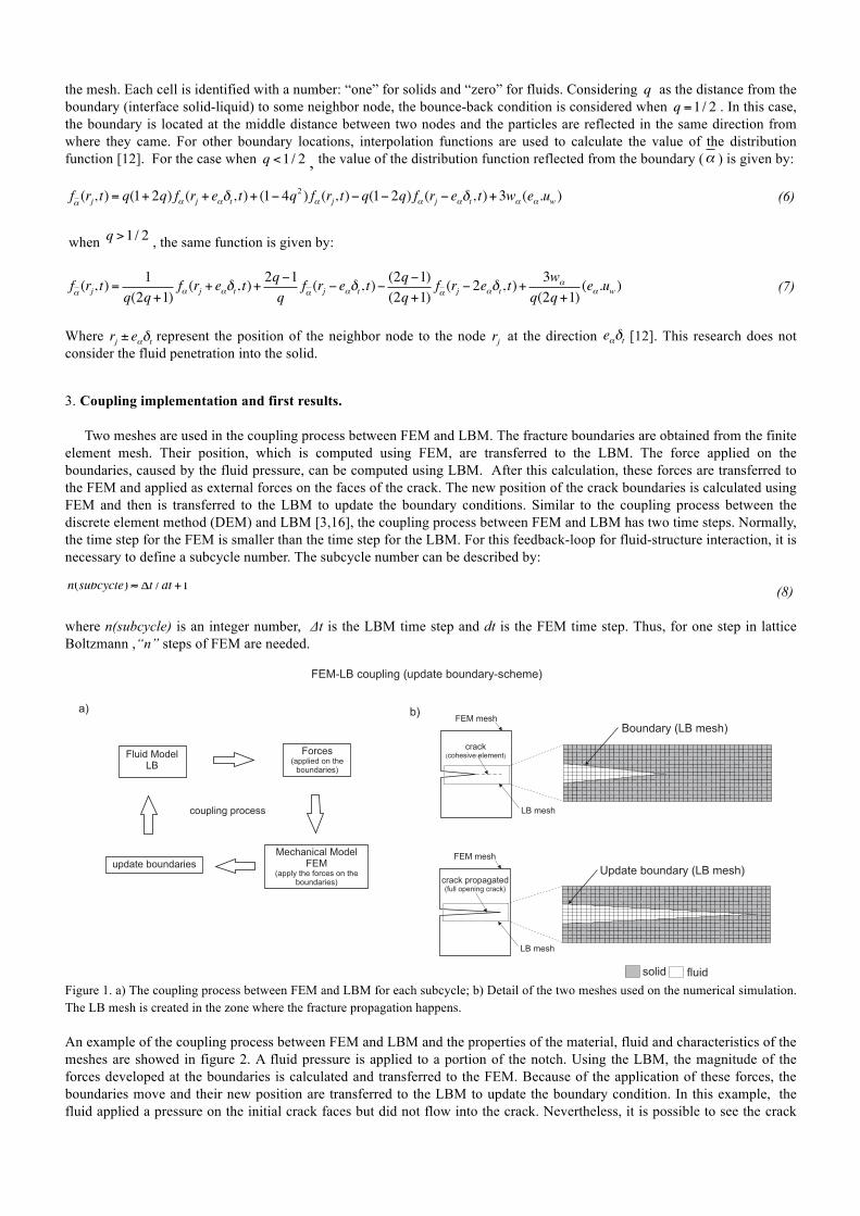
propagation.

Figura 2. a) Description of the meshes and properties of the material and fluid. b) crack propagation caused by the fluid pressure. 4. Conclusions. This paper presented the methodology developed to execute the coupling between FEM and LBM. The PPR model was used by means the extrinsic implementation. The cohesive elements are adaptively inserted in the mesh to capture the softening process, and the crack propagation may be simulated for regular or irregular path. The LBM is used to simulate the fluid flow. Considering the fluid flow into the crack as a flow into parallel plates, the Navier-Stokes equations may be solved using LBM. The FEM-LBM coupling allows simulating the hydraulic fracturing due to the advantage of the LBM to simulate the fluid flow in complex boundary conditions, as a fracture. Acknowledgements

The author thanks to the CAPES Foundation of the Ministry of Education of Brazil by the financial funding for this research. Proc. 12144/13-4. References 1. K. Park, G. H. Paulino, 2012. Computational implementation of the PPR potential-based cohesive model in ABAQUS: Educational perspective, Engineering Fracture Mechanics, 93, 239-262. 2. K. Park, G. H. Paulino, J. Roesler, 2009. A unified potential-based cohesive model of mixed mode fracture, Journal of the Mechanics and Physics of Solids, 57, 891-908. 3. R. Velloso, 2010. Numerical analysis of fluid mechanical coupling in porous media using the discrete element method, PhD dissertation, Pontifical Catholic University of Rio de Janeiro (in Portuguese). 4. M. Hunsweeck, Y. Shen, A. Lew, 2012. A finite element approach to the simulation of the hydraulic fractures with lag. International Journal for Numerical and Analytical Methods in Geomechanics, 37, 993-1015. 5. J. Adachi, E. Detoournay, 2008. Plane strain propagation of a hydraulic fracture in a permeable rock. Engineering Fracture Mechanics, 75(16):4666-94. 6. A Burger, E. Detournay, E. Garagash, 2005. Toughness-dominated hydraulic fractured with leak-off. International Journal of Fracture, 134(2): 175-90. 7. E. Detournay, 2004. Propagation regimes of fluid-driven fractures in impermeable rocks. International Journal of Geomechanics, 4: 35-45. 8. M. Hunsweck, Y. Shen, , A. Lew, 2012. A finite element approach to the simulation of hydraulic fractures with lag. International Journal for Numerical and Method in Geomechanics. 37: 993-1015. 9. B. Carrier, S. Granet, 2012. Numerical modeling of hydraulic fracture problem in permeable medium using cohesive zone model. Engineering Fracture Mechanics. 79: 312-328. 10. B. Lecampion, 2009. An extended finite element method for hydraulic fracture problems. Communications in Numerical Methods in Engineering. 25: 121-133. 11. G. McNamara, G. Zanetti, 1988. Use the Boltzmann equation to simulate lattice-gas automata. Physics Review, 61: 2332. 12. P. Lallemand, L. Luo, 2003. Lattice Boltzmann method for moving Boundaries. Journal of Computational Physics, 184: 406-421. 13. D. R. Noble, J. R. Torczynsky, 1998. A lattice Boltzmann method for partially saturated computational cells. International Journal of Modern Physics. 9(8): 1189-1201. 14. G, Paulino, W. Celes, R. Espinha, Z. Zhang, 2008. A general topology-based framework for adaptive insertion of cohesive element in finite element meshes. Engineering with Computers, 24: 59-78. 15 R. Espinha, W. Celes, N. Rodrigues and G. Paulino, 2009. Partops: compact topological framework for parallel fragmentation simulations. Engineering with computers, 25(4): 345-365. 16. K. Han, Y. Feng, D. Owen, 2007. Coupled lattice Boltzmann and discrete element modeling of fluid-particle interaction problems. Computers & Structures, 85: 1080-1088.

50mm

50mm25mm

5mm

2.5mm

fluid

Mesh (FEM)

Material properties

1708 Nodes3316 Elementsdt = 4.4e-9s

E=50GPa=0.25

G=50J/m=5MPa

ν

σf

t

2

Mesh (LBM)

Fluid properties

35000 cells35000 lattice nodes

t=1.0e-6sx=1.0e-5m

visc=2.0e-6m /s

P=15MPa

ΔΔ

ρ=1000kg/m

2

3

P

a)b)

crack propagation