relatórios científicos e técnicos ipma, série digital, 2

RELATÓRIOS CIENTÍFICOS E TÉCNICOS DO IPMA – SÉRIE DIGITAL

Destinam-se a promover uma divulgação rápida de resultados de carácter científico e técnico, resultantes da actividade de investigação e do desenvolvimento e inovação tecnológica nas áreas de investigação do mar e da atmosfera. Esta publicação é aberta à comunidade científica e aos utentes, podendo os trabalhos serem escritos em Português, Francês ou Inglês.

Edição IPMA

Rua C – Aeroporto de Lisboa 1749-007 LISBOA

Portugal

Corpo Editorial

Francisco Ruano – Coordenador

Aida Campos

Irineu Batista

Lourdes Bogalho

Mário Mil-Homens

Rogélia Martins Teresa Drago

Edição Digital Anabela Farinha / Luis Catalan

As instruções aos autores estão disponíveis no sitio web do IPMA

http://ipma.pt/pt/publicacoes/index.jsp

ou podem ser solicitadas aos membros do Corpo Editorial desta publicação

Capa

Luis Catalan

ISSN

2183-2900

Todos os direitos reservados

http://www.ipma.pt/pt/publicacoes/index.jsp

Workshop on Sampling Design and Optimization - WKSDO

IPMA, 17-20 November 2014

Report of the Workshop on Sampling Design and Optimization of fisheries

data - WKSDO

Manuela Azevedo, Cristina Silva, Jon Helge Vølstad, Nuno Prista, Ricardo Alpoim,

Teresa Moura, Ivone Figueiredo, Marina Dias, Ana Cláudia Fernandes, Pedro G. Lino,

Mónica Felício, Corina Chaves, Eduardo Soares, Sandra Dores, Patrícia Gonçalves, Ana

Maria Costa and Cristina Nunes

IPMA - Divisão de Modelação e Recursos da Pesca (DivRP) Av. Brasília, 1449-006 Lisboa

Recebido em 2014-12-15 Aceite em 2014-12-19

RESUMO

Título: Relatório do workshop sobre o planeamento da amostragem e optimização de dados da pesca

O “Workshop on Sampling Design and Optimization (WKSDO)”, presidido pelas investigadoras Cristina

Silva e Manuela Azevedo (IPMA) e o investigador Norueguês Jon H. Vølstad (IMR), decorreu no IPMA-

Algés, de 17 a 20 de Novembro de 2014, para analisar o actual Programa Nacional de Amostragem Biológica

(PNAB/Data Collection Framework) com o objectivo de optimizar o programa de amostragem em lota para

estimação da composição por comprimento da captura/desembarque das espécies capturadas pela frota

nacional, de amostragem das capturas a bordo e da amostragem biológica para estudos de crescimento e

reprodução. O Workshop, organizado no âmbito do projecto de investigação nacional GesPe (Planos de

Gestão Pesqueira, PROMAR) e do PNAB/DCF, foi planeado e calendarizado tendo em conta o início do

processo de revisão do programa Europeu de recolha de dados da pesca de suporte à avaliação e gestão dos

recursos pesqueiros (DFC). Foram analisados e discutidos vários métodos e abordagens que resultaram num

conjunto de instruções e recomendações para trabalho futuro, relevantes para assegurar uma elevada

qualidade e optimização do futuro programa de amostragem.

Palavras chave: Amostragem a bordo, Amostragem em lota, Chaves comprimento-idade, Ogiva de

maturação, Programa Nacional de Amostragem Biológica.

ABSTRACT

The Workshop on Sampling Design and Optimization (WKSDO), chaired by Cristina Silva and Manuela

Azevedo (IPMA-PT) and Jon H. Vølstad (IMR-NO) met in Lisbon, 17–20 November 2014, to focus on the

analysis of the current Portuguese sampling designs under PNAB/DCF (Programa Nacional de Amostragem

Biológica/Data Collection Framework) with the aim to optimize the current market sampling design to

estimate the species length composition of landings, the onboard sampling for catches and the biological

sampling for growth and maturity. The Workshop was organized within the scope of the national research

project - GesPe (Planos de Gestão Pesqueira, PROMAR) and the PNAB/DCF and the planning and timing of

the workshop took into account the initiated review process of EU fisheries data collection for stock

assessment and management (DCF - Data Collection Framework). During the workshop several approaches

and methods were analysed and discussed, resulting in a set of guidelines and recommendations for future

work which are relevant to ensure a high quality and optimized future data collection programme.

Key words: Age-length keys, Market sampling, Maturity ogive, National Biological Sampling Programme, Onboard

sampling.

REFERÊNCIA BIBLIOGRÁFICA

AZEVEDO, M.; SILVA, C.; VØLSTAD, J.H.; PRISTA, N.; ALPOIM, R.; MOURA, T.; FIGUEIREDO, I.; DIAS, M.; FERNANDES, A.C.; LINO, P. G.; FELÍCIO, M.; CHAVES, C.; SOARES, E.; DORES, S.; GONÇALVES, P.; COSTA, A.M.; NUNES, C. 2014. Report of the Workshop on Sampling Design and Optimization of fisheries data. Relat. Cient. Téc. do IPMA(http://ipma.pt), nº 2, 79 pp.

Table of Contents

1 Introduction .......................................................................................................................................................................... 6

1.1 Terms of reference ........................................................................................................................................................ 6

1.2 Background ................................................................................................................................................................... 6

1.3 Conduct of the meeting ............................................................................................................................................... 6

2 Market sampling for length composition (ToR 1) ...................................................................................................... 7

2.1 Background information and description of current sampling design ................................................................. 7

2.2 Analysis of current concurrent sampling program .................................................................................................. 8

2.3 Evaluation of the feasibility to accommodate concurrent sampling and sampling directed at trips that landed monkfish or skates and rays .............................................................................................................................. 12

2.4 Improving accuracy of estimated length composition .......................................................................................... 16

2.5 Discussion and conclusions ....................................................................................................................................... 17

3 On-board sampling for catches (ToR 2) .................................................................................................................... 18

3.1 Sampling designs ............................................................................................................................................... 18

3.1.1 Sampling design in Division IXa ....................................................................................................................... 18

3.1.2 Sampling design in the Indian Ocean ............................................................................................................... 20

3.2 Sources of bias on onboard sampling ...................................................................................................................... 20

3.2.1 Literature review ................................................................................................................................................. 20

3.2.2 Case study on Fish Otter Trawl (>=24m) .......................................................................................................... 21

3.3 Discussion and conclusions ....................................................................................................................................... 24

4 Sampling for biological parameters – Growth and Reproduction (ToR 3) ........................................................... 25

4.1 Age-length Keys ......................................................................................................................................................... 25

4.1.1 Sampling effort: how much is enough? ............................................................................................................ 25

4.1.2 Sardine case-study .............................................................................................................................................. 26

4.2 Maturity ogives ........................................................................................................................................................... 34

4.2.1 Introduction to hake case-study ........................................................................................................................ 34

4.2.2 Improving the estimation of maturity ogive ................................................................................................... 34

4.3 Discussion and Conclusions...................................................................................................................................... 37

4.3.1 Growth .................................................................................................................................................................. 37

4.3.2 Reproduction ....................................................................................................................................................... 38

5 Recommendations and Future Work ........................................................................................................................ 38

6 References ..................................................................................................................................................................... 40

Annex 1: List of participants ................................................................................................................................................ 41

Annex 2: Meeting Agenda ................................................................................................................................................... 43

Annex 3: Glossary of statistical terms ................................................................................................................................ 45

Annex 4: Presentations ......................................................................................................................................................... 48

- 6 -

1 1 1 1 IntroductionIntroductionIntroductionIntroduction

1.1 1.1 1.1 1.1 Terms of referenceTerms of referenceTerms of referenceTerms of reference

The Workshop on Sampling Design and Optimization (WKSDO), chaired by Cristina Silva and Manuela Azevedo (IPMA-PT) and Jon H. Vølstad (IMR-NO) took place in Lisbon, 17–20 November 2014, to focus on the analysis of the current Portuguese sampling designs under PNAB/DCF (Programa Nacional de Amostragem Biológica/Data Collection Framework) and their optimization:

1) Market sampling design to estimate the length composition of landings: concurrent sampling and species focus sampling.

2) On-board sampling for catches: objectives, sampling design, sampling effort, constraints, approaches for raising, improving the precision of estimates.

3) Sampling for biological parameters used in stock assessment.

1.2 1.2 1.2 1.2 BackgroundBackgroundBackgroundBackground

The Workshop was organized within the scope of the national research project - GesPe (Planos de Gestão Pesqueira, PROMAR) and the national biological sampling programme - PNAB/DCF.

1.3 1.3 1.3 1.3 Conduct of the meetingConduct of the meetingConduct of the meetingConduct of the meeting

The workshop participants made available several documents prepared in advance to the meeting, including a glossary of statistical terms to be used during the workshop (Annex 3), as well as several presentations (Annex 4) which subsequently formed the basis of the workshop’s investigations and discussions during the week.

The following speakers presented the talks indicated:

P01 - Manuela Azevedo: Portuguese Fleets and Fisheries. M. Azevedo, C. Silva, M. Dias

ToR 1) Market sampling design to estimate the length composition of landings: concurrent sampling and species focus sampling.

P02 - Nuno Prista: Present sampling design. N. Prista, M. Dias

P03 - Ricardo Alpoim: Anglerfishes. R. Alpoim, T. Moura, N. Prista

P04 - Ivone Figueiredo: Rays. I. Figueiredo, C. Maia

P05 - Manuela Azevedo: Catch length composition estimated from commercial size-categories: does it improve accuracy? M. Azevedo, C. Silva

P06 - Jon H. Vølstad: Sampling designs

ToR 2) On-board sampling for catches: objectives, sampling design, sampling effort, constraints, approaches for raising, improving the precision of estimates.

P07 - Ana Cláudia Fernandes: Sampling design in Div. IXa. A. C. Fernandes, N. Prista

P08 - Pedro Lino: Sampling design in Indian Ocean. P. G. Lino, R. Coelho, M. N. Santos

P09 - Jon Vølstad: Framework for assessing monitoring effort to support stock assessment.

ToR 3) Sampling for biological parameters used in stock assessment.

P10 - Jon Vølstad: Sampling/precision ALKs.

- 7 -

P11 - Eduardo Soares: Sampling for age / ALKs: sardine Case-study.

P12 - Ana Maria Costa: Sampling for maturity / maturity ogive: hake case-study. A. M. Costa, C. Nunes, J. Pereira

During the workshop the participants were divided into three subgroups dealing with each of the ToRs.

2222 Market sampling for length composition (ToR 1)Market sampling for length composition (ToR 1)Market sampling for length composition (ToR 1)Market sampling for length composition (ToR 1)

2.1 2.1 2.1 2.1 Background information and dBackground information and dBackground information and dBackground information and description of escription of escription of escription of current current current current sampling design sampling design sampling design sampling design

Market sampling for length composition in ICES Division IXa is carried out by IPMA and its design has evolved through time. Before 2009 the sampling plan was species-focused following the requirements of the former DCF (Commission Regulation (EC) No. 1639/2001). From 2009 onwards the design was changed to focus on métiers conforming new DCF requirements (Commission Decision No. 2010/93/UE). Following preparatory discussions on probability-based sampling held at the ICES Planning Group on Commercial Catches, Discards and Biological Sampling (PGCCDBS) and the Workshop on Practical Implementation of Statistical Sound Catch Sampling Programs (WKPICS), IPMA decided to test a new market sampling plan in 2014. This new sampling plan draws on the preparatory work carried out by several ICES Workshops and Study Groups dealing with sampling design (e.g. WKACCU, 2008; WKMERGE, 2010; SGPIDS, 2011-2013; WKPICS, 2011-2013; several PGCCDBS meetings) and available preparatory documents for the new DC-MAP where growing emphasis is put on the development of statistically sound probability-based sampling schemes that move away from previous quota sampling practices. The goal of the new sampling plan is therefore to improve the quality of data sent for ICES stock assessments and the overall quality of fisheries data collected from the Portuguese coast and its ecosystems.

The Portuguese fleet that operates in waters of ICES Division IXa comprises ~85 trawlers and ~115 purse-seiners (medium to large sizes) with the remainder (~6400 vessels) being considered “polyvalent” (Azevedo et al., P01 - Annex 4). The “polyvalent” fleet includes a large set of fishing vessels, highly variable in length (from a few meters to over 30 meters) and daily catch volume, and is typically multi-gear (i.e., each vessel can have more than one fishing license) and multi-species (i.e., individual vessels frequently target multiple species in each trip and/or throughout the year).

The Portuguese sampling design targeting fish lengths in 2014 is stratified multistage, with auction*day as the Primary Sampling Unit (PSU) and vessel landing events as the Secondary Sampling Unit (SSU). The PSUs are stratified by quarter and port and their selection is quasi-systematic. SSU selection is approximately random. Concurrent sampling is carried out and all size categories available at market are targeted. Box and fish selection are quasi-random (Figure 2.1.1, Prista and Dias, P02 – Annex 4).

- 8 -

Figure 2.1.1 Concurrent sampling design for species length distribution.

In Portuguese auctions, some commercially important species currently subjected to TAC may appear misassigned to commercial species or included in supra-specific commercial species. That is the case of blackbellied angler (Lophius budegassa, FAO code: ANK) and anglerfish (Lophius piscatorius, FAO code: MON) that may appear confounded or aggregated into a monkfish nei category (Lophius spp., FAO code: MNZ) (Alpoim et al., P03 – Annex 4) and the wide diversity of skates and rays (Figueiredo and Maia, P04 – Annex 4). IPMA's market sampling plan addresses species misassignement by undertaking concurrent sampling, i.e., sampling all commercial species and commercial size categories present in individual trips and identifying the exact species composition of each one of them. However, species misassignement creates several difficulties to sampling and estimation of length composition that urge a better solution because their existence requires complex estimators (Figueiredo and Maia, P04 – Annex 4) and significant increases in sample size. For species like the anglerfishes, where the vast majority of vessels land few amounts, species misassignment makes it particularly difficult to obtain good proportions and length frequencies at trip level (Alpoim et al., P03 – Annex 4), greatly limiting the accuracy and precision of final length composition estimates.

2.2 2.2 2.2 2.2 Analysis of current concurrent sampling programAnalysis of current concurrent sampling programAnalysis of current concurrent sampling programAnalysis of current concurrent sampling program

Given the limiting time and the importance of species misidentification in sampling and estimation processes, the workshop focused on ways to improve the current market sampling plan in order to improve the present situation. A possible solution involves the separate sampling of a primary fleet (composed by the vessels that most contribute to total landings of a species aggregate) and a secondary fleet (vessels that contribute little to total landings of a species aggregate) (Alpoim et al., P03 – Annex 4). This solution was considered useful for future pilot studies but unfeasible for implementation in the current PNAB/DCF sampling plan because the vast number of species requiring sampling would lead to undesirable over-stratification. The workshop thus focused on means to articulate the present concurrent sampling with the need to increase the number of trips and volume of anglerfish and rays and skates sampled by IPMA's observers in each visit to auctions.

The problems associated with species discrimination of the commercial categories of anglerfish (FAO codes: ANK, MON, MNZ), hereby named together as ANF, and rays and skates (FAO codes: RJB, RJC, RJH, RJM, RJN, RJU, RJA, JAI, RJE, RJI, RJO, RJY), hereby named together as SKA, led to the selection of the gillnet/trammel segment (hereby coded as GNS/GTR ) and the following auctions: Matosinhos, Póvoa de Varzim, Peniche and Olhão. For comparative purposes Hake (FAO code: HKE), Octopus (FAO code: OCC and OCT, hereby coded as OCC), pout (FAO code: BIB) and horse-mackerel (FAO code: HOM) were also added to the list. All other species landed were aggregated into code OTHER. The aim was to develop a simulation framework that allowed future testing of alternative sampling designs in a broader range of fleet segments, auctions and species.

- 9 -

Considering daily landings of all vessels belonging to GNS/GTR port the following questions were raised:

- Are the numbers of daily landings equally distributed along the different quarters of the year?

- Are the numbers of daily landings equally distributed along the different days of the week?

- Is the total landed weight equally distributed along the different quarters of the year?

- Is the total landed weight equally distributed along the different days of the week?

Using the Peniche auction as a case study the following questions were also raised:

- Are the total landed weights of the species HKE, HOM, OCC, group of species ANF, SKA and the remaining ones (OTHER) equally distributed along the different quarters of the year?

- Are the total landed weights of the species HKE, HOM, OCC, group of species ANF, SKA and the remaining ones (OTHER) equally distributed along the different days of the week?

Analyses were carried out to answer all these questions using sales data from 2012.

No major differences were detected in terms of total number of sale events (≈ trips) and landed weight between quarters (Tables 2.2.1 and 2.2.2). However differences were found between the days of the week, with Monday registering more sale events and weight landed than the rest of weekdays in nearly all quarter*auction combinations (Tables 2.2.3 and 2.2.4). A similar pattern is observed when individual species and species groups were considered (Tables 2.2.5 to 2.2.8). Based on these results one can anticipate that there may be little efficiency gained in using stratification by quarter and that a more efficient allocation might be obtained by stratifying by weekday, e.g., two strata (“Monday”, “Remaining Days”). A full analysis of these aspects should involve an evaluation of variance within the putative strata as it is possible that despite differences in number of trips and landings, lengths are more variable among quarters than among weekdays.

Table 2.2.1 Number of trips registered in each auction and quarter. In bold the quarter that registered the highest number of sale events.

Q1 Q2 Q3 Q4

Póvoa de Varzim 1223 972 1396 914

Matosinhos 2089 1503 1640 1573

Peniche 2155 1780 2239 2052

Olhão 1492 1376 1152 1343

Table 2.2.2 Total landed weight (kg) registered in each auction and quarter. In bold the quarters that registered the highest weight landed

Q1 Q2 Q3 Q4

Póvoa de Varzim 350785.6 233549.2 363575.1 273442.3

Matosinhos 481541.7 397507.0 451542.0 410642.7

Peniche 666872.9 454249.5 547811.2 682154.3

Olhão 105725.2 115603.3 91261.6 104446.4

- 10 -

Table 2.2.3 Number of trips registered in each auction and quarter by weekday. In bold the weekdays that registered the highest number of sale events

Q1 Mon Tue Wed Thu Fri

Póvoa de Varzim 253 217 265 285 203

Matosinhos 461 380 453 448 347

Peniche 505 319 418 500 413

Olhão 357 256 299 339 241


Póvoa de Varzim 444 208 169 151 ---

Matosinhos 736 312 240 215 ---

Peniche 815 321 303 341 ---

Olhão 603 291 284 174 24


Póvoa de Varzim 605 248 271 272 ---

Matosinhos 757 319 310 254 ---

Peniche 1010 398 376 455 ---

Olhão 468 206 227 213 38


Póvoa de Varzim 282 191 193 180 68

Matosinhos 554 333 297 283 106

Peniche 590 424 368 390 280

Olhão 357 301 257 258 170

- 11 -

Table 2.2.4 Total landed weight (kg) registered in each auction and quarter by weekday


Póvoa de Varzim 64479.6 63421.7 75830.9 89354.5 57698.9

Matosinhos 102986.1 99261.4 108954.9 106138.3 64201.0

Peniche 210887.5 82363.7 122166.2 145478.5 105977.0

Olhão 23114.2 19667.7 22007.9 24986.7 15948.7


Póvoa de Varzim 102274.1 47983.7 47061.8 36229.6 ---

Matosinhos 201050.2 88109.8 60399.8 47947.2 ---

Peniche 279985.9 64404.4 70275.5 39583.7 ---

Olhão 46459.5 24890.2 23835.9 18666.7 1751.0


Póvoa de Varzim 159442.7 61042.9 82480.0 60609.5 ---

Matosinhos 219642.0 96488.0 87390.4 48021.6 ---

Peniche 281023.3 74655.4 96879.2 95253.3 ---

Olhão 36498.9 17204.4 17769.9 15868.6 3919.8


Póvoa de Varzim 90794.4 45321.1 55569.7 62861.7 18895.4

Matosinhos 150074.8 92414.8 70338.8 72470.9 25343.4

Peniche 249693.0 119616.0 91131.4 127497.0 94216.9

Olhão 30126.6 23138.9 19256.3 19320.4 12604.2

Table 2.2.5 Number of trips that registered each species (or group of species) by quarter at Peniche landing port

Peniche Q1 Q2 Q3 Q4 HKE 497 339 402 431 HOM 183 128 146 162 BIB 930 535 619 835 SKA 1100 506 725 795 OCC 1003 892 1262 946 ANF 67 181 196 76 OTHERS 2003 1548 1704 1895

Table 2.2.6 Total landed weight (kg) by species (or group of species) by quarter at Peniche landing port Peniche Q1 Q2 Q3 Q4 HKE 33806.0 31685.3 46594.8 39475.0 HOM 26284.5 12385.1 11437.8 4985.7 BIB 11240.2 4629.5 9475.3 14455.9 SKA 51596.7 24510.4 34796.5 36424.0 OCC 33487.0 29856.0 102677.7 79791.9 ANF 6345.4 14856.9 10827.4 4792.4 OTHER 504113.1 336326.3 332001.7 502229.4

- 12 -

Table 2.2.7 Number of trips that registered each species (or group of species) by weekday at Peniche landing port

Peniche Mon Tue Wed Thu Fri HKE 575 270 335 338 151 HOM 230 104 115 119 51 BIB 1000 532 504 594 289 SKA 1067 525 537 662 335 OCC 1509 740 718 847 289 ANF 233 68 93 113 13 OTHER 2509 1245 1258 1481 657

Table 2.2.8 Total landed weight (kg) by species (or group of species) by weekday at Peniche landing port

Peniche Mon Tue Wed Thu Fri HKE 77550.0 13384.7 30407.4 27964.7 2254.3 HOM 26368.5 3580.0 9812.8 12542.7 2789.1 BIB 14811.8 7377.2 6620.1 7439.6 3552.2 SKA 56018.1 23417.7 25135.3 28770.7 13985.8 OCC 98092.8 42589.1 40632.1 49442.1 15056.5 ANF 16981.6 3094.1 8393.9 7177.2 1175.3 OTHER 731766.9 247596.7 259450.7 274475.5 161380.7

2.3 2.3 2.3 2.3 Evaluation Evaluation Evaluation Evaluation of of of of the feasibility to accommodate concurrent sampling and the feasibility to accommodate concurrent sampling and the feasibility to accommodate concurrent sampling and the feasibility to accommodate concurrent sampling and

sampling directed at trips that landed monkfish or skates and rayssampling directed at trips that landed monkfish or skates and rayssampling directed at trips that landed monkfish or skates and rayssampling directed at trips that landed monkfish or skates and rays

The gillnet/trammel segment of the polyvalent fleet was further evaluated by analyzing the possibility of increasing the precision of species composition estimation of SKA or ANF without jeopardizing the present concurrent sampling carried out under IPMA sampling design.

Under this design the PSUs correspond to visit dates to auction which in turn include a quasi-random selection of SSUs (landing events ≈ vessels’ trips).

To evaluate the question a simulation framework was established in R whereby the present sampling plan, namely the number of PSUs and SSUs planned for each quarter*auction (Table 2.3.1), was replicated once. The objective of the exercise was to check the increase in number of trips sampled and weight sampled that could be expected if directed sampling (i.e., species focused) for monkfishes or skates and rays would supplement the concurrent sampling currently carried out during visits to the auctions.

Table 2.3.1 Present sampling effort assigned to the landing ports of Póvoa de Varzim, Matosinhos, Peniche and Olhão, gillnet/trammel segment.

PSU SSU PSU SSU PSU SSU PSU SSU

Póvoa de Varzim 7 2 8 2 8 2 7 2

Matosinhos 9 2 9 2 9 2 10 2

Peniche 14 2 15 2 12 2 12 3

Olhão 3 2 3 2 3 2 3 2

1st

Quarter 2nd

Quarter 3rd

Quarter 4th

Quarter

- 13 -

Results show that up to 10 trips with monkfish landings (up to ~2500 kg) and up to 30 trips with skates and rays landings (up to ~2500 kg) may be registered per day, depending on the auction (Figure 2.3.1 and Figure 2.3.2). However, such high numbers and weights are only rarely registered with the vast majority of days registering lower numbers and volumes (Figure 2.3.1 and Figure 2.3.2). As a consequence numbers and weight of trips sampled under current sampling are also very low and can be significantly increased if a supplementary sampling directed to monkfishes and rays and skates during the selected days is carried out (Figure 2.3.3 and 2.3.4). As the weight sampled has some relationship to the number of specimens it is likely that direct sampling will improve the overall estimation of species proportion and length frequencies at each auction*day. We note that the latter should still verify if some individual trips maintain low numbers of individuals dispersed over a wide size range hence not achieving the typical continuous appearance of length frequencies of smaller pelagic fish (Alpoim et al., P03 – Annex 4). We note however that:

- it will not always be possible to sample all trips present that register a species because, e.g., a) there are work and time limits to the amount of sampling that can be achieved in each sampling day and, b) length composition of a vast array of species other than ANF and SKA are also targeted by market sampling. In cases when not all trips can be sampled, trips with the species may be randomized and a subset selected.

- further investigation on estimators that combine concurrent and directed sampling is still needed because the sampling probabilities for non-targeted species during directed sampling are technically 0.

Figure 2.3.1 Number of trips per day that registered monkfishes (ANF, left) and skates and rays (SKA, right) during 2012.

- 14 -

Figure 2.3.2 Weight landed per day at different auctions during 2012: monkfishes (ANF, left) and skates and rays (SKA, right).

Figure 2.3.3 Number of trips registering monkfishes (ANF, left) and skates and rays (SKA, right) in randomly selected sampling days and landing events under concurrent sampling plan (grey bars) and directed sampling plan (red bars). Note: n=1 replicate.

- 15 -

Figure 2.3.4 Weight of monkfishes (ANF, left) and skates and rays (SKA, right) registered in randomly selected sampling days and landing events under a concurrent sampling plan (grey bars) and directed sampling plan (red bars). Note: n=1 replicate.

The main conclusions are that:

- Extra sampling effort directed to the studied groups of species (ANF and SKA) can be made compatible with present concurrent sampling to improve the precision of species composition and length composition;

- The estimation procedure adopted to estimate the variables at trip level needs to take into consideration the sampling strategy adopted in those two sampling procedures: simple random sampling of all trips (concurrent sampling) and simple random sampling of trips registering a specific species;

- Factor “Quarter” appears to have a minor effect on the variability of number of trips and total landed weight. Using it to stratify sampling may be lowering the efficiency of the sampling plan.

- “Monday” is the weekday when most of the trips take place and consequently when Mondays are selected for sampling there is an increased chance of finding vessels with ANF or SKA. Finding more trips with a particular species is advantageous because it may improve estimation of species proportion and length composition. One possibility to increase the chance of sampling Mondays is to consider two strata: “Monday” and “Rest of the days of the week”. A systematic sampling strategy is recommended for the stratum “Monday” while a random sampling strategy could be used for the “Rest of the days of the week” making work schedules more operational. A preliminary check on length and species composition of Mondays and Remaining days is advisable before such changes are considered.

- The Portuguese fleet is dominated by small-scale vessels so random selections of vessels present at an auction*date will include mostly small vessels. Small vessels may fish differently (or in different areas) compared to larger vessels and therefore display different length composition in their landings. Stratification by vessel size is therefore also a future option to reduce bias and increase precision of length estimates of some species. If

- 16 -

implemented, such stratification scheme must be taken into account within raising procedures.

2.4 2.4 2.4 2.4 Improving accuracy of estimated length composition Improving accuracy of estimated length composition Improving accuracy of estimated length composition Improving accuracy of estimated length composition

Most of the fish species landed in Portuguese fishing ports or auctions are sorted into size categories due to their different commercial value. For these species, landing statistics (weight) are also compiled by size-category. The number of categories varies depending on species. For example, horse mackerel (Trachurus trachurus) has 6 size-categories (category 1 for large fish and category 6 for small fish) whereas hake (Merluccius merluccius) has 5 categories.

The length composition of annual landings by species and main fleet segments is obtained by raising the length distribution of the sampled trips by fleet segment to the total landings of the segment, by quarter and area, which is hereinafter referred to as “trip” approach. The estimated annual length composition may be based on a low number of sampled trips which may result in imprecise and biased landings length composition.

Azevedo and Silva (P05 – Annex 4) presented a different method to estimate total annual length composition, based on a “size-category” approach. The method was applied to the Portuguese landings of southern horse-mackerel (hom-9a) in 2012 and of the Iberian stock of hake (hke-8c9a) in 2013 by fleet segment. The underlying assumption of the “size-category” approach is that species mean size is significantly different among size-categories. The mean length by size-category was estimated from the port samples collected in the period 2010-2013, after a pre-screening by fleet segment and port to remove outliers and unrepresentative samples.

Figure 2.4.1 shows the estimated Portuguese catch length composition of horse-mackerel in 2012 by fleet using the “size-category” and the “trip” approach (Azevedo and Silva – P05 Annex 4).

Figure 2.4.1 Horse-mackerel estimated catch length composition in 2012 by fleet using the “size-category” (left) and the “trip” (right) approaches.

10 20 30 40

050

0010

000

1500

0

dat03$classe

dat0

3$D

TR

AW

L

10 20 30 40

050

0010

000

1500

0

dat03$classe

dat0

3$tP

OLY

V

10 20 30 40

050

0010

000

1500

0

dat03$classe

dat0

3$P

S

10 20 30 40

050

0010

000

1500

0

df0$comp

df0$

thD

TR

AW

L

10 20 30 40

050

0010

000

1500

0

df0$comp

df0$

thP

OLY

V

10 20 30 40

050

0010

000

1500

0

df0$comp

df0$

thP

S

- 17 -

Large differences are observed between the estimated catch length compositions by fleet using the two approaches, which may be explained by the low number of trips sampled from the polyvalent and purse-seine fleets and not covering all sizes caught during the year. The differences in the estimated length composition for the polyvalent fleet illustrate the bias caused by the lack of small size categories in trip samples although these sizes were present in landing records.

The two approaches give similar results in the case of the estimated length composition for hake in 2013, due to a better coverage of all landed categories in the trips sampled from the two fleet segments catching this species, the trawl and the polyvalent fleets.

The overall opinion was that the “size-category” approach may increase the precision and accuracy of the estimated catch/landings length composition by species and since the “size-category” approach may require lower sampling effort (and consequently lower costs: human resources, budget) than the “trip” approach, the following question was raised: should sampling focus on characterizing / monitoring the species size-categories?

The discussion focused on further analysis to explore and evaluate the robustness of this approach and on recommendations for future work, such as:

- Evaluate the effect of the approach on stock assessment;

- Apply the approach to other species in order to support changing the sampling scheme (sampling directly for size categories instead of sampling trips), if it proves to be cost effective;

- Ponder the development of a pilot study (including field experiments) to evaluate the implementation feasibility of such a sampling strategy.

2.5 2.5 2.5 2.5 Discussion and conclusionsDiscussion and conclusionsDiscussion and conclusionsDiscussion and conclusions

Substantial discussions on the case-studies and analyses presented provided suggestions of research for the revision of PNAB sampling program, namely:

- Randomization of landing events within sampling days should be improved. One possibility will be to systematically sample vessels instead of the present quasi-random selection.

- The simulation framework undertaken to evaluate the feasibility of combining concurrent sampling and species-focus sampling should be extended to analysis of the precision of the length estimates. Such extension may yield substantial reductions in the time spent in concurrent sampling and thus allowing directed sampling in larger numbers. The extension shall consider:

(i) Number of PSU and SSU to be sampled and,

(ii) Number of individuals measured within each SSU.

- Explore the information available for the set of landing ports other than the major ones in relation to landed weight and number of trips. The review of the NOAA Recreational US sampling program (Sullivan et al., 2006) offers several alternatives on how to best sample smaller components.

- Explore different sampling strategies (e.g., sampling directly for size categories instead of sampling trips) and ponder the development of a pilot study including field experiments.

- Compare the different raising methods (e.g., current, design-based, by categories), particularly in relation to the updated design where the SSU are trips.

- 18 -

The need to estimate species proportions in grouped commercial categories or categories that have been misassigned seriously limits the accuracy of estimation and the degree of optimization that can be achieved by IPMA's sampling plan with effects extending to several other species than the ones directly involved. Also, there are evidences of non-compatibility between strata used for sampling and the strata considering used for raising causing unknown bias in the estimation of length composition but also species composition (when proportions have to be estimated). Recommendations are made to the Portuguese Administration (DGRM) and DOCAPESCA to address this issue, namely:

- To DGRM and DOCAPESCA: At the landing port anglerfish and skates and rays (but also other species e.g. sole and plaice, megrim and four-spot-megrim and whiting and pollock) need to be correctly identified and discriminated at species level;

- To DOCAPESCA: SLV daily landing database should include the discrimination of the fishing gear(s) used at the box level (preferably).

We emphasize that these two measures are not only useful to improve stock assessment but actually envisaged to be mandatory under provisions on consumer information will enter into force in 13th December 2014 (Regulation (EU) 1379/2013).

3333 OnOnOnOn----board sampling for catches (ToR 2)board sampling for catches (ToR 2)board sampling for catches (ToR 2)board sampling for catches (ToR 2)

3.13.13.13.1 Sampling designSampling designSampling designSampling designssss

3.1.1 Sampling design 3.1.1 Sampling design 3.1.1 Sampling design 3.1.1 Sampling design in Divin Divin Divin Divisionisionisionision IXaIXaIXaIXa

The current sampling design used by IPMA observers onboard fishing vessels operating in the ICES Division IXa was presented (Fernandes and Prista, P07 – Annex 4) and discussed. The sampling units and strata are shown in Figure 3.1.1.1. The overall opinion was that it followed the best procedures given practical and logistical constraints.

- 19 -

Figure 3.1.1.1 Onboard sampling design by gear type in Division IXa. (OTB_DEF-Bottom otter trawl for demersal fish; OTB_CRU- Bottom otter trawl for crustaceans; LLS_DWS- Deep-water longline; GNS_GTR- Gill and trammel net; TBB_CRU- Beam trawler for crustaceans; PS_SPF- Purse seine).

The following improvements were discussed:

(i) Additional control over potential biases can be obtained by implementing a log of contacts and the calculation of refusal rates.

(ii) Randomization of trips and ports of departure: a list of vessel owners/masters contacts is needed and the feasibility of randomizing the port of departure and vessel must be tested.

(iii) Sampling onboard trawlers might be improved by collecting 3 sample boxes from the haul (beginning, middle and end sections) in order to avoid size and species separation in

- 20 -

the codend. Records from these boxes may be recorded separately in order to future evaluation of the need of such practice. IPMA observers reported that this approach is already in place but limited to 2 sample boxes due to time limitations for the final box sampling.

3.1.2 3.1.2 3.1.2 3.1.2 Sampling design in the Indian OceanSampling design in the Indian OceanSampling design in the Indian OceanSampling design in the Indian Ocean

The current onboard sampling design used by IPMA observers on fishing vessels operating in the Indian Ocean was presented (Lino et al., P08 – Annex 4) and discussed.

Figure 3.1.2.1 presents the distribution of the Portuguese longline fleet and the observer sets in 2013 (Lino et al., P08 – Annex 4). The current design includes a single observer trip per year. It was suggested that the observer should ideally switch from vessel to vessel during the trip to cover a higher representation of the fleet. However given the extension of the fishing area it was recognized that this procedure is impractical.

Figure 3.1.2.1 Fishing effort distribution of the Portuguese long-distance longline fleet in the Indian Ocean and observers coverage in 2013.

Given that the number of vessels effectively fishing during 2011 (when the observer program started) and 2012 was only 3, this allowed to cover 10-18% of the fished hooks (the de facto measure of effort for longline gears). However, the number of effective fishing vessels more than doubled (to 8 vessels) in 2013 and it is expected to increase further in 2014.

Given the possibility of the fishing area be expanded to the East, with two core areas, it was recommended the coverage of the two areas. However, if only one observer can be allocated, a switch between areas is advised starting with the area with less coverage.

3.3.3.3.2222 Sources of bias on onboard samplingSources of bias on onboard samplingSources of bias on onboard samplingSources of bias on onboard sampling

3.3.3.3.2222.1 .1 .1 .1 Literature reviewLiterature reviewLiterature reviewLiterature review

The Vølstad and Fogarty (2006) report focuses on the sources of bias based on 24 observer programs representing all regions covered by the US National Observer Program. The report identifies major sources of bias and suggests methodological approaches for evaluating and minimizing bias in vessel selection in observer programs. The major sources identified were: (1) errors in the sampling frame,

- 21 -

(2) vessel selection and observer deployment, (3) bias caused by changes in fishing behaviour in the presence of observers.

Table 3.2.1.1 elaborated during WKSDO presents the criteria for vessel selection within a sampling frame. During the workshop a case study was selected aiming to assess if the currently onboard sampled vessels would conform to a reference fleet.

Table 3.2.1.1 Criteria used for vessel selection within a sampling frame

Some methods to analyze sources of bias on onboard sampling are suggested in Rago et al. (2005) where they also compare several measures of performance for vessels with and without the presence of observers, testing hypotheses for comparing observable properties (e.g. trip duration, fishing areas, total trip landings, etc.) in vessels´ strata. If observed and unobserved trips, within a stratum, measure the same underlying process, one could expect no statistical differences between variable means (and standard deviations) measured from the Vessel Trip Report (VTR or logbooks) and the observer data sets. Examining these differences may indicate if there is evidence of systematic bias. They used a paired t-test to infer about the correlation between the two sources of data, showing that the mean difference of the average catch between the two data sets were not significantly different from zero. Concerning measures of spatial coherence two different approaches are presented: one using information from VTR and the other using VMS data. Murawski et al. (2005) found that spatial resolution of traditional data sources (e.g. VTR or logbooks) was insufficient to discern detailed analysed effects, as revealed by high-resolution vessel positions from VMS and catch data obtained by observers. Their results showed that effort concentration profiles deduced from VMS data coincide almost exactly with the profiles derived from the observed trips. Overall, these comparisons suggested strong coherence between these two independent measures of fishing locations and should be used.

3.3.3.3.2222.2 .2 .2 .2 Case study on Fish Otter Trawl (>=24m)Case study on Fish Otter Trawl (>=24m)Case study on Fish Otter Trawl (>=24m)Case study on Fish Otter Trawl (>=24m)

Bottom otter trawl for fish (OTB_DEF) in 2012 was the fleet segment selected for this case study and only vessels with overall length above 24 meters were considered. The study was performed in order to analyze if the group of sampled vessels in the Portuguese mainland waters (6 vessels) were representative of the sampling frame (target fleet – 25 vessels) and could be considered as a reference fleet. Logbook, market sales and vessel monitoring system (VMS) information were used for the analysis of the fleet activity. Table 3.2.2.1 shows the total number of fishing days and total landings

- 22 -

for each of the analysed components (target fleet, group of vessels sampled and each sampled vessel). Percentages of landings by the sampled group in relation to the total target fleet were also calculated.

Table 3.2.2.1 Official landings and number of fishing trips for each of the analysed components (Fleet - target fleet; Group SV - observed group of vessels; V –vessels) in 2012.

The results show that the group of sampled vessels present similar ranges for annual number of trips per vessel and annual landings. They are also responsible for a high proportion of the total landings for the sampling frame. This is a good indicator that the selected vessels could be part of a reference fleet.

The criteria used to compare fishing activity of sampling frame and sampled vessels included fishing effort, trip duration, number of fishing operations, total landings per trip, fishing depth, fishing area and also total landings and landings of selected species per trip. Table 3.2.2.2 summarizes the results for all the criteria analysed. The values obtained for the sampled vessels and for the trips with observers onboard have the same ranges that those obtained for the fleet. Further statistical analysis should be performed to confirm these results.

The analysis of spatial distribution of the target fleet versus onboard observed vessels fishing activities was performed by plotting VMS information. Maps were produced to show the spatial distribution of the fishing activity for the three studied components (target fleet; group of sampled vessels; and locations of sampled trips) and also to infer on a possible observers’ effect (bias caused by changes in fishing behaviour in the presence of observers). Results are presented per quarter to analyze possible seasonal changes in those distributions (Figure 3.2.2.1). The visual inspection of these plots shows that the spatial distribution of the group of sampled vessels covers the same areas as the target fleet (Figure 3.2.2.1a). This is a good indicator that the sampled vessels are representative of the sampling frame and therefore, they could be used as a reference fleet for this stratum.

In what concerns to observers’ effect on fishing behaviour, Figure 3.2.2.1(b) shows that the spatial distribution of trips with onboard observer (quarter and area) are within the fishing area of the group of sampled vessels, indicating that the characteristics of the observed fishing trips do not differ from the regular operation of the vessel. However, it is not possible to conclude anything on the observers´ effect in the SW and S areas in quarters 2-4, due to lack of observers’ coverage.

General information Source Fleet (25 v) Group SV (6 v) Vessel1 Vessel2 Vessel3 Vessel4 Vessel5 Vessel6

Mean vessel length (m) Fleet register 29 30 28 28 28 31 29 35

Number of fishing trips/year/vessel Market sales 152 161 200 202 184 183 146 48

Number of fishing trips/year Market sales 3792 963 5 (a) 9 (a) 2 (a) 12 (a) 2 (a) 1 (a)

Mean annual landings per vessel (t) Market sales 363 365 311 364 537 377 460 142

Total annual landings (t) Market sales 9,084 2,191

Contribution to total catch landed Market sales ----------- 24% 3% 4% 6% 4% 5% 2%

(a) number of sampled trips

- 23 -

Table 3.2.2.2 - Results obtained, median and 1st and 3rd quartile values (in brackets), when comparing study fleet and onboard data: vessels with the same characteristics (OTB_DEF, overall length above 24m), for year 2012. (SV – sampled vessels; WO – with observer; NW – Northwest coast; SW – Southwest coast; S – South coast)

Criteria Source (fleet) Target fleet Group SV Vessel1 Vessel1WO Vessel2 Vessel2 WO

Fishing effort (fishing hours) Logbooks 9.6 (7.1-12.1) 8 (6-10) 10 (8-12) 10 (10-10) 8.0 (6-10) 8.0 (5.9-8.5)

Trip duration (days) Logbooks 0.65 (0.58-0.73) 0.61 (0.53-0.69) 0.66 (0.63-0.71) 0.65 (0.6-0.66) 0.58 (0.54-0.65) 0.58 (0.56-0.64)

Number of fishing operations Logbooks 4 (3-5) 4 (3-5) 4 (3-5) 4 (4-4) 4 (3-5) 4 (4-4)

Total landings/trip (ton) Landings 1856 (1191-3019) 1840 (1259-2790) 1225 (803-1852) 1214 (1107-1731) 1528 (1098-2100) 1209 (891-1391)

Depth of observed tows/sets VMS 81 (58-134) 92 (60-121) 113 (68-128) 122 (91-126) 104 (68-132) 128 (120-139)

Fishing area VMS All coast All coast NW NW SW SW

Species composition

SpeciesA (HKE) Market sales 106 (46-229) 114 (49-226) 26 (12-56) 13 (11-17) 177 (68-306) 209 (137-290)

SpeciesB (HOM) Market sales 744 (349-1333) 802 (418-1328) 892 (522-1429) 1019 (765-1378) 814 (388-1268) 471 (213-899)

SpeciesC (MAS) Market sales 68 (20-204) 80 (22-252) 19 (7-52) 19 (17-48) 105 (27-251) 102 (19-214)

Criteria (cont.) Vessel3 Vessel3 WO Vessel4 Vessel4 WO Vessel5 Vessel5 WO Vessel6 Vessel6 WO

Fishing effort (fishing hours) 7.9 (6-9.5) 9.0 (8.6-9.4) 6.7 (5.3-8.6) 6.9 (5.4-7.2) 8.3 (6.0-10.6) 8.5 (7.9-9.1) 8.0 (6.7-10.0) 10 (10-10)

Trip duration (days) 0.51 (0.47-0.64) 0.48 (0.48-0.48) 0.61 (0.57-0.65) 0.59 (0.58-0.62) 0.62 (0.54-0.71) 0.66 (0.64-0.68) 0.65 (0.55-0.70) 0.58 (0.58-0.58)

Number of fishing operations 5 (4-7) 4.5 (4.25-4.75) 4 (3-4) 4 (3-4) 5 (4-7) 5 (5-5) 3 (3-4) 3 (3-3)

Total landings/trip (ton) 2614 (1821-3571) 2687 (2628-2746) 1740 (1271-2312) 1694 (1393-2243) 2378 (1881-3550) 1493 (1273-1714) 2556 (1723-3975) 1825 (1825-1825)

Depth of observed tows/sets 69 (57-105) 79 (75-128) 80 (52-133) 117 (76-137) 105 (63-126) 128 (101-137) 123 (100-157) 79 (75-128)

Fishing area S S NW NW S S NW; SW NW

Species composition

SpeciesA (HKE) 138 (82-228) 65 (57-72) 123 (60-201) 88 (63-120) 84 (41-141) 82 (56-109) 369 (126-602) 608 (608-608)

SpeciesB (HOM) 610 (265-1007) 185 (144-227) 1192 (731-1690) 1338 (1058-1815) 580 (262-968) 74 (73-76) 1036 (590-1274) 1001 (1001-1001)

SpeciesC (MAS) 236 (98-771) 143 (111-176) 28 (14-71) 22 (11-38) 213 (73-634) 377 (196-558) 132 (30-273) 30 (30-30)

- 24 -

Figure 3.2.2.1 Spatial distribution of fishing activity based on VMS records from: (a) all vessels of the target fleet (gradient of density: yellow for low to red for high); (b) the group of sampled vessels (red dots) and the trips with observers onboard (black dots), for year 2012.

3.3 3.3 3.3 3.3 Discussion and conclusionsDiscussion and conclusionsDiscussion and conclusionsDiscussion and conclusions

Regarding the sampling onboard the Portuguese long-distance fleet operating in the Indian Ocean and when only one observer is assigned to this task, a switch between West and East areas is advised, starting with the area with less coverage.

- 25 -

From the analyses and discussions on the onboard sampling in Division IXa, several outlines for future work were drawn:

- Information on refusals and reasons for not deploying observers (e.g. lack of working/rest conditions for the observer, lack of security, etc.) should be collected in a systematic way.

- The criteria used in the workshop for vessels selection can be applied to all fleet segments to identify a reference fleet by segment.

- The onboard program may be switched to reference fleet based sampling only for segments where random sampling is not possible due to high refusal rate and where a reference fleet can be positively identified. Cluster analysis of landings and effort data in the population (based on sales and logbooks) may allow the identification of vessels with specific behaviour pattern that may constitute strata within the reference fleet;

- Actions to disseminate information from onboard sampling must be developed to increase the number of vessels on which the operators agree to take observers.

Finally, some recommendations were addressed to external bodies:

- To DGRM and SWWAC: Facilitate updated list of contacts of masters and skippers.

- To SWWAC: Indicate the type of information the skippers /masters /associations find relevant and would like to receive from PNAB-IPMA onboard sampling programme.

4444 Sampling for biological parameters Sampling for biological parameters Sampling for biological parameters Sampling for biological parameters –––– Growth and Reproduction Growth and Reproduction Growth and Reproduction Growth and Reproduction (ToR 3)

4.1 4.1 4.1 4.1 AgeAgeAgeAge----length Keyslength Keyslength Keyslength Keys

4.1.1 Sampling effort: how much is enough4.1.1 Sampling effort: how much is enough4.1.1 Sampling effort: how much is enough4.1.1 Sampling effort: how much is enough????

The sampling of fish for estimating age-composition of fish population and of commercial landings is expensive, and it is therefore important to use efficient estimators, as well as cost-effective sub-

sampling strategies. The work by Aanes and Vølstad (Vølstad, P10 – Annex 4), “Efficient statistical estimators and sampling strategies for estimating the age composition of fish“, to appear in Canadian Journal of Fisheries and Aquatic Sciences deals with the issue of estimating the age-composition of fish, including the quantification of uncertainty, based on sample data from commercial catch sampling programs and scientific trawl surveys. In recent years there has been an increasing focus on the statistical aspects of sample surveys and the quantification of uncertainty in input-data to stock assessments. Aanes and Vølstad (in review) focused on the design-based estimators of proportions-at-age and the accuracy (precision and bias) of such estimates derived from complex cluster sampling, which is the norm. Aanes and Vølstad show how estimators (Age-Length-Keys and design-based estimators) and subsampling strategies can be evaluated through simulation studies, and provide advice on the choice of estimators and level of age-sampling from primary sampling units (e.g., vessel-trips). Many years of effort by expert groups in ICES have revealed the need for statistically sound survey designs and estimation methods for quantifying the age-composition of commercial catches both nationally and regionally. This paper provides guidance on the evaluation and choice of estimators and sampling strategies that is relevant for large sampling programs of fish worldwide. The approach was used during the workshop to explore otoliths sampling design optimization for age data collection and age-length keys, with application to the sardine case-study (Section 4.1.2).

- 26 -

4.1.2 Sardine case4.1.2 Sardine case4.1.2 Sardine case4.1.2 Sardine case----studystudystudystudy

4.1.2.1 Introduction4.1.2.1 Introduction4.1.2.1 Introduction4.1.2.1 Introduction

The Atlantic Iberian sardine, Sardina pilchardus, (ICES Divs. VIIIc+IXa) is considered as a single stock for management purposes. The fishing fleet for this resource is mainly composed by purse-seiners (99% of landings) (Portugal: 160, of which around 115 are medium to large size vessels; Spain: 332).

Catches sharply decreased since the middle of the 80´s due to successive low recruitment years. There was a 60% abundance decrease in the last 10 years and since 2011 landings dropped from about 72000 tons to around 41000 tons in 2013 (the lowest value within the historic series since 1954), raising serious concern for the resource sustainability.

High variability of stock abundance is mainly due to direct influence of environmental factors on annual recruitments.

The fishery management measures since 1998 (Portugal and Spain) involve limitation of fishing boats in activity, TAC and catch ban periods. Presently the fishery is interdicted till the end of this year, as the TAC of 20 thousand tons for 2014 was exceeded.

Within the sardine case-study a presentation was carried out based on the 2012 and 2013 sampling data for growth parameters estimation and considering the discussion on otoliths sampling design optimization for age data collection and age-length keys (ALK’s) construction (Soares, P11 – Annex 4). The collection of sardine otoliths is based on a two stage stratified sampling programme (PNAB – National Biological Sampling Programme): fish sampling with quarterly periodicity in landing harbours (North – Matosinhos and Póvoa-de-Varzim; Centre - Peniche and South – Olhão and Portimão) involving otolith collection from 10 individuals in each length class by sample. Additional sampling is carried out in research surveys at sea.

4.1.2.2 Sampling design optimization for age data collection and age4.1.2.2 Sampling design optimization for age data collection and age4.1.2.2 Sampling design optimization for age data collection and age4.1.2.2 Sampling design optimization for age data collection and age----length keys length keys length keys length keys –––– exploratorexploratorexploratorexploratory y y y

analysisanalysisanalysisanalysis

The selected samples for the ALK’s construction must represent the population, and considering that the 2013 ALK’s estimated values are accurate and precise, different numbers of otoliths’ pairs by length class in each sample were tested in order to check if their representativeness of the population was preserved. Samples/fishing vessels were used as PSU, randomly selecting in each sample respectively 10, 5, 2 and 1 pairs of otoliths by length class and for length class intervals of 0.5 cm and 1.0 cm. Whenever a length class did not comprise the required number of otoliths, the existing ones were used.

The analysis of the sardine ALK´s for 2013 (Soares, P11 – Annex 4) showed that the average fish total length by age group varied among the four quarters of 2013 and also between areas (North, Centre and South), hence “quarter” and “area” variables were used in the tests.

In order to detect any differences between market samples from the same landing ports in the North area and from the same time period (quarters 3 and 4, data monthly compared) a Tukey HSD test comparing the mean length by each age group was carried out.

Table 4.1.2.2.1 shows the mean length, standard deviation, number of otoliths and length range in each age group in the whole year in each area for the sampling conditions involving 10, 5, 2 and 1 pairs of otoliths by length class and for length class intervals of 0.5 and 1.0 cm.

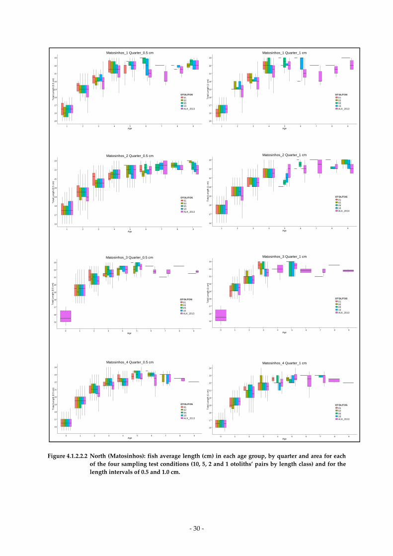
Figure 4.1.2.2.1 shows the boxplots with fish average length in each age group, by area for each of the four sampling test conditions (10, 5, 2 and 1 pairs of otoliths by length class) and the length intervals of 0.5 and 1.0 cm.

- 27 -

Figures 4.1.2.2.2 to 4.1.2.2.4 show the boxplots with fish average length in each age group, by quarter and area for each of the four sampling test conditions (10, 5, 2 and 1 pairs of otoliths by length class) and the length intervals of 0.5 and 1.0 cm.

Figure 4.1.2.2.5 shows the fishing sites geographic positions in the North area from which samples were used for comparing the mean length at age group from samples from different vessels fishing in different areas.

Figure 4.1.2.2.6 presents the Tukey HSD test results comparing the mean length of the samples collected from catches undertaken in the sites/quarters shown in figure 4.1.2.2.5.

Table 4.1.2.2.1 Mean length (cm), standard deviation, number of otoliths and length range in each age group

in the whole year in each area for 10, 5, 2 and 1 otoliths’ pairs by length class and length class intervals of 0.5 and 1.0 cm. These variables are also shown for original ALK’s as a reference (yellow columns). (ALK’s were built based on 0.5 cm length class intervals).

Total_2013_OTOLITOS

Age 0 Age 1 Age 2 Age 3 Age 4 Age 5

0.5 cm 1 cm ALK_2013 0.5 cm 1 cm ALK_2013 0.5 cm 1 cm ALK_2013 0.5 cm 1 cm ALK_2013 0.5 cm 1 cm ALK_2013 0.5 cm

10 OTO Mean Lt(cm) 15.1 15.2 15.6 18.4 18.3 18.6 19.8 19.8 19.6 20.3 20.3 20.4 21.3 21.2 21.0 21.3

s.d. 1.64 1.59 1.61 1.51 1.51 1.41 1.24 1.24 1.29 1.31 1.33 1.23 1.02 1.07 1.05 1.09

nº otoliths 278 141 447 1298 678 1967 1089 528 2182 849 432 1618 471 249 998 288

LT(cm) min 10.5 11.0 10.5 13.0 13.0 13.0 15.5 16.2 15.5 16.5 17.0 16.5 18.0 18.0 17.2 18.6

LT(cm) max 18.8 18.4 19.7 22.9 22.3 22.9 23.2 23.2 23.2 24.3 24.3 24.3 23.6 23.4 24.0 24.3

5 OTO Mean Lt(cm) 15.2 15.4 15.6 18.3 18.3 18.6 19.8 19.8 19.6 20.3 20.4 20.4 21.3 21.3 21.0 21.5

s.d. 1.71 1.66 1.61 1.53 1.55 1.41 1.30 1.30 1.29 1.38 1.37 1.23 1.01 1.16 1.05 1.14

nº otoliths 171 82 447 751 382 1967 619 299 2182 481 245 1618 255 143 998 169

LT(cm) min 10.5 11.0 10.5 13.0 13.0 13.0 15.5 16.2 15.5 16.5 17.0 16.5 18.2 18.0 17.2 18.6

LT(cm) max 18.3 18.4 19.7 22.9 22.3 22.9 23.2 22.3 23.2 24.3 24.3 24.3 23.6 23.4 24.0 24.3

2 OTO Mean Lt(cm) 15.2 15.3 15.6 18.1 18.2 18.6 19.7 19.6 19.6 20.4 20.4 20.4 21.3 21.5 21.0 21.7

s.d. 1.87 1.72 1.61 1.53 1.67 1.41 1.34 1.31 1.29 1.47 1.41 1.23 1.08 1.06 1.05 1.18

nº otoliths 87 41 447 328 180 1967 265 133 2182 201 90 1618 120 56 998 72

LT(cm) min 10.5 11.0 10.5 13.0 13.0 13.0 15.5 16.2 15.5 17.1 17.3 16.5 18.0 18.3 17.2 19.5

LT(cm) max 18.3 18.3 19.7 22.3 22.1 22.9 23.2 22.3 23.2 24.3 24.3 24.3 23.6 23.2 24.0 24.3

1 OTO Mean Lt(cm) 15.4 15.3 15.6 18.1 17.9 18.6 19.7 19.6 19.6 20.3 20.5 20.4 21.4 21.5 21.0 21.9

s.d. 1.92 1.79 1.61 1.65 1.59 1.41 1.46 1.35 1.29 1.43 1.50 1.23 1.13 1.08 1.05 1.16

nº otoliths 52 25 447 181 88 1967 127 65 2182 105 66 1618 64 30 9 98 49

LT(cm) min 10.6 11.0 10.5 13.0 13.0 13.0 15.5 16.2 15.5 17.3 17.1 16.5 18.0 20.0 17.2 19.7

LT(cm) max 18.4 18.2 19.7 21.5 20.3 22.9 22.6 22.3 23.2 24.3 24.3 24.3 23.6 23.4 24.0 24.3

Matosinhos_2013_OTOLITOS



10 OTO Mean Lt(cm) 16.7 16.8 16.4 19.0 18.9 19.1 20.3 20.3 20.0 21.1 21.1 21.0 21.8 21.7 21.7 22.2

s.d. 0.63 0.68 0.88 1.39 1.42 1.26 1.17 1.17 1.36 1.06 1.09 1.09 0.81 0.85 0.90 1.04

nº otoliths 72 39 132 501 256 879 427 203 812 239 117 524 199 104 277 62

LT(cm) min 15.5 16.0 14.5 15.3 15.3 15.3 17.0 17.0 16.0 17.8 19.0 16.5 19.4 19.4 18.3 18.6

LT(cm) max 18.4 18.4 19.3 22.9 22.3 22.9 23.2 23.2 23.2 24.3 24.3 24.3 23.6 23.4 23.8 23.9

5 OTO Mean Lt(cm) 16.7 16.9 16.4 18.9 18.9 19.1 20.3 20.2 20.0 21.1 21.2 21.0 21.9 21.9 21.7 22.3

s.d. 0.66 0.72 0.88 1.43 1.49 1.26 1.19 1.23 1.36 1.14 1.17 1.09 0.77 0.88 0.90 1.04

nº otoliths 47 25 132 276 140 879 224 112 812 138 66 524 107 56 277 38.00

LT(cm) min 15.5 16.0 14.5 15.3 15.3 15.3 17.1 17.0 16.0 17.8 19.0 16.5 20.2 19.4 18.3 18.6

LT(cm) max 18.3 18.4 19.3 22.9 22.3 22.9 23.2 22.3 23.2 24.3 24.3 24.3 23.6 23.4 23.8 23.9

2 OTO Mean Lt(cm) 16.7 16.9 16.4 18.9 18.9 19.1 20.3 20.2 20.0 21.1 21.2 21.0 21.9 21.9 21.7 22.3

s.d. 0.66 0.72 0.88 1.43 1.49 1.26 1.19 1.23 1.36 1.14 1.17 1.09 0.77 0.88 0.90 1.04

nº otoliths 47 25 132 276 140 879 224 112 812 138 66 524 107 56 277 38

LT(cm) min 15.5 16.0 14.5 15.3 15.3 15.3 17.1 17.0 16.0 17.8 19.0 16.5 20.2 19.4 18.3 18.6

LT(cm) max 18.3 18.4 19.3 22.9 22.3 22.9 23.2 22.3 23.2 24.3 24.3 24.3 23.6 23.4 23.8 23.9

1 OTO Mean Lt(cm) 17.0 16.7 16.4 18.9 18.6 19.1 20.4 20.2 20.0 21.2 21.7 21.0 22.0 22.2 21.7 22.4

s.d. 0.78 0.65 0.88 1.44 1.34 1.26 1.23 1.21 1.36 1.19 1.18 1.09 0.94 0.86 0.90 1.07

nº otoliths 13 6 132 58 28 879 49 25 812 27 18 524 23 10 277 12

LT(cm) min 15.9 16.0 14.5 15.4 15.3 15.3 17.3 17.3 16.0 18.7 20.0 16.5 20.2 21.0 18.3 19.7

LT(cm) max 18.4 17.4 19.3 21.5 20.3 22.9 22.6 22.3 23.2 24.3 24.3 24.3 23.6 23.4 23.8 23.9

- 28 -

Table 4.1.2.2.1 Mean length (cm), standard deviation, number of otoliths and length range in each age group in the whole year in each area for 10, 5, 2 and 1 otoliths’ pairs by length class and length class intervals of 0.5 and 1.0 cm. These variables are also shown for original ALK’s as a reference (yellow columns). (ALK’s were built based on 0.5 cm length class intervals). (continued)

Peniche_2013_OTOLITOS



10 OTO Mean Lt(cm) 14.3 14.4 15.2 18.9 18.9 18.9 20.2 20.2 19.9 20.9 20.9 20.7 21.3 21.5 21.3 21.8

s.d. 1.58 1.47 1.85 1.14 1.15 1.13 1.08 1.07 1.07 1.00 1.03 0.98 0.84 0.85 0.82 0.84

nº otoliths 141 70 244 390 201 602 381 184 782 306 164 629 172 83 373 106

LT(cm) min 10.5 11.0 10.5 13.0 13.0 13.0 16.5 17.0 16.5 18.0 18.0 17.7 19.5 20.0 18.7 19.9

LT(cm) max 18.8 18.2 19.7 21.2 21.2 21.3 22.8 22.4 22.8 23.3 23.3 23.3 23.3 23.3 24.0 19.9

5 OTO Mean Lt(cm) 14.3 14.5 15.2 18.8 18.8 18.9 20.2 20.1 19.9 20.9 20.9 20.7 21.4 21.5 21.3 22.1

s.d. 1.71 1.57 1.85 1.17 1.22 1.13 1.15 1.13 1.07 1.11 1.08 0.98 0.86 0.87 0.82 0.83

nº otoliths 84 40 244 241 119 602 223 106 782 161 90 629 88 49 373 57

LT(cm) min 10.5 11.0 10.5 13.0 13.0 13.0 16.5 17.0 16.5 18.0 18.4 17.7 19.7 20.1 18.7 20.3

LT(cm) max 18.2 18.2 19.7 21.1 21.1 21.3 22.6 22.3 22.8 23.3 23.3 23.3 23.3 23.1 24.0 24.3

2 OTO Mean Lt(cm) 14.6 14.8 15.2 18.6 18.7 18.9 20.1 20.0 19.9 21.1 20.9 20.7 21.4 21.7 21.3 22.3

s.d. 1.96 1.76 1.85 1.20 1.39 1.13 1.16 1.19 1.07 1.08 1.12 0.98 0.98 0.81 0.82 0.99

nº otoliths 45 23 244 108 61 602 96 46 782 67 26 629 44 24 373 27

LT(cm) min 10.5 11.0 10.5 13.0 13.0 13.0 16.8 17.2 16.5 18.4 19.3 17.7 19.5 20.2 18.7 20.0

LT(cm) max 18.2 18.2 19.7 21.0 21.1 21.3 22.3 22.3 22.8 23.3 23.1 23.3 23.3 23.1 24.0 24.3

1 OTO Mean Lt(cm) 14.8 15.1 15.2 18.5 18.3 18.9 20.1 20.1 19.9 20.8 20.8 20.7 21.5 21.5 21.3 22.5

s.d. 2.08 1.91 1.85 1.46 1.51 1.13 1.38 1.12 1.07 1.11 1.14 0.98 0.93 1.09 0.82 1.01

nº otoliths 26 15 244 64 31 602 40 18 782 37 25 629 26 13 373 17

LT(cm) min 10.6 11.0 10.5 13.0 13.0 13.0 17.0 18.3 16.5 18.8 18.3 17.7 19.7 20.1 18.7 20.3

LT(cm) max 18.2 18.2 19.7 21.0 20.3 21.3 22.6 22.3 22.8 23.3 23.1 23.3 23.1 23.3 24.0 24.3

Portimao_2013_OTOLITOS



10 OTO Mean Lt(cm) 15.1 15.1 15.3 17.1 17.2 17.3 18.7 18.7 18.6 19.2 19.1 19.3 20.1 20.1 20.2 20.5

s.d. 1.09 1.03 1.16 1.19 1.17 1.20 0.80 0.83 0.93 0.89 0.93 0.91 0.73 0.78 0.77 0.63

nº otoliths 65 32 71 407 221 486 281 141 588 304 151 455 100 62 348 120

LT(cm) min 12.2 12.2 12.2 14.3 14.3 14.3 15.5 16.2 15.5 16.5 17 16.5 18 18 17.2 19.2

LT(cm) max 17.6 17.1 17.6 20.3 20.3 20.3 20.8 20.4 21.7 21.4 21.4 21.6 21.6 21.4 22.1 22.5

5 OTO Mean Lt(cm) 15.1 15.1 15.3 17.1 17.0 17.3 18.7 18.6 18.6 19.2 19.3 19.3 20.3 20.0 20.2 20.6

s.d. 1.27 1.19 1.16 1.22 1.14 1.20 0.85 0.88 0.93 0.97 0.97 0.91 0.72 0.92 0.77 0.69

nº otoliths 40 17 71 234 123 486 172 81 588 182 89 455 60 38 348 74

LT(cm) min 12.2 12.2 12.2 14.3 14.3 14.3 15.5 16.2 15.5 16.5 17 16.5 18.2 18 17.2 19.2

LT(cm) max 17.6 17.1 17.6 20.3 20.3 20.3 20.6 20.4 21.7 21.4 21.3 21.6 21.6 21.4 22.1 22.5

2 OTO Mean Lt(cm) 14.8 15.0 15.3 17.0 16.9 17.3 18.6 18.6 18.6 19.1 19.3 19.3 20.3 20.0 20.2 20.9

s.d. 1.39 1.49 1.16 1.26 1.18 1.20 0.91 0.98 0.93 0.96 0.91 0.91 0.83 0.79 0.77 0.77

nº otoliths 20 8 71 114 57 486 71 39 588 76 39 455 29 11 348 33

LT(cm) min 12.2 12.2 12.2 14.3 14.3 14.3 15.5 16.2 15.5 17.1 17.3 16.5 18 18.3 17.2 19.5

LT(cm) max 17.1 17.1 17.6 20.3 19.3 20.3 20.6 20.4 21.7 21.3 21.1 21.6 21.6 21.1 22.1 22.5

1 OTO Mean Lt(cm) 15.0 14.4 15.3 16.9 16.7 17.3 18.5 18.5 18.6 19.1 19.2 19.3 20.3 20.5 20.2 21.0

s.d. 1.56 1.69 1.16 1.31 1.24 1.20 0.96 0.96 0.93 0.97 1.08 0.91 0.98 0.40 0.77 0.77

nº otoliths 13 4 71 59 29 486 38 22 588 41 23 455 15 7 348 20

LT(cm) min 12.2 12.2 12.2 14.3 14.3 14.3 15.5 16.2 15.5 17.3 17.1 16.5 18 20 17.2 20

LT(cm) max 17.1 16.2 17.6 20.3 20.3 20.3 19.7 20.1 21.7 21.3 21.4 21.6 21.5 21.1 22.1 22.5

- 29 -

Figure 4.1.2.2.1 Fish average length (cm) in each age group, for the whole year and by area for each of the four

sampling test conditions (10, 5, 2 and 1 otoliths’ pairs by length class) and the length intervals of 0.5 and 1.0 cm.

- 30 -

Figure 4.1.2.2.2 North (Matosinhos): fish average length (cm) in each age group, by quarter and area for each

of the four sampling test conditions (10, 5, 2 and 1 otoliths’ pairs by length class) and for the length intervals of 0.5 and 1.0 cm.

15

16

17

18

19

20

21

22

23

1 2 3 4 5 6 7 8 9Age

To

tal L

eng

th (

0.5

cm

)

OTOLITOS01020510ALK_2013

Matosinhos_1 Quarter_0.5 cm

15

16

17

18

19

20

21

22

23

1 2 3 4 5 6 7 8 9Age

Tot

al L

en

gth

(1 c

m)


Matosinhos_1 Quarter_1 cm

16

17

18

19

20

21

22

23

1 2 3 4 5 6 7 8 9Age

To

tal L

eng

th (

0.5

cm

)



16

17

18

19

20

21

22

23

1 2 3 4 5 6 7 8 9Age

Tot

al L

en

gth

(1 c

m)



15

16

17

18

19

20

21

22

23

0 1 2 3 4 5 6 7 8 9Age

Tot

al L

en

gth

(0.

5 c

m)



15

16

17

18

19

20

21

22

23

0 1 2 3 4 5 6 7 8 9Age

To

tal L

en

gth

(1

cm

)



16

17

18

19

20

21

22

23

24

0 1 2 3 4 5 6 7 8 9Age

Tot

al L

en

gth

(0.

5 c

m)



16

17

18

19

20

21

22

23

24

0 1 2 3 4 5 6 7 8 9Age

To

tal L

en

gth

(1

cm

)



- 31 -

Figure 4.1.2.2.3 Centre (Peniche): fish average length (cm) in each age group, by quarter and area for each of

the four sampling test conditions (10, 5, 2 and 1 otoliths’ pairs by length class) and the length intervals of 0.5 and 1.0 cm.

13

14

15

16

17

18

19

20

21

22

23

24

1 2 3 4 5 6 7 8 9Age

Tot

al L

engt

h (0

.5 c

m)


Peniche_1 Quarter_0.5 cm

13

14

15

16

17

18

19

20

21

22

23

24

1 2 3 4 5 6 7 8 9Age

Tot

al L

engt

h (1

cm

)


Peniche_1 Quarter_1 cm

16

17

18

19

20

21

22

23

1 2 3 4 5 6 7 8 9Age

Tot

al L

engt

h (0

.5 c

m)



16

17

18

19

20

21

22

23

1 2 3 4 5 6 7 8 9Age

Tot

al L

engt

h (1

cm

)



17

18

19

20

21

22

23

24

0 1 2 3 4 5 6 7 8Age

Tot

al L

engt

h (0

.5 c

m)



17

18

19

20

21

22

23

24

0 1 2 3 4 5 6 7 8Age

Tot

al L

engt

h (1

cm

)



10

11

12

13

14

15

16

17

18

19

20

21

22

23

24

0 1 2 3 4 5 6 7 8Age

Tot

al L

engt

h (0

.5 c

m)



10

11

12

13

14

15

16

17

18

19

20

21

22

23

24

0 1 2 3 4 5 6 7 8Age

Tot

al L

engt

h (1

cm

)



- 32 -

Figure 4.1.2.2.4 South (Portimão): fish average length (cm) in each age group, by quarter and area for each of

the four sampling test conditions (10, 5, 2 and 1 otoliths’ pairs by length class) and the length intervals of 0.5 and 1.0 cm.

14

15

16

17

18

19

20

21

22

1 2 3 4 5 6 7 8 9Age

To

tal L

engt

h (0

.5 c

m)


Portimao_1 Quarter_0.5 cm

14

15

16

17

18

19

20

21

22

1 2 3 4 5 6 7 8 9Age

Tot

al L

eng

th (1

cm

)


Portimao_1 Quarter_1 cm

15

16

17

18

19

20

21

22

23

1 2 3 4 5 6 7 8 9Age

To

tal L

engt

h (0

.5 c

m)



15

16

17

18

19

20

21

22

23

1 2 3 4 5 6 7 8 9Age

Tot

al L

eng

th (1

cm

)



12

13

14

15

16

17

18

19

20

21

0 1 2 3 4 5 6 7Age

Tot

al L

eng

th (

0.5

cm

)



12

13

14

15

16

17

18

19

20

21

0 1 2 3 4 5 6 7Age

Tot

al L

eng

th (1

cm

)



15

16

17

18

19

20

21

22

0 1 2 3 4 5 6 7 8Age

Tot

al L

eng

th (

0.5

cm

)



15

16

17

18

19

20

21

22

0 1 2 3 4 5 6 7 8Age

Tot

al L

eng

th (1

cm

)



- 33 -

Figure 4.1.2.2.5 Fishing sites in the North area (Q3_C and Q4_A sites are overlapped).

Figure 4.1.2.2.6 Tukey HSD test comparison between mean length by age group from each fishing site and quarters 3 and 4 (see Figure 4.1.2.2.5).

- 34 -

4.4.4.4.2222 Maturity ogivesMaturity ogivesMaturity ogivesMaturity ogives

4.4.4.4.2222.1 Introduction to hake case.1 Introduction to hake case.1 Introduction to hake case.1 Introduction to hake case----studystudystudystudy

The presentation from Costa et al. (P12 – Annex 4) raised several issues related to sampling and estimation of the maturity ogive (MO) for hake (Merluccius merluccius). The main questions raised were related to the time of sampling and the source of hake samples, given the sampling constraints because the species shows a sexual dimorphism in terms of growth and maturation (sex-ratio is 1:1 till ~ 35 cm of length, whereas at bigger sizes females are predominant in relation to males), and likely also presents ontogenetic and sexual changes in spatial distributions. However, MOs in assessment are sex combined.

Pros and cons of current sampling concerning the time of the year and the source of sampling off the Portuguese coast are (Costa et al., P12 – Annex4):

- If samples are taken during Autumn IBTS demersal surveys, the main advantage is that a larger range of sizes is sampled and proportions of mature fish at length can be more accurately raised to the abundances estimated during the surveys. The disadvantages are: the survey takes place out of the main spawning season, there is an increased probability of macroscopic misidentification of immature/resting individuals (no histological validation).

- If samples are taken from commercial catches: it is difficult to obtain non eviscerated fish, smaller individuals (<27 cm) are unavailable (with the consequent limitations for the logistic model fitting), the size distribution of the fish landed depends on the gear used (different selectivity between polyvalent and bottom trawl). The main advantage is that it is possible to obtain samples during the main spawning season. However, are the market samples representatives of the population? Can the spatial distribution of males and females and the proportion of mature fish be inferred without bias from market samples?

4.4.4.4.2222.2 Improving the estimation of maturity ogive.2 Improving the estimation of maturity ogive.2 Improving the estimation of maturity ogive.2 Improving the estimation of maturity ogive

Following the discussions on this subject during the workshop additional analyses were carried out in order to clarify the effect of the timing and source of sampling, and to identify the potential sources of bias in the estimation of the MOs, namely:

- Analyse the sex-ratio distribution along the coast for the demersal research surveys (PNAB): Autumn 2004.

- Use the data from microscopic gonad stage classification to obtain a proportion of immature/resting to apply to MO.

Preliminary results showed that sex ratio is similar along the coast, with a slight increase in the offshore stations (Figure 4.2.2.1).

The length-at-first maturity, L50 (estimated from the fitting of the MO) does not differ when using macroscopic data from samples collected during the 2007 Winter demersal survey (March), during the main spawning season (L50=28.73 cm), or the ones from market, collected in the same season (L50=28.80 cm) (Figure 4.2.2.2).

The use of data from histological gonad stage classification to obtain a proportion of immature/resting to apply to MO also gives close values of L50 (L50=31.75 cm) when compared with the same data from macroscopic identification (L50=32.92 cm) (Figure 4.2.2.3).

The MOs estimated from the 2004 Autumn and the 2005 Winter surveys revealed slight differences in L50 (Figure 4.2.2.4).

- 35 -

The analysis of the MOs estimated with a 1:1 proportion of males and females vs the real observed sex ratio shows that the L50 is slightly higher when the proportion 1:1 of both sexes is considered (Figure 4.2.2.5).

Figure 4.2.2.1 Sex ratio by (a) region and (b) near the coast vs off-shore from the 2004 Winter demersal survey.

Figure 4.2.2.2 Maturity ogives (macroscopic staging) from samples collected during the Winter demersal survey (left panel) and from the market sampling in Feb-Apr (right panel), in year 2007.

(a) (b)

- 36 -

Figure 4.2.2.3 Maturity ogives estimated with GLM fit based on macroscopic (left panel) and histological staging (right panel).

Figure 4.2.2.4 Maturity ogive (macroscopic staging) estimated with GLM from (a) 2004 Autumn survey and (b) 2005 Winter survey.

(a) (b)

- 37 -

Figure 4.2.2.5 Maturity ogives (macroscopic staging) considering (a) all data and (b) a 1:1 sex-ratio based on samples collected during the 2004 Autumn survey.

4.4.4.4.3333 Discussion and ConclusionsDiscussion and ConclusionsDiscussion and ConclusionsDiscussion and Conclusions

4.3.1 Growth4.3.1 Growth4.3.1 Growth4.3.1 Growth

The analyses of the sardine case-study (Section 4.1.2) indicate that there will be no significant differences in the length distribution by age-group if the number of otoliths selected in each length class is reduced. At the age group composition and length distribution the results obtained reducing to 5 the otoliths selected by length class were similar to what is the present situation, considering the ALK’s only regarding 2013. The reduced number of samples usually collected from age group 6+, may explain bigger differences found in average length at age observed in older age groups in the different tests undertaken.

The analysis of the number of otoliths by sample in each area and quarter pointed out that satisfactory results can be achieved with 5 or even 2 otoliths by length class.

From the quarter analyses, a 1.0 cm length class interval option is not advisable due to a higher variability observed. However, when considering the total by year and area the results assuming 1.0 cm length class interval do not show so obvious differences in comparison to 0.5 cm length class interval.

Sardine case-study was a first approach to the Portuguese species sampling design optimization for age data collection to estimate age-length keys. The mean length by age group varies among areas (Soares, P11 Annex 4) despite sardine being caught mostly with one “fishing-gear” (purse-seine). A comparison of the mean length from samples collected in the North area, by port and month, was performed. Despite the very low number of samples, there are significant differences in combinations of sites/quarters (Figure 4.1.2.2.6), which suggest that the samples selection must consider these factors. This analysis should be performed for other areas and years to confirm the observed variability before any change to the current otoliths sampling design.

The analysis performed for sardine should be extended to other species and should include factors like “fishing gear”, “fishing site stratum” (depth), “landing harbour” which may be particularly important for species with wider distribution and caught by several fleet segments. The effects of using a stratified design by port and quarter (or other variables) should be accounted for in the estimation of the final age-length keys for the overall Portuguese landings. The possibility of taking

- 38 -

advantage of probability-based market sampling to obtain probability-based age sampling may be considered in the future as a means to obtain a more design-based sampling scheme.

4.3.2 Reproduction4.3.2 Reproduction4.3.2 Reproduction4.3.2 Reproduction

The analysis of the hake case-study (Section 4.2) indicated that sex and maturity data from the Autumn demersal surveys could be used to predict the maturity ogive (MO) of the following year. This approach should be further explored given the absence of demersal surveys during the peak of hake spawning season (January-March) and market sampling constraints (hake is landed gutted). Therefore, it is recommended to perform a comparison between the macroscopic maturity data from the 2011 Autumn demersal survey and the 2012 macroscopic and microscopic maturity data from market samples during the spawning season. However, it is emphasized that predicting MO requires additional assumptions, namely on growth and mortality rates during the period between the Autumn demersal survey and the spawning season in the following year. Hence, it is highly recommended to estimate MO from in-year market samples.

The sampling design should be based on the analysis of available data from port sampling, in particular to: investigate the distribution of lengths/sexes/mature fish per gear and fishing area to better characterize the spatial distribution of mature fish. It was also suggested that efforts be doubled to obtain representative samples from the fleet, randomizing the sampled trips. Additionally, samples of smaller fish (< 27 cm, not landed) could be obtained from onboard sampled trips. It is noted that the upcoming "landing obligation" may allow these specimens to be sampled on-shore.

Further, bottom-trawl stations conducted during the triennial horse-mackerel DEPM (daily egg production method) surveys, carried out in January-February, might be explored to collect additional data on hake maturity.

5555 RecommendationsRecommendationsRecommendationsRecommendations and Future Workand Future Workand Future Workand Future Work

ToR 1)

- Randomization of landing events within sampling days should be improved.

- Extend the feasibility evaluation of combining concurrent sampling and species-focus sampling to the analysis of precision of the mean length estimates.

- Explore other sampling strategies (e.g., sampling directly for size categories instead of sampling trips) and ponder the development of a pilot study including field experiments.

- Compare the different raising methods (e.g., current, design-based, by categories), particularly in relation to the updated design where the SSU are trips.

The following recommendations to improve fishery data are addressed to DGRM and DOCAPESCA:

- At the landing port several species need to be correctly identified and discriminated at species level.

- Include in the daily landing database of SLV (Serviços de Lota e Vendagem, DOCAPESCA) the discrimination of the fishing gear(s) used at the trip level.

- 39 -

ToR 2)

Sampling onboard long-distance longline fleet operating in the Indian Ocean:

- If only one observer can be allocated to the onboard sampling programme, it is recommended a switch between fishing areas (West and East), starting with the area with less coverage.

Sampling onboard vessels in Division IXa:

- Collect information on refusal rates by fleet segment.

- Investigate the existence of reference fleets for segments where random sampling is not possible due to high refusal rates.

The following recommendations are addressed to DGRM and SWWAC:

- Facilitate updated list of contacts of masters and skippers and indicate the type of information skippers /masters /associations would like to receive from PNAB-IPMA onboard sampling programme.

ToR 3)

- The approach used in the sardine case-study to optimize the sampling design for age data collection should be applied to other species.

- The sardine analysis suggested a significant reduction on the number of otoliths required to estimate the ALK´s used in the stock assessment. However, additional analyses should be performed before any change to the current sampling design.

- Following the analyses and discussions on hake reproduction and maturity ogives, it is suggested to explore the use of the microscopic gonad stage classification to estimate the proportion of immature/resting in the length range where macroscopic staging can be misidentified.

- Analyse the available data from port sampling to investigate the distribution of lengths/sexes/mature fish per gear and fishing area to better characterize the spatial distribution of mature fish and base the maturity market/onboard sampling design.

- Explore the effects of different raising procedures on ALK´s and maturity ogive estimates.

Imprecise and biased stock assessment input data, like those analysed and discussed in the workshop, strongly affect the quality of key parameter estimates, like fishing mortality (F) and spawning stock biomass (SSB). A framework for cost-efficient sampling to support stock assessment was presented by Vølstad (Vølstad et al, P09 – Annex 4). An Open Source software (StoX) currently under development at IMR will support reproducible stock assessments, where estimates of parameters such as spawning stock (biomass and numbers) and fishing mortality (F) can be presented with associated measures of precision (e.g., relative standard errors or confidence intervals). In particular, the StoX programs will allow the quantification of the propagation of sampling errors in input data obtained from catch-sampling surveys and scientific trawl surveys (i.e., fishery dependent or independent data) to the stock assessment results used in quota advice. The tool will include methods for quantifying sampling errors in swept-area estimates and acoustic estimates of numbers-at-age and numbers-at-length using data, based on methods in Aanes and Vølstad (in review) and Stenevik et al. (2014), as well as sampling errors in estimates of catch in numbers-at-age or numbers-at-length from catch sampling surveys, using the model ECA (Hirst et al. 2012).

- 40 -

6666 ReferencesReferencesReferencesReferences

Aanes, S. and J.H. Vølstad. In Review. Efficient statistical estimators and sampling strategies for estimating the age-composition of fish. Can. J. Fish. Aquat. Sci.

EC (2001). Commission Regulation (EC) No. 1639/2001 establishing the minimum and extended Community programmes for the collection of data in the fisheries sector and laying down detailed rules for the application of Council Regulation (EC) No. 1543/2000.

EC (2009). EU Commission Decision (2010/93/EU) of 18 December 2009, adopting a multiannual Community programme for the collection, management and use of data in the fisheries sector for the period 2011-2013 (notified under document C(2009) 10121.

Hirst, D., G. Storvik, H. Rognebakke, S. Aanes and J. H. Vølstad (2012). A modeling approach to the estimation of catch-at-age of commercial fish species. Canadian Journal of Fisheries and Aquatic Sciences 69: 1–13. doi:10.1139/CJFAS-2012-0075.

Murawski, S. A., S. E. Wigley, M. J. Fogarty, P.J. Rago, and D. G. Mountain (2005). Effort distribution and catch patterns adjacent to temperate MPAs. ICES Journal of Marine Science, 62: 1150-1167.

Rago, P. J., S. E. Wigley and M. J. Fogarty (2005). NEFSC bycatch estimation methodology: allocation, precision, and accuracy. U.S. Dep. Commer., Northeast Fish. Sci. Cent. Ref. Doc. 05-09, 44 p. Available from: National Marine Fisheries Service, 166 Water Street, Woods Hole, MA 2543-1026.

Stenevik, E.K., J.H. Vølstad, Å Høines, S. Aanes, G.J. Óskarsson, J.A. Jacobsen and Ø. Tangen (2014). Precision in estimates of density and biomass of Norwegian spring spawning herring based on acoustic surveys. Mar.Biol. Res. (In press)

Sullivan, P. J., F. J. Breidt, R. B. Ditton, B. A. Knuth, B. M. Leaman, V. M. O’Connell, G. R. Parsons, K. H. Pollock, and S.L. Stokes (2006). Review of recreational fisheries survey methods. Ocean Studies Board–Division on Earth and Life Studies, National Research Council of the National Academies, Washington, DC, 187p.

Vølstad, J. H. and M. Fogarty (2006). Report on the National Observer Program Vessel Selection Bias Workshop. Woods Hole, May 17-19, 2006. 532 pp.

- 41 -

Annex 1: List of participantsAnnex 1: List of participantsAnnex 1: List of participantsAnnex 1: List of participants

List of participants:

Ricardo Alpoim

IPMA - Algés

[email protected]

Ana Cláudia Fernandes

IPMA- Algés

[email protected]

João Pereira

IPMA- Algés

[email protected]

Manuela Azevedo (chair)

IPMA- Algés

[email protected]

Ivone Figueiredo

IPMA- Algés

[email protected]

Nuno Prista

IPMA- Algés

[email protected]

Corina Chaves

IPMA- Algés

[email protected]

Patricia Gonçalves

IPMA- Algés

[email protected]

Cristina Silva (chair)

IPMA- Algés

[email protected]

Ana Maria Costa

IPMA- Algés

[email protected]

Pedro Lino

IPMA-Olhão

[email protected]

Eduardo Soares

IPMA- Algés

[email protected]

Marina Dias

IPMA- Algés

[email protected]

Ana Moreno

IPMA- Algés

[email protected]

Jorge Vargas

IPMA- Algés

[email protected]

Sandra Dores

IPMA- Algés

[email protected]

Teresa Moura

IPMA- Algés

[email protected]

Jon H. Vølstad (chair)

IMR – Bergen

[email protected]

Mónica Felício

IPMA-Matosinhos

mfelí[email protected]

Cristina Nunes

IPMA- Algés

[email protected]

- 42 -

List of invited participants:

Paula Abreu

IPMA - Algés

[email protected]

Susana Godinho

DGRM

[email protected]

Daniel Pinto

IPMA- Algés

[email protected]

António Fernandes

IPMA- Algés

[email protected]

Elizabete Henriques

IPMA- Algés

[email protected]

Sílvia Lourenço

IPMA- Algés

slourenç[email protected]

Ana Luísa Ferreira

IPMA- Algés

[email protected]

Mónica Inácio

IPMA- Algés

[email protected]

Carmo Silva

IPMA- Algés

[email protected]

Maria João Ferreira

IPMA- Algés

[email protected]

Hugo Mendes

IPMA-Algés

[email protected]

Dina Silva

IPMA-Algés

[email protected]

Teresa Fonseca

SWWAC

[email protected]

- 43 -

Annex 2: Meeting Agenda Annex 2: Meeting Agenda Annex 2: Meeting Agenda Annex 2: Meeting Agenda

WORKSHOP ON SAMPLING DESIGN AND OPTIMIZATION (WKSDO)

IPMA, 17 – 20 November 2014 (4 days)

Objectives:

- Analysis of current sampling designs and their optimization: • market sampling for length composition • onboard sampling for catches • sampling for biological parameters

Agenda

Day 1

09:00 – 09:30 Startup procedures. Presentation of participants.

Workshop TORs

Introductory presentation: Portuguese fleets and fisheries – M. Azevedo, C. Silva, M. Dias

09:30 – 10:30 TOR 1: Market sampling design to estimate the length composition of landings. Concurrent sampling and species focus sampling.

Presentations:

- Present sampling design (10+5 min) – N. Prista, M. Dias - Rays (10+5 min) – I. Figueiredo, C. Maia - Anglerfishes (10+5 min) – R. Alpoim, T. Moura, N. Prista

10:30 – 10:50 Coffee break

10:50 – 12:30 Presentations:

- Catch length composition estimated from commercial size-categories: does it improve accuracy? – M. Azevedo, C. Silva

- Sampling designs – J. H. Vølstad

Discussion:

Market sampling design, sampling effort and precision.

Approaches and definition of case studies to be discussed in working groups.

12:30 – 14:00 Lunch

14:00 – 16:00 Working groups


16:20 – 17:30 Presentation of WGs results. Summary of the discussions.

- 44 -

Day 2

09:00 – 10:30 TOR 2: Catch sampling onboard

Presentations:

- Sampling design in Div. IXa (10+5 min) – A. C. Fernandes, N. Prista - Sampling design in Indian Ocean (10+5 min) – P. G. Lino, R. Coelho, M. N.

Santos

Discussion:

Objectives, sampling design, sampling effort, constraints, raising, how to improve the precision of estimates.


10:50 – 12:30 Discussion (continuation)

12:30 – 14:00 Lunch

14:00 – 16:00 Presentation:

- Framework for assessing monitoring effort to support stock assessment - J. H. Vølstad

Working groups


16:20 – 17:30 Summary of the discussions.

Day 3

09:00 – 10:30 TOR 3: Biological sampling

Presentations:

- Sampling/precision ALKs – J. H. Vølstad - Sampling for age / ALKs, CS Sardine (10+5 min) – E. Soares - Sampling for maturity / maturity ogive, CS Hake (10+5 min) – A. M. Costa,

C. Nunes, J. Pereira


10:50 – 12:30 Discussion

12:30 – 14:00 Lunch

14:00 – 17:30 Working groups and summary of discussions

Day 4




12:30 – 14:00 Lunch

14:00 – 17:30 Report writing (Discussion and Conclusions). End

- 45 -

Annex 3: Glossary of statistical terms Annex 3: Glossary of statistical terms Annex 3: Glossary of statistical terms Annex 3: Glossary of statistical terms

Statistics POPULATION (População): complete set of items from which we may collect data.

TARGET POPULATION (População alvo): is the entire group about which the researcher wishes to draw conclusions.

STUDY POPULATION (População de estudo): is the group from which sample is to be drawn.

SAMPLE (Amostra): is a group of units selected from a larger group (the population). By studying the sample one expects to draw valid conclusions about the larger group.

SAMPLING UNIT1 (Unidade de amostragem): In order to take a sample from a population, the population must consist of, or be divided into non-overlapping parts (units). Sampling can then be conducted by selecting units according to a defined sampling scheme. The units that can be selected in catch sampling schemes are typically groups, e.g. the group of fish landed from a fishing trip or group of fish caught in a fishing operation.

PRIMARY SAMPLING UNIT1 (Unidade de amostragem primária): A sampling unit in the first stage in a multi-stage sampling scheme is called a primary sampling unit. Examples of primary sampling units in the most common catch sampling schemes are trips, vessels, landing places or site-days.

NON-PROBABILITY SAMPLING (Amostragem não-probabilística): sampling units are selected deliberately (based on attributes), because they are convenient (easily accessed) or haphazardly (one cannot guarantee that the sampling units are selected independently of their measurement values). An example of non-probability sampling is quota sampling.

PROBABILITY SAMPLING (Amostragem probabilística): sampling units are selected so that every sampling unit has non-zero probability of being present in the sample and no unit is guaranteed to be selected (execpt in very unusual instances), Sampling strategies for probability sampling include simple random, stratified, systematic or cluster.

SAMPLING FRAME1 (Lista de amostragem): In statistics, a sampling frame is the list of sampling units or device from which a sample can be drawn. The sampling frame comprises all the sampling units and any stratification of these, and may be based, e.g., on a vessel registry or list of ports.

SAMPLING DESIGN (Desenho amostral): The set of rules that govern the sampling.

SAMPLING STRATEGIES (Estratégias de amostragem): there are several methods for selecting a sample:

RANDOM SAMPLING (Amostragem aleatória) – Each individual is chosen entirely by chance and each element of the population has a known, but possibly non-equal, chance of being included in the sample.

SIMPLE RANDOM SAMPLING (Amostragem aleatória simples) 3 – each individual is chosen entirely by chance and each element of the population has the same probability of being selected. There are two ways of selecting a simple random sample, with replacement or without replacement of the sampling units selected.

UNEQUAL PROBABILITY RANDOM SAMPLING (Amostragem aleatória com probabilidades desiguais) – each individual is chosen entirely by chance and but elements of the population have different probabilities of being selected. There are two ways of selecting a simple random sample, with replacement or without replacement of the sampling units selected.

- 46 -

STRATIFIED SAMPLING (Amostragem estratificada) – the whole population is divided into non-overlapping subpopulations, called strata (singular: stratum), from which samples are taken. Stratification can used be to achieve designated precision levels at stratum level, for convenience of implementation and/or to obtain overall gains in precision of final population-level estimates. In general, gains in precision are obtained when strata are internally homogeneous/similar but heterogenous/dissimilar between each other. Samples can be selected from each stratum using random sampling (with or without replacement) or unequal probability sampling.

CLUSTER SAMPLING (Amostragem por conglomerados) 3 – the whole population is partitioned into groups called clusters, each containing one or more elements, but the sampling units are the clusters. As opposed to the strata, the clusters are preferably based on heterogeneity/dissimilarity within cluster and homogeneity/similarity among clusters. Clusters may be selected using, e.g., simple random sampling. In some books cluster sampling is considered to include multistage sampling-

MULTISTAGE SAMPLING(Amostragem multietápica) 3 – several sampling methods are combined into successive sampling stages. At each stage, there is probability-based selection of sampling units, which can be clusters (initial phase) or elements (final stage)or clusters. Stratification can also be used in multistage sampling. In some books multistage sampling is included in cluster sampling.

SYSTEMATIC SAMPLING (Amostragem sequencial)3 – The population elements are ordered and a first element is randomly selected. Subsequent elements are selected every kth element from the starting point.

QUOTA SAMPLING (Amostragem por quotas) – Sampling is carried out from a random starting element until a pre-defined quota is attained (the designated sampling effort). This strategy suffers from a number of methodological flaws, the most basic of which is that the sample is not a random sample and therefore the sampling distributions of any statistics are unknown.

STRATIFICATION1 (Estratificação): The advance decomposition of a finite population of sampling

units of size N into k non-overlapping subpopulations (strata) of size iN .

POST-STRATIFICATION or STRATIFICATION AFTER SELECTION1 (Pós-estratificação): If a simple random sample is taken from a finite population of sampling units of size N the sample may

be treated as a stratified sample during the analysis if the post-strata sizes iN are know. Stratification

after selection (post-stratification) is usually applied if the strata to which the selected sampling units belong are only known after the sample is taken or one is interested in estimates for different subpopulations than the originally envisioned. This is often the case for métiers. Standard stratified estimators may have to be weighed when a métier crosses sampling strata.

SAMPLING EFFORT (Esforço de amostragem): Number of samples to collect. Sampling effort can be optimized to achieve the precision levels required for a certain estimate, taking into account the costs of sampling and the variance of the samples/strata.

ACCURACY (Exactidão): an indicator of the closeness of an estimated value (e.g. population parameter) to the actual value.

PRECISION4 (Precisão): is a measure of how close an estimator is expected to be to the true value of a parameter. Precision is usually expressed in terms of imprecision and related to the standard error of the estimator. Less precision is reflected by a larger standard error (or a larger coefficient of variation).

- 47 -

BIAS4 (Enviesamento): a term which refers to how far the average statistic lies from the parameter it is estimating, that is, the error which arises when estimating a quantity. Errors from chance will cancel each other out in the long run, those from bias will not.

Low precision High precision

Lower accuracy

(low bias)

Higher accuracy

(high bias)

Fisheries section

CONCURRENT SAMPLING2 (Amostragem simultânea): Sampling all or a predefined group of species that are simultaneously present in landings (or catches) of a certain fishing trip.

FLEET1 (Frota): A physical group of vessels sharing similar characteristics in terms of technical features and/or major activity.

FISHERY1 (Pescaria): A group of trips targeting the same species assemblage and/or stocks, using similar gear, during the same period of the year and within the same area.

FLEET SEGMENT2 (Segmento de frota): A group of vessels with the same length class (LOA) and predominant fishing gear during the year, e.g. according to the Appendix III of the EU-DCF. Vessels may have different fishing activities during the reference period, but are classified in only one fleet segment.

MÉTIER1,2: A group of fishing operations targeting a similar (assemblage of) species, using similar gear, during the same period of the year and/or within the same area and which are characterised by a similar exploitation pattern.

HIERARCHICAL LIST OF SPECIES2 (Lista hierárquica de espécies): When there is no possibility to do the “concurrent sampling”, a list of species with major interest is needed. This list must include species of relevance for management purposes and for which a request is made by an international scientific body or a regional fisheries management organisation (DCF). It can be compiled in accordance to DCF requisites (combination of species groups and sampling schemes adopted).

1 ICES. 2012. Report of the second Workshop on Practical Implementation of Statistical Sound Catch Sampling Programs, 6 - 9 November 2012, ICES Copenhagen. ICES CM 2012 / ACOM: 52, 71p

2 EU Commission Decision (2010/93/EU) of 18 December 2009, adopting a multiannual Community programme for the collection, management and use of data in the fisheries sector for the period 2011-2013 (notified under document C(2009)

10121)

3 Cadima, E.L.; Caramelo, A.M.; Afonso-Dias, M; Conte de Barros, P.; Tandstad, M.O.; de Leiva Moreno, J.I.. 2005. Sampling methods applied to fishing science: a manual. FAO Fisheries Technical Paper. No. 434. Rome, FAO. 88p.

4 Statistics Glossary (STEPS internet site)

- 48 -

Annex 4: PresentationsAnnex 4: PresentationsAnnex 4: PresentationsAnnex 4: Presentations

P01P01P01P01

- 49 -

- 50 -

P02P02P02P02

- 51 -

- 52 -

P03P03P03P03

- 53 -

- 54 -

- 55 -

P04P04P04P04

- 56 -

- 57 -

P05P05P05P05

- 58 -

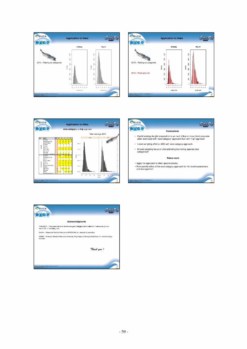
- 59 -

- 60 -

P06P06P06P06

- 61 -

- 62 -

- 63 -

- 64 -

- 65 -

P07P07P07P07

- 66 -

- 67 -

P08P08P08P08

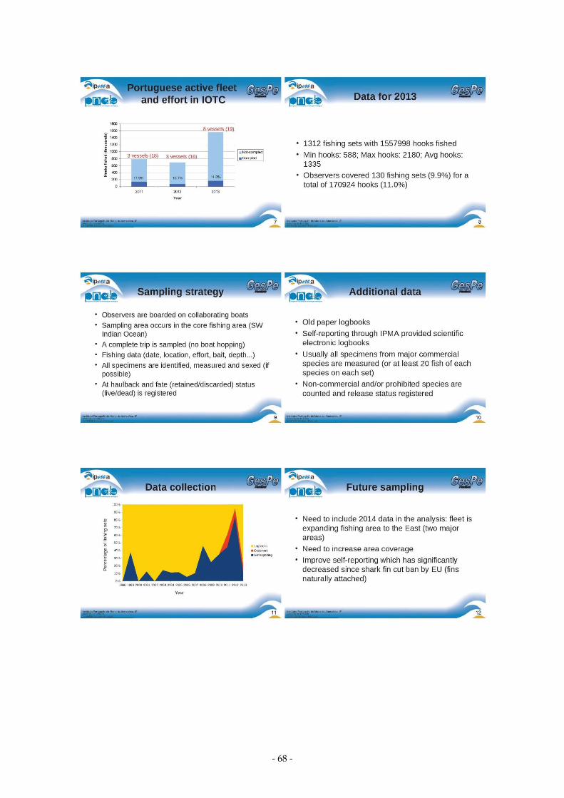
- 68 -

- 69 -

P09P09P09P09

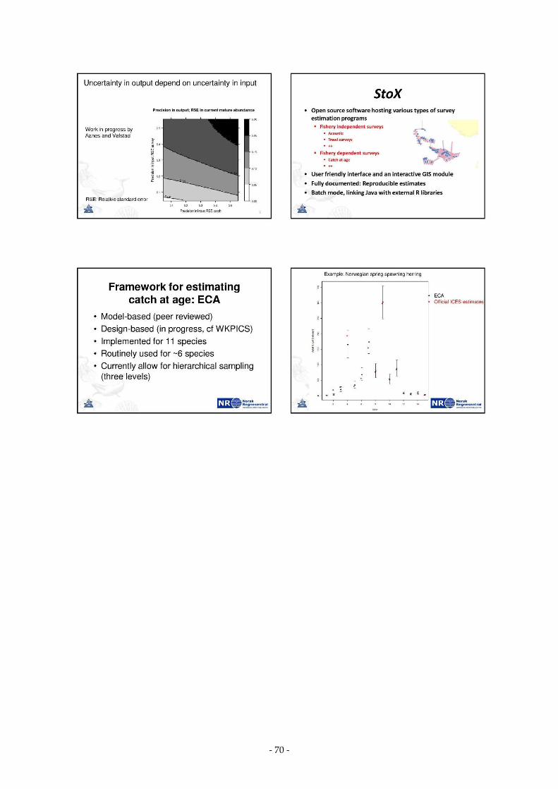
- 70 -

- 71 -

P10P10P10P10

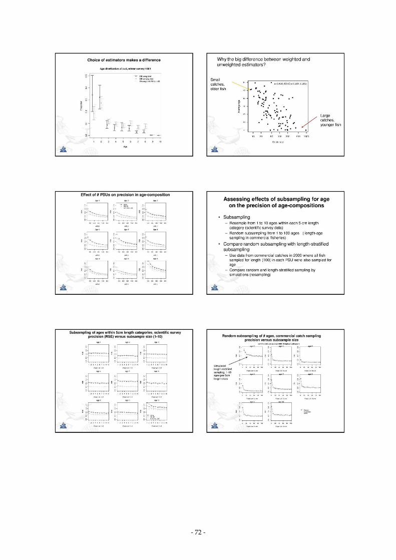
- 72 -

- 73 -

- 74 -

- 75 -

P11P11P11P11

- 76 -

- 77 -

- 78 -

P12P12P12P12

- 79 -

- 80 -

MINISTÉRIO DA AGRICULTURA, E DO MAR

relatórios científicos e técnicos ipma, série digital, 2

Documents