quantum properties of a non-abelian gauge invariant action with a mass parameter

Quantum properties of a non-Abelian gauge invariant action with a mass parameter

M. A. L. Capri,1,* D. Dudal,2,† J. A. Gracey,3,‡ V. E. R. Lemes,1,x R. F. Sobreiro,1,k S. P. Sorella,1,{ and H. Verschelde2,**1UERJ - Universidade do Estado do Rio de Janeiro, Rua Sao Francisco Xavier 524, 20550-013 Maracana, Rio de Janeiro, Brasil

2Ghent University, Department of Mathematical Physics and Astronomy, Krijgslaan 281-S9B-9000 Gent, Belgium3Theoretical Physics Division Department of Mathematical Sciences, University of Liverpool,

P.O. Box 147, Liverpool, L69 3BX, United Kingdom(Received 14 June 2006; published 11 August 2006)

We continue the study of a local, gauge invariant Yang-Mills action containing a mass parameter, whichwe constructed in a previous paper starting from the nonlocal gauge invariant mass dimension twooperator F��D2��1F��. We return briefly to the renormalizability of the model, which can be proven toall orders of perturbation theory by embedding it in a more general model with a larger symmetry content.We point out the existence of a nilpotent Becchi-Rouet-Stora-Tyutin (BRST) symmetry. Although ouraction contains extra (anti)commuting tensor fields and coupling constants, we prove that our model in thelimit of vanishing mass is equivalent with ordinary massless Yang-Mills theories. The full theory isrenormalized explicitly at two loops in the MS scheme and all the renormalization group functions arepresented. We end with some comments on the potential relevance of this gauge model for the issue of adynamical gluon mass generation.

DOI: 10.1103/PhysRevD.74.045008 PACS numbers: 11.15.�q, 11.10.Gh

I. INTRODUCTION

Yang-Mills gauge theories, with quantum chromody-namics (QCD) modeling the strong interaction betweenelementary particles as one of the key examples, are quitewell understood at very high energies. In this energyregion, asymptotic freedom [1–4] sets in, which in turnensures that the coupling constant g2 is small enough tomake a perturbative expansion in powers of g2 possible.The elementary QCD excitations are the gluons andquarks.

Our current understanding of non-Abelian gauge theo-ries is still incomplete in the infrared region. At lowerenergies, the interaction grows stronger, preventing theuse of standard perturbation theory to obtain relativelyacceptable results. Nonperturbative aspects of the theorycome into play. The most notable, yet to be rigorouslyproven nonperturbative phenomenon, is the fact that theelementary gluon and quark excitations no longer belongto the physical spectrum, being confined into colorlessstates such as glueballs, mesons, and baryons.

A widely used strategy to parametrize certain nonper-turbative effects of the theory amounts to the introductionof so-called condensates, which are the expectation valuesof certain operators in the vacuum. Furthermore, one canemploy the operator product expansion (OPE) (viz. shortdistance expansion) which can be applied to local opera-tors, in order to relate the associated condensates to non-

perturbative power corrections which, in turn, giveadditional information next to the perturbatively calculablecontributions.

As we are considering a gauge theory, these condensatesshould be gauge invariant if they are to enter physicalobservables. This puts rather strong restrictions on thepossible condensates, the ones with lowest dimensionalityare the dimension three quark condensate h � i and thedimension four gluon condensate hF2

��i. There is a varietyof methods to obtain estimates of these condensates, suchas the phenomological approach based on the Shifman-Vainshtein-Zakharov (SVZ) sum rules, [5] for a recentoverview, the use of lattice methods [6], as well as theuse of instanton calculus [7].

Gauge condensates are necessarily nonperturbative innature, as gauge theories do not contain a mass term in theaction due to the requirement of gauge invariance.However, through nonperturbative effects, a nontrivialvalue for e.g. hF2

��i can arise.In [8], it was already argued that also gauge variant

condensates could influence gauge variant quantities suchas the gluon propagator. In particular, the dimension twogluon condensate hA2

�i has received much attention in theLandau gauge [9–34] over the past few years. An OPEargument based on lattice simulations has provided evi-dence that this condensate could account for quadraticpower corrections of the form� 1

Q2 , reported in the running

of the coupling constant as well as in the gluon propagator[11,13,14,24,27,31,33].

This nonvanishing condensate hA2�i gives rise to a dy-

namically generated gluon mass [11,12,16,19,20]. Theappearance of mass parameters in the gluon two pointfunction is a common feature of the expressions employedto fit the numerical data obtained from lattice simulations

*Electronic address: [email protected]†Electronic address: [email protected]‡Electronic address: [email protected] address: [email protected] address: [email protected]{Electronic address: [email protected]

**Electronic address: [email protected]

PHYSICAL REVIEW D 74, 045008 (2006)

1550-7998=2006=74(4)=045008(14) 045008-1 © 2006 The American Physical Society

http://dx.doi.org/10.1103/PhysRevD.74.045008

[35–37]. Let us mention that a gluon mass has been foundto be useful also in the phenomenological context [38,39].

The local operator A2� in the Landau gauge has wit-

nessed a renewed interest due to the recent works [9,10],as the quantity

hA2mini � min

U2SU�N�

1

VT

Zd4xh�AU��

2i; (1)

which is gauge invariant due to the minimization along thegauge orbits, could be physically relevant. In fact, as shownin [9,10] in the case of compact three-dimensional QED,the quantity hA2

mini seems to be useful in order to detect thepresence of nontrivial field configurations like monopoles.One should notice that the operator A2

min is highly nonlocaland therefore it falls beyond the standard OPE realm thatrefers to local operators. One can show that A2

min can bewritten as an infinite series of nonlocal terms, see [40,41]and references therein, namely

A2min �

1

2

Zd4x

�Aa�

��

@�@�@2

�Aa�

� gfabc�@�@2 @A

a��

1

@2 @Ab�Ac�

��O�A4�: (2)

However, in the Landau gauge, @�A� � 0, all nonlocalterms of expression (2) drop out, so that A2

min reduces to thelocal operator A2

�, hence the interest in the Landau gaugeand its dimension two gluon condensate. However, a com-plication, as already outlined in our previous paper [40], isthat the explicit determination of the absolute minimum ofA2� along its gauge orbit, and moreover of its vacuum

expectation value, is a very delicate issue intimately relatedto the problem of the Gribov copies [42]. We refer to [40]for some more explanation and the original referencesconcerning this point.

Nevertheless, some nontrivial results were proven con-cerning the operator A2

�. In particular, we mention itsmultiplicative renormalizability to all orders of perturba-tion theory, in addition to an interesting and numericallyverified relation concerning its anomalous dimension[15,43]. An effective potential approach consistent withthe renormalization group requirements has also beenworked out for this operator, giving further evidence of anonvanishing condensate hA2

�i � 0, which lowers the non-perturbative vacuum energy [12].

A somewhat weak point about the operator A2min is that it

is unclear how to deal with it in gauges other than theLandau gauge. Until now, it seems hopeless to prove itsrenormalizability out of the Landau gauge. In fact, at theclassical level, adding (1) to the Yang-Mills action isequivalent to adding the so-called Stueckelberg action,which is known to be not renormalizable [44,45]. We refer,once more, to [40] for details and references.

In recent years, some progress has also been made in thepotential relevance of dimension two condensates beyond

the Landau gauge. We were able to prove the renormaliz-ability of certain local operators like: A2

� in the linearcovariant gauges, ( 1

2Aa�Aa� � � �caca) in the nonlinear

Curci-Ferrari gauges, and ( 12A

��A

�� c�c�) in the maxi-

mal Abelian gauges [46]. A renormalizable effective po-tential for these operators has been constructed, giving riseto a nontrivial value for the corresponding condensates,and a dynamical gluon mass parameter emerged in each ofthese gauges [47–51]. There also have been attempts toinclude possible effects of Gribov copies [18,21,52,53].Unfortunately, the amount of numerical data availablefrom lattice simulations is rather scarce in the aforemen-tioned gauges. Nevertheless, let us mention that a dynami-cal gluon mass in the maximal Abelian gauge has beenreported in [54,55]. In the Coulomb gauge too, the rele-vance of a dimension two condensate has been touchedupon in the past [56].

Although the renormalizability of the foregoing dimen-sion two operators is a nontrivial and important fact in itsown right, their lack of gauge invariance is a less welcomefeature. Moreover, at present, it is yet an open questionwhether these operators might be related in some way to agauge invariant gluon mass.

Many aspects of the dimension two condensates and ofthe related issue of dynamical mass generation in Yang-Mills theories need further understanding. An importantstep forward would be a gauge invariant mechanism be-hind a dynamical mass, without giving up the importantrenormalization aspects of quantum field theory.

We set a first step in this direction in our previous paper[40]. As a local gauge invariant operator of dimension twodoes not exist, and since locality of the action is almostindispensable to prove renormalizability to all orders andto have a consistent calculational framework at hand, wecould look for a nonlocal operator that is localizable byintroducing an additional set of fields. As pointed out in[40], this task looks extremely difficult for the operatorA2

min if we reckon that an infinite series of nonlocal terms isrequired, as displayed in (2). Instead, we turned our atten-tion to the gauge invariant operator

F1

D2 F �1

VT

Zd4xFa��D2��1abFb��; (3)

where D2 � D�D� is the covariant Laplacian, D� beingthe adjoint covariant derivative. The operator (3) alreadyappeared in relation to gluon mass generation in three-dimensional Yang-Mills theories [57].

The usefulness of the operator (3) relies on the fact that,when it is added to the usual Yang-Mills Lagrangian bymeans of � 1

4m2F 1

D2 F, the resulting action can be easilycast into a local form by introducing a finite set of auxiliaryfields [40]. Starting from that particular localized action,we succeeded in constructing a gauge invariant classicalaction Scl containing the mass parameter m, enjoyingrenormalizability. This action Scl was identified to be

M. A. L. CAPRI et al. PHYSICAL REVIEW D 74, 045008 (2006)

045008-2

Sphys � Scl � Sgf; (4)

Scl�Zd4x

�1

4Fa��F

a��

im4�B� �B�a��F

a��

�1

4� �Ba��Dab

� Dbc� Bc�� Ga

��Dab� Dbc

� Gc��

�3

8m2�1� �Ba��B

a�� Ga

��Ga��m

2�3

32� �Ba��B

a��

2

��abcd

16� �Ba��Bb�� Ga

��Gb�� Bc��Bd�� Gc

��Gd��

�;

(5)

Sgf �Zd4x

��2baba � ba@�Aa� � �ca@�Dab

� cb�: (6)

We notice that we had to introduce a new quartic tensorcoupling �abcd, as well as two new mass couplings �1 and�3. The renormalizability was proven to all orders in theclass of linear covariant gauges, implemented through Sgf,via the algebraic renormalization formalism [58]. Withoutthe new couplings, i.e. when �1 � 0, �3 � 0, �abcd � 0,the previous action would not be renormalizable.

In this paper, we present further results concerning theaction (5) obtained in [40]. In Sec. II, we provide a shortsummary of the construction of the model (5) and wepresent a detailed discussion of the renormalization ofthe tensor coupling �abcd, not given in [40]. We drawattention to the existence of an extended version of theusual nilpotent BRST symmetry for the model (4). Weintroduce a kind of supersymmetry between the novelfields fBa��, �Ba��, Ga

��, �Ga��g which is enjoyed by the

massless version, m � 0, of the action (4). In Sec. III, wediscuss the explicit renormalization of several quantities.The fields and the mass m are renormalized to two looporder in the MS scheme. The �abcd-function of the tensorcoupling �abcd is determined at one loop, by means ofwhich it shall also become clear that radiative corrections(re)introduce anyhow the quartic interaction in the novelfields in the action (4). These fields are thus more thansimple auxiliary fields, which appear at most quadratically.A few internal checks on the results are included, such asthe explicit gauge parameter independence of the anoma-lous dimension ofm. It is also found that the original Yang-Mills quantities renormalize identically as when the usualYang-Mills action would have been used. This is indicativeof the fact that the massless version of (4) might beequivalent to Yang-Mills theory, quantized in the samegauge. This is a nontrivial statement, due to the presenceof the term proportional to the tensor coupling �abcd. InSec. IV, we use the aforementioned supersymmetry toactually prove the equivalence between the massless ver-sion of (4) and Yang-Mills theories. In the concludingSec. V, we put forward a few suggestions that might beuseful for future research directions.

II. SURVEY OF THE CONSTRUCTION OF THEMODEL AND ITS RENORMALIZABILITY

In this section we present a short summary of how wecame to the construction of our model (4) in [40]. We shallalso point out a few properties of the corresponding actionnot explicitly mentioned in [40].

A. The model at the classical level

We start from the Yang-Mills action SYM supplementedwith a gauge invariant although nonlocal mass operator

SYM � SO; (7)

with the usual Yang-Mills action defined by

SYM �1

4

Zd4xFa��F

a��; (8)

and with

SO � �m2

4

Zd4xFa��D2��1abFb��: (9)

The field strength is given by

Fa�� @�Aa� � @�A

a� � gf

abcAb�Ac�; (10)

and the adjoint covariant derivative by

Dab� � @��ab � gfabcAc�: (11)

In order to have a consistent calculational framework at theperturbative level, we need a local action. To our knowl-edge, it is unknown how to treat an action like (7), such asproving its renormalizability to all orders of perturbationtheory. This is due to the presence of the nonlocal term (9).As we have discussed in [40], the action (7) can be local-ized by introducing a pair of complex bosonic antisym-metric tensor fields, (Ba��, �Ba��), and a pair of complexanticommuting antisymmetric tensor fields, ( �Ga

��, Ga��),

belonging to the adjoint representation, according to which

e�SO �ZD �BDBD �GDG exp

��

�1

4

Zd4x �Ba��Dab

� Dbc� Bc��

�1

4

Zd4x �Ga

��Dab� D

bc� G

c��

�im4

Zd4x�B� �B�a��F

a��

��: (12)

It is worth mentioning the special limit m � 0, in whichcase we have in fact introduced nothing more than a rathercomplicated unity written as [59] ZD �BDBD �GDG exp

��

�1

4

Zd4x �Ba��Dab

� Dbc� Bc��

�1

4

Zd4x �Ga

��Dab� D

bc� G

c��

�� 1: (13)

Hence, we have obtained a local, classical, and gaugeinvariant action

QUANTUM PROPERTIES OF A NON-ABELIAN GAUGE . . . PHYSICAL REVIEW D 74, 045008 (2006)

045008-3

S � SYM � SBG � Sm; (14)

where

SBG �1

4

Zd4x� �Ba��D

ab� D

bc� B

c�� Ga

��Dab� D

bc� G

c��;

Sm �im4

Zd4x�B� �B�a��F

a��: (15)

The gauge transformations are given by

�Aa� � �Dab� !

b; �Ba�� gfabc!bBc��;

� �Ba�� gfabc!b �Bc��; �Ga�� gfabc!bGc

��;

� �Ga�� gfabc!b �Gc

��;

(16)

with !a parametrizing an arbitrary infinitesimal gaugetransformation, so that

�S � ��SYM � SBG � Sm� � 0: (17)

B. The model at the quantum level

Evidently, the construction of the classical action (14) isonly a first step. We still need to investigate if this actioncan be renormalized when the quantum corrections areincluded. This highly nontrivial task was treated at lengthin [40] to which we refer the interested reader for back-ground information. Nevertheless, we shall take some timeto explain the main idea as well as to present a detailedanalysis of the quantum corrections affecting the quartictensor coupling �abcd.

As the quantization of a locally invariant gauge modelrequires the fixing of the gauge freedom, we shall employthe linear covariant gauge fixing from now on, as it wasdone in [40], and which is imposed via (6).

To actually discuss the renormalizability of (14), wefound it useful to embed it into a more general class ofmodels described by the action

� � SYM � Sgf �Zd4x� �Bai D

ab� D

bc� B

ci �

�Gai D

ab� D

bc� G

ci �

�Zd4x�� Ui��Ga

i � Vi�� Bai � �Vi��Bai

�Ui��Gai �F

a�� 1� �Vi��@2Vi�� Ui��@2Ui��

�Zd4x2� �Vi��@�@�Vi�� Ui��@�@�Ui��

�Zd4x� �Ui��Ui��

�Uj��Uj��

� �Vi��Vi�� Vj��Vj�� 2 �Ui��Ui��Vj��Vj��; (18)

where use has been made of a composite Lorentz index i ��; ��, i � 1 . . . 6, corresponding to a global U�6� symme-try [40] of the action (18). The quantities Vi��, �Ui��,Ui��,and �Ui�� are local sources. The identification betweenobjects carrying indices i and (�, �) is determined through

�Bai ; �Bai ;Gai ; �Ga

i � �12�B

a��; �Ba��;G

a��; �Ga

��;

�Vi��; �Vi��;Ui��; �Ui�� 12�V��;

�V��;U��; �U��:

(19)

The free parameters 1, 2, and are needed for renorma-lizability purposes. As far as we are considering Greenfunctions of elementary fields, their role is irrelevant asthey multiply terms which are polynomial in the externalsources.

The reason for introducing the action (18) is that form � 0, the action (14) enjoys a few global symmetrieswhich are lost for m � 0, whereas the action (18) alsoenjoys these symmetries when the global symmetry trans-formations are suitably extended to the sources. We refer to[40] for the details. Evidently, the general action (18) mustpossess the action (14) we are interested in as a specialcase. The reader can check that the connection is made byconsidering the ‘‘physical’’ limit

limphys

�V�� limphys

V�� im

2�� ;

limphys

�U�� limphys

U�� 0; (20)

i.e.

limphys

� � S: (21)

In [40], it was shown that the action (18) obeys a large setof Ward identities. We shall not list them here, but mentionthat the action � is invariant under a nilpotent BRSTtransformation s, acting on the fields as

sAa� � �Dab� cb; sca �

g2fabccbcc;

sBa�� gfabccbBc�� Ga��; s �Ba�� gfabccb �Bc��;

sGa�� gfabccbGc

��; s �Ga�� gfabccb �Gc

�� Ba��;

s �ca � ba; sba � 0; (22)

and on the sources as

sVi�� Ui��; sUi�� 0;

s �Ui�� Vi��; s �Vi�� 0;(23)

such that

s� � 0; s2 � 0: (24)

By employing the algebraic renormalization technique[58], it was found that (18) is not yet the most generalaction compatible with all the Ward identities, includingthe Slavnov-Taylor identity associated to the BRST invari-ance described by (24). The most general and renormaliz-able action was identified to be

Sgen � �� S�; (25)

where


045008-4

S� �Zd4x

��1� �Bai B

ai �

�Gai G

ai �� Vj��Vj�� Uj��Uj��

�abcd

16� �Bai B

bi �

�Gai G

bi �� BcjB

dj �

�GcjG

dj �

� �3

��Bai G

ajVi�� Uj�� Ga

i GajUi��

�Uj�� Bai BajVi�� Vj�� Ga

i BajUi��

�Vj�� Gai B

aj

�Ui��Vj��

� �Gai

�BajUi��Vj�� 1

2Bai B

aj

�Vi�� Vj�� 1

2Gai G

aj

�Ui��Uj��

1

2�Bai �BajVi��Vj��

1

2�Gai

�GajUi��Uj��

��: (26)

The quantities �1 and �3 are independent scalar couplings,whereas �abcd is an invariant rank 4 tensor coupling,obeying the generalized Jacobi identity

fman�mbcd � fmbn�amcd � fmcn�abmd � fmdn�abcm � 0;

(27)

and subject to the following symmetry constraints

�abcd � �cdab; �abcd � �bacd; (28)

which can be read off from the vertex that �abcd multiplies.When we specify the action (25) to the physical values(20), we obtain the main outcome of the paper [40], whichis the physical action Sphys given in (4), that is renormaliz-able to all orders of perturbation theory in the linearcovariant gauge, imposed via Sgf. The renormalizabilityis of course ensured as (4) is a special case of the moregeneral renormalizable action (25), since

limphys

Sgen � Sphys: (29)

We notice that the couplings �1 and �3 are in fact part ofthe mass matrix of the fields fBa��, �Ba��, Ga

��, �Ga��g.

We end this subsection by mentioning that the classicalaction Scl is also invariant with respect to the gauge trans-formations (16), since the terms / f�1; �3; �

abcdg are sepa-rately gauge invariant.

C. The renormalization of the tensor coupling �abcd

As already mentioned, this section is devoted to provid-ing further details of the renormalization of the tensorcoupling �abcd, not fully covered in [40].

The term we are interested in at the level of the bare [60]action is given by

Zd4x

��abcdo

16� �Bai;oB

bi;o �

�Gai;oG

bi;o�� Bcj;oB

dj;o �

�Gcj;oG

dj;o�

�;

(30)

where, in the notation of [40]

fB; �B;G; �Ggao;i ��Zb

pfB; �B;G; �Ggai

� �1� ��a3 �12a4�fB; �B;G; �Ggai ; (31)

where a3, a4 are arbitrary coefficients and � stands for aperturbative expansion parameter [40].

The most general counterterm corresponding to therenormalization of the 4-point vertex � �Bai B

bi �

�Gai G

bi �

� �BcjBdj �

�GcjG

dj � turns out to be given by

�4a3 � ~a6�Mabcd

16� �Bai B

bi �

�Gai G

bi �� BcjB

dj �

�GcjG

dj �; (32)

where ~a6 is a free coefficient and Mabcd is an arbitraryinvariant rank 4 tensor, composed of all the other availabletensors (such as �abcd, �ab, fabc and invariant objectsconstructed from these and Ta). By the Ward identities, itis nevertheless restricted by

M abcd �Mcdab; Mabcd �Mbacd; (33)

which are of course the same symmetry constraints asthose for �abcd, see (28). Also the Jacobi identity (27)applies to Mabcd.

The counterterm is thus not necessarily directly propor-tional to the original tensor �abcd. This has a simple dia-grammatical explanation, as diagrams contributing to the4-point interaction / � �Bai B

bi �

�Gai G

bi �� BcjB

dj �

�GcjG

dj � can

be constructed with the other available interactions. Thisalso means that, even if �abcd � 0, radiative correctionsshall reintroduce this 4-point interaction. This shall be-come more clear in Sec. III, where the explicit results arediscussed.

We can thus decompose the bare tensor coupling �abcdoas

�abcdo � Z�abcd � Zabcd; (34)

where Z and Zabcd contain the counterterm information,more precisely Z contains the counterterm informationdirectly proportional to �abcd, while Zabcd contains, so tosay, all the rest. Evidently, Zabcd will obey analogousconstraints as given in (28) or (33). The tensor Mabcd

can be decomposed similarly into

M abcd � �abcd �Mabcd � �abcd|��{z��}�N abcd

: (35)

In the previous paper [40], we erroneously omitted theN abcd part. Using (32), (34), and (35) allows for a simpleidentification, being

Z � 1� ��~a6 � 2a4�; Zabcd � ��4a3 � ~a6�Nabcd:

(36)

Consequently, the model is still renormalizable to all or-ders, although �abcd is not multiplicatively renormalizable


045008-5

in the naive sense. The situation can be directly comparedwith Higgs inspired models like the Coleman-Weinbergaction [61,62], in the sense that also there a similar mixingoccurs between the different couplings, namely of thegauge coupling e2 and the Higgs coupling �. This is nicelyreflected in the �-functions for the couplings, which areseries in both e2 and �. It is even so that setting the Higgscoupling � � 0 does not make ��e2; �� vanish. See [62]for the three loop expressions. As we shall discuss later inthis paper, the �abcd-function of the tensor coupling �abcd

will be influenced by the gauge coupling g2. Vice versa,one might expect that �abcd could enter, in a suitablecolorless combination, the �g2 -function for g2. This ishowever not the case. We shall present the general argu-ment behind this in Sec. IV. The �g2-function remains thusidentical to the well-known ��g2�-function of Yang-Millstheory.

Let us end this subsection by mentioning that the methodof using the extended action (25), which is a generalizationof another action like (4) and which exhibits a larger set ofWard identities, turns out to be a powerful tool in order toestablish renormalizability to all orders. This is reminis-cent of Zwanziger’s approach to prove the renormalizabil-ity of a local action describing the restriction to the firstGribov horizon [63,64].

D. A few words about the BRST symmetry and a kindof supersymmetry

Let us now return for a moment to the action Sphys givenin (4). As it is a gauge fixed action, we expect that it shouldhave a nilpotent BRST symmetry. However, one shalleasily recognize that the BRST transformation s as definedin (22) no longer constitutes a symmetry of the action (4).This is due to the fact that setting the sources to theirphysical values (20) breaks the BRST s as the transforma-tions (23) are incompatible with the desired physical values(20).

Let us take a closer look at the breaking of this BRSTtransformation s. Let us define another transformation ~s atthe level of the fields by

~sAa� � �Dab� cb; ~sca �

g2fabccacb;

~sBa�� gfabccbBc��; ~s �Ba�� gfabccb �Bc��;

~sGa�� gfabccbGc��; ~s �Ga

�� gfabccb �Gc��;

~s �ca � ba; ~sba � 0:

(37)

A little algebra yields

~sSphys � 0; (38)

~s 2 � 0: (39)

Hence, the action S is invariant with respect to a nilpotentBRST transformation ~s. We obtained thus a gauge fieldtheory, described by the action S, (4), containing a massterm, and which has the property of being renormalizable,while nevertheless a nilpotent BRST transformation ex-pressing the gauge invariance after gauge fixing existssimultaneously. It is clear that ~s stands for the usualBRST transformation, well known from literature, on theoriginal Yang-Mills fields, whereas the gauge fixing partSgf given in (6) can be written as a ~s-variation, ensuringthat the gauge invariant physical operators shall not dependon the choice of the gauge parameter [58].

We can relate ~s and s. Let us start from the originallocalized action (14) and let us set m � 0. Then it enjoys anilpotent ‘‘supersymmetry’’ between the auxiliary tensorfields fBa��, �Ba��, Ga

��, �Ga��g, more precisely if we define

the (anticommuting) transformation �s as

�sBa�� Ga��; �sGa

�� 0; �s �Ga�� Ba��;

�s �Ba�� 0; �s� � 0 for all other fields�;(40)

then one can check that

�2s � 0; �s�Sjm�0� � 0: (41)

Let us mention for further use that, �s being a nilpotentoperator, it possesses its own cohomology, which is easilyidentified with polynomials in the original Yang-Millsfields fAa�, ba, ca, �cag. The auxiliary tensor fields, fBa��,�Ba��,Ga

��, �Ga��g, do not belong to the cohomology of �s, as

a consequence of the fact that they form pairs of doublets[58].

Taking a closer look upon Eqs. (22), (37), and (40), oneimmediately verifies that

s � ~s� �s: (42)

When m � 0, the action (14) is no longer �s-invariant.Nevertheless, this �s-symmetry can be kept if the moregeneral action (18) is employed, when we extend the�s-invariance to the introduced sources [65] as

�sVi�� Ui��; �sUi�� 0;

�s �Ui�� Vi��; �s �Vi�� 0:(43)

Eventually, the most general and renormalizable action(25) turns out to be compatible with the �s-invariancetoo, as it should be. This is obvious if we recognize thatwe can write


045008-6

Sgen � SYM � Sgf � �sZd4x �Ga

i Dab� D

bc� B

ci � �s

Zd4x��Vi�� Ga

i � �Ui��Bai �F

a�� 1

�Ui��@2Vi�� 2

�Ui��@�@�Vi��

� � �Ui��Vi�� Vj��Vj�� Ui��Vi�� Uj��Uj�� sZd4x

��1�Bai �Ga

i � �Vj��Vj�� Uj��Uj��

� �abcd�� Bai Bbi �

�Gai G

bi ��

�GcjB

cj�� 3�Baj �Uj�� Bai Vi�� Ga

i Ui�� 12�3�Baj �Uj��Ga

i�Ui�� Bai �Vi��

� 12�3� �Ga

jVj�� Gai Ui�� Bai Vi��

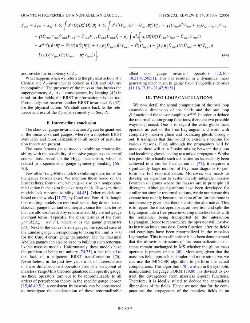
�; (44)

and invoke the nilpotency of �s.What happens when we return to the physical action (4)?

Clearly, the �s-invariance is broken as (20) and (43) areincompatible. The presence of the mass m thus breaks thesupersymmetry �s. As a consequence, by keeping (42) inmind for the fields, the BRST tranformation s is lost too.Fortunately, we recover another BRST invariance ~s, (37),for the physical action. We shall come back to the rele-vance and use of the �s-supersymmetry in Sec. IV.

E. Intermediate conclusion

The classical gauge invariant action Scl can be quantizedin the linear covariant gauges, whereby a nilpotent BRSTsymmetry and renormalizability to all orders of perturba-tion theory are present.

The most famous gauge models exhibiting renormaliz-ability with the possibility of massive gauge bosons are ofcourse those based on the Higgs mechanism, which isrelated to a spontaneous gauge symmetry breaking [66–70].

Few other Yang-Mills models exhibiting mass terms forthe gauge bosons exist. We mention those based on theStueckelberg formalism, which give rise to a nonpolyno-mial action in the extra Stueckelberg fields. However, thesemodels lack renormalizability [44,45]. Other models arebased on the works [71,72] by Curci and Ferrari. Althoughthe resulting models are renormalizable, they do not have aclassical gauge invariant counterpart, since the mass termsthat are allowed/needed by renormalizability are not gaugeinvariant terms. Typically, the mass term is of the form12m

2�Aa�Aa� � � �caca�, where � is the gauge parameter[73]. Next to the Curci-Ferrari gauges, the special case ofthe Landau gauge, corresponding to taking the limit � � 0for the Curci-Ferrari gauge parameter, and the maximalAbelian gauges can also be used to build up such renorma-lizable massive models. Unfortunately, these models havethe problem of being not unitary [74,75], a fact related tothe lack of a nilpotent BRST transformation [76].Nevertheless, in the past few years a lot of interest arosein these dimension two operators from the viewpoint ofmassless Yang-Mills theories quantized in a specific gauge.As these operators turn out to be renormalizable to allorders of perturbation theory in the specific gauge chosen[15,48,49,51], a consistent framework can be constructedto investigate the condensation of these renormalizable

albeit non gauge invariant operators [12,16–18,21,47,50,51]. This has resulted in a dynamical massgenerating mechanism in gauge fixed Yang-Mills theories[11,16,17,19–21,47,50,51].

III. TWO LOOP CALCULATIONS

We now detail the actual computation of the two loopanomalous dimension of the fields and the one loop�-function of the tensor coupling �abcd. In order to deducethe renormalization group functions, there are two possibleways to proceed. One is to regard the extra gluon massoperator as part of the free Lagrangian and work withcompletely massive gluon and localizing ghosts through-out. It transpires that this would be extremely tedious forvarious reasons. First, although the propagators will bemassive there will be a 2-point mixing between the gluonand localizing ghosts leading to a mixed propagator. Whilstit is possible to handle such a situation, as has recently beenachieved in a similar localization in [77], it requires asignificantly large number of Feynman diagrams to per-form the full renormalization. Moreover, one needs todevelop an algorithm to systematically integrate massiveFeynman diagrams where the masses are in principle alldivergent. Although algorithms have been developed forsimilar but simpler renormalizations, we do not pursue thisavenue here mainly because the extra effort for this route isnot necessary given that there is a simpler alternative. Thisis to regard the mass operator as an insertion and split theLagrangian into a free piece involving massless fields withthe remainder being transported to the interactionLagrangian. Hence to renormalize the operator will involveits insertion into a massless Green function, after the fieldsand couplings have been renormalized in the masslessLagrangian. This is possible since it has been demonstratedthat the ultraviolet structure of the renormalization con-stants remain unchanged in MS whether the gluon massoperator is present or not [40]. Moreover, given that themassless field approach is simpler and more attractive, wecan use the MINCER algorithm to perform the actualcomputations. This algorithm [78], written in the symbolicmanipulation language FORM [79,80], is devised to ex-tract the divergences from massless 2-point functions.Therefore, it is ideally suited to deduce the anomalousdimensions of the fields. Hence we note that for the com-putations the propagators of the massless fields in an


045008-7

arbitrary linear covariant gauge are [40]

hAa��p�Ab��p�i � ��ab

p2

�� 1� ��

p�p�p2

�;

hca�p� �cb��p�i ��ab

p2 ; h �p� � ��p�i �6p

p2 ;

hBa��p� �Bb��p�i � ��ab

2p2 �� ;

hGa��p� �Gb

��p�i � ��ab

2p2 �� ;

(45)

where p is the momentum. Using QGRAF, [81], to gen-erate the two loop Feynman diagrams we have firstchecked that the same two loop anomalous dimensionsemerge for the gluon, Faddeev-Popov ghost, and quarksin an arbitrary linear covariant gauge as when the extralocalizing ghosts are absent. This is primarily due to thefact that the 2-point functions of the fields do not involveany extra ghosts except within diagrams. Then they appearwith equal and opposite signs due to the anticommutativityof the Ga

�� ghosts and hence cancel. This observation shallbe given an explicit proof in Sec. IV. We thus note that theexpressions obtained for the renormalization group func-tions are the same as the two loop MS results of[3,4,82,83]. For the localizing ghosts there is the addedfeature that the properties of the �abcd couplings have to beused, as specified in (27) and (28). We have implementedthese properties in a FORM module. However, we note thatin the renormalization of both localizing ghosts, we haveassumed that

�acde�bcde �1

NA�ab�pqrs�pqrs;

�acde�bdce �1

NA�ab�pqrs�prqs;

(46)

which follows from the fact that there is only one rank twoinvariant tensor in a classical Lie group. If this is notsatisfied then one would require a 2-point counterterminvolving the �abcd couplings which was not evident inthe algebraic renormalization technology which estab-lished the renormalizability of the localized operator.Hence, at two loops in MS we find that

�B�a; �� G�a; ��

� �� 3�a��2

4� 2��

61

6

�C2A

�10

3TFNf

�a2 �

1

128NA�abcd�acbd; (47)

where NA is the dimension of the adjoint representation ofthe color group a � g2=�16 2�, and we have also absorbeda factor of 1=�4 � into �abcd here and in later anomalousdimensions. These anomalous dimensions are consistent

with the general observation that these fields must have thesame renormalization constants, in full agreement with theoutput of the Ward identities [40].

In order to verify that (47) is in fact correct, we haverenormalized the 3-point gluon Ba�� vertex. Since the cou-pling constant renormalization is unaffected by the extralocalizing ghosts (and we have checked this explicitly byrenormalizing the gluon quark vertex), then we can checkthat the same gauge parameter independent coupling con-stant renormalization constant emerges from gluon Ba��vertex. Computing the 7 one loop and 166 two loopFeynman diagrams it is reassuring to record that the vertexis finite with the already determined two loop MS field andcoupling constant renormalization constants. Prior to con-sidering the operator itself, we need to determine the oneloop �-function for the �abcd couplings. As this is presentin a quartic interaction it means that to deduce its renor-malization constant, we need to consider a 4-point func-tion. However, in such a situation the MINCER algorithmis not applicable since two external momenta have to benullified and this will lead to spurious infrared infinitieswhich could potentially corrupt the renormalization con-stant. Therefore, for this renormalization only, we haveresorted to using a temporary mass regularization intro-duced into the computation using the algorithm of [84] andimplemented in FORM. Consequently, we find the gaugeparameter independent renormalization

�abcdo � �abcd ��

1

8��abpq�cpdq � �apbq�cdpq

� �apcq�bpdq � �apdq�bpcq� � 6CA�abcda

� 4CAfabpfcdpa2 � 8CAf

adpfbcpa2

� 48dabcdA a2

�1

"; (48)

from both the �abcd �Ba��Bb�� Bc��Bd�� and�abcd �Ba��B

b�� Gc��G

d�� vertices where dabcdA is the totallysymmetric rank four tensor defined by

dabcdA � Tr�TaAT�bA T

cAT

d�A �; (49)

with TaA denoting the group generator in the adjoint repre-sentation [85]. Dimensional regularization in d � 4� 2"dimensions is used throughout this paper. Producing thesame expression for both these 4-point functions, asidefrom the gauge independence, is a strong check on theircorrectness as well as the correct implementation of thegroup theory. Unlike for the gauge coupling and its�-function, the �abcd �-function contains terms also in-volving the gauge coupling g2 at one loop. Hence, to oneloop �abcd� �a; �� is given by


045008-8

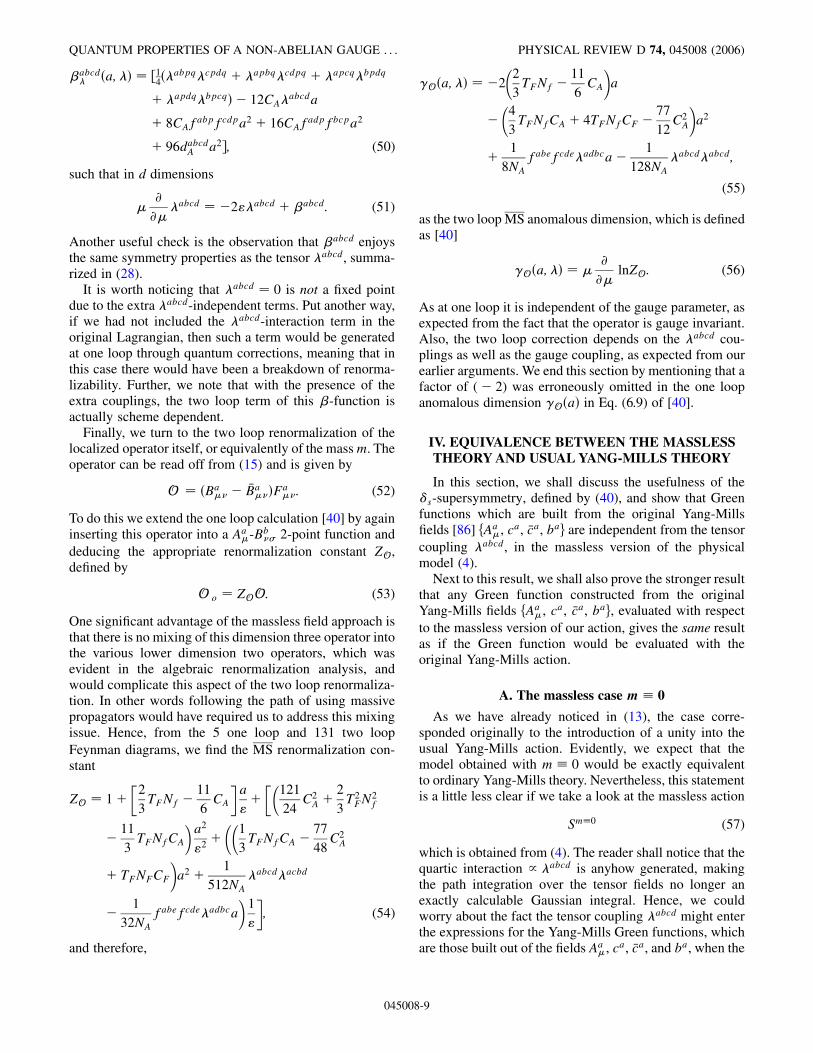
�abcd� �a; �� 14��abpq�cpdq � �apbq�cdpq � �apcq�bpdq

� �apdq�bpcq� � 12CA�abcda

� 8CAfabpfcdpa2 � 16CAfadpfbcpa2

� 96dabcdA a2; (50)

such that in d dimensions

�@@�

�abcd � �2"�abcd � �abcd: (51)

Another useful check is the observation that �abcd enjoysthe same symmetry properties as the tensor �abcd, summa-rized in (28).

It is worth noticing that �abcd � 0 is not a fixed pointdue to the extra �abcd-independent terms. Put another way,if we had not included the �abcd-interaction term in theoriginal Lagrangian, then such a term would be generatedat one loop through quantum corrections, meaning that inthis case there would have been a breakdown of renorma-lizability. Further, we note that with the presence of theextra couplings, the two loop term of this �-function isactually scheme dependent.

Finally, we turn to the two loop renormalization of thelocalized operator itself, or equivalently of the massm. Theoperator can be read off from (15) and is given by

O � �Ba�� Ba��Fa��: (52)

To do this we extend the one loop calculation [40] by againinserting this operator into a Aa�-Bb�� 2-point function anddeducing the appropriate renormalization constant ZO,defined by

O o � ZOO: (53)

One significant advantage of the massless field approach isthat there is no mixing of this dimension three operator intothe various lower dimension two operators, which wasevident in the algebraic renormalization analysis, andwould complicate this aspect of the two loop renormaliza-tion. In other words following the path of using massivepropagators would have required us to address this mixingissue. Hence, from the 5 one loop and 131 two loopFeynman diagrams, we find the MS renormalization con-stant

ZO � 1��

2

3TFNf �

11

6CA

�a"�

��121

24C2A �

2

3T2FN

2f

�11

3TFNfCA

�a2

"2 �

��1

3TFNfCA �

77

48C2A

� TFNFCF

�a2 �

1

512NA�abcd�acbd

�1

32NAfabefcde�adbca

�1

"

�; (54)

and therefore,

�O�a; �� 2�2

3TFNf �

11

6CA

�a

�

�4

3TFNfCA � 4TFNfCF �

77

12C2A

�a2

�1

8NAfabefcde�adbca�

1

128NA�abcd�abcd;

(55)

as the two loop MS anomalous dimension, which is definedas [40]

�O�a; �� @@�

lnZO: (56)

As at one loop it is independent of the gauge parameter, asexpected from the fact that the operator is gauge invariant.Also, the two loop correction depends on the �abcd cou-plings as well as the gauge coupling, as expected from ourearlier arguments. We end this section by mentioning that afactor of (� 2) was erroneously omitted in the one loopanomalous dimension �O�a� in Eq. (6.9) of [40].

IV. EQUIVALENCE BETWEEN THE MASSLESSTHEORY AND USUAL YANG-MILLS THEORY

In this section, we shall discuss the usefulness of the�s-supersymmetry, defined by (40), and show that Greenfunctions which are built from the original Yang-Millsfields [86] fAa�, ca, �ca, bag are independent from the tensorcoupling �abcd, in the massless version of the physicalmodel (4).

Next to this result, we shall also prove the stronger resultthat any Green function constructed from the originalYang-Mills fields fAa�, ca, �ca, bag, evaluated with respectto the massless version of our action, gives the same resultas if the Green function would be evaluated with theoriginal Yang-Mills action.

A. The massless case m � 0

As we have already noticed in (13), the case corre-sponded originally to the introduction of a unity into theusual Yang-Mills action. Evidently, we expect that themodel obtained with m � 0 would be exactly equivalentto ordinary Yang-Mills theory. Nevertheless, this statementis a little less clear if we take a look at the massless action

Sm�0 (57)

which is obtained from (4). The reader shall notice that thequartic interaction / �abcd is anyhow generated, makingthe path integration over the tensor fields no longer anexactly calculable Gaussian integral. Hence, we couldworry about the fact the tensor coupling �abcd might enterthe expressions for the Yang-Mills Green functions, whichare those built out of the fields Aa�, ca, �ca, and ba, when the


045008-9

partition function corresponding to the action (57) wouldbe used.

We recall here that the action (57) is invariant under thesupersymmetry (40). This has its consequences for theGreen functions. Let us explore this now. First, we considera generic n-point function built up only from the originalfields fAa�, ca, �ca, bag. More precisely, we set

G n�x1; . . . ; xn� � hGn�x1; . . . ; xn�iSm�0phys

�ZD�Gn�x1; . . . ; xn�e

�Sm�0phys ; (58)

with

Gn�x1; . . . ; xn� � A�x1� . . .A�xi� �c�xi�1� . . . �c�xj�c�xj�1� . . .

c�xk�b�xk�1� . . . b�xn�; (59)

and we introduced the shorthand notation � denoting allthe fields. We notice that �sGn � 0 whereas Gn � �s�. . .�,i.e. any functional of the form (59) belongs to the�s-cohomology.

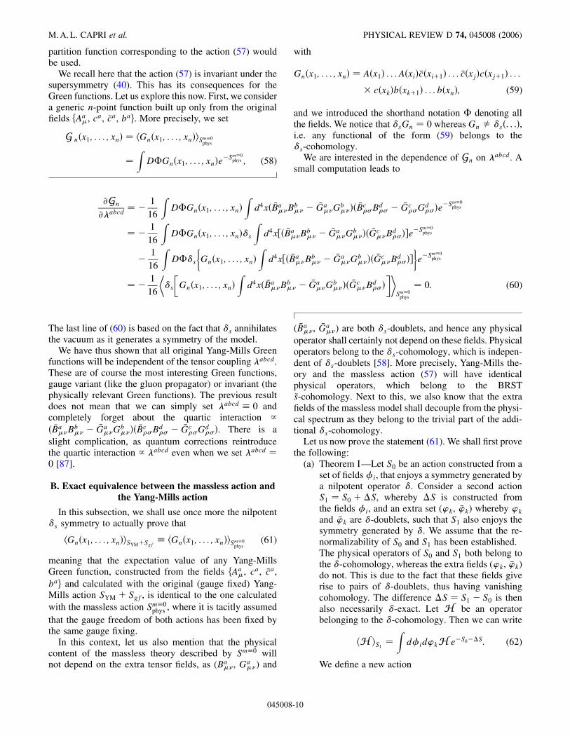
We are interested in the dependence of Gn on �abcd. Asmall computation leads to

@Gn

@�abcd� �

1

16

ZD�Gn�x1; . . . ; xn�

Zd4x� �Ba��Bb�� Ga

��Gb�� Bc��Bd�� Gc

��Gd��e

�Sm�0phys

� �1

16

ZD�Gn�x1; . . . ; xn��s

Zd4x�� Ba��B

b�� Ga

��Gb�� Gc

��Bd��e

�Sm�0phys

�1

16

ZD��s

�Gn�x1; . . . ; xn�

Zd4x�� Ba��B

b�� Ga

��Gb�� Gc

��Bd��

�e�S

m�0phys

� �1

16

�s

�Gn�x1; . . . ; xn�

Zd4x� �Ba��Bb�� Ga

��Gb�� Gc

��Bd��

Sm�0phys

� 0: (60)

The last line of (60) is based on the fact that �s annihilatesthe vacuum as it generates a symmetry of the model.

We have thus shown that all original Yang-Mills Greenfunctions will be independent of the tensor coupling �abcd.These are of course the most interesting Green functions,gauge variant (like the gluon propagator) or invariant (thephysically relevant Green functions). The previous resultdoes not mean that we can simply set �abcd � 0 andcompletely forget about the quartic interaction /

� �Ba��Bb�� Ga��Gb

�� Bc��Bd�� Gc��Gd

��. There is aslight complication, as quantum corrections reintroducethe quartic interaction / �abcd even when we set �abcd �0 [87].

B. Exact equivalence between the massless action andthe Yang-Mills action

In this subsection, we shall use once more the nilpotent�s symmetry to actually prove that

hGn�x1; . . . ; xn�iSYM�Sgf � hGn�x1; . . . ; xn�iSm�0phys

(61)

meaning that the expectation value of any Yang-MillsGreen function, constructed from the fields fAa�, ca, �ca,bag and calculated with the original (gauge fixed) Yang-Mills action SYM � Sgf, is identical to the one calculatedwith the massless action Sm�0

phys , where it is tacitly assumedthat the gauge freedom of both actions has been fixed bythe same gauge fixing.

In this context, let us also mention that the physicalcontent of the massless theory described by Sm�0 willnot depend on the extra tensor fields, as (Ba��, Ga

��) and

( �Ba��, �Ga��) are both �s-doublets, and hence any physical

operator shall certainly not depend on these fields. Physicaloperators belong to the �s-cohomology, which is indepen-dent of �s-doublets [58]. More precisely, Yang-Mills the-ory and the massless action (57) will have identicalphysical operators, which belong to the BRST~s-cohomology. Next to this, we also know that the extrafields of the massless model shall decouple from the physi-cal spectrum as they belong to the trivial part of the addi-tional �s-cohomology.

Let us now prove the statement (61). We shall first provethe following:

(a) Theorem I—Let S0 be an action constructed from aset of fields�i, that enjoys a symmetry generated bya nilpotent operator �. Consider a second actionS1 � S0 ��S, whereby �S is constructed fromthe fields �i, and an extra set (’k, �’k) whereby ’kand �’k are �-doublets, such that S1 also enjoys thesymmetry generated by �. We assume that the re-normalizability of S0 and S1 has been established.The physical operators of S0 and S1 both belong tothe �-cohomology, whereas the extra fields (’k, �’k)do not. This is due to the fact that these fields giverise to pairs of �-doublets, thus having vanishingcohomology. The difference �S � S1 � S0 is thenalso necessarily �-exact. Let H be an operatorbelonging to the �-cohomology. Then we can write

hH iS1�Zd�id’kH e�S0��S: (62)

We define a new action


045008-10

S� � S0 � ��S; (63)

where � is a global [88] parameter put in front of theaction-part �S. If we multiply the counterterm part,corresponding to �S, which belongs to a trivial partof the �-cohomology, by �, then the renormaliz-ability will be maintained, without the need of in-troducing a counterterm for �, so that �0 � �. Theparameter � can be used to switch on/off the differ-ence �S. More precisely, we can interpolate contin-uously between S0 and S1. Using this, it is notdifficult to show that

@@�hH iS� � 0; (64)

due to the �-exactness of �S and �-closedness ofH . As a consequence

hH iS0� hH iS1

: (65)

A related theorem is the following:(a) Theorem II—Let S0 be an action constructed from a

set of fields�i. Consider a second action S1 � S0 ��S, whereby �S is constructed from the fields �i,and an extra set (’k, �’k) whereby ’k and �’k are�-doublets, such that S1 enjoys the symmetry gen-erated by the nilpotent operator �. We trivially ex-tend the action of � on the fields �i as ��i � 0, sothat of course �S0 � 0. We assume that the renor-malizability of S0 and S1 has been established.The difference �S � S1 � S0 is necessarily�-exact. Moreover, the physical operators of S1

must belong to the �-cohomology, which is inde-pendent of the �-doublets (’k, �’k). The operatorsconstructed from the fields �i, i.e. all operators ofthe model S0, certainly belong to the �-cohomologyof S1. Let K be such an operator. A completelysimilar argument as used in Theorem I allows toconclude that

hKiS0� hKiS1

: (66)

Let us now comment on the usefulness of the previoustheorems. Theorem II is applicable to the Yang-Millsaction SYM � Sgf and the massless action Sm�0, where�s is the nilpotent symmetry generator of Sm�0, triviallyacting on SYM � Sgf. Said otherwise, we have just proventhat the massless physical model (57) is equivalent withYang-Mills, in the sense that the Green functions of theoriginal Yang-Mills theory remain unchanged when eval-uated with the action (57).

An important corollary of the previous result is that therunning of the gauge coupling g2 will be dictated by theusual ��g2�-function known from common literature, asthe renormalization factor for g2 can be extracted fromoriginal Yang-Mills n-point Green functions. This resultwas confirmed in Sec. III, as well as the fact that the other

Yang-Mills renormalization group functions remain unal-tered, again in agreement with Theorem II.

C. The massive case m � 0

It might be clear that the �s-supersymmetry was the keytool to prove the �abcd independence in the massless case,as well as the equivalence with Yang-Mills theory.

Evidently, we are more interested in the case that themass m is present. The question arises what we may say inthis case, as the supersymmetry is now explicitly broken,i.e.

�sSphys � 0 (67)

with the massive physical action given in (4). The role ofthe tensor fields fBa��, �Ba��, Ga

��, �Ga��g remains an open

question, as they do not longer constitute a pair of doublets.But, we repeat, gauge or BRST invariance is kept, at boththe classical and quantum level.

V. CONCLUSION AND OUTLOOK

Returning to the rationale behind the construction of theaction (4), we recall that it was based on the localizationprocedure, given in (12), of the nonlocal operator coupledto the Yang-Mills action, as displayed in (7). Clearly, wecan return from the local physical action to the originalnonlocal one only if the extra couplings �1, �3, and �abcd

would be zero. As already explained, even if we set thesecouplings equal to zero from the beginning, quantum cor-rections will reintroduce their corresponding interactions.

Moreover, as the massive physical action is not�s-supersymmetric, we cannot simply say that we canchoose the extra couplings freely. Trying to get as closeas possible to the original localized version (15) of thenonlocal action (7) where only one coupling constant ispresent, we can imagine taking the tensor coupling �abcd tobe of the form

�abcd � ‘abcd0 g2 � @‘abcd1 g4 � . . . ; (68)

i.e. we make it a series in the gauge coupling g2, where thecoefficients ‘abcdi are constant color tensors with the ap-propriate symmetry properties as (27) and (28). This al-ready avoids the introduction of an independent coupling.We have temporarily reintroduced the Planck constant @ tomake clear the distinction between classical and quantumeffects. At the classical level, we could try to set ‘abcd0 � 0in order to kill the quartic interaction. Doing so, we wouldat least keep the classical equivalence between the localand nonlocal actions (4) and (7) by employing the classicalequations of motion. Unfortunately, this is not possible. Weshould assure that (68) is consistent with the quantummodel, meaning that we should assure the consistencywith the renormalization group equations. Taking the quan-tum effects into account, next to the divergent contribu-tions canceled by the available counterterms, there will be


045008-11

also quantum corrections to the quartic interaction whichare finite but nonvanishing in @g2. We can fix the classical(tree level) value ‘abcd0 by demanding that the proposal (68)is consistent with the renormalization group function (51),and likewise for the higher order coefficients ‘abcdi , i.e. weshould solve

�@@�

�abcd�g2��g2�@

@g2�abcd�g2��abcd�g2�; (69)

order by order, with �abcd�g2� defined as in (68). By usingthe renormalization group function (50) it is apparent that‘abcd0 � 0 is not a solution.

It is interesting to notice that the classical action shouldalready contain the classical quartic coupling �abcdcl �‘abcd0 g2 in order to allow for a consistent extension of themodel at the quantum level. This classical value is in factdictated by one loop quantum effects, as it is clear from thelowest order term of (69).

A completely similar approach could be used for themass couplings �1 and �3. We could eliminate the extracouplings in favor of the gauge coupling, without makingany sacrifice with respect to the renormalization groupequations. Of course, this is a nontrivial task, as it shouldbe checked whether for instance (69) possesses meaningfulsolution(s), as the coefficient tensors ‘abcdi should be atleast realvalued, whereas the uniqueness of the solutionmight be not evident.

The aforementioned procedure is not new, as we becameaware of works like [89,90] and references therein, wherethe reduction of couplings and its use were already studied.

In this paper, the role of the extra couplings was not theprimary motivation. The main purpose of this paper was toestablish a further study of the gauge model (4) itself. Wehave reported on a few properties. We mentioned theexistence of a nilpotent BRST symmetry of the physicalaction (4) and we have commented on the fact that thephysical action can be embedded into a more generalaction that possesses an interesting supersymmetryamongst the new fields. We briefly returned to the renor-malizability, in particular, on the algebraic renormalizationof the extra tensor coupling �abcd where we drew ananalogy with, for instance the Higgs inspired Coleman-Weinberg model. The physical action itself only enjoys thesupersymmetry in the massless limit, in which case wewere able to prove the equivalence with ordinary Yang-Mills theory by using an argument based on the cohomol-ogy of that supersymmetry. We also presented explicitresults concerning the renormalization group functions ofthe model evaluated in the MS scheme: the anomalousdimensions of the original Yang-Mills fields and parame-ters were calculated to two loop order and turned out to beidentical to the ones calculated in massless Yang-Mills,supplemented with the same gauge fixing, in agreementwith the general argument that both models are equivalentin the massless limit. The one loop anomalous dimension

of the tensor coupling �abcd has also been evaluated, givingexplicit evidence that �abcd � 0 is not a fixed point of themodel, and finally also the two loop anomalous dimensionsof the auxiliary tensor fields as well as of the gaugeinvariant operator O � �B� �B�F, given in (52), or equiv-alently of the mass m, have been calculated.

An interesting issue to focus on in the future would bethe possible effects on the gluon Green functions arisingfrom the massive physical model (4), to find out whethermass effects might occur in the gluon sector as, for in-stance, in the gluon propagator.

Returning to the necessity of introducing extra cou-plings, since we cannot keep the equivalence betweenactions (4) and (7) due to these couplings, the relationwith the nonlocal gauge invariant operator F 1

D2 F hasbecome obscured. However, this is not an unexpectedfeature, as this operator is highly nonlocal, due to thepresence of the inverse of the covariant Laplacian.Nevertheless, we believe that the final model (4) is cer-tainly relevant per se. To some extent, it provides a newexample of a renormalizable massive model for Yang-Mills theories, which is gauge invariant at the classicallevel and when quantized it enjoys a nilpotent BRSTsymmetry.

There are several other remaining questions concerningour model. At the perturbative level, for example, it couldbe investigated which (asymptotic) states belong to aphysical subspace of the model, and in addition one shouldfind out whether this physical subspace can be endowedwith a positive norm, which would imply unitarity.Although the resolution of this topic is under study, it isworth remarking that the nilpotency of the BRST operatormight be useful in this context.

Of course, at the nonperturbative level, not much can besaid at the current time. The model is still asymptoticallyfree, implying that at low energies nonperturbative effects,such as confinement, could set in. One could search forindications of confinement, similarly as it is done for usualYang-Mills gauge theories. An example of such an indica-tion is the violation of the spectral positivity, see e.g.[21,91,92]. Proving and understanding the possible con-finement mechanism in our model is probably as difficultas for usual Yang-Mills gauge theories.

Finally, it would be interesting to find out whether thismodel might be generated dynamically. A possibilitywould be to start from the massless version of the action(4), which was written down in (57). After all, it is equiva-lent with massless Yang-Mills, and we can try to inves-tigate whether a nonperturbative dynamically generatedterm m� �B� B�F might emerge, which in turn could haveinfluence on the gluon Green functions.

ACKNOWLEDGMENTS

The Conselho Nacional de Desenvolvimento Cientıficoe Tecnologico (CNPq-Brazil), the Faperj, Fundacao de


045008-12

Amparo a Pesquisa do Estado do Rio de Janeiro, the SR2-UERJ, and the Coordenacao de Aperfeicoamento dePessoal de Nıvel Superior (CAPES) are gratefully ac-knowledged for financial support. D. Dudal acknowledgessupport from the Special Research Fund of GhentUniversity. R. F. Sobreiro would like to thank the warm

hospitality at Ghent University, and D. Dudal the UERJwhere parts of this work were prepared. This work wassupported by FAPERJ, Fundacao de Amparo a Pesquisa doEstado do Rio de Janeiro, under the program Cientista doNosso Estado, No. E-26/151.947/2004.

[1] D. J. Gross and F. Wilczek, Phys. Rev. Lett. 30, 1343(1973).

[2] H. D. Politzer, Phys. Rev. Lett. 30, 1346 (1973).[3] D. R. T. Jones, Nucl. Phys. B75, 531 (1974).[4] W. E. Caswell, Phys. Rev. Lett. 33, 244 (1974).[5] S. Narison, hep-ph/0508259.[6] A. Di Giacomo, M. D’Elia, H. Panagopoulos, and E.

Meggiolaro, hep-lat/9808056.[7] T. Schafer and E. V. Shuryak, Rev. Mod. Phys. 70, 323

(1998).[8] M. J. Lavelle and M. Schaden, Phys. Lett. B 208, 297

(1988).[9] F. V. Gubarev, L. Stodolsky, and V. I. Zakharov, Phys. Rev.

Lett. 86, 2220 (2001).[10] F. V. Gubarev and V. I. Zakharov, Phys. Lett. B 501, 28

(2001).[11] K. I. Kondo, Phys. Lett. B 514, 335 (2001).[12] H. Verschelde, K. Knecht, K. Van Acoleyen, and M.

Vanderkelen, Phys. Lett. B 516, 307 (2001).[13] P. Boucaud, A. Le Yaouanc, J. P. Leroy, J. Micheli, O.

Pene, and J. Rodriguez-Quintero, Phys. Rev. D 63, 114003(2001).

[14] P. Boucaud, J. P. Leroy, A. Le Yaouanc, J. Micheli, O.Pene, F. De Soto, A. Donini, H. Moutard, and J.Rodriguez-Quintero, Phys. Rev. D 66, 034504 (2002).

[15] D. Dudal, H. Verschelde, and S. P. Sorella, Phys. Lett. B555, 126 (2003).

[16] D. Dudal, H. Verschelde, R. E. Browne, and J. A. Gracey,Phys. Lett. B 562, 87 (2003).

[17] R. E. Browne and J. A. Gracey, J. High Energy Phys. 11(2003) 029.

[18] R. F. Sobreiro, S. P. Sorella, D. Dudal, and H. Verschelde,Phys. Lett. B 590, 265 (2004).

[19] R. E. Browne and J. A. Gracey, Phys. Lett. B 597, 368(2004).

[20] J. A. Gracey, Eur. Phys. J. C 39, 61 (2005).[21] D. Dudal, R. F. Sobreiro, S. P. Sorella, and H. Verschelde,

Phys. Rev. D 72, 014016 (2005).[22] X. d. Li and C. M. Shakin, Phys. Rev. D 71, 074007

(2005).[23] P. Boucaud, F. de Soto, J. P. Leroy, A. Le Yaouanc, J.

Micheli, H. Moutarde, O. Pene, and J. Rodriguez-Quintero, hep-lat/0504017.

[24] E. Ruiz Arriola, P. O. Bowman, and W. Broniowski, Phys.Rev. D 70, 097505 (2004).

[25] T. Suzuki, K. Ishiguro, Y. Mori, and T. Sekido, Phys. Rev.Lett. 94, 132001 (2005).

[26] F. V. Gubarev and S. M. Morozov, Phys. Rev. D 71,114514 (2005).

[27] S. Furui and H. Nakajima, hep-lat/0503029.[28] M. N. Chernodub, K. Ishiguro, Y. Mori, Y. Nakamura,

M. I. Polikarpov, T. Sekido, T. Suzuki, and V. I.Zakharov, Phys. Rev. D 72, 074505 (2005).

[29] D. Kekez and D. Klabucar, Phys. Rev. D 71, 014004(2005).

[30] D. Kekez and D. Klabucar, Phys. Rev. D 73, 036002(2006).

[31] S. Furui and H. Nakajima, Phys. Rev. D 73, 074503(2006).

[32] P. Boucaud, J. P. Leroy, A. Le Yaouanc, A. Y. Lokhov, J.Micheli, O. Pene, J. Rodriguez-Quintero, and C. Roiesnel,J. High Energy Phys. 01 (2006) 037.

[33] E. Ruiz Arriola and W. Broniowski, Phys. Rev. D 73,097502 (2006).

[34] E. Megias, E. Ruiz Arriola, and L. L. Salcedo, J. HighEnergy Phys. 01 (2006) 073.

[35] P. Marenzoni, G. Martinelli, and N. Stella, Nucl. Phys.B455, 339 (1995).

[36] D. B. Leinweber, J. I. Skullerud, A. G. Williams, and C.Parrinello (UKQCD Collaboration), Phys. Rev. D 60,094507 (1999); 61, 079901(E) (2000).

[37] K. Langfeld, H. Reinhardt, and J. Gattnar, Nucl. Phys.B621, 131 (2002).

[38] G. Parisi and R. Petronzio, Phys. Lett. B 94, 51 (1980).[39] J. H. Field, Phys. Rev. D 66, 013013 (2002).[40] M. A. L. Capri, D. Dudal, J. A. Gracey, V. E. R. Lemes,

R. F. Sobreiro, S. P. Sorella, and H. Verschelde, Phys. Rev.D 72, 105016 (2005).

[41] M. Lavelle and D. McMullan, Phys. Rep. 279, 1 (1997).[42] V. N. Gribov, Nucl. Phys. B139, 1 (1978).[43] J. A. Gracey, Phys. Lett. B 552, 101 (2003).[44] H. Ruegg and M. Ruiz-Altaba, Int. J. Mod. Phys. A 19,

3265 (2004).[45] H. van Dam and M. J. G. Veltman, Nucl. Phys. B22, 397

(1970).[46] The color index � runs over the N�N � 1� off diagonal

generators of SU�N� and � is a gauge parameter.[47] D. Dudal, H. Verschelde, V. E. R. Lemes, M. S. Sarandy,

S. P. Sorella, and M. Picariello, Ann. Phys. (N.Y.) 308, 62(2003).

[48] D. Dudal, H. Verschelde, V. E. R. Lemes, M. S. Sarandy,R. F. Sobreiro, S. P. Sorella, M. Picariello, and J. A.Gracey, Phys. Lett. B 569, 57 (2003).

[49] D. Dudal, H. Verschelde, V. E. R. Lemes, M. S. Sarandy,R. F. Sobreiro, S. P. Sorella, and J. A. Gracey, Phys. Lett. B574, 325 (2003).

[50] D. Dudal, H. Verschelde, J. A. Gracey, V. E. R. Lemes,M. S. Sarandy, R. F. Sobreiro, and S. P. Sorella, J. High


045008-13

Energy Phys. 01 (2004) 044.[51] D. Dudal, J. A. Gracey, V. E. R. Lemes, M. S. Sarandy,

R. F. Sobreiro, S. P. Sorella, and H. Verschelde, Phys. Rev.D 70, 114038 (2004).

[52] R. F. Sobreiro and S. P. Sorella, J. High Energy Phys. 06(2005) 054.

[53] M. A. L. Capri, V. E. R. Lemes, R. F. Sobreiro, S. P.Sorella, and R. Thibes, Phys. Rev. D 72, 085021 (2005).

[54] K. Amemiya and H. Suganuma, Phys. Rev. D 60, 114509(1999).

[55] V. G. Bornyakov, M. N. Chernodub, F. V. Gubarev, S. M.Morozov, and M. I. Polikarpov, Phys. Lett. B 559, 214(2003).

[56] J. Greensite and M. B. Halpern, Nucl. Phys. B271, 379(1986).

[57] R. Jackiw and S. Y. Pi, Phys. Lett. B 403, 297 (1997).[58] O. Piguet and S. P. Sorella, Lect. Notes Phys., M: Monogr.

28, 1 (1995).[59] We omitted an irrelevant normalization factor.[60] Bare quantities are denoted with a subscript ‘‘o’’.[61] S. R. Coleman and E. Weinberg, Phys. Rev. D 7, 1888

(1973).[62] K. Knecht and H. Verschelde, Phys. Rev. D 64, 085006

(2001).[63] D. Zwanziger, Nucl. Phys. B323, 513 (1989).[64] D. Zwanziger, Nucl. Phys. B399, 477 (1993).[65] In fact �s � s, ~s � 0 for the set of sources fUi��, �Ui��,

Vi��, �Ui��g. These sources are gauge (BRST ~s) singlets.[66] P. W. Higgs, Phys. Rev. Lett. 13, 508 (1964).[67] P. W. Higgs, Phys. Lett. 12, 132 (1964).[68] F. Englert and R. Brout, Phys. Rev. Lett. 13, 321 (1964).[69] G. S. Guralnik, C. R. Hagen, and T. W. B. Kibble, Phys.

Rev. Lett. 13, 585 (1964).[70] P. W. Higgs, Phys. Rev. 145, 1156 (1966).[71] G. Curci and R. Ferrari, Nuovo Cimento Soc. Ital. Fis. A

32, 151 (1976).[72] G. Curci and R. Ferrari, Phys. Lett. B 63, 91 (1976).

[73] When m � 0, these models are massless Yang-Mills theo-ries fixed in the Curci-Ferrari gauge with � the associatedgauge parameter.

[74] I. Ojima, Z. Phys. C 13, 173 (1982).[75] J. de Boer, K. Skenderis, P. van Nieuwenhuizen, and A.

Waldron, Phys. Lett. B 367, 175 (1996).[76] There is a BRST symmetry, but it is not nilpotent.[77] J. A. Gracey, Phys. Lett. B 632, 282 (2006).[78] S. G. Gorishnii, S. A. Larin, L. R. Surguladze, and F. V.

Tkachov, Comput. Phys. Commun. 55, 381 (1989).[79] J. A. M. Vermaseren, math-ph/0010025.[80] S. A. Larin, F. V. Tkachov, and J. A. M. Vermaseren, The

FORM version of MINCER, Report No. NIKHEF-H-91-18.

[81] P. Nogueira, J. Comput. Phys. 105, 279 (1993).[82] O. V. Tarasov and A. A. Vladimirov, Yad. Fiz. 25, 1104

(1977) [Sov. J. Nucl. Phys. 25, 585 (1977)].[83] E. Egorian and O. V. Tarasov, Teor. Mat. Fiz. 41, 26 (1979)

[Theor. Math. Phys. (Engl. Transl.) 41, 863 (1979)].[84] K. G. Chetyrkin, M. Misiak, and M. Munz, Nucl. Phys.

B518, 473 (1998).[85] T. van Ritbergen, A. N. Schellekens, and J. A. M.

Vermaseren, Int. J. Mod. Phys. A 14, 41 (1999).[86] We shall not consider matter (spinor) fields in this section,

although the derived results remain valid.[87] This could also be reinterpreted by stating that the bare

coupling �abcd0 is not proportional to the renormalizedcoupling �abcd.

[88] It is tacitly assumed here that �S is, disjoint from S0,invariant with respect to other possible symmetries. If not,we can evidently not introduce such a global factor �.

[89] W. Zimmermann, Commun. Math. Phys. 97, 211 (1985).[90] R. Oehme, hep-th/9511006.[91] R. Alkofer, W. Detmold, C. S. Fischer, and P. Maris, Phys.

Rev. D 70, 014014 (2004).[92] A. Cucchieri, T. Mendes, and A. R. Taurines, Phys. Rev. D

71, 051902 (2005).


045008-14

quantum properties of a non-abelian gauge invariant action with a mass parameter

Documents