paula fernanda varandas ferreira - universidade do...

Universidade do Minho Escola de Engenharia

Paula Fernanda Varandas Ferreira

Electricity Power Planning in Portugal: The Role of Wind Energy

Dezembro de 2007

Universidade do Minho Escola de Engenharia

Paula Fernanda Varandas Ferreira

Electricity Power Planning in Portugal: The Role of Wind Energy

Tese de Doutoramento em Engenharia Económica Ramo de Conhecimento Engenharia Produção e Sistemas Trabalho efectuado sob a orientação de: Professora Doutora Maria Madalena Teixeira Araújo Professor Doutor M. E. J. O’Kelly

Dezembro de 2007

iii

Acknowledgments

I would like first to thank my two supervisors, Prof. Madalena Araújo from University of

Minho and Prof. M. E. J. O’Kelly from the National University of Galway, Ireland for their

invaluable comments, criticism and constant encouragement throughout this project.

I am thankful to all companies and organisations that provided data and information.

Special thanks are due to REN-Rede Eléctrica Nacional for their important support. I am

particularly grateful to Eng. Francisco Saraiva, Eng. Pedro Cabral, Eng. Pedro Roldão and

Dr. Pedro Coelho, for all the time they took to help me, and for all the information they put

at my disposal.

I am very grateful to Prof. Álvaro Rodrigues from FEUP who gave me precious

suggestions and shared with me his experience as a wind energy expert. Thanks are also

due to Prof. Ismael Vaz from University of Minho, for his advices and constructive

comments on the resolution of the optimisation problems.

I also express my gratitude to all the experts who took part in the interviews and in the

Delphi process.

A special word of thanks goes to my sister and to Marc for their precious help on the

review of the text.

v

ELECTRICITY POWER PLANNING IN PORTUGAL: THE ROLE OF WIND

ENERGY

Abstract Energy decisions play a major role in the achievement of sustainable development and

consequently on the economic, environmental and social welfare of future generations.

Combining energy efficiency with renewable energy resources constitutes a key strategy

for a sustainable future, emphasised in the European and Portuguese policy guidelines. The

wind power sector stands out as a fundamental element for the achievement of the

European renewable objectives.

Currently, most of the energy planning models focus predominantly on the economic and

environmental dimensions of the problem. Although recognised as important, the social

aspects of energy decisions are not fully integrated into the available decision aids for

planners. The main contribution of this thesis is to provide a new integrated tool for

decision makers engaged in long term electricity planning. An Integrated Electricity

Planning Model (IEPM) was developed accommodating environmental, economic and

social issues. The proposed approach involves complex optimisation models for cost, and

emissions objective functions based on the mathematical description of the electricity

system. Linear and non-linear optimisation models were developed establishing the link

between the cost of generation and CO2 emissions. In addition, a value judgment

assessment of each of the possible generation technologies was obtained by a combination

of Delphi and Analytic Hierarchy Process to develop Social Indices for the proposed

technologies. From these models possible generation plans are developed for a 10 year

planning period, and their financial, CO2 emissions and social impacts are assessed and

fully integrated into the final optimising decision tool.

For the implementation of the IEPM, details of the Portuguese electricity system were

obtained from official sources and from experts’ collaboration. According to the official

reports, the increasing demand for electricity in Portugal over the next ten years will be

mainly supported by new investments in coal, natural gas, wind and hydro power

technologies.

vi

The rising trend of the installed wind power is analysed resulting in new insights that

demonstrate the need to address the impact that energy sources with variable output may

have, not only on the short-term dispatching process, but especially on the medium to long

range planning activities.

The study of the Portuguese case concludes that while wind power influences significantly

the power system operation and it is not free of negative social impacts, it has a

fundamental role in future electricity plans, particularly in regard to meeting the renewable

and Kyoto protocol commitments.

Although it was applied to Portugal, the proposed methodology may be used in other

regions or countries if adapted to the specific features of each individual energy system

under analysis.

On the whole, the proposed methodology gives the decision maker a better understanding

of the system characteristics and of the full impact of possible decisions, and in doing so,

makes a valuable contribution to the selection of long term sustainable energy plans.

Keywords: Electricity planning models; energy decisions; wind energy; cost-

environmental-social models.

vii

PLANEAMENTO DO SISTEMA ELÉCTRICO EM PORTUGAL Resumo As decisões no sector energético têm um papel fundamental na consecução de um

desenvolvimento sustentado, influenciando decisivamente o bem estar económico,

ambiental e social das gerações futuras. A combinação da eficiência energética com fontes

de energia renováveis representa uma estratégia chave para um futuro sustentado,

enfatizada nas políticas orientadoras Europeias e Portuguesas. O sector eólico destaca-se

como um elemento essencial na concretização dos objectivos traçados para as energias

renováveis ao nível da União Europeia.

Actualmente a maioria dos modelos de planeamento energético centram-se

predominantemente nas dimensões económica e ambiental. Apesar de reconhecidamente

importantes, os aspectos sociais não estão ainda totalmente integrados nos sistemas de

apoio à decisão aplicados ao sector da energia. A principal contribuição desta tese é a de

dotar os decisores de uma nova ferramenta para apoio ao planeamento eléctrico de longo

prazo, integrando variáveis ambientais, económicas e sociais. A abordagem apresentada

envolve modelos complexos de optimização de funções objectivo custo e emissões,

baseadas na descrição matemática do sistema eléctrico. Foram desenvolvidos modelos de

optimização linear e não linear, estabelecendo-se a relação entre os custos de produção de

energia eléctrica e emissões de dioxido de carbono associadas. Adicionalmente, a

combinação do método Delphi com o Processo de Análise Hierárquica permitiu estimar e

analisar julgamentos de valor relativamente aos impactos das possíveis tecnologias de

geração de electricidade, resultando em Índices Sociais associados a cada uma destas

tecnologias. A partir destes modelos são desenvolvidos possíveis planos para geração de

electricidade para um período de 10 anos, sendo os respectivos impactos sociais analisados

e integrados na decisão final.

A implementação do Sistema Integrado para Planeamento Eléctrico, implicou uma recolha

detalhada de informação relativa ao sistema eléctrico Português recorrendo a fontes

oficiais e a especialistas na matéria. De acordo com os relatórios oficiais, o aumento de

consumo de electricidade em Portugal durante os próximos 10 anos, será essencialmente

suportado por novos investimentos em centrais a carvão, gás natural, energia eólica e

hídrica.

viii

O esperado aumento da potência eólica instalada é analisado, demonstrando-se a

necessidade de considerar o impacto que as fontes energéticas de produção variável terão,

não apenas na gestão de curto prazo do sistema eléctrico, mas especialmente no

planeamento a médio e longo prazo.

Do estudo do caso Português conclui-se que a energia eólica tem um impacto significativo

ao nível da gestão das operações do sistema eléctrico e não pode ser considerada livre de

impactos sociais adversos. No entanto, a energia eólica tem também um papel fundamental

no futuro sistema eléctrico Nacional, particularmente para atingir as metas traçadas pelo

protocolo de Kyoto e pela Directiva Europeia das energias renováveis.

Apesar da metodologia proposta ter sido aplicada ao caso Português, poderá ser aplicada a

outras regiões ou países tomando em linha de conta as particularidades de cada sistema

energético em análise.

Na globalidade, a metodologia proposta permite que o decisor reconheça e entenda de

forma clara as características do sistema e os impactos que as possíveis decisões

acarretarão, contribuindo assim para a selecção de planos energéticos de longo prazo

consistentes com os princípios do desenvolvimento sustentado.

Palavras chave: Modelos de planeamento eléctrico; Decisões energéticas; energia eólica;

Modelos custo-ambiente-impacto social.

ix

Table of contents

ACKNOWLEDGMENTS ...................................................................................................................................... III ABSTRACT ........................................................................................................................................................ V RESUMO .......................................................................................................................................................... VII TABLE OF CONTENTS ....................................................................................................................................... IX LIST OF FIGURES ............................................................................................................................................. XII LIST OF TABLES ............................................................................................................................................. XIII ABBREVIATIONS AND NOMENCLATURE .......................................................................................................... XV DEFINITIONS .................................................................................................................................................. XXI

CHAPTER I

INTRODUCTION .............................................................................................................................................. 1 I.1 SCOPE .......................................................................................................................................................... 3 I.2 OBJECTIVES OF THE RESEARCH ................................................................................................................... 9 I.3 METHODOLOGY ......................................................................................................................................... 10 I.4 ORGANISATION OF THE DISSERTATION ..................................................................................................... 11

CHAPTER II

THE ELECTRICITY SECTOR IN PORTUGAL ........................................................................................ 15 II.1 INTRODUCTION ......................................................................................................................................... 17 II.2 ORGANISATION OF THE PORTUGUESE ELECTRICITY SYSTEM .................................................................. 20 II.3 ELECTRICITY DEMAND TRENDS ............................................................................................................... 21 II.4 THE PORTUGUESE ELECTRICITY GENERATION SYSTEM ........................................................................... 23 II.5 THE WIND POWER SECTOR IN PORTUGAL ................................................................................................. 28 II.6 CONCLUDING REMARKS ........................................................................................................................... 31

CHAPTER III SUSTAINABLE ENERGY PLANNING: AN OVERVIEW OF THE LITERATURE ........................... 33

III.1 INTRODUCTION ....................................................................................................................................... 35 III.2 ENERGY AND SUSTAINABLE DEVELOPMENT ........................................................................................... 36

III.2.1 RES for sustainable development .................................................................................................. 40 III.3 ENERGY PLANNING ................................................................................................................................. 44 III.4 ENERGY PLANNING MODELS ................................................................................................................... 48

III.4.1 Single or multiobjective programming models ............................................................................. 49 III.4.2 Discrete models .............................................................................................................................. 54 III.4.3 Summary of the models reviewed .................................................................................................. 60 III.4.4 Criteria assessment: Monetisation and multicriteria methods ..................................................... 61 III.4.5 Public involvement in energy decisions ........................................................................................ 64

III.5 RENEWABLE ENERGY SOURCES AND ELECTRICITY PLANNING ............................................................... 66 III.6 CONCLUDING REMARKS .......................................................................................................................... 70

CHAPTER IV ENVIRONMENTAL AND SOCIAL IMPACTS OF THE ELECTRICITY PRODUCTION TECHNOLOGIES ............................................................................................................................................ 75

IV.1 INTRODUCTION ....................................................................................................................................... 77 IV.2 ENERGY AND THE ENVIRONMENT ........................................................................................................... 78 IV.3 IMPACTS OF ELECTRICITY GENERATION ACTIVITY ................................................................................. 85

IV.3.1 Hydropower impacts ...................................................................................................................... 90 IV.3.2 Biomass impacts ............................................................................................................................. 91 IV.3.3 Wind power impacts ....................................................................................................................... 93

IV.3.3.1 Integration of wind power on the power system ..................................................................................... 97 IV.3.3.2 Public attitude towards wind power ...................................................................................................... 102

IV.4 CONCLUDING REMARKS ....................................................................................................................... 104 IV.4.1 A new framework to sustainable electricity planning ................................................................. 106

x

CHAPTER V

ELECTRICITY PLANNING MODEL ........................................................................................................ 109 V.1 INTRODUCTION ....................................................................................................................................... 111 V.2 MODEL FORMULATION FOR PORTUGAL ................................................................................................. 114

V.2.1 Future available technologies included in the planning model .................................................... 114 V.2.2 Planning period of the model ......................................................................................................... 117 V.2.3 Characteristics of the existing and committed power plants ........................................................ 117 V.2.4 Electricity demand forecast ........................................................................................................... 118

V.2.4.1 Non modelled electricity production ...................................................................................................... 119 V.2.4.1 Modelled electricity demand ................................................................................................................... 120

V.3 ELECTRICITY PLANNING MODEL ............................................................................................................ 121 V.3.1 Notation .......................................................................................................................................... 121

V.3.1.1 Indices ...................................................................................................................................................... 121 V.3.1.2 Parameters ............................................................................................................................................... 122 V.3.1.3 Decision variables ................................................................................................................................... 123 V.3.1.4 Objective functions ................................................................................................................................. 123

V.3.2 Cost objective function ................................................................................................................... 124 V.3.3 Emissions objective function .......................................................................................................... 126 V.3.4 Constraints ..................................................................................................................................... 127

V.3.4.1 Demand constraints ................................................................................................................................. 127 V.3.4.2 Power capacity constraints ...................................................................................................................... 128 V.3.4.3 Reserve constraints .................................................................................................................................. 129 V.3.4.4 Renewable constraints ............................................................................................................................. 133 V.3.4.5 Wind constraints ...................................................................................................................................... 134 V.3.4.6 Plant capacity constraints ........................................................................................................................ 135 V.3.4.7 Hydro constraints .................................................................................................................................... 136 V.3.4.8 Natural gas constraint .............................................................................................................................. 137 V.3.4.9 Bound constraints .................................................................................................................................... 138

V.3.5 Final considerations ....................................................................................................................... 139 V.4 THE OPTIMISATION PROCESS .................................................................................................................. 141 V.5 RESULTS OF THE EPM ............................................................................................................................ 145

V.5.1 Discussion of the results ................................................................................................................ 151 V.6 THE IMPACT OF WIND POWER ON THE ELECTRICITY PLANNING ............................................................. 154

V.6.1 The Portuguese electricity system under different wind scenarios ............................................... 154 V.6.1.1 Results of the exploration planning of the Portuguese electricity system ............................................. 156 V.6.1.2 Impact of wind power on CCGT operating performance ....................................................................... 159 V.6.1.3 Impact of wind power on CO2 emissions ............................................................................................... 163 V.6.1.4 Impact of wind power on the operating cost of the electricity system ................................................... 166 V.6.1.5 Comparison of the results with other studies. ......................................................................................... 168

V.6.2 Model formulation .......................................................................................................................... 170 V.6.2.1 Cost objective .......................................................................................................................................... 173 V.6.2.2 Emissions objective ................................................................................................................................. 175 V.6.2.3 Final considerations................................................................................................................................. 176

V.6.3 NLEPM results ............................................................................................................................... 177 V.6.3.1 Non optimal solutions of NLEPM .......................................................................................................... 184 V.6.3.2 Final comments ....................................................................................................................................... 186

V. 6.4 Sensitivity analysis ........................................................................................................................ 188 V.6.4.1 Fuel Price ................................................................................................................................................. 188 V.6.4.2 Discount rate ............................................................................................................................................ 191 V.6.4.3 Emission cost ........................................................................................................................................... 193

V.7. DISCUSSION OF THE RESULTS ................................................................................................................ 195 V.8 CONCLUSIONS ......................................................................................................................................... 199

V.8.1 Limitations and research requirements ......................................................................................... 202 CHAPTER VI

INTEGRATING SOCIAL CONCERNS INTO ELECTRICITY PLANNING ...................................... 205 VI.1 INTRODUCTION ...................................................................................................................................... 207 VI.2 OVERVIEW OF THE AHP METHOD ......................................................................................................... 209

VI.2.1 The AHP process........................................................................................................................... 210 VI.2.2 Suitability of the AHP approach. .................................................................................................. 215

VI.3 OVERVIEW OF THE DELPHI METHOD ..................................................................................................... 216 VI.3.1 The Delphi process ....................................................................................................................... 219

xi

VI.3.2 Suitability of the Delphi approach ............................................................................................... 222 VI.4 HIERARCHICAL STRUCTURE FORMULATION ......................................................................................... 223

VI.4.1 Options or alternatives................................................................................................................. 223 VI.4.2 Criteria ......................................................................................................................................... 224

VI.4.2.1 Semi-structured interviews with experts ............................................................................................... 225 VI.4.2.2 Selection of the criteria .......................................................................................................................... 227

VI.5 DELPHI IMPLEMENTATION .................................................................................................................... 229 VI.5.1 First questionnaire ....................................................................................................................... 230 VI.5.2 Results of the first round .............................................................................................................. 233 VI.5.3 Second questionnaire ................................................................................................................... 241 VI.5.4 Results of the second round ......................................................................................................... 243

VI.6 DETERMINATION OF WEIGHTS FOR THE ELECTRICITY GENERATION OPTIONS ...................................... 248 VI.7 DISCUSSION OF THE RESULTS ............................................................................................................... 251 VI.8 INCORPORATING THE SOCIAL INDEX INTO THE ELECTRICITY PLANNING MODEL ................................. 252 VI.9 CONCLUSIONS ....................................................................................................................................... 256

VI.9.1 Limitations and research requirements ....................................................................................... 258 CHAPTER VII

INTEGRATED ELECTRICITY PLANNING MODEL ........................................................................... 259 VII.1 INTRODUCTION .................................................................................................................................... 261 VII.2 INTEGRATED ELECTRICITY PLANNING MODEL .................................................................................. 262

CHAPTER VIII

CONCLUSIONS AND FUTURE WORK ................................................................................................... 267 VIII.1 CONCLUSIONS .................................................................................................................................... 269 VIII.2 CONTRIBUTIONS OF THE RESEARCH ................................................................................................... 275 VIII.3 RECOMMENDATIONS FOR THE FUTURE .............................................................................................. 276

REFERENCES ................................................................................................................................................ 279 ANNEXES........................................................................................................................................................ 295

xii

List of Figures Figure 1.1- Contribution of the renewable energy sources to European and Portuguese objectives for the energy sector. .. 5 Figure 1.2- Guidelines for sustainable electricity power planning. ......................................................................................... 8 Figure 2.1- Energy balance for Portugal in 2005. .................................................................................................................. 17 Figure 2.2- National electricity system. ................................................................................................................................. 21 Figure 2.3- Electricity intensity of the economy, Portugal and EU-27, 1995-2005 ............................................................. 22 Figure 2.4- LDC for a winter day (08.02.2007). .................................................................................................................... 24 Figure 2.5- LDC for a summer day (17.08.2006). ................................................................................................................. 24 Figure 2.6- Total installed power in 2006 and forecasts for 2011 and 2016. ........................................................................ 25 Figure 2.7- Electricity production from RES in Portugal (excluding islands), 1999-2006 .................................................. 26 Figure 2.8- Thermal and hydro electricity production, electricity changes with abroad and HPI in Portugal (excluding

islands), 1999-2006. .......................................................................................................................................................... 27 Figure 2.9- Installed wind power in Portugal, 1999-2007. .................................................................................................... 28 Figure 2.10- Wind power in Portugal: installed and already endorsed to the promoters...................................................... 29 Figure 3.1- Importance of renewable energy for sustainable development. ......................................................................... 41 Figure 3.2- Renewable energy link to the three dimensions of sustainable development. ................................................... 44 Figure 3.3- Energy planning with single and multiobjective programming models. ............................................................ 53 Figure 3.4- Energy planning with discrete models. ............................................................................................................... 59 Figure 4.1- Trends in the energy consumption, in CO2 emissions and CO2 emissions intensity of energy consumption in

Portugal. ............................................................................................................................................................................ 79 Figure 4.2- Trends in the world energy and electricity consumption, in CO2 emissions and CO2 emissions intensity of

energy consumption. ......................................................................................................................................................... 80 Figure 4.3- Trends in the EU-27 energy and electricity consumption, in CO2 emissions and CO2 emissions intensity of

energy consumption. ......................................................................................................................................................... 81 Figure 4.4- Share of CO2 emissions of air pollutants by activity in 2005, in EU-27 and Portugal. ..................................... 82 Figure 4.5- Key aspects of the Kyoto protocol. ..................................................................................................................... 83 Figure 4.6- Key aspects of Directive 2001/77/EC. ................................................................................................................ 85 Figure 4.7- Overall results of the ExternE project. ................................................................................................................ 88 Figure 4.8- Hourly wind power output, Portugal, February 8th 2007 .................................................................................... 98 Figure 5.1- Computation of the modelled demand (example for January 2010). ............................................................... 121 Figure 5.2- Power balance for an electricity system. ........................................................................................................... 129 Figure 5.3- Expected power balance for the Portuguese electricity system in 2016. ......................................................... 132 Figure 5.4- Electricity planning model. ............................................................................................................................... 139 Figure 5.5- Pareto front for a problem with two objective functions .................................................................................. 142 Figure 5.6- Pareto curve solutions for the EPM .................................................................................................................. 147 Figure 5.7–Results for CCGT load level, when adding wind power to the Portuguese system. Source: own elaboration

from REN data. ............................................................................................................................................................... 157 Figure 5.8 – Average hourly natural gas specific consumption and the CO2 specific emissions.vs. load level of a CCGT.

......................................................................................................................................................................................... 160 Figure 5.9- Computation of the relationships between installed wind power and the specific fuel consumption (SFC) of

CCGT. ............................................................................................................................................................................. 162 Figure 5.10- Electricity generation by technology and import-export balance for 2016, for different wind scenarios in the

Portuguese system. .......................................................................................................................................................... 164 Figure 5.11- Non linear electricity planning model. ............................................................................................................ 176 Figure 5.12- Computational approach to the optimisation process. .................................................................................... 178 Figure 5.13- Compromise Pareto curve solutions for the NLEPM. .................................................................................... 180 Figure 5.14- Original Pareto solutions and additionally constrained solutions .................................................................. 186 Figure 5.15 – Average price of fuel purchased by EDP producers (2005 values) .............................................................. 189 Figure 5.16 – Average price of traded CO2 certificates. ...................................................................................................... 194 Figure 5.17- Proposed model coupling long and short range planning. .............................................................................. 204 Figure 6.1- Hierarchy tree. ................................................................................................................................................... 211 Figure 6.2- General Delphi process. .................................................................................................................................... 219 Figure 6.3 - AHP model for the prioritisation of electricity generation options. ................................................................ 228 Figure 6.4 - Delphi process for the social evaluation of electricity generation options. ..................................................... 229 Figure 6.5- Schematic resume of the IEPM. ........................................................................................................................ 253 Figure 7.1- Multidimensional participatory model for electricity planning. ....................................................................... 262 Figure 8.1- Electricity plans for the Portuguese power system. .......................................................................................... 275

xiii

List of Tables Table 2.1- Distribution of installed power and electricity production in mainland Portugal, 2006. .................................... 23 Table 3.1- Single and multiobjective programming models and discrete models for energy planning. .............................. 60 Table 4.1- Main impacts of electricity generation technologies. .......................................................................................... 87 Table 5.1- Technical data of the candidate power plants. ................................................................................................... 116 Table 5.2- Economic data of the candidate power plants .................................................................................................... 116 Table 5.3 - Installed power of the existing and new power plants assumed to be committed already.. ............................ 118 Table 5.4 - Data of the existing and new power plants assumed to be committed already.. .............................................. 118 Table 5.5- General assumptions of the EPM ....................................................................................................................... 141 Table 5.6- Results of the single objective optimisation. ..................................................................................................... 145 Table 5.7- Results of the two objective optimisation. ......................................................................................................... 146 Table 5.8- Incremental installed power (MW) for the optimal solutions ........................................................................... 148 Table 5.9- Configuration of the electricity system in 2017 to the optimal solutions. ........................................................ 149 Table 5.10- CO2 abatement of wind power over the low growth wind scenario for 2016 ................................................. 166 Table 5.11- Value of wind power over the low growth wind scenario for 2016. ............................................................... 168 Table 5.12- Results of the single objective optimisation for the NLEPM. ......................................................................... 178 Table 5.13- Results of the two objective optimisation for the NLEPM. ............................................................................ 179 Table 5.14- Incremental installed power (MW) for the optimal solutions for the NLEPM. .............................................. 180 Table 5.15- Configuration of the electricity system in 2017 for the optimal solution. ...................................................... 181 Table 5.16- Results for the original Pareto and additionally constrained solutions in 2017. ............................................. 185 Table 5.17- Results of the natural gas price sensitivity run for the NLEPM in 2017 ......................................................... 190 Table 5.18- Results of the natural gas and coal prices sensitivity run for the NLEPM in 2017. ....................................... 191 Table 5.19- Results of the discount rate sensitivity run for the NLEPMin 2017................................................................ 192 Table 5.20- Results of the CO2 emission cost sensitive run for the NLEPM in 2017. ....................................................... 194 Table 6.1- Saaty’s scale of preferences in the pairwise comparison process) .................................................................... 212 Table 6.2- Scale preferences used in the pairwise comparison process. ............................................................................. 212 Table 6.3 - Pairwise comparison of the alternatives with respect to the noise impact. ...................................................... 213 Table.6.4 - Vector of weights of the alternatives with respect to the noise impact ............................................................ 215 Table 6.5- Scale of the allowable range of cost increase. ................................................................................................... 232 Table 6.6 Statistical results of pairwise comparison of the visual impact of the three solutions. ..................................... 235 Table 6.7- Statistical results of pairwise comparison of the noise level of the three solutions. ......................................... 236 Table 6.8- Statistical results of pairwise comparison of the impact on birds and wildlife of the three solutions. ............. 237 Table 6.9- Statistical results of pairwise comparison of the social acceptance of the solutions. ....................................... 238 Table 6.10- Statistical results of pairwise comparison of the social criteria....................................................................... 239 Table 6.11- Statistical results of pairwise comparison ........................................................................................................ 240 Table 6.12 Summary of the results of the 1st round. .......................................................................................................... 240 Table 6.13- Statistical results of pairwise comparison of the visual impact of the solutions (2nd round). ......................... 244 Table 6.14- Statistical results of pairwise comparison of the noise level of the solutions (2nd round) .............................. 244 Table 6.15- Statistical results of pairwise comparison of the social acceptance of the solutions (2nd round) ................... 245 Table 6.16- Statistical results of pairwise comparison of the social criteria (2nd round). ................................................... 246 Table 6.17- Statistical results of pairwise comparison of the ............................................................................................ 247 Table 6.18- Summary of the results of the 2nd round. ........................................................................................................ 247 Table 6.19- Scale preferences with numerical score ........................................................................................................... 249 Table 6.20- Aggregated unweighted comparison matrix for the criteria ............................................................................ 250 Table 6.21- Aggregated unweighted comparison matrix for the alternatives under each criteria. ..................................... 250 Table 6.22- Aggregated score for the overall social impact of the electricity generation options ..................................... 250 Table 6.23- Possible electricity plans obtained from NLEPM. ........................................................................................... 254

xv

Abbreviations and nomenclature

A- Matrix of judgments

AC- Annualised cost

AHP- Analytic Hierarchy Process

APERC- Asia Pacific Energy Research Centre

ASI- Average Social Index

BARON- Branch and Reduced Optimisation Navigator

BB- Branch and Bound

C- Total present value of cost (€)

CCGT- Combined Cycle Gas Turbine.

CI- Consistency Index

CO- Total CO2 emissions (ton)

CO2- Carbon dioxide

COEF2t- CO2 specific emission factor of candidate CCGT in year t (ton/MWh).

COEF5t- CO2 specific emission factor of existing CCGT in year t (ton/MWh).

COEFk - CO2 specific emission factor of k type power plants (ton/MWh).

COEFl- CO2 specific emission factor of l type power plants (ton/MWh).

COEFsj,x- CO2 specific emission factor of power plant x for the hourly step j of week s

(ton/MWh).

(COEF5t)a- CO2 emission factor for generating 25% of electricity supplied by existing

CCGT in each month of year t (ton/MWh).

(COEF5t)b- CO2 emission factor for generating 50% of electricity supplied by existing


(COEF5t)c- CO2 emission factor for generating the remaining 25% of electricity supplied

by existing CCGT in each month of year t (ton/MWh).

(COEF2t)a- CO2 emission factor for generating 25% of electricity supplied by candidate


(COEF2t)b- CO2 emission factor for generating 50% of electricity supplied by candidate


(COEF2t)c- CO2 emission factor for generating the remaining 25% of electricity supplied

by candidate CCGT in each month of year t (ton/MWh).

COMMEND- Community for Energy, Environment and Development

kmCP Modular capacity of each of the k plants (MW).

xvi

CR- Random Consistency Index

D*ht- Modelled demand in interval h in year t (MWh).

Dht- Demand in interval h in year t (MWh).

DGGE- Direcção Geral de Geologia e Energia (Directorate General for Geology and

Energy)

DSM- Demand Side Management

EC- Emission cost (€/ton).

EEA- European Environment Agency

EFOM- Energy Flow Optimisation Model

EFOM-ENV- Energy Flow Optimisation Model-Environment

EPM- Electricity Planning Model

ERSE- Entidade Reguladora dos Serviços Energetícos (Energy Services Regulatory

Authority)

ETSAP- Energy Technology Systems Analysis Programme

EU- European Union

EWEA- European Wind Energy Association

FC- Fixed Cost (€)

Fk- Fuel cost of k type power plants (€/MWh).

Fl- Fuel cost of l type power plants (€/MWh).

Fuelx- Fuel cost of plant x (€/m3N or €/ton)).

FOM- Fixed Operation and Maintenance

FOMk- Fixed O&M costs of k type power plants (€/MW-year).

GAMS- General Algebraic Modelling System

GC- Natural gas cost (€/m3N).

GHG- Greenhouse Gas

h- time intervals in an year t (1, 2, …, 12 months)

HIht- Hydro inflows at period h of year t (MWh).

HPI- Hydraulic Productivity Index

HPI1997- Hydraulic Productivity Index for the reference year of Directive 200/77/EC

jHS - Number of hours of hourly step j

i- annual discount rate

IAEA- International Atomic Energy Agency

IEA- International Energy Agency

xvii

IEPM- Integrated Electricity Planning Model

Ik- Investment cost of k type power plants (€/MW)

IQR- Interquartil range

IP k=3a,t- Total installed power of the candidate onshore wind power plants in year t (MW).

IP k=3b,t- Total installed power of the candidate offshore wind power plants in year t (MW).

IPkt- Total installed power of the k type power plants in year t

IPlt - Installed power of l type power plants in year t (MW)

IPNWSRP,t- Installed power of non-wind special regime producers (NWSRP), in year t (MW)

IPW- Installed wind power (MW)

IPOTHER,t- Installed power of non-modelled fuel oil plants, in year t (MW)

K- Eigenvector

k- Candidate power plants

k=1 coal k=2 CCGT

k=3a wind onshore k=3b wind offshore

l- Existing or planned power plants

l=4 coal l=5 CCGT l=6 Fueloil

l=7 Large hydro l=8 SCGT l=9 wind

LBHG- Installed power of the biggest hydro group (MW)

LBTG- Installed power of the biggest thermal group (MW)

LDC- Load Duration Curve

LL- Load level

CCGTLL - Average load level of CCGT during the analysed year

MARKAL- Market Allocation

MAUT- Multi Attribute Utility Theory

MESSAGE- Model of Energy Supply Systems and their General Environmental Impacts

MILP- Mixed integer linear programming

MINLP- Mixed integer non linear programming

mk- modular capacity of k type power plants

mk =12 330 MW mk =22 400 MW

mk=11 300 MW mk =21 450 MW mk =31 700 MW

nk- lifetime of k type power plants.

n- Number of alternatives

NES- National Electricity System

NLEPM- Non LinearElectricity Planning Model

xviii

NMHPht- Non-modelled hydro production in interval h of year t (MWh)

NOx- Nitrogenous oxides

NTC- Net Transfer Capacity

NWSRP- Non Wind Special Regime Producers

Optcr- Optimality tolerance

O&M- Operations and maintenance

Pkht- Power output from plant type k in interval h of year t (MW)

PL- Peak Load

Plht- Power output from plant type l in interval h of year t (MW)

PLt- Peak load in year t (MW).

xsj,P - Average power output of plant x during the hourly step j of week s

P*NWSRPht- Power output from NWSRP excluding fuel and gas cogeneration, in interval h

(MW)

xP - Average power output of plant x during the analysed year (MW)

R1,1- Initial reserve of the storage hydro power plants, in January 2008 (MWh)

RAC- Reliable Available Capacity

RC- Remaining Capacity

REN- Rede Eléctrica Nacional

RES- Renewable Energy Sources

Rht- Reserve of the storage hydro power plants at the end interval h of year t

RI- Random index

RMt- Reference Margin in year t

R2- Determination coefficient of the regression

SBB- Standard Branch and Bound

SC- System Capacity

SFC- Specific Fuel Consumption

SFC2t- Specific gas consumption of candidate CCGT in year t(m3N/MWh)

SFC5t- Specific gas consumption of existing CCGT in year t (m3N/MWh)

SFCsj,x- Specific fuel consumption of power plant x for the hourly step j of week s.

(SCF5t)a- Specific gas consumption for generating 25% of electricity supplied by existing

CCGT in each month of year t (m3N/MWh)

(SCF5t)b- Specific gas consumption for generating 50% of electricity supplied by existing


xix

(SCF5t)c- Specific gas consumption for generating the remaining 25% of electricity

supplied by existing CCGT in each month of year t (m3N/MWh)

(SCF2t)a- Specific gas consumption for generating 25% of electricity supplied by candidate


(SCF2t)b- Specific gas consumption for generating 50% of electricity supplied by candidate


(SCF2t)c- Specific gas consumption for generating the remaining 25% of electricity by

candidate CCGT in each month of year t (m3N/MWh)

SCGT- Single Cycle Gas Turbine

SCPC- Super Critical Cycle Pulverised Coal

SO2- Sulphur dioxide

SRP- Special Regime Production/Producers

t - planning period in years (1, 2, …, 10 years)

toe- tonne of oil equivalent

UC- Unavailable Capacity

UCTE- Union for the Co-ordination of Transmission of Electricity

UNCSD - United Nations Commission on Sustainable Development

UNDP-United Nations Development Program

UNFCCC - United Nations Framework Convention on Climate Change

VOMx- Average variable O&M costs of power plant x

VC- Variable Cost (€)

VOMk- Variable O&M costs of k type power plants (€/MWh)

VOMl- Variable O&M costs of l type power plants (€/MWh)

Wcoal-Normalised weight of the coal solution

Wgas- Normalised weight of the gas solution

Wwind- Normalised weight of the wind solution

W1- Low growth wind scenario

W2- Moderate growth wind scenario

W3- Reference growth wind scenario

W4- High growth wind scenario

WCD-World Commission on Dams

Z- Identity matrix

ε- Allowable levels of a constraint

xx

tkmθ - Total number of mk modules of candidate power plants in year t

λ- Eigenvalue

∆h- Length of the interval h (number of days in a month×24 h)

ϕkh- Availability factor of k type power plants, in interval h

ϕlh- Availability factor of l type power plants, in interval h

χH- Non usable large hydro capacity under a dry regime (%)

χNWSRP- Non usable NWSRP capacity (%)

χW- Non usable wind capacity (%)

χW- Non usable hydro capacity (%).

xxi

Definitions

Capacity credit of wind- represents the amount of conventional generation that can be

displaced by wind generation, without affecting the reliability of the total system.

CO2 abatement of wind power- reduction of CO2 emissions per unit of electricity

produced from wind (ton/MWh). This value depends on what production type and fuel is

replaced when wind power is produced.

CO2 allowance- Represents the right to emit one tonne of carbon dioxide equivalent

during a specified period. These allowances are issued to carbon producers companies

according to the National allocation schemes and may be transferred between companies.

Electricity demand (or consumption) of a region- Corresponds to: final consumer’s

electricity consumption + the distribution and transmissions losses+ autoconsumption. It is

also the same as the: total electricity production + electricty imports – electricity exports.

Electricity intensity of the economy- total electricity consumption per unit of Gross

Domestic Product

Energy intensity of the economy- total energy consumption per unit of Gross Domestic

Product.

EU-15- European Union member states: Austria, Belgium, Denmark, Finland, France,

Germany, Greece, Ireland, Italy, Luxembourg, Netherlands, Portugal, Spain, Sweden,

United Kingdom.

EU-25- European Union member states: Austria, Belgium, Cyprus, Czech Republic,

Denmark, Estonia, Finland, France, Germany, Greece, Hungary, Ireland, Italy, Latvia,

Lithuania, Luxembourg, Malta, Netherlands, Poland, Portugal, Slovakia, Slovenia, Spain,

Sweden, United Kingdom.

EU-27- European Union member states: Austria, Belgium, Bulgaria, Cyprus, Czech

Republic, Denmark, Estonia, Finland, France, Germany, Greece, Hungary, Ireland, Italy,

xxii

Latvia, Lithuania, Luxembourg, Malta, Netherlands, Poland, Portugal, Romania, Slovakia,

Slovenia, Spain, Sweden, United Kingdom.

External dependency of the electricity generation and supply sector- proportion of

energy used in meeting the demand for electricity that comes from imports (including

electricity imports) ⎟⎟⎠

⎞⎜⎜⎝

⎛ +country in the usedy electricit Total

yelectricit Imported fuels imported from generatedy Electricit .

External energy dependency of the country- percentage share of primary energy used

that come from imports ⎟⎟⎠

⎞⎜⎜⎝

⎛country in the usedenergy Total

importedenergy Total .

Externalities- Unpriced costs and benefits which arise when the social or economic

activities of one group of people have an impact on another.

Hydraulic Productivity Index (HPI)- ratio between the hydropower production during a

time period and the hydropower production that would be expected for the same period

under average hydro conditions.

Load duration curve (LDC)- curve presenting the number of hours over the course of a

time period during which the load exceeds a certain value.

Load factor- measure of the electricity that a power plant produces during a certain period

compare to the maximum possible production level over the same period1.

Load level- measure of the energy that the unit produces during a certain period compare

to the maximum possible production that could be obtained if the unit would be operating

at full load whenever it is called to the system during the same period2.

Merit order- Ordered list of electricity generators established according to their prices or

variable costs for electricity production. 1 For an year period (8760h): Load factor=

h 8760kunit ofPower year t duringk unit by producedEnergy

×

2 For an year period (8760h): Load level=year tin hours operating effective ofnumber kunit ofPower

year t duringk unit by producedEnergy ×

xxiii

Modelled electricity production/demand- Calculated as the difference between total

electricity consumption and the non modelled electricity production.

Non modelled electricity production- Electricity production not included in the

optimisation process, namely: NWSRP, run of river hydro generation, share of the hydro

storage committed to non electricity usages and Tunes, Carregado and Barreiro production.

Non-usable capacity- Capacity that cannot be scheduled due to reasons like the temporary

shortage of primary energy sources (hydroelectric plants, wind plants), power plants with

multiple functions, in which the generating capacity is reduced in favour of other functions

(cogeneration, irrigation, etc.), reserve power plants which are only scheduled under

exceptional circumstances and unavailability due to cooling-water restrictions.

Peak load (peak demand)- maximum power absorbed by all the installations connected to

the transmission or distribution system during the year.

Reliable available capacity- available generation after allowing for the unavailable

capacity.

Remaining Capacity- capacity that the system needs to cover exceptional demand

variation and longer term unplanned outages of power plants. Calculated by the difference

between Reliable Available Capacity and Peak Load.

Renewable energy sources (RES)- Energy resources that are replenished: geothermal,

solar, wind, tide, wave, hydropower, biomass and biofuels.

Reserve margin- ratio computed as demandPeak

demandPeak -capacity n Importatiopower Installed +

for each year.

Reference margin- ratio computed as capacity System

loadPeak -capacity available Reliable for each

year.

xxiv

specific CO2 emission factor (COEF)- amount of CO2 released per unit of electricity

produced (ton /MWh).

Specific fuel consumption (SFC)- amount of fuel consumed in a power plant per unit of

electricity produced (m3N/MWh for CCGT and ton/MWh for coal and fueloil).

Special regime producers (SRP)- Includes the small hydro generation, the production

from other non hydro renewable sources and the cogeneration3.

Stakeholder- Agency, group of people, or individuals that are affected by, or have an

interest in the decision under analysis.

System capacity- maximum power that a certain electricity system can produce.

Unavailable capacity- non usable capacity, overhauls, outages and system reserve.

Value of wind power- cost reduction per unit of electricity produced from wind (€/MWh).

This value depends on what production type and fuel is replaced when wind power is

produced.

3 Cogeneration or combined heat and power, is the simultaneous production of electricity and useful heat from the same fuel or energy.

CHAPTER I

INTRODUCTION

This chapter starts by describing the context of the thesis. The objectives of the

research are then enumerated and the methodology used for the research is

summarised. A description of the chapters is presented at the end.

3

I.1 Scope

There exists a strong link between energy, environment and sustainable development.

Energy is a key factor for the development of economies. It has a direct impact on the

economic performance of companies and it is also a driving force for social welfare. It is

fundamental to have a good balance between the use of energy for development and

environment preservation, as excessive use may lead to negative ecological impacts.

Greenhouse gas emissions represent a particularly relevant global problem that has been

catching governments’ attention for more than a decade. No less important are the local

and regional environmental impacts, related to the emissions from fossil fuel combustion,

the deforestation, or the loss of fauna and flora. In addition, although energy projects can

create important local development opportunities generating positive incomes for local

communities, these projects frequently also have to face strong social opposition.

In 1987 the Brundtland Report (World Commission on Environment and Development,

1987) presented what became a widely recognised definition of sustainable development

“Sustainable development is development which meets the needs of the present without

compromising the ability of future generations to meet their own needs”. Much of the

sustainable development references focus on environmental sustainability. However, the

Brundtland Report made clear the need to expand the sustainable development concept

beyond ecological concerns and fully recognise and integrate the social dimensions of

sustainability. The sustainable development concept is now generally accepted as a process

of change that balances the protection of the environment with economic productivity and

the provision of social welfare. The environmental dimension of sustainable development

relates to the need to protect natural resources, recognising that human welfare depends on

the availability and use of these resources. As for the economic concept, it focuses on the

need to maximise income and the overall economic wellbeing. Finally, the social

dimension reflects the need to ensure equitable social progress and overall social welfare.

Ensuring a sustainable society for future generations rests, to a large extent, on designing

and implementing a sustainable energy sector. According to Hepbasli (2007), “a

sustainable energy system may be regarded as a cost-efficient, reliable, and

environmentally friendly energy system that effectively utilizes local resources and

4

networks.” In line with this definition, Jefferson (2006) provided the four key elements of

sustainable energy: sufficient growth of energy supplies to meet human needs, energy

efficiency and conservation measures, addressing public health and safety issues and the

protection of the biosphere. The reduction in the use of fossil fuels, the increase in energy

efficiency and the promotion of the exploitation of renewable energy sources (RES) are

then, fundamental measures to meet the goal of sustainable energy development. These

measures were highlighted in the Kyoto protocol document4, and reinforced in the

European Commission policy documents for the energy sector (Commission of the

European Communities, 2007a).

Energy consumption is growing strongly across the world. The electricity subsector is

advancing even at a higher rate, with the forecasts for the sector indicating that no

stagnation or decline of consumption can be expected for the next 20 years.

According to the Energy Information Administration (2007) forecasts, world electricity

generation is expected to nearly double from 2004 to 2030. Natural gas is the fastest-

growing energy source for electricity generation worldwide. Nevertheless, coal continues

to provide the largest share of the energy used for electric power production and is

expected to remain so until at least 2030. As for RES in electricity production, these

sources are projected to increase in absolute values, mostly due to environmental reasons.

However, this projection also indicates that RES share in percentage terms, may fall

slightly as growth in the consumption of both coal and natural gas, in the electricity

generation sector worldwide, exceeds the expected growth in renewable energy

consumption.

At the European level, electricity generation is projected to grow slowly in comparison to

world projections, as a result of slow population growth and the already well-established

electricity markets in Europe (Energy Information Administration, 2007). The power

generation structure in Europe is expected to change significantly in favour of renewables

and natural gas, while nuclear and solid fuels will loose market shares. The growth of wind

power is expected to be particularly high. In total, wind energy in 2030 should provide

twenty times as much electricity as was available from this source in 2000. In 2030, wind

power is expected to produce more electricity than hydro in the European Union (EU) 4 http://unfccc.int/essential_background/kyoto_protocol/items/1678.php

5

region (European Commission, 2006a).

In Portugal, the electricity production sector is the largest consumer of primary energy. In

2005, about 34% of the primary energy consumption was related to electricity production

activities followed by the transportation sector, which is the largest consumer of oil.

According to the Rede Eléctrica Nacional (REN, 2005) forecasts, electricity consumption

in Portugal is expected to grow at a yearly rate close to 4.4% during the next decade, a

value much higher than the average projections for the EU. The REN projections indicate

that considerable changes in the Portuguese electricity generation structure are expected,

with a significant move towards RES, mainly supported by strong investments in wind

technology.

The rising trend of electricity demand, the volatility of fossil fuel prices, the external

energy dependency and environmental concerns have been major drivers for an increasing

interest in RES. The integration of renewable resources is expected to play a major role for

the attainment of the sustainable development goal, and it is a key element of the European

and Portuguese strategies for the energy sector, as represented in Figure 1.1.

Energy policy for Europe and PortugalEnergy policy for Europe and Portugal

Security of supply

Competitiveness Environmentalsustainability

Renewable energy sourcesRenewable energy sources

Increase share of domestically produced energy.

Diversify the fuel mix.

Diversify the sources of energy imports.

Increase the proportion of energy from politically stable regions

Increase share of domestically produced energy.

Diversify the fuel mix.

Diversify the sources of energy imports.

Increase the proportion of energy from politically stable regions

Create new jobs.

Promote innovation.

Promote a knowledge-based economy.

Create new business opportunities.

Create new jobs.

Promote innovation.

Promote a knowledge-based economy.

Create new business opportunities.

Emit few or no greenhouse gases.

Bring significant air quality benefits.

Emit few or no greenhouse gases.

Bring significant air quality benefits.

Figure 1.1- Contribution of the RES to European and Portuguese objectives for the energy sector. Source: Own elaboration of the Commission of the European Communities (2007a) report.

The cost impact of an increasing reliance on RES is not yet clear, depending heavily on the

future fossil fuel prices and on the carbon emissions prices. However, it seems that the gap

between the cost of electricity generation from RES and the cost of generation from

conventional thermal power plants is narrowing. Studies like Moran and Sherrington

6

(2007) or Owen (2006) indicate that technologies like wind power are increasingly

becoming ever more competitive than with more traditional electricity generation ones.

The creation of clear energy strategies merging cost effectiveness with environmental and

social issues is the main challenge for energy planners. Cost oriented approaches, where

the monetary assessment is the only basis for the decision making, are no longer an option,

and information on the ecological and social impacts of the possible energy plans, needs to

be combined with traditional economic monetary indicators. The existence of different

perspectives and values must also be acknowledged and fully incorporated in the planning

process, avoiding centralised decisions based on restricted judgements. The evolution of

the market conditions and the increasing concerns with sustainable development have

brought about profound changes in the approach to the energy decision process and to the

priority assigned to each objective, during the energy planning process. Sustainable energy

planning should now be seen as a multidisciplinary process, where the economic,

environmental and social impacts must be taken into consideration, at local and global

levels, and where the participatory approaches can bring considerable benefits.

Electricity power planning faces particular complex challenges:

The decision making process must be based on an incremental power planning

approach. The planning process requires a full understanding of the existing

electricity system, of the operational procedures as well as, of the characterisation

of possible new plants. Future energy strategies and decisions on the integration of

new power plants will be strongly influenced by the currently existing power

system.

Government policies for the energy sector highly constrain electricity planning.

Aspects such as the Kyoto protocol, the European Directives focusing on the

promotion of electricity from RES (Directive 2001/77/EC) and the limitation of

emissions from large combustion plans (Directive 2001/807/EC), must be taken

into consideration during the planning process.

The planning process relies on uncertain forecasts for the planning period: the fossil

fuel markets are unstable, technology development constantly creates new options,

7

the demand growth is difficult to predict even more so in competitive electricity

markets and government regulations and policies for the sector change frequently.

Depending on the characteristics of the power system under analysis, the

integration of technologies of variable output, like wind power, has a significant

impact on system management and on the reserve requirements. The computation

of the cost and emissions of the system is not a straightforward process and large

amounts of wind can influence significantly the operating conditions of the thermal

power plants, with consequent effects on their efficiency. Thus, long term

electricity planning requires the incorporation of the operation of the entire system.

Environmental impacts of electricity generation activities become increasingly

critical. The need to control atmospheric emissions of greenhouse and other gases

and substances requires the full evaluation of the environmental characteristics of

each electricity generation technology, and the inclusion of environmental

objectives in the electricity planning process.

The complexity of the problem increases further due to the desirable inclusion of a

number of objectives, some of which may be unquantifiable and/or subjectively

valued, thus making energy planning decisions prone to some degree of

controversy. Renewable energy projects and in particular wind power plants,

frequently have to face local opposition and the spread of these renewable

technologies may be slowed by low social acceptability. The electricity planning

process needs to rely on a formal approach to the assessment of social acceptability

of the generation mix.

Sustainable long range electricity planning involves tradeoffs between multiple goals and,

rationally, the multiple attributes of each competing and acceptable electricity generation

technology or portfolio, in terms of the attainment of goals, must be assessed. Integrated

resource planning should seek to identify the mix of resources that can best meet the future

electricity needs of consumers, the economy, the environment and society.

Designing an electricity power planning model requires more than a straightforward

selection and application of existing models. Although the review of scientific literature

8

played a fundamental role in all steps of the research conducted here, the planning process

also requires a detailed characterisation of the power system under analysis. In addition,

the management of the electricity system is highly complex and based on rules defined

according to the technical characteristics of each particular system and the associated legal

framework. Thus, researchers although backed up by a strong literature review, should not

overlook the benefits of conducting meetings and interviews with electricity experts and

managers of the system, whose experience can bring invaluable contributions to the

planning models.

Figure 1.2 presents the overall perspective of the main steps required to develop a decision

framework for electricity planners, with the goal of obtaining feasible and sustainable

electricity power plans. This figure may also be seen as the general guide to the research

conducted and presented in this thesis.

Characterisation of the

electricity system

Review of the electricity

planning models

Identification of all

relevant impacts

Design of an electricity power planning model

Electricity power plans

Regulatory environment

Supply characteristics

Demand characteristics

Cost

Emissions

Social effects

Multi objective models

Assessment of social acceptability

Literature review Information from experts


electricity system


planning models


relevant impacts






Cost

Emissions

Social effects




electricity system


planning models


relevant impacts








Cost

Emissions

Social effects



Literature review Information from experts

Figure 1.2- Guidelines for sustainable electricity power planning.

The general inputs to the model design at a generic level are:

The technical, legal and demand characteristics of the system. The electricity

planner must start out the planning process with the existing generation mix and

modify this mix over time, having in mind not only the need to meet the forecasted

demand but also the regulatory constraints, such as minimal RES share, security of

supply levels or external dependency limits.

9

The existing electricity planning models that allow for the integration of more than

one objective and possible approaches to the assessment of social acceptability.

These models may be based on optimisation procedures, multicriteria tools and

participative approaches.

The economic, environmental and social impacts associated with the electricity

generation technologies. Local, regional and global impacts should be included in

the analysis.

By merging this information, an electricity power planning model is developed, which is

adapted to the specific characteristic of the system and based on scientific evidence and on

empirical data5. The final output of the models is a set of feasible optimal electricity power

plans integrating economic, environmental and social concerns. These plans, along with a

full description of their expected impacts may then be presented to the decision maker who

will have the final task of choosing the best optimal plan.

I.2 Objectives of the research

The main objective of the research is to develop an integrated electricity planning model to

support decision making on future electricity generation strategies and to apply it to the

Portuguese electricity system. The specific objectives can be summarised as follows:

1. To structure the electricity planning process by initially identifying and analysing:

i) the most relevant technologies at present and future prospects; ii) the most

important impacts associated with each electricity generation technology; iii) the

different approaches and models used in the planning process.

2. To present an integrated multidimensional electricity planning model incorporating:

i) relevant energy, economic, environmental, and technical data; ii) evaluation

criteria addressing the three dimensions of sustainable development: economic,

environmental and social.

3. To implement the proposed model for long term sustainable electricity planning in

5 The network infrastructural development possibilities were not take into account in this study due to the lack of available data. However, for some systems they may represent also an important cost to include in the electricity planning process.

10

Portugal.

4. To propose a general framework to support sustainable electricity planning: flexible

enough to be applied to different systems but also robust enough to deal with the

complexity and multidimensionality of the system under analysis.

The overall model must recognise the multiple and conflicting objectives involved in

energy decisions, dealing with the large economic and environmental costs involved and

also eliciting the social values and priorities. The process must combine demand

forecasting with investment planning, assessing whether incremental demand should be

met through existing power plants or through the addition of new generation capacity.

I.3 Methodology

During the research, a literature search was undertaken from primary, secondary and

tertiary sources comprising books, websites, reports from companies operating in the

sector and public organisations and papers published in scientific journals. The objective

was to gain an understanding of the problem and of the possible approaches, forming the

theoretical basis of the work.

The work also included an extensive data collection, which focused mainly on the

Portuguese electricity sector. Statistical information was obtained from the reports

published by the companies operating in the sector and data published by the Portuguese

Directorate General for Geology and Energy (DGGE). The technical characteristics of the

existing power plants were obtained from official reports of the companies operating them.

The expected characteristics of future power plants came from works published by

organisations such as the International Energy Agency (for example IEA/NEA, 2005).

Collaboration with companies in the sector was an essential element of the research, both

through direct data collection and through their involvement in the running of the models.

Particularly remarkable was the interest shown by REN and their effective participation in

the study. It should, however be underlined that achieving the collaboration of the

companies was a complex and long procedure. Many of the contacted companies showed

11

little or even no interest in collaborating, justifying this approach with the need to protect

private commercial information now that they are operating in the free electricity market in

Portugal.

The process of data collection involved a large number of interviews with experts based in

private companies, universities and public organisations, providing information, advice,

guidance and giving their insights on the subject. The information collected helped in the

identification of the most important criteria to be taken into consideration in the electricity

planning process and in the formulation of the mathematical models applied to the specific

Portuguese case.

The models were based on the combination of two fundamental methods: i) multiobjective

optimisation and ii) participatory techniques. The mathematical formulation resulted in

mixed integer linear and non linear models. The models were then implemented in a

computational language and solved using commercial/academic solvers selected according

to the models. The participative process combined the Delphi process with the Analytic

Hierarchy Process (AHP) for the collection of information and analysis of questionnaire

responses. The application to the Portuguese case involved the participation of a selected

number of experts who agreed to participate in the research as a pilot group. The overall

proposed methodology integrated economic, environmental and social aspects through the

combination of multiobjective programming models with models dealing with discrete

scenarios, resulting in a new decision aid framework for electricity power planners.

I.4 Organisation of the dissertation

The work was conducted according to the objectives outlined and is organised as follows:

Incremental electricity planning requires the full characterisation of the electricity system

under analysis. Chapter II addresses this characterisation and analyses the situation of

electricity production in Portugal. The market organisation is presented along with the

demand evolution, the role of RES for electricity generation, and future prospects.

Particular attention is given to the wind power sector due to its increasing importance,

focusing on issues such as the additional reserve requirements and the importance of the

12

interconnection capacity. The Portuguese case is briefly compared to the Danish, German

and Spanish positions. During this phase of the research, the generation technologies

presently operating in the Portuguese electricity system were identified along with the

expected development of the sector according to the REN (2005) forecast. Chapter II is

mainly based on information collected from official reports, legal texts and documents

published by companies operating within the sector.

Chapters III and IV aim to bring a theoretical background to the thesis, by making

reference to previous studies on electricity planning and different approaches used by

several authors. The integration of electricity generation using RES into the grid is

discussed. These chapters consist of a bibliographical review mostly based on scientific

papers and on some works published by international organisations or institutions, such as

the European Commission or the World Bank. Referring to Figure 1.2, these chapters

provide the required additional information for the electricity planning process: a review of

electricity planning models and the identification of the impacts of different electricity

generation technologies.

Chapter III consists of a survey of different energy planning approaches. The chapter starts

by addressing the relationship between energy and sustainable development and dicusses

the role of RES. A review of the energy planning models is then presented, describing past

works based on optimisation procedures, multicriteria tools and cost benefit analysis.

Questions such as the monetisation of external costs and the public involvement in energy

decision making are addressed. Recent works focusing on the integration of RES in energy

planning are analysed, demonstrating the importance of a proper assessment of the impacts

of each generation technology or electricity plan.

In Chapter IV the main impacts associated with each electricity generation technology are

described. The close relationship between energy production and environmental damage is

discussed in the light of international agreements such as the Kyoto protocol and the EU

renewables Directive 2001/77/EC. The link between energy and the worldwide global

warming effect is highlighted, demonstrating the close relationship between energy

consumption based on fossil fuels and CO2 emissions. The local and regional impacts of

electricity generation activities are also analysed, focusing on aspects such as noise,

deforestation, habitat destruction and socioeconomic effects. This chapter closes with a

13

description of the most frequently reported problems for wind plants, including the impacts

on birds and wildlife, the visual impact and wind turbine noise. The integration of wind

power into the grid as a generation technology of variable output is also analysed,

discussing the impact on the generation cost, the impact on the reduction of the emissions

and the public attitude towards wind power. At the end of Chapter IV a general approach

to the sustainable electricity planning problem is presented, based on the information

collected in the literature research and introducing the following chapters, which are the

core of the research conducted.

Chapter V and VI consist of the application of the proposed general approach to the

specific case of Portugal. Referring to Figure 1.2, this corresponds to the phase of the

design of an electricity power planning model for a particular system.

Chapter V describes the formulation of multiobjective mathematical models for the

incremental electricity planning in Portugal for a ten years period (2008-2017), departing

from the 2006 situation. Their formulation involved: data collection from reports, legal

texts and documents published by companies operating within the sector; the translation of

the technical and legal requirements into mathematical functions (constraints); and the

formulation of economic and environmental objectives which are also translated into

mathematical functionals. This stage of the research, greatly benefited from information

collected in meetings and interviews with electricity experts and with managers of the

Portuguese electricity system.

The models resulted in mixed integer optimisation problems, both linear and nonlinear.

The linear model assumes average operating conditions for all power plants and no

significant impacts on the system operation are assigned to wind power. On the other hand,

the non linear model takes into consideration the impacts on cost and CO2 emissions from

increasing levels of wind power in the system, based on an experimentally derived

mathematical relationship between the installed wind power and the expected efficiency of

the thermal power plants. Both models were written in GAMS codes for the optimisation

process.

The final results are a set of optimal electricity power plans for each model, detailing: the

electricity generation schedule for the next ten years, the monthly plans for electricity

production, the yearly plans for generating capacity expansion, the total cost and the level

of CO2 emissions. The sensitivity of the results to changes in variables such as CO2 market

14

cost, interest rate and fuel costs was also analysed.

The chapter closes with a discussion of the models and their results.

Chapter VI integrates the results obtained from the optimisation models with the

assessment of the social impacts of the electricity generation technologies. The process

started with the identification of the relevant social impacts of each electricity generation

technology included in the optimal plans. This information was obtained from a literature

survey complemented by semi-structured interviews with experts of the energy sector. A

group of academic experts was then selected to participate as a pilot group on a process

combining Delphi and AHP methods, for the pairwise comparison of the electricity

generation technologies against the social criteria. A social index was then derived and

assigned to each technology. The final output of the social analysis is an Average Social

Index of each possible generation mix. The chapter closes with a discussion of the analysis

conducted, presenting the main achievements and limitations, emphasising the need for

future research.

Based on the research conducted, Chapter VII proposes the Integrated Electricity Planning

Model (IEPM). A comprehensive methodology for dealing with long term electricity

planning is presented, formulating the necessary guidelines to combine economic,

environmental and social objectives in the process.

In Chapter VIII the conclusions of the thesis are presented. The thesis background and its

main results are described along with the limitations of the models and a number of

possible research questions for the future are outlined.

Finally, the references are included along with a set of annexes, presenting: data used,

GAMS codes, results of different models, Delphi questionnaires and statistical analysis of

the responses.

CHAPTER II

THE ELECTRICITY SECTOR

IN PORTUGAL

Electricity consumption is growing very rapidly in Portugal and the role of

renewable energy technology is becoming increasingly relevant. In respect to

renewable energy sources, the large hydro sector will maintain a dominant

position for several years, but wind power is expected to rapidly gain importance.

The intensive use of wind energy combined with the increased demands for

electricity will give rise to considerable changes in future electricity generation

mix structure in Portugal.

17

II.1 Introduction6 Portugal is strongly dependent on external energy sources, in particular oil. In 2005, 87%

of the primary energy came from imports, and oil represented about 59% of the primary

energy consumed. The main national resources come from renewable energy sources

(RES), especially the hydro sector for electricity production. Thus, the renewable energy

sector has a fundamental role for the reduction of the external energy dependency, actively

contributing to increasing the security of supply. Figure 2.1 presents the energy balance for

Portugal in 2005.

Other consumption2

Coal 13Oil 2114Natural gas 42Electricity 595Total 2764

Consumption of primary energy

Coal 3349

Oil 15877

Natural gas 3761

ElectricityHydro and wind 599Imports-Exports 587

Biomass 2874

Total 27047

Consumption for electricity and heat production

Coal 3320Oil 2368Natural gas 2462Biomass 1154Hydro and wind 599Imports-Exports 587Total 10490

Agr.&Fish.3379

Construction918

Services2543

Domestic3220

Industry5523

Transportation6894

Fina

l ene

rgy

cons

umpt

ion

1

9477

Electricity and heat for final consumption

Electricity 4526Heat 1158Total 5684

ENERGY BALANCE, PORTUGAL, 2005 (toe1)

Other consumption2


Other consumption2



Coal 3349

Oil 15877

Natural gas 3761


Biomass 2874

Total 27047


Coal 3349

Oil 15877

Natural gas 3761


Biomass 2874

Total 27047

Consumption for electricity and heat production

Coal 3320Oil 2368Natural gas 2462Biomass 1154Hydro and wind 599Imports-Exports 587Total 10490

Agr.&Fish.3379

Construction918

Services2543

Domestic3220

Industry5523

Transportation6894

Fina

l ene

rgy

cons

umpt

ion

1

9477

Electricity and heat for final consumption

Electricity 4526Heat 1158Total 5684

ENERGY BALANCE, PORTUGAL, 2005 (toe1)

1 toe- tonnes of oil equivalent 2 Includes own consumption and lost of the energy sector, consumption as raw material and statistical arrangements. 3 Agriculture & Fishery.

Figure 2.1- Energy balance for Portugal in 2005. Source: Own elaboration of data drawn from DGGE site (www.dgge.pt).

The electricity and heat production activities accounted for more than 38% of the total

primary energy consumption in 2005 and 83% of electricity consumed in Portugal came

from imported fuels and from electricity imports from Spain. Electricity production was

then the largest consumer of primary energy and also the largest consumer of imported

energy resources. However, 2005 was an extremely dry year resulting in the lowest hydro

power production of the last ten years and a large increase in energy importations. In

6 The study focuses on inland Portugal and does not include Azores and Madeira islands. Part of the information presented in this chapter was published in a previous paper from the authors (Ferreira et al., 2007a).

18

comparison, 2003, a wet year, the external energy dependency7 of the country was 83%

and the external dependency of the electricity generation sector8 was 72%9. These values

demonstrate the importance of the hydro sector but at the same time show that even under

the best conditions, the external energy dependency of the country remains very high.

According to the Portuguese 2007 submission to the UN Framework Convention on

Climate Change (European Environment Agency, 2007), in 2005 about 31% of National

Carbon Dioxide (CO2) emissions were due to public electricity and heat production,

emphasising the need to evaluate the use and integration of low carbon emissions

technologies in the electricity system.

In 2005, Resolution 169/2005 established the present energy strategy for Portugal, where

the role of renewable energy was highlighted. The Portuguese government, based this

policy for the energy sector on three strategic concerns: assuring the security of supply,

stimulating sustainable development and promoting national competitiveness. To achieve

these objectives, the government proposed measures focused on:

Increasing renewable energy shares, in particular wind energy.

Reducing the fossil fuel usage and promoting more efficient technologies.

Proceed with the liberalisation of the electricity and natural gas sectors.

At the European level, Directive 2001/77/EC for the promotion of electricity generation

from RES was published in September 2001. In this document, an European indicative

target was set: 12% of gross domestic energy consumption by 2010 produced from RES. It

also sets National indicative targets for each European Union (EU) country, consistent with

this overall indicative target and in particular with the objective of reaching 22.1% share of

electricity produced by RES in total Community consumption, by 2010. As for Portugal,

the share of electricity produced by RES was about 38.5% of the gross electricity

consumption in 1997. The directive sets a target of 39% in 2010, in recognition of the

7 The external energy dependency of the country represents the percentage share of primary energy used that come from imports,

computed as country in the usedenergy Total

importedenergy Total .

8 The external dependency of the electricity generation sector represents proportion of energy used in meeting the demand for electricity

that comes from imports (including electricity imports), computed as country in the usedy electricit Total

yelectricit Imported fuels imported from generatedy Electricit + .

9 Own calculations based on DGGE data for 2003, drawn from DGGE site.

19

expected growth of electricity consumption for the following years. This target assumes for

Portugal that (Directive 2001/77 /EC, annex):

“— it will be possible to continue the national electricity plan, building new hydro capacity

higher than 10 MW,

— other renewable capacity, only possible with financial state aid, will increase at an

annual rate eight times higher than has occurred recently.

These assumptions imply that new capacity for producing electricity from renewable

sources, excluding large hydro, will increase at a rate twice as high as the rate of increase

of gross national electricity consumption.”

The wind electricity generation sector is essential for the attainment of the European

renewable objectives. According to the EU forecasts, the large hydropower will maintain

its dominant position in RES for electricity generation for the near future. However, the

use of wind energy will continue expanding and, in 2020 the wind electricity generation

capacity will overcome the hydro sector in the EU-2710 (European Commission, 2006a).

During the period 1993 to 2006, the world wind power installed capacity increased from

2900 MW to 72628 MW. In the EU-2511, the total installed capacity reached 48531 MW,

mostly concentrated in Germany, Spain and Denmark (EuroObserv’ER, 2007). According

to the EWEA (European Wind Energy Association) forecasts, it is feasible for wind power

to supply 12% of the world’s electricity demand by 2020 (EWEA, Greenpeace, 2005). At

the European Union level, the contribution of wind energy in electricity power generation

is expected to grow over time, reaching 7.6% of total electricity production in 2020 and

about 10% in 2030 (European Commission, 2006a).

Portugal is no exception to the increase of wind energy for electricity generation, and the

wind sector is growing rapidly. EurObserv’ER (2007) even classified the 2006 growth of

the Portuguese wind market as “spectacular”, with more than 600 MW installed during the

year corresponding to a 61% increase over the installed capacity at the beginning of the

year. If the government objectives for wind energy for electricity generation are met, by

10 Austria, Belgium, Bulgaria, Cyprus, Czech Republic, Denmark, Estonia, Finland, France, Germany, Greece, Hungary, Ireland, Italy, Latvia, Lithuania, Luxembourg, Malta, Netherlands, Poland, Portugal, Romania, Slovakia, Slovenia, Spain, Sweden, United Kingdom 11 Austria, Belgium, Cyprus, Czech Republic, Denmark, Estonia, Finland, France, Germany, Greece, Hungary, Ireland, Italy, Latvia, Lithuania, Luxembourg, Malta, Netherlands, Poland, Portugal, Slovakia, Slovenia, Spain, Sweden, United Kingdom

20

2010 the wind power share may reach values comparable to the present Danish situation

(24% of the total installed capacity) and higher than in Germany (17% of the total installed

capacity) or Spain (14% of the total installed capacity)12.

In the next sections an overview of the electricity system in Portugal is given. After this

introduction, the present organisation of the Portuguese electricity system is presented

along with the main agents of the market (Section II.2). In section II.3, the electricity

demand trends are analysed, focusing on electricity consumption forecasts and on the

evolution of the energy intensity of the economy. Section II.4 describes the Portuguese

electricity generation system, presenting the generation technologies currently operating

and its expected structure in the next ten years. The role of the renewable energy

technologies for electricity generation is also analysed. Section II.5 details the evolution of

the wind power sector and the future prospect of the sector is given. The Portuguese case is

compared with other wind power leading countries and key challenges for the

accommodation of large wind scenarios on the electricity system, are acknowledged. The

chapter closes with some concluding remarks.

II.2 Organisation of the Portuguese electricity system

The organisation of the Portuguese electricity sector was recently redefined by Decree-

Law 29/200613. The framework for an integrated National Electric System was outlined,

establishing that (ERSE, 2006):

The activities of generation and supply are to be conducted henceforth on the basis

of free competition, following the award of a license.

Transmission and distribution activities are to be conducted following the awarding

of public service concessions.

Suppliers may freely buy and sell electricity. To this effect, they may access the

transmission and distribution grids, against the payment of regulated tariffs.

12 Own calculations based on Danish Energy Authority (2007), VDN (2007) and REE (2007) data. 13 A detailed description of the Portuguese electricity market before Decree-law 29/2006 may be found in a previous paper from the authors Ferreira et al. (2007b).

21

NATIONAL ELECTRICITY SYSTEM (NES)

Public service concession

Distribution

Free competition

Production

Supply

Transmission

Energy Services Regulatory Authority (ERSE)

Special Regime Production

Ordinary Production

NATIONAL ELECTRICITY SYSTEM (NES)

Public service concession

Distribution

Free competition

Production

Supply

Transmission

Energy Services Regulatory Authority (ERSE)

Special Regime Production

Ordinary Production

Figure 2.2- National electricity system.

Figure 2.2 represents the general structure of the National Electricity System (NES). The

production activities comprise the ordinary production and Special Regime Production

(SRP). The SRP include the small hydro generation, the production from other renewable

sources and the cogeneration. These producers have priority access to the grid system

under the established feed-in tariffs for the licence period. Rede Eléctrica Nacional, SA

(REN) presently owns the concession for the transmission activities and EDP Distribuição

- Energia, SA owns the concession for medium and high voltage distribution. The

transmission system operator is also responsible for the overall technical management of

the electricity system. The Energy Services Regulatory Authority (ERSE) regulates the

Portuguese energy sector.

II.3 Electricity demand14 trends

The Portuguese electricity consumption represents only a small share of the global EU

consumption (about 1.6% in 2005). The electricity intensity of the economy presents a

different pattern from the EU-27 average. At the EU level, there has been a general decline

in the electricity intensity of the economy15; between 1995 and 2005 this indicator fell

almost 4%, from 394 MWh/106 € to 379 MWh/106 €. However, the Portuguese electricity

intensity of the economy is still rising. Between 1995 and 2005, this value increased about

23%, reaching a figure 27% higher than the EU-27 average. The Portuguese electricity

intensity of the economy rose from 392 MWh/106 €, a value close to the EU-27 average, to

14 Electricity demand (or consumption) of a region corresponds to: Final consumer’s electricity consumption + the distribution and transmissions losses+ autoconsumption + electricity imports – electricity exports. It is also the same as the total electricity production + electricty imports – electricity exports. 15 This indicator is the ratio between consumption of electricity and the Gross Domestic Product calculated for a calendar year.

22

483 MWh/106 €.

Figure 2.3 illustrates the evolution of the electricity intensity along with the evolution of

the energy intensity of the economy for the EU-27 and Portugal. The electricity intensity is

computed from the ratio between total electricity consumption and the Gross Domestic

Product at constant 1995 prices (GDP1995), measured in GWh/ Million €. The energy

intensity is computed from the ratio between the total energy consumption and the Gross

Domestic Product at constant 1995 prices (GDP1995), measured in toe16/ Million €.

0.35

0.37

0.39

0.41

0.43

0.45

0.47

0.49

0.51

1995 1996 1997 1998 1999 2000 2001 2002 2003 2004 2005

Elec

tric

ity in

tens

ity (G

Wh/

Mill

ion

€ G

DP1

995)

200

210

220

230

240

250

260

Ener

gy in

tens

ity (t

oe/M

illio

n €

GD

P199

5)

EU-27 electricity intensity Portugal electricity intensityEU-27 energy intensity Portugal energy intensity

Figure 2.3- Electricity and energy intensity of the economy, Portugal and EU-27, 1995-2005. Souce: Own elaboration of Eurostat data.

The energy intensity of the EU economy presented a clear decreasing trend and during the

analysed period the values fell by 12%, from 236 toe/106 € in 1995 to 208 toe/106 € in

2005.

The improvement of both the electricity and energy intensity of the economy at the EU

level may be explained by technological progress, induced by economic growth and by

modernisation of installations in all sectors of the economy, thereby improving the

efficiency of the energy system. Also, the restructuring of the sectoral pattern of economic

growth, which gradually shifts away from traditional energy-intensive products and

concentrates on high value added activities, contributes for the reduction of the energy

16 toe- tonne of oil equivalent.

23

intensity (European Commission, 2006a).

The Portuguese energy intensity although showing a general increasing trend, presents an

unstable pattern. Between 1995 and 2005, this indicator increased from 237 toe/106 € to

241 toe/106 €. The energy intensity of the Portuguese economy increased slower than the

electricity intensity, reflecting greater efficiency of the energy system transformations and

less efficiency on energy utilisation among the final consumers.

According to REN (2005) forecasts, electricity consumption in Portugal will continue to

rise at an average yearly rate close to 4.4% in the period 2006 to 2016, reaching 82070

GWh in 2016. European Commission (2006a) forecasts however, indicate that between

2000 and 2010 this annual increase of the Portuguese electricity consumption will be 3.8%,

after 2010 there will be a slowing down of the electricity consumption increase and the

annual change will be 2.9% until 2020 and 1.3% between 2020 and 2030. In addition, the

same forecasts predict that improvements to the energy intensity may be expected for the

next decades both for Portugal and EU-27.

II.4 The Portuguese electricity generation system

At present, the Portuguese electricity generating system is basically a mixed hydrothermal

system. The total installed power reached in 2006 about 13619 MW, distributed between

thermal power plants (coal, fuel oil, natural gas and gas oil), hydro power plants and SRP,

as presented in Table 2.1. In addition, the Portuguese system is interconnected with Spain

and the available capacity for commercial electricity transactions is 800 MW. In 2006, the

total electricity consumption reached 52764 GWh (DGGE, 2007).

Table 2.1- Distribution of installed power and electricity production in mainland Portugal, 2006. Source: REN(2007)

Installed power (MW) Electricity production (GWh)1

Thermal power plants 5896 (43%) 25478 (57%) Large hydro power plants 4582 (34%) 10204 (23%) Special regime producers 3141 (23%) 8752 (20%) Total 13619 (100%) 44434 (100%)

1 Injected in the public grid.

A detailed description of the present and future Portuguese electricity generating system

may be found in Annex 1. The contribution of each electricity generation technology to

24

cover the electricity demand is given in Figure 2.4 for a typical winter day and in Figure

2.5 for a typical summer day.

0

1000

2000

3000

4000

5000

6000

7000

8000

9000

0 1 2 3 4 5 6 7 8 9 10 11 12 13 14 15 16 17 18 19 20 21 22 23

Con

sum

ptio

n (M

W)

0

500

1000

1500

2000

2500

3000

3500

0 1 2 3 4 5 6 7 8 9 10 11 12 13 1415 16 1718 19 2021 22 23 24

Pow

er o

utpu

t (M

W)

Coal CCGT SRP Oil Hydro Imports-Exports

0

1000

2000

3000

4000

5000

6000

7000

8000

9000

0 1 2 3 4 5 6 7 8 9 10 11 12 13 14 15 16 17 18 19 20 21 22 23

Con

sum

ptio

n (M

W)

0

500

1000

1500

2000

2500

3000

3500

0 1 2 3 4 5 6 7 8 9 10 11 12 13 1415 16 1718 19 2021 22 23 24

Pow

er o

utpu

t (M

W)

Coal CCGT SRP Oil Hydro Imports-Exports Figure 2.4- LDC for a winter day (08.02.2007). Source: Own elaboration of data collected from REN site in June 2007.

0

1000

2000

3000

4000

5000

6000

7000

0 1 2 3 4 5 6 7 8 9 10 11 12 13 14 15 16 17 18 19 20 21 22 23

Con

sum

ptio

n (M

W)

0

300

600

900

1200

1500

1800

2100

0 1 2 3 4 5 6 7 8 9 10 11 12 13 14 15 16 17 18 19 20 21 22 23 24

Pow

er o

utpu

t (M

W)

Coal CCGT SRP Hydro Imports-Exports

0

1000

2000

3000

4000

5000

6000

7000

0 1 2 3 4 5 6 7 8 9 10 11 12 13 14 15 16 17 18 19 20 21 22 23

Con

sum

ptio

n (M

W)

0

300

600

900

1200

1500

1800

2100

0 1 2 3 4 5 6 7 8 9 10 11 12 13 14 15 16 17 18 19 20 21 22 23 24

Pow

er o

utpu

t (M

W)

Coal CCGT SRP Hydro Imports-Exports Figure 2.5- LDC for a summer day (17.08.2006). Source: Own elaboration of data collected from REN site in June 2007.

Both Figures present examples of the load duration curve (LDC) for the total demand and

for each technology. The LDC shows the number of hours over the course of a day during

which the load exceeds a certain value. For example, according to both figures coal power

plants operate at full load during most of the day. On the other hand, the SRP, hydro and

interconnection balance loads are unstable and the LDCs present a decreasing trend

indicating that the maximum output is only achieved for a short period of time.

In coal power plants which are less flexible, the more economic units are loaded first and

are operated in a continuous basis. Combined cycle gas turbine (CCGT) units are also

operated as baseload units, but with a little more flexibility resulting in a less stable output.

More costly units, like fueloil and gasoil plants are loaded last, in order to cover peak

electricity demand. Hydro power plants and interconnection trading present a less regular

output during the day and may be used to cover peaks or as immediate response to demand

25

or supply changes. SRP (small hydro, other renewable sources and the cogeneration) are

not included in the dispatching process of the system manager. These producers have

priority access to the grid and thus must be considered to contribute to the base load,

although their output is much more unstable than conventional base load thermal power

plants.

Based on REN (2005) forecasts, an increase of about 35% of the total installed electricity

generation capacity between 2006 and 2011 may be expected, followed by an additional

24% increase in the period 2001-2016. Figure 2.6 shows the distribution of the total

installed power in 2006 and the forecasts for the following years. This Figure also presents

the total electricity consumption in 2006 and future expected values for 2011 and 2016.

Coal13%

NG18%

Oil12%

Hydro34%

SRP23%

2006Total installed power: 13619 MW

Coal10%

NG21%

Oil5%

Hydro25%

SRP39%

2011Total installed power: 18433

Coal20%

NG20%

Hydro25%

SRP35%


Coal13%

NG18%

Oil12%

Hydro34%

SRP23%


Coal10%

NG21%

Oil5%

Hydro25%

SRP39%

2011Total installed power: 18433

Coal20%

NG20%

Hydro25%

SRP35%


Figure 2.6- Distribution of the total installed power in 2006 and forecasts for 2011 and 2016. Source: Own elaboration of REN (2005a and 2007a) and DGGE (2007).

According to these forecasts there will be a reduction of both thermal and large hydro

power quotas and a large increase of the SRP quota, in percent terms. All the energy

sources will grow in absolute terms, with the exception of oil power due to the dismantling

of the power plants presently consuming it. Thermal power will increase exclusively due to

the growth of the natural gas power groups up to 2013. After that, REN (2005) scenarios

26

assume new investments both in coal and natural gas. The growth of the SRP will be

mainly driven by the increase of the renewable energy sector, in particular wind.

According to these scenarios, the wind sector will achieve about 25% of the total installed

power by 2011.

The future of the electricity power systems is strongly constrained by international

environmental agreements, namely the Kyoto protocol and RES Directive. The Portuguese

strategy for the electricity system, based on RES and natural gas growth, is fundamental to

the accomplishment of these goals. The evolution of the hydroelectric sector along with the

SRP is part of this strategy for the electricity system, representing a clear effort for the

promotion of endogenous resources, reduction of external energy dependency and

diversification of supply. The combined growth of natural gas and coal allows for a mixed

thermal system and contributes to the reduction of Portugal’s strong dependence on oil,

although the transportation sector still plays a major role in this matter.

Figure 2.7 presents the evolution of electricity production from RES in Portugal (excluding

islands). The picture does not include photovoltaic production due to its low contribution;

in 2006 this RES represented less than 0.02% of the total electricity production from RES.

0

5000

10000

15000

20000

1999 2000 2001 2002 2003 2004 2005 2006

GW

h

Biomass Wind Hydro (<=10 MW) Hydro (>10 MW) TOTAL

Figure 2.7- Electricity production from RES in Portugal (excluding islands), 1999-2006. Source: Own elaboration of DGGE (2007) data.

It has become apparent that large hydro generated electricity is the most important RES,

27

with a contribution of 65% of the total RES production in 2006. This is followed by wind

power production with a 18% share, biomass with 13% and small-scale hydro with 4%.

Thus, the total RES production is extremely vulnerable to the rainfall conditions. Between

1999 and 2003, the total large hydropower installed capacity remained unchanged;

however its total production suffered strong variations. Dry years like 1999, 2002 and 2005

led to small RES production, whereas wet years like 2003 led to large RES production.

Between 2003 and 2005, the installed large hydropower grew more than 10%, however its

production in 2005 (an extremely dry year) was reduced by almost 70% in relation to 2003.

The strong role of the hydropower production in Portugal becomes evident when analysing

the distribution of the electricity production between hydro, thermal and RES. Figure 2.8

presents this distribution between 1999 and 2006 for mainland Portugal, and indicates the

Hydraulic Productivity Index (HPI) for each year. The HPI relates the hydropower

production during a time period and the hydropower production that would be obtained

under average hydro conditions.

-10%

0%

10%

20%

30%

40%

50%

60%

70%

80%

90%

-0.20

0.00

0.20

0.40

0.60

0.80

1.00

1.20

1.40

1.60

1.80

Renewables 21% 31% 35% 22% 37% 25% 17% 31%Themal 81% 67% 64% 74% 57% 62% 70% 59%Imports-Exports -2% 2% 1% 4% 6% 13% 13% 10%HPI 0.56 0.89 0.98 0.62 1.09 0.66 0.34 0.80

1999 2000 2001 2002 2003 2004 2005 2006

Figure 2.8- Thermal and hydro electricity production, electricity import balance and HPI in Portugal (excluding islands), 1999-2006. Source: Own elaboration of DGGE (2007) data.

In 1999, the thermal power production represented more than 80% of the total electricity

consumption. This was a year with a modest HPI, leading to a reduced share of electricity

produced from RES. The same happened in 2002, however the reduced hydro production

was compensated not only by the thermal sector but also by the electricity importations.

28

The driest year included in the analysis was 2005. Hydro power production accounted for

less than 10% of the total electricity consumption, but the growth of wind power

production partially compensated this loss in renewable energy production and the thermal

power share was smaller than in 1999 or 2002. In contrast, in 2003 the thermal power

production share was only 57% and the electricity production from RES represented 37%,

taking advantage of the wet regime of the year.

In the future, the large hydro sector will maintain a dominant position. However, the wind

power sector is expected to increasingly gain in importance. Between 1997 and 2006, the

electricity production from wind presented a significant growth, from a 1% share of RES

in 1999 to 18% in 2006. In order to accomplish the goals set by Directive 2001/77/EC,

national targets were established. Ministerial resolution 63/2003 set the target of reaching

3750 MW of installed wind power in 2010. A further Ministerial resolution, 169/2005,

increased the wind power target to 5100 MW between 2012 and 2013. In order to

accomplish this, the government launched a tendering procedure for the development of an

additional 1500 MW capacity for wind power generators.

II.5 The wind power sector in Portugal

Figure 2.9 presents the evolution of the annual and accumulated installed wind power, in

Portugal (excluding islands) between 1999 and March 2007. It also indicates the capacity

under construction in March 2007.

0

500

1000

1500

2000

2500

3000

1999

2000

2001

2002

2003

2004

2005

2006

Mar. 20

07

Constr

uctio

n

MW

Annual Accumulated

Figure 2.9- Installed wind power in Portugal, 1999-2007. Source: Own elaboration of DGGE (2007) and Rodrigues (2007) data.

29

During these years, the installed wind power grew at an average annual rate of 57%,

equivalent to 204 MW per year. This growth was especially noticeable in the late years,

reaching more than 600 MW in 2006. According to DGGE (2007) data, the total installed

power was about 1808 MW in March 2007. In the future, this growth trend should

continue, due to the remaining capacity already under construction or awarded to the

promoters and the additional capacity released by the tendering procedure. The

perspectives are that the total installed wind power may reach values close to 5100 MW in

the near future, as described in Figure 2.10.

0

1000

2000

3000

4000

5000

6000

March 2007

Win

d po

wer

(MW

)

Installed 1808 MW

Under construction 904 MW

Tender procedure 1500 MW

Awarded but not yet in operation 1780 MW

Figure 2.10- Wind power in Portugal: installed and already endorsed to the promoters. Source: Own elaboration of DGGE (2007), Rodrigues (2007) and REN (2007a) data.

According to REN (2005) forecasts, in 2011, the total installed wind power will represent

about 41% of the annual forecasted peak demand and 16% of the gross electricity

consumption on Mainland Portugal17. When comparing this later value with the three

European leading countries in wind power capacity, it is clear that this represents an

ambitious goal. In fact, the Danish wind power production represented about 17% of the

total electricity consumption in 2006, whereas in the same year this value was 9% for

Spain and 5% for Germany18.

However, these countries possess strong interconnected electricity systems with at least

three neighbour countries, which is crucial for security of supply. For example, Denmark

17 Own calculations based on REN (2005) and assuming an average 26% load factor for wind power plants. The load factor is a measure of the electricity that a power plant produces during a certain period compare to the maximum possible production level over the same period. 18 Own calculations based on EuroObserv’ER (2007) and Eurostat (2007).

30

had an import capacity in the 2006/2007 winter equivalent to about 24% of its total

capacity. Portugal is interconnected only with Spain and, in the 2006/2007 winter, its

import capacity was equivalent to less than 9% of its total capacity19. In addition, Germany

and Spain are backed up by strong thermal, nuclear and hydropower systems, resulting in

high reserve margins. In 2006, the reserve margin was 81% in German and 95% in Spain20.

According to REN (2005) forecasts, between 2006 and 2011 the Portuguese peak demand

will grow about 27%. For the same period, a 35% increase of the total installed power is

predicted, meaning that the reserve margin will grow from the present 70% to 81%. This

rise results largely from the need to face increasing demands for electricity but also from

the need to deal with the increasing variability of the power output, due to the intensive use

of wind energy.

The large penetration of wind power in Germany influences significantly the power

balance of the public electricity supply. The Association of German electricity network

operators (VDN, 2005) states that the non-usable capacity (capacity which cannot be freely

deployed) of the system, “(…) increases distinctly from year to year, mainly due to the fact

that a large part of newly constructed wind generating capacity is considered to be not

usable as a result of unsteady availability of wind.”. Likewise, the ESB National Grid

(2004) study for Ireland concludes that the capacity credit for wind power21 rises more

slowly with increasing wind shares. Thus, the amount of conventional plants that may be

replaced by wind plants decreases progressively and tends to zero.

The improvement of interconnection capacity is a key requirement for ensuring the

security of supply. The geographical location of Portugal (bordering only to Spain and the

Atlantic Ocean) implies that the Portuguese system may only be interconnected to the

European grid through Spain. The European Commission recognizes the need for the

electricity network reinforcement in Portugal-Spain, and this project was included among

the nine priority axes of the trans-European electricity network in the EU (European

Commission, 2004). In addition, the planning studies of the Portuguese generating system

concluded that the use of hydro schemes with reversible capacities is the most appropriate 19 Own calculations based on Indicative values for Net Transfer Capacities (NTC) published by the European Transmission System Operators (www.etso-net.org) and Danish Energy Authority (2007). 20 Own calculations based on REE (2006) and VDN (2007).

Reserve margin = demandPeak

demandPeak -capacity n Importatiopower Installed + . 21 The capacity credit of wind represents the amount of conventional generation that can be displaced by wind generation, without affecting the reliability of the total system.

31

solution to ensure the adequate levels of security of supply. Therefore, according to

Esteves et al. (2003) it is fundamental to proceed with the planned hydro schemes in order

to avoid possible situations of operational reserve deficit. At the same time, these hydro

schemes represent an important contribution to the accomplishment of the renewable goals

established for Portugal.

II.6 Concluding remarks

In this chapter the Portuguese electricity system was characterised and the future prospects

were presented, exposing the major weaknesses of the system. The Portuguese electricity

sector heavily relies on fossil fuel imports and the main domestic resource for electricity

production is hydro power, making the system highly dependent on external energy

resources and on rainfall conditions. In addition, the increase of electricity consumption

shows a trend much stepper than most of the other EU countries and the electricity

intensity of the economy is still rising. Predictions for the next years indicate that the

electricity consumption will continue rising, reaching in 2016 a value 55% higher than in

2006.

The need for a cleaner and more efficient electricity system calls for the implementation of

energy strategies envisaging the reorganisation of the market, the promotion of energy

efficiency and the reduction of fossil fuel dependency. The combination of better

efficiency both at energy system transformations and among the final consumers, with

strong investments on RES technologies is fundamental for managing external dependency

of the country and for boosting the environmental performance of the energy sector.

The move towards renewable energy technologies is strongly stressed in the government

policy for the sector and the response of the industry has been positive, in particular in

regard to wind power. During the next decade, the structure of power generation is

expected to change significantly in favour of renewables. Large hydro is still the dominant

renewable energy resource in Portugal but wind power is closely following it and the RES

development is mainly driven by the high growth rates of wind energy. At the end of 2006,

the total wind power capacity reached a value close to 1700 MW, putting Portugal amongst

the top European wind power producers. Forecasts for the sector clearly indicate that this

trend will continue, with the installed power in Portugal expected to overcome the current

32

Danish values within a decade.

The increasing demands of electricity and to some extent the higher penetration of

technologies of variable output require higher generation capacity in Portugal, based not

only on investments in renewable energy technologies but also on new coal and natural gas

power plants. The increase of both the power reserve and of the interconnection capacity,

seem to be fundamental means to preserve the security of supply. The specific

characteristics of the Portuguese electricity system give rise to considerable challenges to

the planner. Aspects such as a high dependency of the system on rainfall, the management

of a diversified mix of technologies presently operating in the system, the expected impacts

of the RES development, the increase in energy demand, and the regulatory environmental

policies must be taken into consideration.

CHAPTER III

SUSTAINABLE ENERGY

PLANNING: AN OVERVIEW

OF THE LITERATURE

This chapter presents a review of the literature establishing the link between

sustainable development and energy and in particular with renewable energy

sources (RES). Different energy planning models are described, giving special

attention to models addressing the impact of RES and resorting to participation

techniques to formulate and implement energy plans.

35

III.1 Introduction

Energy use and availability are central issues in sustainable development. Energy is

essential for economic development and for improving society’s living standards.

However, political decisions regarding the use of sustainable energy must take into account

social and environmental concerns.

The most common definition of sustainable development is the one provided by the the

Brundtland Report “development that meets the needs of the present without

compromising the ability of future generations to meet their own needs.” (World

Commission on Environment and Development, 1987). In general, definitions of

sustainable development focus on three main aspects: economic, environmental and social.

As the World Bank (2003) report states “Improving human well-being over time is a

broader goal than increasing economic growth (..) social and environmental assets also

affect human well-being directly”. Also Hopwood et al. (2005) defines the concept of

sustainable development as an attempt to combine concerns about environmental issues

with socio-economic issues. Langer and Schön (2002), highlight the role of proper

evaluation for sustainable development as an instrument to ensure and verify the

integration of social, economic and environmental policies. This quest for integration

makes the policymaking processes more complex and creates additional problems with the

weighting of the different dimensions of sustainable development (Martinuzzi, 2004).

The thinking about social sustainability is not yet as advanced as for the other two pillars

(World Bank, 2003). Until recently, sustainable development was perceived as an

essentially environmental issue, concerning the integration of environmental concerns into

economic decision-making (Lehtonen, 2004). For example, for the particular case of the

role of renewable energy sources (RES) to sustainable development, Del Río and Burguillo

(2007) support the view that much emphasis is being put on the environmental benefits

while socioeconomic impacts have not received a comparable attention.

The three dimensions of sustainable development are intrinsically linked. As the G8

Renewable Energy Task Force (2001) recognises “Economies can only grow if they are

not threatened by environmental catastrophe or social unrest. Environmental quality can

only be protected if basic economic needs are fulfilled and individuals take responsibility

36

for public goods. Finally, social development rests on economic growth as well as a

healthy environment.”

The economic, social and environmental perspectives are all included in the key elements

of a sustainable energy system listed by Jefferson (2006): sufficient growth of energy

supplies to meet human needs, energy efficiency and conservation measures, addressing

public health and safety issues and protection of the biosphere. Thus, the sustainable

development and sustainable energy planning are based on the same three dimensions, viz.,

economic, environmental and social.

In the following Section (III.2) of this Chapter a review of the literature is presented

establishing the link between sustainable development and energy and in particular with

RES. Section III.3 looks at the energy planning process. It begins with a preliminary

discussion of the electricity planning process and discusses the different planning horizons:

long term, mid term and short term. Section III.4 presents a description of the existing

energy planning models addressing the question of criteria valuation and public

involvement in the energy decisions. The electricity planning with RES is treated in

Section III.5. The last Section presents the concluding remarks.

III.2 Energy and sustainable development

The increasing acceptance of the principle of sustainable development has been a major

driving force towards new approaches to energy planning. Achieving the goal of

sustainable development implies recognising and including the social and environmental

impacts of the energy sector in the decision making process. These impacts are frequently

described as external costs or externalities of the activity.

Externalities may be defined as the unpriced costs and benefits which arise when the social

or economic activities of one group (agent) of people have an impact on another. As an

example, electricity production activities cause environmental damages which associated

costs are not borne by the producers or consumers of that electricity. The externalities

reflect the damages to the human health and the environment. There are several ways of

taking account of the cost to the environment and health, i.e. for 'internalising' external

costs: via eco-taxes, subsidising cleaner technologies thus avoiding socio-environmental

37

costs or using evaluation methods such as cost benefit analysis or life-cycle analysis

(European Commission, 1995a and ExternE site22). These mechanisms intend to contribute

to the convergence of private and social costs, also creating incentives for profit

maximising firms to select projects that simultaneous satisfy environmental and economic

goals.

Similarly, the Energy Information Administration (1995) defines externality as “benefits or

costs resulting as an unintended byproduct of an economic activity that accrue to someone

other than the parties involved in the activity”. In line with this definition, the Asia Pacific

Energy Research Centre (APERC, 2005) classifies externalities as any economic activity

that results in a liability (or benefit) to a third party, but is not reflected in its price.

Examples for the power generation sector include environmental degradation, impact on

public health, water and land pollution, in addition to the concerns surrounding global

warming from fossil-fuel combustion.

According to the International Institute for Sustainable Development (Venema and Barg,

2003) externalities constitute a loss of social welfare due to their negative human health

and ecological impacts and they are considered external to the market price for a product.

Although frequently reports on externalities focus on the external environmental costs of

the activities, the Nuclear Energy Agency (2003) recalls that externalities of energy are not

limited to environmental and health related impacts, but may result also from macro-

economic, policy or strategic factors not reflected in market prices, such as security of

supply, cost stability and broad economic impacts on employment and balance of trade.

The socio-environmental issues associated with energy systems from primary extraction to

the processing of fuels, and from energy conversion to electricity distribution and use are

extremely complex (Bardouille, 1999). From the business perspective, traditionally the

decision investment process has been based on the analysis of the financial viability of the

project and the non financial dimensions were treated as externalities. However energy

sustainability principles imply all three dimensions should be taken into consideration also

at business level.

22 http://www.externe.info/

38

Changes in energy use from fossil fuel to renewable sources will offer market

opportunities for businesses generating economic and social benefits as well as protecting

the environment. However, the market may need modification to redress market failure and

regulation to achieve ecological sustainability. According to Streimikiene et al. (2007), in

the particular case of energy, sustainable growth can only be achieved through a regulatory

framework, which complies with the rules of a competitive market. The authors point to

three market failures which hamper sustainable energy development:

negative externalities caused by pollution or external costs. A firm investing in or

implementing new clean technologies typically generates benefits for others and

incurs all the costs, while the polluter gets the benefits derived from polluting and

imposes the pollution costs on others;

positive externalities associated with innovations and diffusion of new

environmentally friendly technologies. An investing firm cannot keep other firms

from also benefiting from their new knowledge and therefore cannot capture for

itself all the benefits of the innovation;

and the problem of incomplete information or asymmetry of information. The

information about the prospects for success of a given new technology is

asymmetric and it is a risky investment. Frequently, capital for funding of new

technology development and diffusion requires state interventions in promotion of

new environmentally friendly, energy efficient technologies.

The need to incorporate the environmental aspects in energy decisions may come from the

increased environmental awareness amongst consumers and the consequent financial

losses for companies with poor environmental performances. This is then associated with

the strategic dimension of the project. The creation of environmental taxes directly related

to the emissions represents a clear way to incorporate the environmental costs in the

project costs, penalising the more polluting ones. An example is the UK Climate Change

Levy, an energy tax introduced in April 2001 as part of the strategy to promote energy

efficiency and reduce greenhouse gas emissions.

The Kyoto protocol opened the way to the CO2 (Carbon Dioxide) market and to the

39

assignment of a value to these emissions, representing a new operational cost for projects

releasing CO2 to the atmosphere. The importance of this new cost on the investment

decision may be seen in articles like Saleiro et al. (2007), comparing the investment on a

new Combined Cycle Gas Turbine (CCGT) with an investment in a new wind farm in

Portugal. The authors concluded that the assignment of a financial cost to some of what

were previously considered to be externalities of the projects could easily change the total

cost relationship between the two technologies.

Under conditions of sustainable energy planning, the profitability of energy companies and

the financial viability of energy projects become highly dependent on non financial factors.

The simultaneous assessment of economic, strategic, social, environmental and technical

aspects is fundamental for making professionally correct investment decisions in any

sector23. However, it is particularly important for the energy sector, traditionally associated

with large scale projects with strong and conflicting social impacts: on one hand these

projects are absolutely indispensable for the social welfare of the population but on the

other hand they are frequently associated with environmental problems and have to deal

with social opposition.

National or regional resource planning has expanded beyond financial cost alone and

energy planning and strategies must be based on full social cost. The focus of energy

planning is now on the prospective evaluation of energy projects integrated in a whole

energy system rather than independent projects. Such planning serves as an instrument to

ensure and verify the integration of social, economic and environmental policies. This

quest for integration of these three dimensions, demonstrates the close relationship

between long range energy planning and sustainable development principles. Changing

course towards sustainability will often require altering the pattern of preferences, the

resource intensity of technologies, or the relevant time horizon for different decisions

(World Bank, 2003).

Proper selection of energy technologies for the future represents a valuable contribution to

meeting sustainable energy development targets. Hepbasli (2007) states that energy

resources and their utilisation is intimately related to sustainable development and a

23 The inclusion of non-financial aspects in project evaluation is debated at some length in a previous work from the authors (Ferreira et al., 2004).

40

sustainable energy system must fulfil the requirements of being cost-efficient, reliable, and

environmentally friendly. Also Dincer and Rosen (2005) state that, sustainable

development requires a sustainable supply of clean and affordable energy resources that do

not cause negative societal impacts. Similarly, Lund (2007) supports the view that

sustainable development involves energy savings on the demand side, efficiency

improvements in the energy production, and replacement of fossil fuels by various sources

of renewable energy.

The rapid depletion of energy resources and the new mechanisms for assigning significant

costs to more polluting projects, converges to an understanding that the long term

economic gains and environmental protection rather than being conflicting objectives are

indeed complementary. As an example, the increasing natural gas prices and CO2

allowances market, represent new competitive advantages for electricity production

projects based on RES, reducing the gap between production costs of CCGT and wind

power plants in particular. Taking a long term view, large renewable investments can make

an effective contribution to the minimisation of the electricity production costs from the

financial, environmental and social points of view.

III.2.1 RES for sustainable development

The importance of renewable energy for sustainable development is recognized and well

documented in declarations from several organisations and institutions. Figure 3.1,

presents some of the many statements that clearly establish a link between sustainable

development and the utilization and dissemination of renewable energy technologies.

Renewable energies have a fundamental role in providing energy at an acceptable cost

avoiding negative impacts on economic growth and, at the same time contributing to a

reduction of the greenhouse gas emissions. Technical problems exist but, according to

Omer (2007), the biggest problems are more to do with politics and policy issues. Del Río

and Burguillo (2007) present an extensive and recent review of the literature on the

contribution of renewable energy deployment to sustainable development, and argue that

the deployment of renewable energy projects may contribute to the three dimensions of

sustainability at local and regional level.

41

Kyoto protocol Article 2: “Each Party included in Annex I, (…) in order to promote sustainable development, shall: a) Implement and/or further elaborate policies and measures in accordance with its national circumstances, such as: (…) (iv) Research on, and promotion, development and increased use of, new and renewable forms of energy” Commission of the European Communities (2007b): “The EU has compelling reasons for setting up an enabling framework to promote renewables. They are largely indigenous, they do not rely on uncertain projections on the future availability of fuels, and their predominantly decentralised nature makes our societies less vulnerable. It is thus undisputed that renewable energies constitute a key element of a sustainable future.” Communiqué G8 Genova summit, 22 July 2001 (G8, 2001): “We recognise the importance of renewable energy for sustainable development, diversification of energy supply, and preservation of the environment. We will ensure that renewable energy sources are adequately considered in our national plans and encourage others to do so as well. We encourage continuing research and investment in renewable energy technology, throughout the world. Renewable energy can contribute to poverty reduction.” Report on the fifteenth session of the United Nations Commission on Sustainable Development 30 April-11 May 2007 (UNCSD, 2007): “The policy options and possible actions that can be considered at the international level to support implementation efforts for energy for sustainable development include: (…) (n) Increasing technology cooperation programmes, with international support, to accelerate the diffusion of renewable energy technologies, such as in the areas of solar photovoltaic and thermal energy, wind power, small-scale hydropower, geothermal energy, mini-hydropower and biogas, (…)”;

Figure 3.1- Importance of renewable energy for sustainable development.

Renewable energies present important characteristics that make them particularly

interesting for realising sustainable development goals, helping to balance economic,

environmental and social dimensions:

They help to reduce environmental problems.

• Normally their environmental impact is low. Almost none of them release

pollutants during operation (Hepbasli, 2007) and they help to reduce CO2

(Bilen et al., 2007). Works like Dincer and Rosen (2005) and Commission

of the European Communities (2007a) support the view that widespread use

of renewable energy systems would certainly reduce pollution levels.

42

They contribute to a reduction of the external dependency of the countries, usually

highly dependent on the importation of fossil fuels.

• RES contribute to security of supply by increasing the share of domestically

produced energy, diversifying the fuel mix, diversifying the sources of

energy imports and increasing the proportion of energy obtained from

politically stable regions (Commission of the European Communities,

2007a).

They can not be depleted, in comparison to fossil fuel and uranium resources that

are diminished by consumption.

Electricity generated by RES may be fed into large grids, but also have a

fundamental role on the decentralised energy production and supply.

• It allows supplying remote areas using endogenous resources removing

important obstacles to local development (Bilen et al., 2007). System

decentralisation and local solutions that are somewhat independent of the

national network enhance the flexibility of the system and provide

economic benefits to small isolated populations (Dincer and Rosen, 2005).

• This decentralisation characteristic promotes local development and creates

new employment opportunities in poor, isolated regions. Electricity

generated by RES provides important social and economic benefits in rural

areas.

• There are positive income generation effects for the local community. The

most relevant are payments to local farmers for hiring their land and

‘‘compensations’’ to the local community made by the owner of the

renewable energy plant (Del Río and Burguillo, 2007).

RES are relatively independent of the cost of oil and other fossil fuels.

43

• The cost of renewable energy is largely a function of initial investment

costs. Estimates can be made reliably for these and future costs present low

uncertainty (Dincer and Rosen, 2005, Bilen et al., 2007).

• Renewable energies do not rely on uncertain projections on the future

availability of fuels, reducing also the exposure to fossil fuel price volatility

(Commission of the European Communities, 2007b).

In contrast to conventional energy sources, there has been a continued and

significant reduction in the cost for renewables over the last 20 years (Commission

of the European Communities, 2007b).

• If external prices are reflected in energy costs RES can compete with

conventional fuels (Commission of the European Communities, 2007b and

G8 Renewable Energy Task Force, 2001).

• The high initial investment of renewable energy plants often constitutes a

major barrier to their wide spread use (Abulfotuh, 2007), but some RES

technologies are maturing rapidly and are increasingly cost competitive (G8

Renewable Energy Task Force, 2001).

RES have a strategic value for countries and contribute to increase competitiveness

creating also new business opportunities.

• At the EU level, it is expected that further business opportunities will arise

from the export of renewable energy technology (Commission of the

European Communities, 2007b).

• They also have a strategic value due to their low operating costs, modularity

and very short construction times, which confer greater flexibility to energy

planning and investment (G8 Renewable Energy Task Force, 2001).

Figure 3.2 summarises the contribution of renewable energy sources to the three

dimensions of sustainable development.

44

Environmental

Economic

Social

Sustainable developmentdimensions

RENEWABLE ENERGY SOURCES

Low environmental impact

Non depleted resources

Decentralised energyproductionReduce external

dependency

Independence of fossil fuelcosts

Economic competitive (full social cost)

Strategic valueNew business opportunities

Environmental Environmental

Economic

Social

Sustainable developmentdimensions

RENEWABLE ENERGY SOURCES

Low environmental impact

Non depleted resources

Decentralised energyproductionReduce external

dependency

Independence of fossil fuelcosts

Economic competitive (full social cost)

Strategic valueNew business opportunities

Figure 3.2- Renewable energy link to the three dimensions of sustainable development.

Decision support frameworks in the energy sector and in particular in energy planning with

RES included, must be able to accommodate complex economic, environmental and social

interactions. All the relevant attributes of the energy alternatives must be balanced and

interwoven, allowing for a comprehensive analysis recognising the full impacts of RES in

promoting sustainable energy development.

III.3 Energy planning

Energy planning is a complex process involving multiple and conflicting objectives with

many agents able to influence decisions. The integration of environmental, social and

economic issues in decision making although fundamental is not an easy task and tradeoffs

must be made. As Bruckner et al. (2005) note this is an ever changing field, depending on

aspects like policy issues, advances in computer sciences and developments in economics,

engineering and sociology.

Hobbs (1995) classified energy planning according to the time length and objectives,

including for example resource planning, long range fuel planning, maintenance, unit

commitment and dispatching. Considering the particular case of the electricity system,

three main types of planning could be described, with differences deriving mainly from the

time horizon considered in the planning process:

Long-range resource planning.

• The time horizon ranges from 10 to 40 years. This planning is largely

45

associated with strategic decision making. The aim is to find the least cost

mix of generator additions and retirements considering long range forecasts

of demand, fuel prices and regulations (Hobbs, 1995). The process

frequently involves multiple objectives, like cost, emissions and social

criteria.

• In a deregulated market and from the planning perspective within the

organisation point of view, Dyner and Larsen (2001) call this process the

strategic planning of the companies. It includes making decisions on

matters such as alliances, long-term contracts and capacity investment. The

decision to construct a new plant is based on economic analysis and on the

ability to obtain financing for the project (Mazer, 2007).

Mid term planning.

• It is associated with operational planning or programming of an electricity

system given the available equipment. For example, the yearly planning

establishes the optimal operation of the system for the next year taking into

consideration the expected demand, trading across interconnectors with

other systems, water inflow, planned maintenance of the plants and legal

requirements. Shorter term exploration planning (monthly for example)

will make the necessary corrections to the yearly planning using more

accurate forecasts and additional information obtained in the meanwhile.

• In a deregulated market the medium-term decisions within the electricity

generation organisation may be called tactical (Dyner and Larsen, 2001).

The operational issues include the maintenance scheduling and planning

the use of limited energy resources. The process involves risk management

activities and the producers and retailers frequently resort to wholesale

selling financial products to manage the financial risk (Mazer, 2007).

46

Short term planning.

• The unit commitment is part of the process, with time horizon ranging from

one week to 8 hours (Hobb, 1995). The aim is to define a programme of

operations that minimises operational costs, given the load, the

characteristics of the available generators and legal requirements in respect

to operators. In this time frame, decisions must be made on which

generating units to start, so that they are available when needed. The unit-

commitment decision must be made well in advance because of the

relatively long time required to start and stop some types of generators.

Once units have been committed, they can be used to provide capacity and

energy to the grid. Loads will vary during the day, so some of the units that

are online will ramp up or down to match the load (Dragoon and Milligan,

2003).

• The dispatching process, with time horizon of a few minutes, is frequently

based on the day ahead scheduling against the forecasted load and on a

merit order that will allow calling generators to the system in real time in

order to maintain voltages and frequencies. The merit order represents an

ordered list of generators established according to their prices or variable

costs for electricity production (REN, 2002a).

• In a deregulated market the short-term decisions within the electricity

generation organisation may be called operational (Dyner and Larsen,

2001). The planning is based on asset management and includes making

decision on bidding price, strategy and availability (Dyner and Larsen,

2001 and Mazer, 2007).

The centralised long range resource planning is mainly concerned with socio-economic

policy making. It is dedicated to decision-making on the choice of technologies, given

objective functions and some constraints. The decision model used identifies which

technologies should be chosen to get as close as possible to the objective (Boulangera and

Bréchet, 2005). Frequently there is more than one objective to consider and there is a

plurality of decision-makers with different preferences and expectations.

47

On the other hand, the mid and short term planning mainly consist of making production

decisions aimed at meeting demand with an adequate security level and taking into

consideration cost and emissions objectives. As the time horizon gets lower, the accuracy

of the forecasts available to the planners gets better and new decisions must be made in

order to accommodate possible changes and even regulate production in real time. This

type of planning assumes as a given input the technologies available in each period and is

based on the specific characteristics of the generators in the system.

The energy planning process also includes other aspects beyond capacity expansion or the

generation scheduling and commitment, namely the transmission and distribution network

planning and the reactive power compensation planning as described in detail by

Diakoulaki et al. (2005). However, the focus of the present work is on the particular aspect

of capacity expansion planning and whenever the expressions “energy planning” or

“electricity planning” are used from here onwards, the author is referring to this long range

problem.

The question of electricity planning in deregulated markets is discussed by several authors,

with particular emphasis on the question of uncertainty in these markets. Dyner and Larsen

(2001) detail this issue and present an analysis on how the planning methods used under

monopoly have to change to take the new deregulated environment into account. During

the monopolistic age, electricity prices were often stable, full information was available

resulting in low uncertainty, forecasts of the aggregated demand were also available and

were appropriate for the planning process and finally a cooperative working environment

existed between the regulator and the monopolistic company. On the other hand, in a

deregulated market the uncertainty is high: prices fluctuate, information is limited,

companies must focus on changes that might occur to their market share. This market

share, depends on the company’s own as well as its competitors’ actions and it is much

more difficult to predict than the aggregated demand.

According to Dyner and Larsen (2001), the centralised long range planning models are

used more as a way of creating a benchmark for the companies’ planning process. The

uncertainty is high and companies’ long range planning must include tools based on

traditional strategic management frameworks, behavioural simulation, financial analysis

and scenarios. The authors review some of the tools that companies may consider using

48

when they formulate strategies in deregulated markets.

Also Diakoulaki et al. (2005) recall that most of the developed models for long range

planning require generation capacity expansion to be mainly centrally planned. But, as the

authors pointed out, this situation corresponds to a large number of cases, either because

electricity markets were not liberalised or, even after liberalisation, they kept some

fundamental characteristics of the traditional organisation. Although under restructuring

States will no longer oversee the entire process of development and investment in new

generating capacity, State entities still wield significant power to influence investments

through licensing and permitting processes, through the terms of interconnection

agreements, and more generally, through State decisions regarding whether and how far to

pursue restructuring of their retail market (Walls et al., 2007).

Hobbs (1995) presents three reasons for the increased complexity of the energy planning

process: the increasing number of options, the great uncertainty in load growth, fuel

markets, technological development and government regulation and finally the inclusion of

new objectives other than cost. Different authors and studies use different approaches for

solving these complex energy planning problems. These approaches include for example

several multicriteria tools, the monetisation (evaluation in monetary terms) of all the

criteria, the use of a framework for systematic collection and analysis of information, the

use of strategic planning tools or a combination of two or more of these methods. The next

section will present some recent examples of works published on energy planning which

illustrate the diversity of methods used and applications of these approaches. Special

attention is given to methodologies followed by different authors for the integration of

RES in their models of electricity generation.

III.4 Energy planning models

In this section an overview of recent papers proposing different approaches to energy

planning is presented, with predominant emphasis on the particular sector of electricity.

The aim is not to make an exhaustive review of all the methods and models, but rather

present some recent examples that will give a broad overview of the planning tools most

frequently used, their advantages and drawbacks and fields of application. Diakoulaki et al.

(2005) distinguished two broad multicriteria methodologies for dealing with energy

49

planning: multiobjective programming models and the models dealing with discrete

alternative options. Also in the study the planning models were classified as single or

multiobjective programming models, when involving single or multiobjective optimisation

procedures and as discrete models, when involving comparison of scenarios, technologies

or projects.

III.4.1 Single or multiobjective programming models

When addressing the energy planning process as a single or multiobjective programming

problem, no initial description of the possible discrete solutions or plans is presented.

Alternatives are implicitly defined by a set of constraints (Diakoulaki et la., 2005). The

energy system is described by mathematical functions and the aim is to find the best

solutions according to the objective functions and constraints, relying on single or multiple

objective optimisation procedures.

The objective functions generally considered may include the minimisation of the total

expansion cost in the planning horizon, the minimisation of environmental damages, the

maximisation of the reliability of the supply system, the minimisation of the external

dependency of the country and/or the minimisation of a risk potential indicator. The

constraints generally refer to aspects like capacity limitations, minimum load requirements,

demand satisfaction, resource and operational availability, technology restrictions,

domestic fuel quotas, security of the system, budgetary limitations, operational availability

of generating units and rate of growth of the addition of new capacity (Diakoulaki et la.,

2005).

Two examples of these kind of models for long range electricity power planning applied to

real cases in Europe are Cormio et al. (2003) and Linares and Romero (2000).

Cormio et al. (2003) proposed and analysed an energy system using a linear optimisation

model, taking into account RES and cogeneration. A single objective function consisted in

the total cost, including the fixed and variable costs and the economic estimation of

burdens occurred to people and environment. The aim was to determine the optimal mix of

technologies for the energy system, subject to several constraints describing the system

under consideration. The authors applied the model to an Italian region considering

50

different scenarios according to the different regional economic and environmental

policies. The energy system available at the time was assumed as the starting point of the

planning horizon.

Linares and Romero (2000), used a different approach to deal with externalities. The work

aimed to present a model for electricity planning in Spain based on a multiple objective

methodology to combine economic and environmental criteria. The authors formulated a

linear compromise programming model and the preferential weights assigned to each

objective were derived using an AHP approach. The aim was to establish efficient energy

plans for year 2030 and several thermal and renewable technologies were included in the

analysis.

Both Cormio et al. (2003) and Linares and Romero (2000) used optimisation procedures to

formulate optimal plans. Both studies addressed the environmental impact of the electricity

generation technologies and integrated them into the analysis along with traditional cost

functions. However social impacts were not detailed and integrated into the models.

Although Linares and Romero (2000) used a participatory approach, the authors focused

only on comparisons of the quantifiable cost and emissions objectives. In addition, no

market constraints were included and no integer variables were added to the models. Thus,

the models assume that all considered technologies are available on a continuum and no

discrete capacity sizes are assigned to each represented technology.

The need to address power generation expansion problems as discrete phenomena was

previously highlighted by Mavrotas et al. (1999). The authors presented a model developed

for planning the expansion of the Greek power generation system, with two objective

functions (economic and environmental emissions) and several operational constraints. The

model included integer variables, denoting the number of each type of power units

considered for eventual addition to the electricity generation system and continuous

variables representing the production output from each power plant and relied on a branch

and bound algorithm to solve the problem. The authors included only thermal power plants

in the analysis and the social impact of the decisions was not acknowledged.

Sirikum and Techanitisawad (2006), presented an application of genetic algorithms to

solve a long-term power generation expansion planning problem described by a non linear

51

mixed integer optimisation problem. The authors used a scaled down version of the

Thailand electricity generation system and included only thermal power plants into the

analysis. The objective function was the minimisation of the total cost of the power

expansion plan. The time horizon ranged from 5 to 30 years divided in 3 time blocks of

duration, and it clearly demonstrated the increasing complexity of the model for long term

planning due to the rising number of variables. Social impact was not addressed and the

environmental dimension was restricted to a set of constraints imposing limits to air

pollution.

Antunes et al. (2004) recognised the need to include objectives other than economic in the

power generation expansion planning problem. The proposed model considered three

objective functions, which quantified the total expansion cost, a measure of the

environmental impact and the monetised environmental cost. Thermal power generation

units along with Demand Side Management (DSM) options were considered for addition.

The authors developed an iterative approach, where the decision makers were required to

participate in the process not by assigning weights to the objectives but, by defining their

goals at each iteration until the identification of a solution as a satisfactory compromise

plan. Previous studies like Martins et al. (1996) had already used similar examples of

multiple objective linear programming for power generation planning, to illustrate the

application of the TRIMAP method, but included only continuous variables. Another

example where TRIMAP was applied is the study by Clímaco et al. (2003) where this and

other iterative methods were used to solve a problem of electricity generation expansion

planning.

Soloveitchik et al. (2002) analysed multiple objective optimisation models to solve the

capacity expansion problem of a power generation system for Israel. The objective

function was the minimisation of the total costs values corresponding to the weighted sum

of several objective functions, including financial cost and monetary values for pollutants

emissions. The computer package CAPEX (developed for the Israeli Ministry of National

Infrastructures) was used for optimisation and several penalty coefficients were

considered, corresponding to different weights assigned to each objective. As in Antunes et

al. (2004), this work also highlights the role of the decision maker in the process: the

decision maker has to identify goals that represent his/her aspiration levels for the model to

compute the closest alternative to the goal. Once more economic and environmental

52

preferences are dealt with, but the social dimension of the problem is not considered.

Studies like Cormio et al. (2003) and Bardouille and Koubsky (2000) introduced some

widelly recognised models/tools based on optimisation procedures and focused on

formulating the energy system planning task. An overall description of some of these

models and their coverage has also been presented by institutions or organisations like the

World Bank24 or the Community for Energy, Environment and Development

(COMMEND)25.

The EFOM model (Energy Flow Optimisation Model) was developed for the Commission

of the European Communities. Lehtila and Pirila (1996) used the extended version EFOM-

ENV (Energy Flow Optimisation Model-Environment) to support energy planning in

Finland. This is a bottom-up multi period optimisation model subject to a number of

conditions and aimed at determining the optimal mix of technologies for the energy

system. The system is optimized by linear programming using the total present value costs

of the entire energy system over the whole study period as the objective function which is

to be minimised. More recently, Holttinen and Tuhkanen (2004) run EFOM for the Finnish

energy system to assess the effects of wind power, taking into account capacity expansion

during a long time period.

MARKAL (MARKet ALlocation) is another widely used linear model developed by the

Energy Technology Systems Analysis Programme (ETSAP)26 of the International Energy

Agency (IEA). Some recent applications of this model include the determination of the

wind power generation impact on the future generation mix of the Vietnamese power

sector (Nguyen, 2007) or the application of the model to the Japanese energy system, to

analyse the potential, based on cost-competitiveness, of photovoltaics generation

dissemination (Endo and Ichinohe, 2006). In another study, Unger and Ahlgren (2004)

used MARKAL to model the electricity and district-heating supply systems in Sweden,

Norway, Finland and Denmark.

MESSAGE (Model of Energy Supply Systems and their General Environmental Impacts)

24 http://www.worldbank.org/html/fpd/em/power/EA/methods/tools.stm 25 http://www.energycommunity.org/default.asp?action=71#times 26 http://www.etsap.org/Tools/MARKAL.htm

53

was developed by the International Atomic Energy Agency (IAEA) and it is another linear

optimisation model used in medium to long-term energy system planning, energy policy

analysis, and scenario development. This model combined with the MACRO model (a

macro-economic tool that helps analyse the feedbacks between the energy sector and the

economy as a whole), resulted in the MESSAGE-MACRO model described in detail by

Messner and Schrattenholzer (2000). Klaassen and Riahi (2007) present a recent example

where a MESSAGE-MACRO framework is used to analyse the global results of a policy

that internalises the external effects (environmental damage costs) of electricity generation.

The combination of MACRO with MARKAL is also reported in studies such as Chen et al.

(2007) or Contaldi et al. (2007).

Figure 3.3 summarises the different approaches used in the examples presented above for

the energy planning with single and multiobjective programming models.

VariablesInteger

Non-integer

Objective functions

Single

Multiple

Capacity market constraints

Cost function with external cost included

Cost function with environmental restrictions

Cost function

Environmental impact function

Decisionmaker

Final decision

Assignment of weights, goals or aspiration levels

Models Adoption of existing models

Development of new model

EFOMMARKALMESSAGE

SIN

GLE

/MU

LTIO

BJE

CTI

VE P

RO

GR

AM

MIN

G M

OD

ELS

VariablesInteger

Non-integer

Objective functions

Single

Multiple

Capacity market constraints

Cost function with external cost included

Cost function with environmental restrictions

Cost function

Environmental impact function

Decisionmaker

Final decision

Assignment of weights, goals or aspiration levels

Models Adoption of existing models

Development of new model

EFOMMARKALMESSAGE

SIN

GLE

/MU

LTIO

BJE

CTI

VE P

RO

GR

AM

MIN

G M

OD

ELS

Figure 3.3- Energy planning with single and multiobjective programming models.

Most of these studies are based on complex mathematical models backed up by powerful

software systems. They have the advantage of combining a large number of constraints and

variables described by mathematical functions. This means that no initial description of the

possible scenarios or plans is needed to be presented to decision maker. The outputs of the

model are already optimal plans in regard to the objectives considered, obtained from

optimisation procedures based on the supplied data and on the functions described.

Optimisation models may involve real and integer variables and include one or more

54

objective functions. The use of integer variables takes into account the discrete nature of

the capacity of new plants available in the market. When a single objective cost function is

considered in the model, the environmental impacts are usually included in the function as

external costs or are included in the model as constraints. The models used may adopt an

existing model such as MARKAL, MESSAGE or EFOM-ENV adapting it to each

particular case, or may rely on the development of individual models for a region or for a

segment of the energy sector like electricity power planning. The obtained plans,

representing different tradeoffs among the distinct objectives are then presented to the

decision makers for the selection of the final solution. Nevertheless, some models already

employ a participative approach, including the decision maker on the assignment of

weights or aspiration goals to the considered objectives. However, the more subjective

impacts frequently associated with the social dimension of the energy planning problem

are not treated explicitly. The social impacts are assumed to be included in the monetary

values assigned to the externalities or are not brought into the analysis at all.

According to Lφken (2007) the main advantages of the single or multiobjective

programming methods include their low subjectivity, the straightforward procedure well

understood by decision makers and the possibility of using linear programming solvers.

However, the complexity of the models is a considerable drawback, along with the need to

assign weights to different objectives and the difficulty of integrating non quantitative

criteria. Lehtila and Pirila (1996) call attention to major problems of the optimisation

models, including the need to keep the model size manageable, the fact that small

variations in input parameters can sometimes lead to large variations in the solution and

that the most attractive alternatives tend to dominate the solutions, even if the cost

differences are low. Also, Jaccard et al. (2003) report that an optimisation model calculates

technology shares on the basis of winner-take-all and that small change in costs can lead to

dramatic changes in outcomes. The solution found is optimal from the point of view of all

information available to the model, disregarding non quantitative aspects which may be

difficult to include in the model as constraints.

III.4.2 Discrete models

Discrete models do not involve a description of the objectives or constraints in

mathematical functions, but rather a characterisation of a finite set of alternatives aimed to

55

be compared and evaluated. According to Diakoulaki et al. (2005) the main strength of

these models is their ability to structure problems that are vaguely defined by providing a

deep insight to their components. Energy planning based on discrete models relies on the

comparative assessment of alternative scenarios explicitly known a-priori. Each scenario

describes a possible expansion plan and gives information about their technical, economic,

environmental and social characteristics. A large number of these studies perform

comparisons between different electricity power production options, technologies or

projects. Following Lφken’s classification (2007), the discrete models may be divided in

value measurement models, where a numerical score is assigned to each alternative and

outranking models, where the alternatives are compared to choose the preferred one. A few

examples of application of these models are presented below.

Value measurement models

The value measurement models include the Analytic Hierarchy Process (AHP), the Multi

Attribute Utility Theory (MAUT) and other approaches where the alternatives are

compared using a numerical scale in order to obtain a final order of merit of the

alternatives.

The Analytic Hierarchy Process (AHP)27 is widely used in energy planning (Pohekar and

Ramachandran, 2004 and Huang et al., 1995). Akash et al. (1999) used this process to

compare different electricity power production options in Jordan. The cost criteria included

fuel, hardware cost, maintenance and service, auxiliary system, and environmental

constraints. The benefit criteria were the efficiency of the system, its reliability, its safety,

availability of the fuel used in the system, its effect on the national economy, and social

benefits. The authors concluded that renewable systems were the best choice with the

lower cost-to-benefit ratio. More recently, Nigim et al. (2004) proposed AHP to aid

communities in prioritising local viable renewable energy sources in the Waterloo Region

in Canada. The authors considered in their analysis, criteria like the availability of the

resources along with technical, financial, environmental and social aspects. A group of

stakeholders28 was involved on the definition of the criteria and on the pairwise

27 A detailed description of the AHP method may be found in Saaty (1980) or Rogers (2001). In chapter VI of this work additional insights to this model are also given. 28 By stakeholders we refer to any agency, group of people, or individuals that are affected by, or have an interest in the decision under analysis.

56

comparison of the alternatives.

Poekar and Ramachandran (2004) observed that the Multi Attribute Utility Theory

(MAUT)29 is not frequently used for energy planning, and only a few studies used this

method after 1990. This may be due to the complex requirements of the process in

explicitly formulating utility functions. An example where it is used is the study by Pan et

al. (2000), where the authors present an extended MAUT and apply the method to a sample

case study, concerning the evaluation of electric utility long-range generation expansion

strategies. Also Voropai and Ivanova (2002) suggest an approach based on the utility

theory for the analysis of the expansion options of large electric power systems.

Almeida et al. (2005) developed an additive value function for evaluating 14 new medium

and large hydropower projects in the centre region of Portugal. The authors considered

several positive and negative impacts including for example energy output, water value,

socio-economic development and environment. The final output was the global ranking of

the projects according to the established weights and scores of each project under each

criterion.

When comparing electricity generating alternatives, authors frequently rely on the

monetary valuation of the impacts. The alternatives may then be compared and ranked

based on a single cost value integrating financial and external costs. The ExternE project is

a well known approach aimed to value in monetary terms the external costs of energy

related activities30. The results of this project have been extensively used in energy

planning and in particular in the discrete evaluation of electricity generation technologies

(see different examples of application in Klaassen and Riahi, 2007; El-Kordy et al., 2002;

Rajaf and Kypreos, 2007 or Krewitt, 2002). Also based on ExternE results, Saleiro et al.

(2007) presented a comparison of wind power costs and CCGT costs for Portugal. Both

projects were analysed independently using the levelised electricity generation cost31 for

the final comparison. However, the study does not include aspects like additional grid cost

or the low capacity credit of wind.

29 A detailed description of these methods may be found in Keeney and Raiffa (1976). 30 The ExternE project is longer debated in Chapter IV. 31 The levelised lifetime cost (€/kWh) is the ratio between the present value of the total lifetime expenditures versus the expected total lifetime electricity outcome. A description of this method may be found in IEA/NEA (2005).

57

Dale et al. (2004) compared the total cost of a large scale wind scenario in the UK with a

conventional scenario where a similar amount of energy is generated by gas-fired plants

only. The analysis comprised investment, fuel and O&M and network cost. The authors

included also an estimation of the extra balancing cost due to the increase part-loaded of

the reserve plants and the extra capacity needed for large wind power scenarios. No

assumptions were made on the emissions of each alternative; as such the analysis relied

exclusively on the financial valuation of each project. On the other hand, Bergmann et al.

(2006) focused only on valuing the external costs and benefits of renewable technologies

in Scotland. The attributes considered included aspects like landscape impact, air pollution

or increase in electricity bill. The final output of the study was the welfare change of each

of four renewable energy projects considered comparatively to the base case of fossil fuel

power expansion.

Outranking methods

Outranking models were used in many studies for electricity planning, relying mainly on

ELECTRE and PROMETHEE methods32 (Lφken, 2007). Outranking methods focus on

pairwise comparisons of alternatives where the starting point is a decision matrix

describing the performance of the alternatives to be evaluated with respect to identified

criteria (Palma et al., 2007). The alternatives are then ranked according to the degree of

dominance of one alternative over another, based on a preference function (PROMETHEE)

or based on concordance, discordance indices (ELECTRE). The final output is the proposal

of the best alternative or a preference ranking of the alternatives.

Among many others, some examples include, Georgopoulou, et al. (1997) who proposed

the ELECTRE III method to select different exploitation options of renewable energy

sources together with more conventional solutions for a Greek island. The evaluation

criteria included a large set of elements related to economic issues, security of the system,

environmental and social aspects. Some of these criteria, such as cost or quantity of fuel

used were measured on quantitative scales, while others, such as stability of the network or

visual amenity were valued under a qualitative impact scale. For the classification,

individuals representing particular groups were called to give their insights. Also Beccali et

32 A detailed description of these methods may be found in Vincke (1992) or Figueira et al. (2004).

58

al. (2003) proposed ELECTRE III for the selection of the most suitable renewable energy

technologies for the Sardinia region, taking into consideration political, economic,

technical and environmental aspects.

Topcu and Ulengin (2004) used PROMETHEE for the evaluation of different electricity

resources, including renewable, nuclear and fossil fuel power plants. The possible

resources were evaluated based on physical, environmental, economic, and political

aspects. Also Haralambopoulos and Polatidis (2003) describe a framework to achieve

group consensus in renewable energy projects based on PROMETHEE II. The framework

was applied in selecting geothermal development scenarios and the investigation included

economic and environmental criteria using quantitative and qualitative scales. More

recently Diakoulaki and Karangelis (2007) evaluated four scenarios for the expansion of

the Greek electricity system using both the PROMETHEE method and cost benefit

analysis and considering economic, technical and environmental criteria. For the

PROMETHEE method, and in order to check the rankings’ sensitivity to the varying

preferences of the concerned stakeholders, the authors assigned different sets of weights to

each criterion. To apply the cost–benefit methodology, the criteria performances were

translated into monetary terms.

Goletsis et al. (2003) analysed a large number of project proposals for the Armenian

energy sector. The prioritisation of project proposals was achieved through the use of a

multicriteria ranking method combining ELECTRE III and PROMETHEE. Also Mavrotas

and Diakoulaki (2003) proposed the combination of two tools (ELECTRE and integer

programming) to handle the problem of allocating wind parks in a Greek prefecture.

A different approach to an energy decision making problem, also relying on value

measurement of different alternatives, was presented by Cavallaro and Ciraolo (2007). The

authors used scenario analysis to assess the feasibility of installing wind turbines in an

Italian island. The solutions proposed were described according to economic, technical and

environmental criteria where impacts on ecosystems and on social acceptability were also

included as qualitative variables. Using the NAIADE method developed by Munda

(1995)33, based on comparing pairs of alternatives and using preference relations, a final

order of merit of the alternatives was obtained. 33 An introduction to this method may be found in http://alba.jrc.it/ulysses/voyage-home/naiade/naiahome.htm.

59

Based on the examples presented above, Figure 3.4 describes the general framework for

energy planning with discrete evaluation of the alternatives.

Criteria

StakeholdersAssignment of weights, preferences and pairwise comparison

Models

Alternatives

Economic

Environmental

Social

Value measurement

Outranking

AHPMAUTOthers

ELECTREPROMETHEEOthers

DIS

CR

ETE

MO

DEL

S

Decisionmaker

Final decision

Criteria

StakeholdersAssignment of weights, preferences and pairwise comparison

Models

Alternatives

Economic

Environmental

Social

Value measurement

Outranking

Value measurement

Outranking

AHPMAUTOthers

ELECTREPROMETHEEOthers

DIS

CR

ETE

MO

DEL

S

Decisionmaker

Final decision

Figure 3.4- Energy planning with discrete models.

The studies based on discrete methods start by identifying a number of possible energy

plans or strategies. These plans are then characterised according to a set of criteria and

different methods may be used to aggregate all the information in a final ranking of the

available alternatives. The models often deal with the economic, environmental and social

dimensions of the problem. Depending on the model used, a final score may be obtained

for each alternative either dimensionless or with monetary translation or the final output

may be the preference ranking of the alternatives or the proposal of the best alternative.

Discrete models often call for the stakeholders and/or the decision maker involvement

throughout the process to assign weights, to indicate preferences or to participate in

pairwise comparisons.

Discrete methods have the advantage of presenting to the decision maker a set of detailed

characterised alternatives, which may make the decision process clearer than when

complex mathematical functions are involved. Also, these methods have the ability to

include both quantitative and qualitative criteria in the same framework. Methods like

AHP or outranking are claimed to be simple and easy to understand (Lφken, 2007).

However, energy problems are frequently very complex involving a large number of

alternatives and criteria, which represents an important drawback to these methods.

60

In the case of electricity power planning, the large number of possible mixes of electricity

generation technologies gives rise to an extensive number of alternatives, thus requiring

special attention on the selection of the feasible electricity plans to be analysed under

discrete methods. These alternatives frequently come from government organisations or

from the company in charge of the management of the electricity system, may be proposed

by experts or stakeholders or may be developed by the researcher taking into account the

specific characteristics of the electricity system under analysis.

III.4.3 Summary of the models reviewed

Table 3.1 summarises the characteristics of the single and multiobjective programming

models and discrete models reviewed in the later sections.

Table 3.1- Single and multiobjective programming models and discrete models for energy planning. (Source: adapted from Malczewski, 1999) Characteristics Programming models Discrete models Criteria defined by Objectives Attributes Objectives defined Explicitly Implicitly Attributes defined Implicitly Explicitly Constraints defined Explicitly Implicitly Alternatives defined Implicitly Explicitly Number of alternatives Infinite (large) Finite (small) Relevant to Design/search Evaluation/choice

Criteria included Economic, environmental Economic, environmental and social

Participative approach Decision maker Stakeholders/decision maker

The programming models define the objectives and constraints explicitly using

mathematical functions. The alternatives and attributes of these alternatives against each

criterion are defined implicitly by the set of constraints. On the other hand, the discrete

models define a finite number of alternatives and their attributes explicitly, but the

objectives and constraints are not explicitly reported. Single and multiobjective

programming models are particularly relevant on the design and search of optimal energy

plans. As for discrete models, they are mainly used for the evaluation and selection of a

limited number of energy plans. The literature review above has highlighted several points.

First, optimisation models usually focus on economic and environmental impacts criteria

but social impacts are not usually integrated in the models. Second, discrete models may

include qualitative and quantitative criteria accommodating frequently the three

61

dimensions: economic, environmental and social. Third, optimisation models rely mainly

on a restricted number of decision makers for the assignment of goals or weights to

different objectives while discrete models frequently involve stakeholders from multiple

groups in the evaluation process. Finally, both single and multiobjective programming

models and discrete models can be used in participative approaches.

III.4.4 Criteria assessment: Monetisation and multicriteria methods

The methodologies for addressing external costs and benefits can be divided into two

broad categories: monetisation of all criteria and multicriteria decision making methods.

The aim of valuation of externalities (monetisation) is to achieve an economically efficient

allocation of resources through the integration of externalities into the energy price (Kim,

2007). It is therefore necessary to estimate damages, to assess their importance and to place

monetary values on non-market goods.

The externality evaluation of different power generation technologies has been addressed

by several researchers and institutions including Rowe et al. (1996), Roth and Ambs

(2004) and the well recognised ExternE project (European Commission, 1995a). Kim

(2007) reviews some of these studies and presents a summary of the values found for the

external costs. The results reveal a large disparity of values, due to methodology

differences, the diverse technologies considered and the specific characteristics of the

proposed implementation site. This finding corroborates Kannan et al.’s (2007) opinion

that a reliable externality cost estimate is not yet established and the process of

internalising them in any evaluation is difficult and open to question. However, there

seems to be agreement that fossil fuels (especially coal and oil) and nuclear power present

the largest external damages, while damages from renewables are lower.

Söderholm and Sundqvist (2003) discussed the limitations of the economic valuation of

environmental impacts, arguing that, although frequently providing relevant and reliable

information for policy makers, environmental valuation based on welfare economic theory

gives only partial insight into many environmental issues. The authors recall in particular

that environmental issues often have a broad ethical content and people tend to possess

different preference structures. In general, there is a need to combine analyses based on

62

intensive value structuring, involving focus groups and surveys from large numbers of

people. Studies may involve monetary valuation, but should also include a strong focus on

the ethical values held by the respondent. The authors conclude that: “The usefulness of

economics in making rational choices over limited resources is vital, but in the

environment and energy field it must be complemented by other forms of social

intelligence about what should be the important criteria in social choice.”

The explicit monetisation of the impacts has the advantage of being based on well

developed economic theory as it represents the value of the good to the public in general.

The method can be used in other studies and it promotes consistent evaluation of different

projects (Hobbs and Meier, 2003). Additionally it has the advantage of providing results on

a scale compatible with the market mechanism and more comprehensible to decision

makers (Diakoulaki and Karangelis, 2007). However, as pointed out above, there are some

major drawbacks, namely: the basic economic assumptions are not universally accepted,

fundamental value judgments are made by analysts and may involve complex tasks with

methods difficult to apply in practice (Hobbs and Meier, 2003).

Hobbs and Meier (2003) recommend emphasising the monetisation process when

environmental costs are straightforward to compute (e.g. CO2 allowances), defensible

monetary estimation of damages exists or there is a need for uniformity of the value

judgments. Controversial aspects, like the economic valuation of human life should be

avoided. Also Goletsis et al. (2003) argue that monetisation is not easy and consensus is

not easily achieved when fundamental value judgments have to be made. Studies such as

ExternE address the monetisation of external impacts and even include the more

controversial aspects, but the monetisation process is still insensitive to individual

preferences. Although an attempt is made to take into consideration the subjective nature

of the opinions, the process assumes the generalisation of judgments. External costs are

assigned to each technology, regardless of the specific characteristics of the system in

question and of local people judgment. Energy projects, although having global impacts

are generally site specific and external values derived for one project may not be suitable

for a similar projects located in a different area.

Even in regard to CO2 values, the market value should not be assumed as a direct reflex of

the society concerns on climate change. It is worth recalling that the market cost of CO2

63

reflects only a pure financial cost based on the transaction of allowances between

producers who emit less than their allocation and producers that exceed their allocation and

need to buy the certificates. This market value must be included in the cost function of the

model as a new variable cost of financial nature, but the total environmental impact should

also be included and measured as an independent criterion for decision making, expressed

in physical units. In the same way the social impacts of the decision must be assessed for

each particular system, taking into consideration the merits and drawbacks of a specific

project and the different values and preferences of the stakeholders involved, with

particular attention given to the local communities.

The multicriteria approach does not resort to the determination of monetary values of the

damages caused by environmental disruption, advocating that resource allocation can not

be left to free markets and consumer choice (Kim, 2007). Works like Lφken (2007) or

Pohekar and Ramachandran (2004) demonstrate the popularity of the various multicriteria

methods in energy planning problems. Haralambopoulos and Polatidis (2003) reinforce the

view that the complexity of energy planning, involving multiple conflicting factors and

different groups of decision makers, makes muticriteria analysis a valuable tool in the

decision making process.

According to Hobbs and Meier (2003) multicriteria decision making presents some major

advantages over the monetisation process: the participation of the users is emphasised,

tradeoffs are explicit, values are obtained with the direct collaboration of stakeholders and

worst alternatives are easily ruled out. However, the process may be difficult to understand

creating problems in regard to the stakeholders’ collaboration and results are difficult to

repeat or verify. These methods are especially useful for analysing unique site specific

projects, or when conflict on fundamental values exists among stakeholders or even when

no monetary value estimation exists for the social costs. As Diakoulaki et la. (2005) state

“Multicriteria methodologies provide a combination of quantitative and qualitative

approaches, and create decision platforms allowing for rationality to be merged with

subjective judgements and ethical concerns”.

Hobbs and Meier (2003), advocate that neither monetization nor muticriteria decision

making is unambiguously superior to the other but rather have complementary strengths.

Frequently the best approach to a problem is the combination of the two methods. The

64

same way, Söderholm and Sundqvist (2003) argue that pricing of power-generation

externalities must be balanced with other approaches that include a strong focus on the

ethical values held by public in general and focus groups.

III.4.5 Public involvement in energy decisions

Energy planning often involves many decision makers and can affect numerous and

heterogeneous stakeholders, with different value systems and different concerns (Greening

and Bernow, 2004). Due to the great variety of ethical positions, the perception of the

stakeholders involved may differ significantly. The consultation of relevant experts and

competent authorities is an essential element in the decision process and multicriteria

applications often involve a large and interdisciplinary group of stakeholders (Diakoulaki

et al. 2005). There are many examples in the recent literature, demonstrating the

importance of integration of experts, stakeholders and public in general in energy decision

making.

The World Commission on Dams (2001) underlines the need to implement participatory

decision-making for improving the outcome of dams and water development projects.

According to this report, gaining public acceptance is a strategic priority. In order to

develop water and energy resources in an equitable and sustainable manner, it is essential

that there is public acceptance of such initiatives. Stakeholders should be actively involved

from the start and party to the negotiation of project-specific agreements on issues such as

benefit sharing, resettlement and compensation.

Wolsink (2007) gathered data on public attitude towards wind power from several studies.

He drew attention to the need to take into consideration public attitude on wind

implementation decisions, not only at a general level but also at the local project level and

stressed the importance of including the public in the decision making process. Also,

according to Shackley et al. (2005), public perceptions can have a very significant and

frequently unanticipated effect upon major planned projects.

Del Río and Burguillo (2007) stressed the importance of the participatory approach which

takes into account the opinions and interests of all stakeholders. The authors argued that

the assessment of a project’s sustainability should focus not only on the impact of the

65

proposal, but also on how this impact is perceived by the local population, how the benefits

are distributed among the different players and how this perception and distribution affects

the acceptance of the project. In conclusion, the acceptance or rejection of a renewable

energy project by the local population can make its implementation and its contribution to

local sustainability either a success or a failure. Loring (2007) analysed the factors

affecting wind energy projects success in England, Wales and Denmark and concluded that

that projects with high levels of participatory planning are more likely to be publicly

accepted and successful.

Although the advantages of involving the public in the decision process are well

documented, their effective participation may be a difficult task. Participatory processes

are costly and time consuming and are not yet very common in the public and private

sector. In most applications, stakeholders participate mainly in the assignment of weights.

However, there are some examples of stakeholders’ involvement in the elaboration of the

alternatives and a few of their involvement in all major stages of the decision process

(Diakoulaki et. al, 2005).

Haralambopoulos and Polatidis (2003) propose the inclusion of a group of stakeholders in

the selection of renewable energy projects, which would assign weights to criteria.

Although the authors identified the relevant groups of stakeholders, their effective

participation was not achieved in the reported study. For ranking large hydropower

projects, Almeida et al. (2005) used weights previously assigned to each impact by a group

of experts. The authors do not detail the consultation and agreement process on the basis of

the definition of those weights. Shackley and McLachlan (2006) examined the responses of

stakeholders from the public and private sectors to future energy scenarios. The

stakeholders were involved in the evaluation phase, scoring each of the scenarios against

criteria previously developed by the project team.

Nigim et al. (2004) included the focus community group not only in the evaluation process

but also in the elaboration of the appraisal criteria for adopting renewable energy sources.

Polatidis and Haralambopoulos (2007) describe an evaluation process applied to a

proposed wind farm proposed in Greece, where stakeholders participated in what the

authors called the decomposition analysis of the project, including the impact assessment

on the dimensions of sustainability, namely economy, environment, society and resource

66

base. Weights elicitation procedures have been applied to assess the stakeholders’

preferences between the criteria.

In other studies, the participation of stakeholders is not restricted to the final evaluation

and selection of the criteria. Hobbs and Meier (2003) describe a multicriteria process

followed at British Colombia Hydro to assist in the preparation of the 1995 Integrated

Electricity Plan. A group of stakeholders was selected and participated in several phases of

the process including the definition of the objectives and alternatives and the evaluation of

the plans. Integrated frameworks, involving the stakeholders in several stages of the energy

planning process, are also presented by Georgopoulou et. al. (1997) and Georgopoulou et.

al. (1998). The proposed processes started out with the definition of energy strategies,

reflecting the main attitudes of the players involved. The selection of criteria was decided

together with the stakeholders in an attempt to ensure that all the main points of view were

reflected in the criteria set. Finally the stakeholders also participated in the evaluation of

the alternatives assigning weights of relative importance to these criteria. In Goletsis et

al.’s (2003) study, individuals of relevant organisations and experts participated in the

identification of alternative energy projects. Four decision makers collaborated in the

definition of the ranking criteria and in the weighting process. At the final stage, the

authors addressed the issue of the assessment of group consensus and proposed tools to

support consensus reaching.

III.5 Renewable energy sources and electricity planning

The share of renewable energy sources is expected to increase greatly in the future, in

particular in respect to the electricity production sector. This increasing contribution to

energy supply rises questions such as: what will be the effect on final consumer prices?

what will be the environmental gains? to what extent are the renewable technologies able

to compete with conventional ones? These issues are extensively debated in the literature,

focusing on several renewable technologies and using different approaches, relying on a

pure financial analysis or full social costing, on fully integrated systems or single analysis

of different technologies.

Dale et al.’s (2004) study for the UK electricity system concluded that if wind power levels

were increased and reached 20% of the electricity sales in 2020, the extra unit cost would

67

represent about 5% of the average domestic unit price. This study took into consideration

an estimate of the extra balancing costs for large wind scenarios and assumed that the

future installation cost for onshore and offshore wind power plants would be lower than the

present values. No external costs were considered in the analysis. The authors identified

the investment cost of wind turbines as the greatest uncertainty in terms of the cost

difference between the wind and a conventional scenario, based on new CCGT capacity.

The screening curve34 analysis by Kennedy (2005) for Long Island, USA, calculated the

social benefit of offshore wind power over advanced fossil fuel technologies and

concluded that it is never positive and exhibits a diminishing pattern with increasing

penetration. The social benefits were based on environmental cost (CO2 and other emission

damages), energy cost (variable O&M35 and fuel costs) and capacity cost (fixed O&M and

installed capital costs) factors. This work demonstrated that wind power has a significant

influence on the capacity requirements and dispatching of other plants and that the planner

should not assume that new wind power simply displaces one plan type or another.

Similar results were obtained in another study conducted in the USA, but now focused on

Texas. Dobesova et al. (2005) estimated the private and social costs of wind generation and

compared these with the cost of fossil generation, accounting for the pollution and CO2

emissions. The authors concluded that the pollution reductions and lower CO2 emissions

obtained with wind could be attained at about the same cost using pulverised coal or

natural gas combined cycle plants with carbon capture and storage, or even more

economically with an integrated coal gasification combined cycle plant with carbon

capture and storage.

Other authors obtained very different results. Miragedis et al. (2000) compared possible

electricity expansion plans, each assuming different degrees of renewable energy

penetration. A comparison of the private and full social cost (private and external costs) of

the alternatives led to the conclusion that social costing may completely reverse the

economic attractiveness of the alternatives, as determined on the basis of private costs.

According to the results, the private cost of renewable intensive plans is higher than the

conventional plans. On the other hand, the higher the penetration of renewable energy 34 Screening curves plot the average cost of maintaining and operating a generator against the generator’s load factor, allowing for comparing the relative economies of different plant types. A full description of the method may be found in Kennedy (2005). 35 O&M- Operations and maintenance.

68

sources, the lower the cost imposed on society as a whole. Thus, the authors conclude that

not taking into consideration the external costs associated with electricity generation

favours conventionally generated electricity.

Kannan et al. (2005) compared life cycle cost of centralised and distributed power

generation technologies in Singapore. The final output of the analysis indicated that power

generation from clean/renewable power generation technologies is costlier than fossil fuel

based power generation. However, the author notes that low environmental impacts can

compensate for unfavourable economics, if environmental externalities become an

accepted paradigm in the appraisal.

A study by Islas et al. (2004) analysed the CO2 mitigation costs of a scenario in which

electricity generation was based on renewable energy technologies, measured against a

conventional scenario based on natural gas technologies. The CO2 mitigation cost was

based on cost and benefit estimates expressed in present value, and in the CO2 emissions

reduction derived from the comparison between the scenarios. The authors concluded that

without considering the hypothesis of future capital cost reduction of the generation

technologies (technological progress), the CO2 mitigation cost of the renewable scenario

was always higher than the conventional scenario. This situation would only be changed

when the hypothesis of technological progress was included and there was an increasing

trend on natural gas cost. However, in this study only the costs of capital, operation and

maintenance and fuel expenses were considered and no estimation of the external costs

was included.

El-Kordy et al. (2002) presented a full analysis of the cost of electricity generated from

renewable (wind and photovoltaic) and non renewable technologies. The authors did not

analyse electricity generation plans or scenarios, but rather focused on the independent

comparison of the technologies. Considering external costs, the wind power technology is

found to be the most interesting technology. If external costs are not included in the

analysis, other conventional technologies, namely CCGT, present lower life cycle costs.

Similar results were obtained for Portugal, when comparing wind power costs with CCGT:

CCGT is still more attractive than the wind energy when only financial aspects are

accounted for, but when external costs are considered the results may change, depending

on the values assigned to externalities (Saleiro et al., 2007).

69

In 1998, the results of an investigation with reference to the Danish electricity system

indicated that from the socio-economic perspective wind power and natural gas were equal

and that wind power was more advantageous than coal-fired power plants, taking into

consideration financial and external costs and including also back-up costs for the wind

power option (Munksgaard and Larsen, 1997). More recently, Owen (2006) reported that

coal and gas exhibit a clear absolute cost advantage over the bulk of renewable

technologies, although electricity wind power can approach similar cost levels. The author

concluded that external cost, if internalised into the price of the resulting output of

electricity, could clearly lead to a number of renewable technologies being financially

competitive with generation from coal plants but not yet with CCGT.

Another recent study by Moran and Sherrington (2007), used cost–benefit analysis to

assess the economic feasibility of a large scale wind farm project, taking into account

positive and negative externalities of generation and also de value of the CO2 avoided

emissions. This project was compared with a CCGT plant. The results indicate that the

wind power project returns a positive net present value, thus suggesting the wind farm

delivers a net welfare gain to society. Even when negative aspects frequently associated

with wind farms, such as visual and noise disamenity or the extra balancing costs to the

grid, are quantified and included the project still presents a positive output. This result is

strongly influenced by the natural gas price values, which were based on trend forecasts of

recently very high gas prices.

Obviously the conclusions drawn by each author strongly depend on the assumed costs for

each technology, in particular in regard to the investment and fuel costs. Regardless of the

approaches used in the studies and even taking into consideration these differences, most

of the results suggest that in general the strict financial in contrast to full social costing of

the electricity generation options may easily lead to opposite conclusions. If the energy

planning is based on the private cost figures most renewable energy sources cannot

compete with conventional fossil fuel technologies. However, the lower environmental

impacts of renewable energy technologies can compensate for their estimated higher

financial costs.

Notwithstanding, some renewable technologies and wind in particular, are becoming

economically interesting even on pure financial grounds due to aspects such as the

70

inclusion of CO2 allowances market cost, their technological development and especially

due to the increase of natural gas prices. Wind power competitiveness may increase even

more, if instead of considering the market value of CO2, the cost of CO2 brought to society

is fully accounted and all other external costs are also integrated in the analyses.

The underlining assumptions of the models influence the magnitude of estimated costs and

the assessment of the role that renewable energy sources may have in future electricity

systems. Aspects like the technologies selected for comparison, their estimated investment

cost, the fuel costs and the inclusion of external costs in the analysis are key elements for

determining the RES benefits. In addition, assuming that one renewable energy technology

will displace one conventional plant type or another, is not a straightforward procedure. As

Kennedy (2005) demonstrated, installing new renewable power plants encourages the

reallocation of capacity and output among different generator options setting a new

equilibrium. Thus, the cost and benefits should be assessed by an integrated planning

process of the overall system, rather than by direct comparison of technologies.

III.6 Concluding remarks

The literature review presented here, although far from being exhaustive, illustrates the

diversity of approaches used by authors when addressing issues related to energy

decisions. A much more extensive analysis of the subject may be found in studies like

Lφken (2007) or Pohekar and Ramachandran (2004) where the authors review a large

number of publications on the use of multicriteria decision making for energy planning.

Also Hobbs and Meier (2003) present what they call a “representative sample” of

multicriteria decision making applications to energy planning and policy problems. Huang

et al. (1995), present a comprehensive literature review on decision analysis on energy and

environmental modelling, including studies published from 1960 to 1994. Greening and

Bernow (2004) collect some examples describing the application of several multicriteria

methods to energy and environmental issues. Diakoulaki et al. (2005) analysed a large

number of publications addressing the use of multicriteria methods to energy related

decisions and Jebaraj and Iniyan (2006) review several energy models including planning

and optimisation models among others.

Although studies like Greening and Bernow (2004) support the supremacy of multicritera

71

tools over the traditional cost benefit analysis (based on the monetary valuation of all

internal and external costs), the monetisation of external cost and benefits is extensively

used in the literature. Mirasgedis and Diakoulaki’s (1997) comparison of both approaches

on the evaluation of electricity generation options demonstrates the affinities of both

methodologies and reveals that the differences rely mainly on the way weights are assigned

to impacts: in the case of monetary valuations the weights are based on collective and

scientific view and in the case of multicriteria methods the weights are based on more

subjective opinions. In fact, most of the energy planning studies reviewed did not conclude

on the superiority of one method over others. On the contrary, there seems to be

generalised agreement that the combination of one or more of the available techniques is

frequently the best approach. Hobbs and Meier (2003) and Lφken (2007) advocate that a

combination of two or more methods may be favourable, making use of the different

methods’ strengths.

Designing a sustainable energy plan implies addressing and integrating technical,

environmental, economic and social dimensions. The participation of the public,

stakeholders and experts is now generally accepted as a core element of the whole decision

process. The use of multicriteria tools allows for the description and evaluation of the

energy planning problem in its many dimensions and assists in the assignment of relevance

to the different aspects of the problem (Greening and Bernow, 2004). The proper

translation of all relevant costs is also a fundamental aspect of the formulation of the

energy planning problem. The creation of new markets, as for CO2 allowances, leads to the

need to accommodate new variables in traditional cost functions.

Formulating a unique optimal energy plan is unlikely to be a realistic objective. Upham

and Shackley (2006a and b) recognise the importance of participatory methods for more

widely accepted outcomes, but also underline that they will not avoid the need for difficult

and contentious decisions to be made. Bringing Lahdelma et al. (2000) views on

environmental planning into the electricity planning field, it may be stated that the

complexity and dimension of the process and the need to consider divergent points of view

of the decision makers implies that objectively an ideal solution does not generally exist,

and the planning process can be characterised as a search for acceptable compromise

solutions.

72

As Munda (2004) recalls: “The world is characterized by deep complexity (…) one may

decide to adopt a reductionistic approach trying to tackle only one of the many possible

dimensions or simply to deal with the real world complexity”. The energy decision making

is a clear example of this complexity, being multidisciplinary and with strong social

implications. The process usually involves several steps including the characterisation of

the energy system under analysis; the identification of the possible technologies; the choice

of the evaluating criteria; the selection and inclusion of the social players including those

able to choose or to influence decisions and those affected directly or indirectly by these

decisions; and the generation of an evaluation tool able to incorporate all these criteria and

stakeholders opinions.

The deregulation of the electricity market created the need to deal with additional sources

of uncertainty, focusing on the electricity planning at company level. According to the

Portuguese legal framework, new power plants must comply with central plans to gain

approval for construction and operation. Decree-Law 29/2006 states that: “The exercise of

electricity production activities is free, but subject to obtaining a licence from the

administrative authorities.” The general decision criteria for evaluating a licence for

electricity production activity include among others: the contribution to the energy policy

National objectives, the contribution to the environmental policy National objectives and

the contribution to the safety and flexibility of operation of the electricity system (Decree-

Law 172/2006). Thus, the output of central planning in Portugal is still an important tool

for guiding private companies’ investment strategies. But as Dyner and Larsen (2001)

highlighted, this output should be seen essentially as benchmarking for the creation of

possible scenarios, since the uncertainty of the sector leads to rapid changes on the priority

assigned to each technology36.

Sustainable development goal requires dealing with electricity planning as a

multidimensional process where value judgments must be integrated and all the impacts of

the electricity generation technologies are fully acknowledged. The energy planner must

recognise the need to involve a large number of players in the process, tradeoffs among

conflicting objectives must be made and a wide range of options must be considered. After

the identification of the technological options, these must then be analysed not only from 36 This uncertainty is evident when comparing REN (2003) and REN (2005) investment plans. The first report assumed an evolution of the large thermal power sector based only on new gas fired plants. The second report, assumed a different position proposing an increase of both gas and coal generation capacity for Portugal.

73

the cost perspective but also from the social and environmental points of view. The next

chapter follows with a review of the social and environmental impacts of the electricity

generation technologies.

CHAPTER IV

ENVIRONMENTAL AND

SOCIAL IMPACTS OF THE

ELECTRICITY PRODUCTION

TECHNOLOGIES

This chapter discusses the main environmental and social impacts of the

electricity production technologies. Although renewable energy sources are

generally associated with lower external impacts comparatively to fossil fuel

fired plants, they are not absolutely impact free. In regard to wind power,

impacts on human amenity and on the ecosystem can be relevant along with the

effects on the power system operation.

77

IV.1 Introduction

The production and use of energy have environmental and social consequences at local,

regional, and global levels. These impacts extend throughout the fuel cycle of an energy

system and can manifest themselves over short, medium or long time-scales (UNDP,

2000). As concluded in the previous chapter, the proper evaluation of these impacts and its

inclusion on the energy decision making process is fundamental to ensure a sustainable

energy sector.

Local impacts, although affecting a small group of people may be of extreme importance,

particularly if involving occupational disease and accidents that affect workers or members

of the public. Local impacts are also more relevant for renewable technologies. For

example, most concern over the development of wind farms typically relates to visual

intrusion in natural landscapes and to noise emissions (European Commission, 1998).

However, large thermal power plants, whether they use renewables or fossil fuels, can also

have adverse local resource impacts related to excessive water consumption, soil and

ground-water pollution, or deforestation. The United Nations Development Program

(UNDP) report on sustainable energy strategies presents some examples of regional

impacts related with energy production such as: acid deposition, habitat destruction, large

scale displacement of people due to the construction and operation of large hydro projects

or radiation due to nuclear power plant accidents (UNDP, 2000). At global level, the link

between energy and the worldwide global warming effect is well documented. Other

global relevant impacts include the loss of biodiversity and land degradation.

The European Commission (1998) maintains that impacts should be assessed over their life

times. Although, this introduces a good deal of uncertainty for long term impacts, such as

those of global warming or high level radioactive waste disposal, to ignore them might

suggest that they are unlikely to be of any importance. In the same way, Weisser (2007)

recalls that in economies where carbon is being priced or greenhouse gas emissions (GHG)

constrained, not properly accounting for the life-cycle GHG emission of electricity

generation, may provide an advantage to technologies with trans-boundary upstream

emissions over technologies without significant life-cycle emissions arising outside the

legislative boundaries of greenhouse gas mitigation policies.

78

This Chapter analyses the impacts of the different electricity production technologies based

on a literature review. Section IV.2 focuses on the close relationship between energy and

environment; it details the trends of CO2 emissions37 from primary energy consumption

and from electricity production activities, and outlines the Kyoto protocol and the

European Union (EU) regulation for promoting environmental performance of the energy

sector. The impacts of electricity generation activity are described in Section IV.3 for both

fossil fuel and renewable energy technologies. This section addresses with particular detail

the social and ecological impacts of wind power, discusses the effects of its integration on

the power system and reviews studies on the social acceptance of this technology. Section

IV.4 closes with the formulation of a general framework for sustainable electricity

planning and concluding remarks.

IV.2 Energy and the environment

Energy production and consumption is strongly linked with the environmental pressure on

the planet. For example, the emissions of SO2 (Sulphur Dioxide), CO2 and other

greenhouse gases and NOx (Nitrogenous Oxides) for a certain period, depend on the

amount of electricity produced and on the technological mix of the power plants operating

in each electricity system during that period. The shares of each fossil fuel, nuclear and

renewable plants operating along with the efficiency of each unit and cleaning mechanisms

available are key factors to assess the environmental performance of the electricity system

and of the country.

According to the European Environment Agency report (EEA, 2006) for the EU-25, the

main factors responsible for reducing CO2 emissions derived from electricity and heat

generation systems are improvement in efficiency, fuel switching from coal to gas and, to a

much lesser extent, increase in the share of renewables. Portugal, however, represents a

particular case where the CO2 emissions depend heavily on the rainfall conditions. The

emissions level shows significant variations related to the pronounced fluctuations of

hydroelectric power generation, which is highly dependent on annual precipitation.

Nevertheless, the close relationship between energy consumption and the energy sector’s

37 There are 6 greenhouse gases recognised under the Kyoto protocol. The analysis conducted focuses mainly on CO2. This is the most important anthropogenic greenhouse gas representing 82% of the total greenhouse gas emissions of the EU-27 and 79% of the Portuguese greenhouse gas emissions, in 2005.

79

CO2 emissions is evident, as represented in Figure 4.1.

70%

90%

110%

130%

150%

170%

190%

210%

1990 1991 1992 1993 1994 1995 1996 1997 1998 1999 2000 2001 2002 2003 2004 2005

Inde

x 19

90=1

00

Portugal primary energy consumptionCO2 emissions from energy consumptionCO2 emissions per unit of energy consumptionPortugal electricity consumptionCO2 emissions from public electricity and heat productionCO2 emissions per unit of electricity consumption

Figure 4.1- Trends in the energy and electricity consumption, in CO2 emissions and CO2 emissions intensity in Portugal. Source: Own elaboration of the balances of energy (DGGE site, data drawn in June 2007) and EEA (2007).

After a steady increase in Portugal’s CO2 emissions during the nineties, in recent years the

emissions´ growth has been more moderate. The Portuguese National Inventory Report on

Greenhouse Gases concludes that these deceleration was due to the introduction of natural

gas in the market in 1997, along with the progressive installation of co-generation units

and the improvement of the efficiency of industrial processes and of the transportation

sector. However, the effect of these measures has been outweighed by the overall increase

of energy consumption, which relies mainly on fossil fuel sources (Ferreira V.et al., 2007)

and thus CO2 emissions per unit of energy consumption has remained fairly constant in the

period 1990 to 2005.

The Portuguese CO2 emissions derived from energy consumption present a fluctuating

pattern, strongly influenced by the hydropower production. Wet years, like 1997, 2000 or

2003 present better environmental performance than dry years, like 1999 or 2002. This is

particularly evident when analysing the CO2 emissions from public electricity and heat

production. It is however interesting to note that the level of CO2 emissions related to both

energy and electricity consumption in 2005, remains close to that of previous years,

although this was an extremely dry year. In fact, the low hydropower production was

mostly compensated by a move towards low CO2 options: SRP production, in particular

80

wind power, CCGT production, and also electricity importation.

Figure 4.2, demonstrates the close relationship between energy consumption and CO2

emissions at a global level. World primary energy consumption is increasing and between

1990 and 2004 grew by 29%. The CO2 emissions presented a similar trend and by 2004

had increased also about 27% comparatively to 1990. The small difference between the

increase rates allowed for a minor decrease on the CO2 emissions per unit of energy

consumed.

80%

90%

100%

110%

120%

130%

140%

150%

1990 1991 1992 1993 1994 1995 1996 1997 1998 1999 2000 2001 2002 2003 2004

Inde

x 19

90=1

00

World primary energy consumptionWorld total net electricity consumptionCO2 emissions from the consumption of energy CO2 emissions intensity of energy consumption

Figure 4.2- Trends in the world energy and electricity consumption, in CO2 emissions and CO2 emissions intensity of energy consumption. Source: Source: Own elaboration of Energy Information Administration data. http://www.eia.doe.gov/emeu/international/contents.html (Data drawn in June 2007)

At the European level (EU-1538), there is also a general increasing trend of energy

consumption, as may be seen in Figure 4.3. However, the use of more efficient and clean

technologies along with some structural changes taking place in EU members and the

introduction of specific policies and measures, contribute to a less significant increase of

CO2 emissions. As a result, between 1990 and 2005, the CO2 emissions per unit of energy

consumption fell by around 12%.

38 Austria, Belgium, Denmark, Finland, France, Germany, Greece, Ireland, Italy, Luxembourg, Netherlands, Portugal, Spain, Sweden, United Kingdom

81

70%

80%

90%

100%

110%

120%

130%

140%

1990 1991 1992 1993 1994 1995 1996 1997 1998 1999 2000 2001 2002 2003 2004 2005

Inde

x 19

90=1

00

EU-15 gross inland energy consumptionCO2 emissions from energy consumptionCO2 emissions per unit of energy consumptionEU-15 electricity consumptionCO2 emissions from public electricity and heat productionCO2 emissions per unit of electricity consumption

Figure 4.3- Trends in the EU-15 energy and electricity consumption, in CO2 emissions and CO2 emissions intensity of energy consumption. Source: Own elaboration of Eurostat data (data drawn in June 2007) and EEA (2007).

The demand for electricity is increasing rapidly and, to some extent, this rising

consumption offsets the environmental benefits achieved through technological advances

and fuel switching. A similar effect occurs in the transportation sector. Emissions from

transport in the EU-15 increased significantly over the same period as a result of a

continuous increase in road transport demand. This has offset much of the decrease in

other sectors (EEA, 2006). However, in general CO2 emissions linked to energy and

electricity consumption showed a real decreasing trend between 1990 and 2005, indicating

a move towards a less carbon intensive fuel mix at the European level.

Energy production and consumption are the largest sources of greenhouse gas (GHG)

emissions in the EU. Figure 4.4, shows the 2005 CO2 emissions produced per sector in

Portugal and in the EU-27. About 90% of the total CO2 emissions in Portugal are energy

related, meaning they are result from energy consumption activities. This value rises to

94% at the EU-27 level. Particularly relevant is the role of the electricity and heat

production sector. About one third of the CO2 emissions derive from fossil fuels used for

generating electricity, with each power plant capable of emitting several millions of tonnes

of CO2 annually.

Limiting CO2 concentration in the atmosphere requires the reduction of CO2 emissions

throughout the economic sector. The electricity generation sector has some particular

82

characteristics that make it an important target for CO2 mitigation, as pointed out by

Johnson and Keith (2004): compared to distributed emission sources in the transportation

sector, electricity generation plants may achieve deep reductions with minimal impact on

energy infrastructures; the centralised ownership and management of the electric utility

industry facilitates regulation; generators have gained considerable experience over the last

years with increasingly tighter controls on conventional pollutants; and it is not likely the

movement of electricity producers to less regulated countries as could happen for the

industrial sector.

0%

10%

20%

30%

40%

50%

Energy Industries ManufacturingIndustries andConstruction

Transport Other energy uses Other

PortugalEU-27

Energy sector

Figure 4.4- Share of CO2 emissions of air pollutants by activity in 2005, in EU-27 and Portugal. Source: Own elaboration of EEA (2007) data.

In Portugal, the 2005 CO2 emissions from a coal power plant operation were around 844

g/kWh39 whereas from a CCGT plant operation this value was close 375 g/kWh40 .

Hondo’s (2005) results indicate that even nuclear power plants emit around 24 g CO2/kWh

during their lifecycle, mainly from uranium enrichment, and that wind power facilities

account for 29 g CO2/kWh, mainly released during the construction phase. Renewable

energies have in general very low CO2 emissions and are strongly favoured by

environmental regulation for the energy sector.

A key factor in the future development of the energy sector and on the definition of present

and future energy policies is the Kyoto protocol, summarised in Figure 4.5. Under the

Kyoto Protocol, the EU committed itself to reducing its greenhouse gases emissions by 8%

during the first commitment period, from 2008 to 2012. This target is shared between the

39 Source: EDP(2006a). 40 Source: Turbogas (2006).

83

Member States under a legally binding burden-sharing agreement, which sets individual

emission targets for each Member State. In particular, Portugal is allowed to increase the

average emissions by 27% from the 1990 emission level.

Key aspects of Kyoto protocol1. The Convention on Climate Change sets an overall framework for intergovernmental efforts to tackle the challenge posed by climate change. It recognises that the climate system is a shared resource whose stability can be affected by industrial and other emissions of carbon dioxide and other GHG. The United Nations Framework Convention on Climate Change (UNFCCC) set down the Kyoto Protocol, an international and legally binding agreement to reduce greenhouse gases emissions world wide. This Protocol shares the Convention’s objective, principles and institutions, but significantly strengthens the Convention by committing industrialised countries to legally-binding targets to limit or reduce their GHG emissions. The text of the Protocol to the UNFCCC was adopted at the third session of the Conference of the Parties to the UNFCCC in Kyoto, Japan, on 11 December 1997; it was open for signature from 16 March 1998 to 15 March 1999 and it entered into force on 16 February 2005. The EU and its Member States ratified the Kyoto Protocol in May 2002. As of 6 June 2007, 174 countries and the European Community have deposited instruments of ratifications, accessions, approvals or acceptances of the protocol. Under the Kyoto Protocol, industrialised countries (Annex 1 countries) are required to reduce the emissions of six greenhouse gases (CO2, which is the most important one, methane, nitrous oxide, hydrofluorocarbons, perfluorocarbons and sulphur hexafluoride) on average by 5.2 % below the 1990 levels during the first "commitment period" from 2008 to 2012. There are no emission targets for developing countries. Greenhouse gas emissions are a global problem. This way, the Kyoto protocol authorises three flexible mechanisms to meet the emissions objectives, enabling Parties to make use of lower cost opportunities to reduce emissions, regardless of the place where reductions are achieved:

Joint implementation: Any Party included in Annex I may transfer to, or acquire from, any other such Party emission reduction units resulting from projects aimed at reducing anthropogenic emissions.

Clean development mechanisms: It resembles the joint implementation mechanism, but covers reduction projects in developing countries (non Annex 1 countries). The purpose of this mechanism is to assist Parties not included in Annex I in achieving sustainable development and to assist Parties included in Annex I in achieving compliance with their quantified emission limitation.

Emissions trading: Annex I Parties can acquire units from other Annex I Parties and use them towards meeting their emissions targets under the Kyoto Protocol.

The Protocol encourages governments to cooperate with one another, improve energy efficiency, reform the energy and transportation sectors, promote renewable forms of energy, phase out inappropriate fiscal measures and market imperfections, limit methane emissions from waste management and energy systems, and protect forests and other carbon "sinks". 1Souces: Text of the Kyoto protocol drawn from http://unfccc.int/essential_background/kyoto_protocol/items/1678.php and http://ec.europa.eu/environment/climat/kyoto.htm.

Figure 4.5- Key aspects of the Kyoto protocol.

Directives 2003/87/EC and 2004/101/EC established a scheme for greenhouse gas

emission allowance trading in the EU. In January 2005 the European Union Greenhouse

Gas Emission Trading Scheme commenced operation as the largest multi-country, multi-

84

sector GHG emission trading scheme in the world41, creating the European market of

emission allowances. CO2 allowances are now traded in European markets like

SENDECO2, APX, EEX, EXAA and NordPool42.

At the European level, a number of other important measures for promoting environmental

performance of energy activities and for complying with the Kyoto Protocol have been

adopted. These measures focus on issues like the promotion of energy efficiency (see for

example Directive 2006/32/EC on energy end-use efficiency and energy services,

Directive 2002/91/EC on the energy performance of buildings and Directive 2003/66/EC

with regard to energy labelling of household electric equipment), the promotion of more

energy efficient technologies (see for example Directive 2004/8/EC on the promotion of

cogeneration or the agreements with car manufactures43)44. Particularly relevant for the

electricity generation sector are: Directive 2001/80/EC on the limitation of emissions of

certain pollutants into the air from large combustion plants (SO2, NOx and dust) and

Directive 2001/77/EC on the promotion of electricity produced from renewable energy

sources. This last one is described in Figure 4.6.

In addition to these measures, the European Commission has also recently proposed that

the European Union commits to cut greenhouse gas emissions by at least 20% by 2020, in

particular through energy measures such as: increasing the share of renewable energy in

the EU's overall mix, CO2 capture and storage technologies or more energy efficient

buildings, appliances, equipment, industrial processes and transport systems (Commission

of the European Communities, 2007a).

Reducing growth in electricity consumption will be crucial from an environmental point of

view, especially in relation to consumption of fossil-fuel based electricity. Renewable

energy sources produce no (or very little) CO2, no radioactive wastes and usually

significantly low levels of other pollutants. Enhancing the environmental performance of

fossil fuel power plants is also fundamental and may be achieved by the increased use of 41 http://ec.europa.eu/environment/climat/emission.htm 42 SENDECO2: www.sendeco2.com; APX: http://www.apxgroup.com; EEX: http://www.eex.com/en/; EXAA: http://www.exaa.at/cms/4/ and NordPool: http://www.nordpool.com/. 43 http://ec.europa.eu/environment/co2/co2_agreements.htm. 44 A description of the EU legislation in force on energy efficiency may be found in http://ec.europa.eu/energy/demand/legislation/index_en.htm.

85

effective abatement technologies and efficiency improvements. The need to reduce the

pressures imposed on the environment by energy use calls for a continuous and worldwide

effort promoting and using cleaner energy sources and technologies, complemented by

changes in consumer behaviour.

Key aspects of Directive 2001/77/EC, on the promotion of electricity produced from renewable energy sources in the internal electricity market. “The community recognises the need to promote renewable energy sources as a priority measure given their exploitation contributes to environmental protection and sustainable development (…) can also create local employment, have a positive impact in social cohesion, contribute to security of supply and make it possible to meet Kyoto targets more quickly.” Global indicative target: The Directive estabelishes the global indicative target of 12% share of renewable energy in gross inland consumption by 2010. In particular it is also estabelished the 22,1 % indicative share of electricity produced from renewable energy sources in total Community electricity consumption by 2010. National indicative targets: The Directive presents national indicative targets for the contribution of electricity produced from renewable energy sources to gross electricity consumption by 2010. For the Portuguese case, the target is 39%, which corresponds to maintaining the 1997 share as an indicative target for 2010. Administrative procedures: Member states must take measures aiming to reduce barriers to the increase in electricity production from renewable energy sources, to expedite administrative procedures and to ensure objective, transparent and non-discriminatory rules. Grid issues: Member states must take measures ensuring that transmission and distribution system operators guarantee the transmission and distribution of electricity produced from renewable energy sources. They may also provide for priority access to the grid system of electricity produced from renewable energy sources.

Figure 4.6- Key aspects of Directive 2001/77/EC.

IV.3 Impacts of electricity generation activity

There is a growing recognition of the importance of the social and environmental impacts

of electricity generation activities. As described in the previous chapter, power generation

involves a process, in which the actions of the electricity producer may not be

appropriately reflected in the market prices of the product. The Energy Information

Administration (1995) classifies the externalities attributable to electric power generation

in four categories: Air pollutants; GHG; water used and water quality; and land use values.

Clarifying the full costs of power generation for regulators and policy-makers is

particularly critical because of the non-differentiation in prices among electricity suppliers

generated from different sources with potentially very different pollution emissions and

externalities. The basic objective of full social accounting is to make explicit the

magnitude of direct environmental costs and other costs derived from electricity

86

production and borne by society, thereby influencing decision-makers towards power

sector investment decisions that enhance social welfare (Venema and Barg, 2003).

Developing the defensible estimates of externalities is a complex and costly exercise

(Rowe et al., 1996). Externality values for electricity generation were developed in the

USA and Europe. Freeman III (1996) and the Energy Information Administration (1995)

present some of the major studies providing estimates of the external environmental costs

that result from adding capacity to an electricity generation system.

The European Commission together with the US Department of Energy launched a joint

research project to assess the environmental externalities of energy use, in 1991. During

the project an operational accounting framework for the assessment of external costs of

energy technologies, named ExternE (Externalities of Energy) was developed. USA

suspended participation in the project at the end of the first phase. The methodology

developed and the results obtained are widely accepted and have been used to support

other studies and projects, some relating to different sector or regions like APERC (2005),

Venema and Barg (2003), Nuclear Energy Agency (2003), HEATCO (2006) among many

others45.

In the ExternE project series, the impact pathway methodology was developed, improved

and applied to calculate externalities from electricity, heat production and transport. The

project takes into account externalities associated with each stage of the fuel cycle in

power generation and includes three broad categories of impacts: environmental, global

warming and accidents. Over the years, several changes in methodology have been

introduced during the project phases and proposed in follow-up projects like NewExt46 or

NEEDS47 among many others. A full description of the methodology proposed and

followed in this research project may be found in European Commission (1995a and 1998)

and Bickel and Friedrich (2005). Table 4.1 shows a summary of the main impacts

described in this project for fossil fuel cycle, nuclear fuel cycle, wind fuel cycle and hydro

fuel cycle.

45 A list of projects related with ExternE may be found in http://www.externe.info/. 46 http://www.ier.uni-stuttgart.de/forschung/projektwebsites/newext/ 47 http://www.needs-project.org/

87

According to the general results of the ExternE study, of all the fossil fuel cycles’ impacts

which have been valued in monetary terms, impacts on global warming and the public

health damages due to air pollution are the most relevant (European Commission, 2003).

Table 4.1- Main impacts of electricity generation technologies. Source: ExternE project

Fossil fuel cycles(1) (2) Nuclear fuel cycle(3) Wind fuel cycle(4) Hydro fuel cycle(4)

Effects of atmospheric pollution on human health, on materials, on crops, on forests, on freshwaters fisheries and on unmanaged ecosystems. Impacts of global warming. Impacts of noise. Accidents affecting workers and/or the public. Coal and lignite fuel cycles Impacts of coal and lignite mining on ground and surface waters. Impacts of coal mining on building and construction. Resettlement necessary through lignite extraction. Oil and gas fuel cycles Effects of accidental oil spills on marine life. Effects of routine emissions from exploration, development and extraction from oil and gas wells.

Radiological and non-radiological health impacts due to routine and accidental releases to the environment. Occupational health impacts, from both radiological and non-radiological causes.

Accidents affecting the public and/or workers. Effects on visual amenity. Effects of noise emissions on amenity. Effects of atmospheric emissions related to the manufacture of turbines and construction and servicing of the site.

Occupational health effects. Employment benefits and local economic effects. Impacts of transmission lines on bird populations. Damages to private goods (forestry, agriculture, water supply, ferry traffic). Damages to environmental goods and cultural objects.

(1) European Commission (1995c) (2) European Commission (1995d) (3) European Commission (1995e) (4) European Commission (1995b)

The most relevant impacts of the Portuguese coal fuel cycles are those caused by

atmospheric emissions originating from the power generation stage. They contribute to

global warming and can affect human health. Impacts from occupational and public

accidents are also significant in the Portuguese context. As for the gas cycle in Portugal,

the major impacts reported are related to global warming effects (Martins et al., 1998).

ExternE results indicate that the impacts of atmospheric emissions from wind fuel cycle

are insignificant in comparison to those from fossil fuels. The most important

environmental effects of operating wind turbines are impacts on human amenity, namely

noise and visual intrusion. As for the hydro fuel cycle, ExternE results show that the

hydroelectric development has almost no atmospheric emissions and the main impacts are

88

on land use, cultural objects and on aquatic and terrestrial ecosystems. The major impacts

are local and immediate, contrasting with fossil fuel cycles. In Portugal, the analysis of the

hydro fuel cycle has shown that ecological impacts were of major importance for the

evaluation of the externalities of hydro developments. Socio-economic benefits derived

from the creation of a lake and from the construction of new infrastructures associated with

hydro power were not assessed but, within the Portuguese context, these positive

externalities could reach a significant figure (Martins et al., 1998).

Figure 4.7, drawn from European Commission (2003) report summarises the main results

of the ExternE project.

Figure 4.7- Overall results of the ExternE project. Source: Drawn from European Commission (2003)

In general, wind technologies are environmentally friendly with respect to emissions of

pollutants, including greenhouse gas emissions. However, the results also indicate some

variability of the external costs assigned to wind due to noise or other amenity impacts,

depending mostly on the local conditions of each plant analysed. Nuclear technologies

present low emissions and generate low external costs, even when considering the low

probability of accidents with very high consequences. As for biomass, due to the large

number of technologies the variation of external costs is high, although in general they

generate very low greenhouse gas emissions in their life cycle. Gas-fired technologies are

quite clean, with respect to classical pollutants (not including greenhouse gases), but

depending on the efficiency of the technology, they may have an impact on climate change

due to CO2 emissions. Coal technologies generate high CO2 emissions, even for new, more

89

efficient technologies. Old coal-fired power plants are highly polluting units for every type

of pollutants considered (European Commission, 2003).

For fossil fuels, global climate change is a fundamental issue which very much dominates

current energy and environmental policy. For nuclear fuel, the potentially large

consequences of an accident, and the long term impacts of radioactive waste are the main

decision drivers. The expansion of renewable energy technologies has resulted in

increasing opposition in parts of the affected local population because of increasing

amenity impacts. Potential impacts on local ecosystem from, e.g. hydro plants, offshore

wind parks or biomass plantations in particular have raised objections from green interest

groups which traditionally consider renewable technologies as a viable alternative to

nuclear power (Krewitt, 2002). Mirasgedis et al.’s (2000) calculations indicate that

mortality, associated with the effects of air pollution and the global warming effect are the

most important components of the externalities attributed to conventional power plants.

For biomass fired power plants, the external costs associated with global warming are

considered to be zero and the high priority impacts are close to the ones identified for the

conventional oil plants. As for wind and hydropower plants, the main external cost

components refer to noise and occupational accidents.

A different study developed in the USA (Roth and Ambs, 2004) reached similar

conclusions. Costs associated with externalities are generally higher and more subject to

uncertainty for fossil fuel technologies with high emission rates than for cleaner, more

efficient technologies. For most fossil fuel power plants the major external costs were

associated with GHG emissions, other pollutant emissions and with energy security

depletion issues.

Although renewable energy sources are generally associated with lower external impacts

comparatively to fossil fuel fired plants and in particular to coal, they are not absolutely

impact free. In fact, important negative impacts have been studied for some of the most

frequently used renewable energy technologies.

90

IV.3.1 Hydropower impacts

Concerning the hydropower sector, a large number of advantages or positive impacts can

be described, namely (Almeida et al., 2004; US Department of Energy48; World Bank 49):

Energy impacts, associated with: the economic value of the electricity and power

supplied, the economic benefits of the reserve potential, the dynamic response

facility of these technologies and the avoided emissions. Additionally it is a

domestic and renewable power source. REN (2006a) underlines that the high levels

of availability and production flexibility are two major advantages of hydropower

plants.

Water resource impacts, associated with their contribution to irrigation, water

supply and minimal ecological flows during dry season.

Social-economic development impacts, associated with the creation of new

activities related to sport or tourism, which generate new employment and diversify

the economy. Also agriculture activity may benefit from flood control and water

availability. Most hydropower installations are required to provide some public

access to the reservoir to allow the public to take advantage of these opportunities.

However some important disadvantages or negative impacts are also reported in the

literature (Almeida et al., 2004; US Department of Energy12; World Bank13; International

Rivers Network50):

Environmental impacts, associated the loss of habitats and biodiversity, loss of fish

community, landscape alterations or obstruction of fish migratory movements.

Dams, also change the pattern of the river’s flow, reducing its overall volume and

changing its seasonal variations. All parts of a river’s ecology can be impacted by

changes to its flow.

48 http://www1.eere.energy.gov/windandhydro/hydro_ad.html (information drawn in June 2007). 49 http://www.worldbank.org/html/fpd/em/hydro/ihd.stm (information drawn in June 2007). 50 http://www.irn.org/index.php?id=basics/impacts.html (information drawn in June 2007).

91

Energy impacts. The electricity production capacity is strongly dependent on the

rainfall conditions.

Socio-economic impacts. New hydropower may compete with other land uses that

may be more highly valued than electricity generation. Local population may lose

their habitat and lands. Local cultures and historical sites may be impinged upon.

Amenity losses. Noise and vibration due to construction activities may disturb local

wildlife and human populations.

A detailed description of the hydropower impacts may be found in The World Bank44 site,

along with a description of possible mitigation measures.

The World Commission on Dams ( 2001) supports the view that dams have been promoted

as an important mean of meeting water and energy needs and as a long-term, strategic

investment with the ability to deliver multiple benefits. Regional development, job creation

and fostering of an industrial base with export capability are often cited as benefits.

However, such benefits need to be weighed against the social and environmental impacts

of large dams. The enormous investment required to build large dams, and their huge

social, environmental and economic impact, make them highly contentious projects.

IV.3.2 Biomass impacts

Bioenergy is a very heterogeneous aggregation of different feeding materials, conversion

technologies and end-uses. In the European context, biomass is taken to include

agricultural and industrial wastes in addition to forest woodfuel, and it is regarded as a

potential source of heat, fuel and electricity (McKay, 2006). The main positive and

negative impacts of biomass technologies reported in the literature are listed below:

Environmental impacts. As with other forms of combustion, wood fuel combustion

emits air pollutants. The amount and type of pollutants depends both on the specific

combustion process involved and on the extent of controlled burning. Compared

with fossil fuels, combustion plants fired with forest residues emit similar levels of

nitrogen oxides, but significantly less sulphur dioxide (Miranda and Hale, 2001).

92

On the other hand, forest management and the removal of residues can contribute to

reducing fire risk, especially in forests that are currently unmanaged.

Carbon neutrality of biomass is not accepted by all experts. ExternE results

(European Commission, 2003) indicate that biomass technologies generate very

low GHG emissions in their life cycle. Many argue that carbon dioxide emissions

are irrelevant because forest residue carbon is part of the natural carbon cycle, and

will eventually be taken up again in new forest biomass (see for example Saéz et

al., 1998 or Thornley, 2006). The growing of energy crops fixes carbon from the

atmosphere by photosynthetic process, this way compensating the carbon dioxide

released on combustion. However, other studies indicate that carbon uptake by

growing biomass occurs much more slowly than carbon release during combustion,

estimating that after 80 years 13% of the carbon released from residue combustion

may remain in the atmosphere (Miranda and Hale, 2001).

Other environmental impacts of biomass include emissions from additional vehicle

movements and the plant itself, environmental effects of herbicides, pesticides and

fertilisers used during crop cultivation, any changes in soil fertility, mineral and

carbon balance and ecological impacts on natural and semi-natural habitats and on

the biodiversity supported (Thornley, 2006).

Energy impacts. Among renewable energy sources, biomass is one of the few

resources whose availability does not depend on weather conditions, seasonal or

diurnal variations and can be stored, for use on demand (Thornley, 2006). This

represents an important advantage, allowing electricity generation from biomass to

be highly predictable and contributing to base load capacity. Additionally, it is a

domestic energy source and contributes to the diversification of the fuel mix and

security of supply.

Socio-economic impacts. Bioenergy projects involving energy crops can make a

significant contribution to rural income or employment increment. Energy crops

lead to changes in agricultural labour patterns and give positive contributions to

rural economic diversification (Thornley, 2006). Results of surveys on local public

opinion of a proposed biomass gasifier in the UK indicate that potential

93

employment impact was the most highly confirmed benefit (Upham and Shackley,

2007).

The transport and infrastructure requirements and associated emissions of new biomass

capacity may also result in an adverse reaction from sections of the local community

(Thornley, 2006). Upreti (2004) presents some examples demonstrating that a major

barrier to promoting biomass energy is local opposition.

In general, biomass technologies have fewer environmental impacts compared to the

conventional sources. Additionally, they bring important benefits to rural populations and

contribute to security of electricity supply. However, there are still important local impacts

that can raise concerns and generate opposition to the development of biomass power

plants. The effects of pollutant emissions are a major concern along with the loss of quality

of life caused by increased traffic and the plant installation.

IV.3.3 Wind power impacts

A large number of studies have been published addressing the impact of wind power

development on the environment, on socio-economic development, on the operation and

security of the electricity system and on the final cost of the supplied electricity.

Manwell et al. (2002) pointed out that wind energy development has both positive and

negative impacts. On the positive side, the authors emphasise that wind energy is generally

regarded as being environmentally friendly when compared to large scale conventional

electricity generation power plants. However, as more wind turbines have been installed,

the importance of their negative impacts has become more noticeable.

The most frequently reported problems for wind farms are the visual impacts and noise,

with the perceived visual quality of wind turbines in the landscape being the major factor

in the public’s opinion . Additional cited concerns include the impact on birds and wildlife

and aspects related to the integration of wind power into electric grids associated with the

perceived unreliability, high cost and low efficiency. Others less frequently reported

impacts are the electromagnetic interference and land use (Devine-Wright, 2005 and

Wolsink, 2007)

94

Avian interaction with wind turbines

Wind power plant development can adversely affect birdlife due to bird electrocution and

collision, change of foraging habits, reduction of available habitat and disturbance of

breeding and nesting. However, positive aspects may also derive from this development,

such as the protection of land from habitat loss, provision of perch sites for roosting,

hunting and nesting or the protection of birds from indiscriminate harassment (Manwell et

al., 2002).

There is no consensus among experts about the importance of wind power plants’ impacts

on birds. Travassos et al. (2005) and Fielding et al.’s (2006) literature reviews indicate that

studies in this field are far from homogeneous. The results depend on issues like the

location of the wind farms, the type of birds analysed or the weather conditions. ExternE’s

report on wind (European Commission, 1995b) assigned medium priority to this impact

and concluded that existing European studies and experience do not provide evidence of

significant impact to birds from turbine collisions or from disturbance. By contrast, Drewitt

and Langston (2006) concluded that although many of the studies carried out are either

inconclusive or indicate that effects are not significant for a given species, site and season,

this should not be used as justification for poor or inadequate assessments of future

developments. According to these authors, the relatively few studies that do indicate a

significant impact are a clear warning that inappropriate location of wind farms can

adversely affect wild bird populations.

At the Portuguese level, the Portuguese Society for Bird Study (Travassos et al., 2005)

support the view that wind power plants may have negative impacts on bird life. This

report describes in detail the direct impacts (bird collision with turbines) and indirect

impacts (loss of habitat and change of habits) and presents a review of international

literature on the subject. However, this report also indicates that technology development

along with an increased concern about local problems and the adaptation of generators’

working conditions contribute to the reduction of the number of accidents. In line with this,

Manwell et al. (2002) present some mitigation measures to minimise these impacts,

including a careful choice of location, tower design or locally adapted management

measures among others. Likewise, BirdLife (2005) supports the view that adverse impacts

on wildlife must be avoided by full evaluation of suitable alternatives and by appropriate

95

location and design.

Visual impact of wind turbines

Wind power plants have been the subject of hard criticism because they are a new element

and because they are sometimes located in highly visible places in order to exploit wind

conditions (Kaldellis et al., 2003). The landscape impacts are exacerbated by the fact that

the locations with the highest wind resource are often precisely those exposed upland areas

which are valued for their scenic qualities and which are often ecologically sensitive

(Moran and Sherrington, 2007).

Authors like Bishop and Miller (2007), Manwell et al. (2002) and Kaldellis et al. (2003)

agree that one of the majors public concerns and an important factor determining public

opposition to wind farms is their visual impact. The ExternE project considered the visual

intrusion of turbines and associated equipment as a high priority impact of wind projects

(European Commission, 1995b).

Attitudes towards the visual impact of wind turbines are not well established and the

landscape assessment is somewhat subjective (Manwell et al., 2002). Bergmann et al.’s

(2006) survey on attitude towards renewable energies indicates that the aesthetic pleasure

of a wind project is a contentious matter. Some people feel that wind plants are pleasing to

observe and represent clean energy while others find them intrusive and a spoiler of the

scenic qualities of the landscape.

Wolsink (2007), reviewed some works on public attitude towards wind power, concluding

that visual evaluation of wind power impact on the landscape is by far the dominant factor

in explaining why some are opposed to wind power implementation while others support

it. Devine-Wright (2005) presents the view that despite the predominant emphasis of the

literature on the negative visual impacts of turbines, there is little evidence that wind

turbines are universally perceived as ugly.

Attitudes towards the impact of wind power on the landscape vary across different

countries. The Toke et al.’s (2007) review indicates that landscape protection organisations

vary in strength in a range between England/Wales (very strong and influential) to Spain

96

(non-existent), and so the importance assigned to the aesthetic side of wind power plant

varies from country to country. According to Álvarez-Farizo and Hanley (2002),

conserving flora and fauna from wind farm developments is ranked more highly than either

preserving the landscape or protecting the unique cliffs in Spain. On the other hand, studies

in UK reveal that preservation of valued landscape motivates most of the opposition (see

for example TNS, 2003 or Warren et al., 2005).

Wind turbine noise

Noise levels can be measured but the public’s perception of the noise impact of wind

turbines is highly subjective. The ExternE project assigned high priority to this impact and

supports the view that although technical adjustments can be expected to reduce the

problem, the public perception of the effects of wind turbine noise can still be significant

(European Commission, 1995b).

Wind farms can be built without significant detriment to noise amenity provided that the

turbines are placed at sufficient distance from the houses. Appropriate sitting and planning

conditions are essential to minimise this impact, but as Manweel et al. (2002) noted, due to

the wide variation in individual tolerance to noise, there is no completely satisfactory way

to predict unfavourable reactions.

Both mechanical and aerodynamic noise produced by wind turbines has diminished with

technology improvement (Manwell et al., 2002 and Moran and Sherrington, 2007).

According to Kaldellis et al. (2003) due to the present generation of quiet machines, noise

is a minor problem for modern carefully sited wind turbines. However, studies like van den

Berg (2004) demonstrate that this is not yet a negligible issue. This author studied the noise

levels of a wind park in Germany, where residents living 500 metres and more from the

park reacted strongly to the noise while residents up to 1900 m distance expressed

annoyance. The main conclusions were that actual sound levels were considerably higher

than predicted, and that wind turbines can produce sound with an impulsive character,

increasing annoyance further.

97

IV.3.3.1 Integration of wind power on the power system

The inclusion of power sources of variable output distributed through a large electricity

grid has important effects on the control of the grid and delivery of stable power. As the

load changes during the day, generators are brought online but larger prime movers may

take a while to prepare for generation (Manwell et al., 2002). Capital-intensive plants with

low operational costs such as nuclear or coal power plants are high merit or base load

plants and will be in operation for as many hours as possible. Intermediate or mid merit

plants are usually conventional plants brought on line but operating at part load operation.

Low merit present low specific capital costs and quick-start capability but frequently high

variable costs such as Single Cycle Gas Turbine (SCGT). Also the hydropower or pumped

storage plants can be used during peak load periods.

To ensure the balance between supply and demand, the system operator needs to have a

level of operational reserve power for unexpected variations, typically in a time range of

less than an hour. The introduction of large amounts of wind power into the grid increases

the short term variability of the supply, increasing the need for operational reserve

(Manwell et al., 2002). The variable production pattern of wind power changes the

scheduling of the other production plants and the use of the transmission capacity between

regions (Holttinen and Hirvonen, 2005). Because of this, integrating wind energy into

complex power systems is expected to incur system costs in excess of those incurred by

equivalent amounts of energy delivered to the system on firm, fixed schedules (Dragoon

and Milligan, 2003).

Hoogwijk et al. (2007) specify the high load following capability of the generation mix

(generation that can ramp at a relatively high rate) and the degree of interconnection with

other grids, as very important factors for dealing with variable supply of wind power. The

authors pointed out the benefits of combining wind power with hydro power or biomass, to

smooth out the variability of wind. This work and Holttinen and Hirvonen’s (2005)

emphasise also the importance of forecast tools for wind power production. Accuracy of

wind forecasts contributes to risk reduction and to the reduction of the required additional

reserves. An accurate forecast allows the system operator to rely on wind capacity,

improves the utilisation of wind sources and lowers operational costs without jeopardizing

the system reliability.

98

In Portugal, Esteves et al. (2003) favour the usage of hydro pumping schemes to

compensate for the random variations imposed by the wind component. REN (2005)

predicts the installation of SCGT plants for operational reserve that will contribute to

balance renewable production. Those units allow for a rapid mobilisation of the power

capacity, particularly in the case of hydropower, which can be very responsive to load

fluctuations and can be brought on line quickly.

In the specific case of Portugal, wind power electricity generation also presents a variable

pattern. On December 7th 2006, the maximum output of the year was achieved with a peak

utilisation capacity equal to 84%. On the other hand in January 8th 2006, the average load

factor equalled only 2% over the day (REN, 2007b). At intradaily level, volatility of wind

power production is also high. On September 21st 2006 the difference between maximum

and minimum output of the day reached 900 MW. On February 8th 2007 the wind power

loss achieved 468 MW in an hour (between 20h00 and 21h00), greater than the installed

power of the biggest conventional thermal group (Pestana, 2007), as shown in Figure 4.8.

The variations of wind power were particular remarkable in that day. In three hours

(between 10h00 and 13h00) the wind power output was reduced by 500 MW and in the

following four hours (between 13h00 and 17h00) the wind power output increased by 800

MW. On that day, the increase in electricity importations and the increase in hydro power

production compensated for the loss of wind power in Portugal, demonstrating the

flexibility and dynamic value of the hydro system.

0

200

400

600

800

1000

1200

1400

0 1 2 3 4 5 6 7 8 9 10 11 12 13 14 15 16 17 18 19 20 21 22 23 24

Time (h)

Win

d po

wer

out

put (

MW

)

Wind power loss = 468 MW

Figure 4.8- Hourly wind power output, Portugal, February 8th 2007. Source: Own elaboration of REN website (data drawn in June 2007).

99

Impact on generation cost

Dragoon and Milligan (2003) divide costs associated with wind integration into two

relatively broad categories: The incremental reserve requirements and the imbalance costs.

The incremental reserve requirements category encompasses the increased need for

primary, secondary and tertiary reserve. Primary reserve corresponds to the production

capacity that is activated within 30 seconds from a sudden change in frequency. According

to Holttinen and Hirvonen (2005) and Dragoon and Milligan (2003), the impacts of wind

power production in this primary control are very small. Wind power impacts will be felt

mainly on secondary and tertiary reserve levels. Secondary reserve corresponds to the

production capacity that is activated 10 to 15 minutes after the deviation in frequency

occurs. This is also called the fast reserve and is ensured by rapidly starting thermal and

hydro power groups, load changes in the groups in operation and load shedding. Tertiary

reserve, also called long term or slow reserve involves estimation of loss of load

probability and estimation of the long run peak capacity. The influence of wind on tertiary

reserve requirements is directly related with the capacity credit of wind power.

The imbalance costs category captures the difference in system operating costs

experienced by a system that meets the load with an incremental amount of wind resources

versus the same system meeting an identical load with an incremental amount of energy

equivalent to the wind project, but delivered at constant rate. Such costs may include costs

of additional unit start-ups or units that are forced to operate at less favourable points on

their power curves.

Also Holttinen and Hirvonen (2005) refer to the need for increased reserve requirements as

a result of use of wind power, describing the extra costs due to both the allocation and the

use of the reserves. In addition, the optimised unit commitment becomes more complex

due to the variable wind power output. This may result in decreasing efficiency of the

system with thermal power plants operating bellow the optimal level or increasing the

number of start ups, with consequent negative impacts on the amount of fuel used and

emissions released. Recent works like Holttinnen and Pederson (2003) for the West

Denmark, ESB National Grid (2004) for Ireland or Rosen et al. (2007) for Germany,

addressed the effect of wind power on thermal system operation, concluding that in general

100

adding wind power to the system does in fact increase average thermal power production

costs.

The capacity credit of wind represents the amount of conventional generation that can be

displaced by wind generation, without affecting the reliability of the total system. The

capacity credit of wind varies with the relative proportion of wind in the system. With low

penetrations of wind, the variable nature of wind has very little impact on the need for

additional plant margin. However, as the wind capacity becomes larger the distribution of

wind output becomes increasingly important and reduces its capacity credit (Dale et al.,

2004). The ESB National Grid (2004) report demonstrated that the capacity credit

attributable to wind decreases progressively and tends toward zero. With increasing

amounts of wind capacity, the total installed power rises significantly because the amount

of non wind plants falls off by a relative small amount.

According to Hoogwijk et al. (2007), at low penetrations the capacity credit is about equal

to the load factor. For a system with up to 5–10% of its installed capacity in the form of

wind turbines, most system operators accept 20–30% of the installed wind capacity as

guaranteed. The consequence of the low capacity credit of wind is that the reserve margin

has to be increased by the installation of back-up capacity with good load-following

capability.

Estimates regarding the increase in average electricity cost in Ireland, including fixed and

variable costs, suggest a 15% increase of cost for a penetration close to 12% and 24%

increase in cost for a wind penetration close to 20%, over the no wind scenario (ESB

National Grid, 2004). For UK, Dale et al. (2004) estimated a 11% cost increase for a wind

penetration close to 20%, in comparison to a conventional scenario in which electricity was

produced mainly by thermal power generation.

Besides the additional system capacity cost and additional system balancing cost, grid

reinforcement/extension requirements and corresponding costs may also be relevant. This

is a fundamental aspect for Portugal, where most of the wind potential is located in inland

hill regions with low consumption and underdeveloped electricity networks. There is an

excess of inland production that must be transported to the big electricity consumption

centres, which implies the reinforcement of the national transmission grid (REN, 2005).

101

Under the Green Net project, Auer et al. (2005) concluded that to date there is lack of

experience and empirical data on grid related aspects in the context of large-scale RES grid

integration. The authors reviewed country specific studies and presented indicative values

for the grid reinforcement/extension cost caused by additional wind generation, in the

range of 0.1 to 5 €/MWh of wind, depending on the wind penetration in a system.

In conclusion, the quantification of the impact of large scale wind power on the total

generation cost must not be based on assumptions of straightforward substitution of

electricity generation technologies. Increasing levels of wind power production affects

both the level of power system reserve and the fuel consumption of conventional plants.

Avoided costs to the system result primarily from reduction of fuel consumption, as wind

energy will reduce the amount of fuel burnt in gas and coal power stations. However, coal

and gas units operate less efficiently when part loaded, increasing the operating costs per

MWh of the thermal power plants. Also, penetration of wind generation imposes the need

for additional flexibility on the system operation and increases the reserve requirements of

the system, resulting in additional capital costs that have to be committed to maintain

system reliability.

Impact on emissions reduction

The electricity production in wind power plants is free from emissions. As such, wind

power contributes to offset emissions from conventional fuel fired power plants, including

greenhouse gas, NOx, SO2 and particulates. The amount of emissions abatement depends

on the types of power plants being replaced and also on the system operating efficiency.

Large wind power scenarios result frequently in the reduction of coal and gas consumption

of thermal power plants. However, as described in the previous section, losses of efficiency

of thermal power plants may occur for high wind power scenarios, increasing the average

fuel consumption per MWh generated and consequently also increasing the overall

emissions intensity (emissions per MWh).

The CO2 abatement of wind power represents the CO2 reduction allocated to wind power,

measured as tonnes of CO2 saved per MWh produced from wind. Holttinen and Pederson

(2003) and Holttinen and Tuhkanen (2004) studied the effect of wind power on CO2

102

abatement in the Nordic countries. Although the authors reached different absolute values,

depending on the country or set of countries under analysis and in particular on the

possibility of cross-border transmission, the results indicated a general decreasing trend of

the CO2 abatement value with increasing wind shares. This decreasing trend is also

described by the ESB National Grid (2004) report for Ireland. Similarly, Rosen et al.

(2007) concluded that in the German case along with system fuel efficiency, the emission

reductions decrease with the growing share of wind energy.

Different results were obtained by Denny and O’Malley (2006) in work for the Irish

electricity system. The authors showed that the benefits of wind generation in the reduction

of both SO2 and NOx are minimal. However, in regard to CO2, the results indicated that the

emission reduction appeared to be in approximately 1:1 relationship with increasing wind

levels. Voorspools and D’haeseleer (2006) simulated the operation of the Belgium power

system for different wind scenarios. These authors also observed that the increase in

emission reduction was only slightly sub-linear with the increase in installed power. If the

installed wind power increases by a factor X, the emission reduction increases by a factor

slightly below X.

The impact that wind generation has on the overall emissions of the electricity system,

strongly depends on the structure of the conventional power generation capacities, the

production of which is partly replaced. It seems obvious that systems based on highly

polluting coal units are much more capable of achieving large emission reduction values

than systems based on renewable, nuclear or gas technologies, when wind power is

introduced.

IV.3.3.2 Public attitude towards wind power

In general renewable energies are supported by public opinion. In the particular case of

wind power the general public attitude seems also to be positive. The level of support is

high, and the environmental aspect of the application of this renewable source is the basis

for the strong general support (Wolsink, 2007). The results of the European Commission’s

(2006b) survey on attitudes towards energy confirm the public acceptance, indicating that

at the national level there is clear support for increasing the use of renewable energies.

103

Regardless of this expressed general acceptance, specific wind projects often face

resistance from local populations (Ek, 2005). However, surveys of public attitudes have

also frequently shown that large majorities of residents in areas with wind farms are in

favour of wind power (Warren et al., 2005; GfK NOP Social Research, 2006; TNS, 2003).

Kaldellis (2005), however reported negative perception of wind power in some Greek

regions, observing that the public attitude towards new wind energy applications was either

divided or definitively against. The author concluded that this attitude was due to the

considerable number of wind farms which were built in close proximity to one another and

which were insensitive to local scenic facilities. He also commented on the conservative

nature of the local people. In studies, on public attitude towards wind power in Sweden, Ek

(2005) and Söderholm et al. (2007) concluded that in spite of the existence of local

opposition, the public opinion was generally positive. Different surveys conducted in UK

(GfK NOP Social Research, 2006; TNS, 2003)51, mostly concluded that public support for

renewables remains high, although some resistance to local wind power projects might be

expected. This suggests that most people are not opposed to the idea of onshore wind farms

per se, but do not want them installed in the area where they live. Resistance to onshore

wind farms is predominantly driven by the negative perception of their visual impact.

The public resistance seems to derive not only from the perceived negative impacts of

wind energy but also from the nature of the decision making process. Warren et al. (2005)

mantain that people’s viewpoints are critically influenced by the nature of the planning and

development process. According to these authors, the earlier, more open and participatory

the process, the greater the likelihood of public support. Also Wolsink (2007) supports the

view that local involvement to represent the local values of site-specific landscapes is

crucial and concludes that the need for a collaborative approach in making wind power

implementation effective is now universally recognized.

Devine-Wright (2005) and Warren et al. (2005) present a review of studies addressing the

public perception of wind energy. Based on this, Devine-Wright (2005) listed a number of

variables identified in past research as affecting public perceptions of wind farms,

associated not only with the characteristics of the project but also with political, socio 51 These and other surveys on general renewable energy or wind power are described in Department of Trade and Industry website: http://www.dti.gov.uk/energy/sources/renewables/planning/public-perception/page18642.html

104

economic and personal factors. Key issues include local perceptions of visual and

economic impacts, the inclusiveness of the planning process, social influences, and the

political and institutional context. Also Jobert et al. (2007) identify the following factors of

success for local acceptance of wind energy in Germany and France: visual impact,

ownership, information and participation.

In general, it appears that part of the local opposition to wind plants may be explained by

institutional factors and lack of communication but, issues related to the landscape and

impacts on human amenity are also highly valued and can be the drivers of negative public

reactions.

IV.4 Concluding remarks

Energy production and use have unquestionable environmental impacts, contributing

significantly to greenhouse gas and other pollutant emissions and causing adverse effects

on human health, natural ecosystems and on private or community goods. The use of more

efficient technologies along with the enforcement of sustainable energy policies have

contributed to a general reduction of the CO2 emissions intensity derived from energy

consumption, particularly evident in Europe. However, the overall increase in energy

consumption frequently offsets the environmental benefits achieved, as was described for

the particular case of Portugal.

The need for clean energy called for the implementation of environmental regulations,

where the environmental performance of the electricity production activities is a priority

line of action. Important measures included the ratification of the Kyoto protocol and a

large set of European Directives: on the promotion of electricity from renewables, on the

establishment of the Emissions Trading Scheme and on the limitation of emissions from

large combustion plants, among many others.

In regard to Portugal, the need for clean energy technologies and for environmentally

driven energy policies is obvious. Energy consumption presents an accentuated rising

pattern and CO2 emissions closely follow it. According to the 2007 submission for the UN

Framework Convention on Climate Change, in 2005 the GHG emissions were 42% higher

than in 1990, a far greater value than the target set under the EU burden-sharing

105

agreement.

Renewable energies have in general much lower emissions than conventional thermal

power plants, thus making them strongly favoured by the environmental regulation for the

energy sector. However, renewable energy technologies are not free of negative impacts

and, although the public attitude towards them is generally positive, local people may react

negatively to some specific projects. In the particular case of wind, relevant negative

impacts on the ecosystem, noise complains and negative impacts on the landscape were

reported.

Using technologies of variable output such as wind energy to produce electricity differs

from generating electricity by conventional power plants. The fluctuations on wind power

output occur in a random pattern and have to be compensated for by the production of

schedulable, conventional capacities in the power system (Rosen et al., 2007). Because of

this, wind power does not work as a simple fuel saver, since it cannot easily be controlled

and accurately predicted (Olsina et al., 2007).

To properly assess the potential effects of wind power on the electricity system cost, on

saved fuel and on avoided emissions, analysing how the existing generating system

interacts with increasing amounts of wind power is crucial. Both the CO2 abatement value

and additional cost assigned to the system are highly dependent on the characteristics of

the electricity system under analysis. As the EWEA (2005a) report underlines, the size and

the inherent flexibility of the power system are crucial aspects determining the system’s

capability of accommodating a high amount of wind power.

Holttinen and Hirvonen (2005) concluded that wind power contributes to a reduction of

final fuel usage and emissions but, at high penetration levels, an optimal system may

require changes in the conventional capacity mix. Also Rosen et al. (2007) underline that

an increasing scale of the fluctuations is a challenging phenomenon and the resulting

effects cannot be ignored, neither in power system operation, nor in long-term energy

expansion planning. Wind power variations will affect the scheduling of conventional

power plants to an extent that depends on forecast as well as on the flexibility of the

conventional power producers in the system area (EWEA, 2005a).

106

Although the possible impacts of wind power should not be neglected it is important to

recognise that power systems without wind also have significant variability (Dragoon and

Milligan, 2003). Thus EWEA (2005a) recalls that both electricity supply and demand are

variable and that the variability of wind power can be predicted to a great extent. As for the

potential negative impacts, associated with noise annoyance, landscape intrusion and

ecosystem disturbance, their magnitude is highly site specific. Sitting of wind turbines is a

key issue in determining the level of the impact. With appropriate design and site selection

the adverse factors can be minimised (Manwell et al., 2002 and European Commission,

1995a).

In general, it seems that wind power can make an important contribution to the reduction

of fuel consumption and to complying with environmental international commitments.

However, the interconnection capacity, the existing generation capacity mix and the

characteristics of the wind power system itself have a significant effect on how the variable

production is assimilated into the system and on the extent of this contribution.

IV.4.1 A new framework to sustainable electricity planning

There is no single way to proceed with an energy project evaluation and the energy

planning process. It clearly depends not only on the objective of the work but also on

practical aspects like the available data and time, the specific characteristics of the region

and the members of the team. As Georgopoulou et. al. (1998) state “energy planning

should be seen as a complicated task to be performed in an ill-structured environment

through a hardly prescriptive procedure”. From the revision of the literature presented in

Chapters 3 and 4, an approach to the sustainable central electricity planning problem is

proposed, combining different techniques and involving several integrated steps, reflecting

both mathematical evidence and value judgment considerations:

The process must rely on a detailed analysis of the electricity system under study,

including:

• The characterisation of the present situation of the electricity system should

be the first stage, as the process is based on an incremental approach.

• The characterisation of the future prospects of the electricity system

107

(namely demand and electricity generation technologies).

• The description of the legal and technical restrictions expected for the

planning period.

The economic and environmental dimension of the problem does not directly

involve the decision makers’ participation but rather includes:

• The identification of all relevant costs and environmental impacts.

• The monetisation of the tradable environmental damages.

• The development of an optimisation procedure for detailing future plans for

the electricity system, including all the criteria capable of being described

by mathematical functions.

Given the distinctive character of the social dimension, it cannot be addressed with

the same analytical toolbox as the environmental and economic ones (Lehtonen,

2004). The information developed through the optimisation procedure is enriched

with the perception of the decision makers, including:

• The identification of the relevant social impacts.

• The development of a framework for collecting information and value

judgments from the different agents.

• The integration of these judgments into the decision process.

In the following chapters an application of this general procedure to the particular decision

problem of long-range electricity planning in Portugal will be presented, based on: the

characterisation of the Portuguese system presented in Chapter II; the review of the

planning models conducted in Chapter III; and the description of the impacts of the

electricity generation technologies presented in this chapter. The main objective is to

design a sustainable integrated electricity planning model, flexible enough to be replicated

and adapted for different market conditions and to accommodate the different points of

views of decision makers, but at the same time to be able to incorporate all the relevant

dimensions to ensure sustainable development of the Portuguese electricity system.

CHAPTER V

ELECTRICITY PLANNING

MODEL

This chapter describes the formulation of multiobjective mathematical models

for the electricity planning in Portugal. Both linear and nonlinear optimisation

models are developed combining cost and environmental objectives. The analysis

also incorporates results from reported expected results on the impact of large

scale wind power on the power thermal system. The output of the optimisation

process is the electricity generation schedule for the next ten years, detailing

monthly plans for electricity production and yearly plans for generating capacity

expansion.

111

V.1 Introduction

Electricity planning involves the determination of the type of electricity generation

technologies and their utilisation ratios that will best meet the goals of society. As seen in

the previous chapters, energy decisions are complex by nature and require awareness of the

economic, environmental and social contexts within which the projects will take place.

This chapter deals with the economic and environmental dimensions of the electricity

planning problem. Both these aspects may be described in terms of a number and/or by

mathematical expressions, allowing for the use of optimisation procedures and therefore

simplifying the comparison of the alternatives.

The economic objective may be described and included in the models by a function

representing the present value of total cost of the electricity generation plan, including the

investment cost, fixed operation and maintenance (O&M), variable O&M, fuel and CO2

emission allowances. In this study, for the environmental objective, total CO2 emissions

were selected as a proxy measure of the environmental impact of each electricity plan.

Thus, the models minimise total electricity cost and total CO2 emissions, meeting

predefined demand of electricity in a region over a given planning horizon.

The models are built in an incrementally and centrally planned perspective. The present

characteristics of the system under analysis are included and represent the starting point of

the problem. The optimisation is conducted evaluating the alternative’s cost and benefits

by its effect on the entire system’s operating costs and CO2 emissions. A large number of

constraints ensuring the reliability of the electricity system and its legal and technical

requirements are also included.

The developed models were applied to the Portuguese electricity sector, based on REN

(2005) electricity demand forecasts for the next ten years (2008-2017). The existing

Portuguese electricity system was modelled taking into account the technologies currently

being used, including: special regime producers (SRP), coal, natural gas, fueloil and large

hydro power plants. According to the expected future characteristics of the Portuguese

system, the new technologies considered for addition included wind, coal and natural gas.

Two main models were obtained: (i) a mixed integer linear model, where all the

112

mathematical relationships are linear and all power plants are assumed to be operating at

average conditions; (ii) a mixed integer non linear model, where the impact of the

increasing wind power on the performance of the thermal power plants is incorporated.

The second model is significantly more complex and resulted in a new exploratory model

that demonstrates the need to address the impact that technologies of variable output may

have not only on the operating conditions of the electricity system, but also on medium to

long range planning.

This optimisation models follow a structure close to the one described by Hobbs (1995) for

resource planning models, adapted to the Portuguese case:

An economic objective: to minimise the capital costs and variable costs.

An environmental objective: to minimise emissions, measured by total CO2

emissions.

A set of decision variables: loads carried by each electricity generation unit and

installed power of each new power plant.

A set of constraints: capacity limitations, legal requirements and electricity supply

needs.

A set of data: expected electricity demand for the planning period and technical and

economic characteristics of the power plants in the system.

This study will result on the definition of future investment plans for the Portuguese

electricity sector, identifying the optimal timing and size of new generation capacity and

the electricity production schedule during the planning period.

The present Chapter is organised as follows:

Section V.2 describes the model formulation in the Portuguese context. Based on reports

published by the electricity generation companies, the technologies presently operating in

the Portuguese electricity system are characterised in relation to cost, CO2 emissions and

technical perspectives. Future available technologies are identified and also characterised

according to data collected from international reports. This section presents also the

demand forecasts for the 2008-2017 period and explains how these forecasts were included

in the models.

113

Section V.3 presents the linear electricity planning model for Portugal, describing the

mathematical relationships used in the model. Due to the complexity of the models, this

section starts with the presentation of the notation used. The cost and emissions objective

functions are then described, followed by the set of constraints included in the model.

Section V.4 outlines the optimisation process conducted, justifying the suitability of the

GAMS language to solve these problems and the solver choice.

Section V.5 presents the results obtained from the linear optimisation model for Portugal.

The results are described by a Pareto curve representing tradeoffs between cost and CO2

objectives. The power generation expansion plans are detailed for the optimal points

included in the curve. Results are discussed in light of the present electricity prices and the

Kyoto protocol.

Section V.6 details the impact of wind power on the electricity planning. This phase of the

work counted on REN collaboration and relied on empirical data collected from a CCGT

presently operating in the Iberain market. Section V.6.1, describes the results of the

simulation conducted for the Portuguese electricity system assuming different wind

scenarios. The impacts of wind power on CO2 emissions and on the operating cost of the

electricity system were computed. From this simulation, mathematical relationships were

obtained, describing the impact of wind power on CCGT operating conditions. These

relationships were then included in a new non linear electricity planning model for

Portugal detailed in Section V.6.2. Section V.6.3 presents the results obtained from the non

linear optimisation model for Portugal. In order to check the robustness of the results of the

non linear model, a sensitivity analysis was conducted as detailed in Section V.6.4.

Section V.7 discusses the results obtained from the optimisation processes conducted along

the Chapter.

Finally, Section V.8 draws the conclusions pointing the main limitations of the work and

indicating directions for future research.

114

V.2 Model formulation for Portugal The REN (2005) report indicates that new investments in thermal power plants are

expected to be based on coal or gas fired technologies. Along with this, an increase in

hydro power plants and in the SRP, particularly wind power, is also projected. The first

question to address during the model formulation concerns the future available

technologies that should be considered for addition for the planning period assumed in the

model.

V.2.1 Future available technologies included in the planning model

The European Commission (2006a) forecasts and trends for the energy sector, indicate that

in the future there will be a change in the structure of the power generation, in favour of

renewables (mainly driven by the high growth rate of wind power) and natural gas, while

nuclear and solid fuels lose market shares. Up until 2020, a reduction in the oil, solid and

nuclear power generation capacity is forecasted for the EU-25, while an increase in the gas

fired installed power may be expected. In REN (2003) investment plan, this gas to power

tendency was also obvious for Portugal. This report assumed an evolution of the large

thermal power sector until 2025 based only on new gas fired plants. However, due to the

need to diversify the energy sources reaching equilibrium between coal and natural gas, the

new REN (2005) investment plan changed the reference scenarios. This new report,

assumed an increase of both gas and coal generation capacity for Portugal until 2016. The

oil power plants presently operating are expected to be dismantled in a few years and no

new oil capacities are forecasted. Following this, the models will include as candidate

thermal power plants both gas and coal power plants.

At present there are no Single Cycle Gas Turbine (SCGT) operating in the Portuguese

electricity system. However, the REN (2005) foresees the integration of three 250 MW

groups during the next 10 years, to work mainly as peak units. Those are low-merit plants

with high operational costs, which should only be brought on-load during peak demand

moments or to support the system in dry regime situations. The inclusion of SCGT on the

electricity system is mainly justified by the quick response capacity of this technology. The

planning model developed under this study is based on average monthly electricity demand

values and, as so, does not capture the peak situations. As SCGT are mainly peak units,

their future installed power will be included in the model as a parameter instead of a

115

decision variable.

The combined cycle gas turbine (CCGT) and coal power plants are baseload technologies,

meaning that their operational cost is low enough to work continuously for long periods.

As the planning model assumes average demand values, these are the thermal power plants

that will be meeting most of this demand. Two thermal power technologies were then

considered for addition in the model: CCGT and super critical cycle pulverised coal

(SCPC). The model assumes discrete capacity sizes assigned to each technology: 330 and

400 MW for CCGT groups and 300, 450 and 700 MW for SCPC groups.

Nuclear technology was not included in the model. Presently there are no nuclear power

plants operating in Portugal and although some private companies have revealed some

interest in investing in this technology, the present policy for the energy sector discards

that possibility52. Thus, it seems improbable that nuclear technology is a feasible option for

the next ten years.

The hydro power is a strategic sector of the Portuguese electricity system and not only for

its reference electricity value. The REN (2002b) study of the hydro sector in Portugal,

supports the view that the economic value of an hydro project should include: the dynamic

or kinetic value of the hydro power plants associated with the intrinsic capacity of

instantaneous response to large variations of supply or demand, the emergency value

associated with the storage capacity of some hydro plants, and the environmental value

associated with the avoided pollutant emissions. Additionally, the hydro power plants also

have a fundamental contribution to the regularisation of river flows and water supply

security for urban, industrial and agriculture usage. The decision to invest in new hydro

power plants is a complex and long procedure involving many criteria not directly

quantifiable by economic or emission factors. Additionally, this sector is fundamental to

achieve the renewable objectives set by Directive 2001/77/EC and depends heavily on

political decisions. Taking this into consideration, the future installed hydro power will be

set as a parameter instead of a decision variable of the model, based on the REN (2005)

forecasts for the sector.

SRP include the renewable (excluding large hydro power) and cogeneration power plants. 52 See for example statements of the Prime Minister published in Jornal de Negócios in 8 March 2007.

116

This sector is also fundamental to meet the renewable objectives set under Directive

2001/77/EC. In order to reduce the complexity of the model, it was decided to set the non

wind renewables and cogeneration production as parameters, based on their future

expected values. The wind power is included as a continuous decision variable, with no

discrete capacity sizes assigned to it.

According to the above explained, the identified candidate power plants to meet growing

demand are: CCGT, SCPC and wind power (onshore and offshore).

Table 5.1 and 5.2 summarise technical and economic characteristics of the candidate power

plants. This information was drawn mainly from the literature and based on information

available for the existing power plants. The data presented assume average efficiency

values for each technology, independent of the operating regime of the power plant Table 5.1- Technical data of the candidate power plants. Plant type Lifetime

(years) Efficiency

(%) Fuel

consumption CO2

(ton/MWh) Unit capacity

(MW)4 Maximum

(MW)5

SCPC1 40 46 0.305 ton/MWh 0.738 300, 450, 700 CCGT2 24 57 163.4 m3N/MWh 0.353 330, 400 Wind onshore3 20 6500 Wind offshore3 20 1000 1 Efficiency and lifetime drawn from IEA/NEA (2005), for a SCPC plant with flue gas cleaning. 2 Efficiency and lifetime drawn from IEA/NEA (2005), for a CCGT in Portugal. 3 Lifetime drawn from IEA/NEA (2005), for a wind power plant in Portugal. 4Antunes et al. (2004) example. 5Estimated maximum feasible installed power. Values drawn from Esteves (et al., 2003), Estanqueiro (2006) and from interviews with the experts. Table 5.2- Economic data of the candidate power plants (2005 base year) Plant type Capital

(€/kW) Fixed O&M

(€/MW) Variable O&M

(€/MWh) Fuel Fuel

(€/MWh) SCPC1 1137 33.8 2.6 56.7 €/ton 17.3 CCGT2 517 11.3 2.2 241 €/103m3N 39.4 Wind onshore3 1213 26.6 Wind offshore4 1741 61.3 1 Capital cost drawn from IEA/NEA (2005), for a SCPC plant. O&M cost drawn from DGEMP-DIDEME (2003) report. Fuel cost drawn from EDP (2006b). 2 Capital cost drawn from IEA/NEA (2005), for a CCGT plant in Portugal. O&M cost drawn from DGEMP-DIDEME (2003) report. Fuel cost drawn from EDP (2006b). 3 Capital and O&M costs drawn from IEA/NEA (2005), for a wind power plant in Portugal. 4 Capital and O&M costs drawn from IEA/NEA (2005).

Annex 2 summarises the computation of the average fuel consumption, average fuel cost

and average CO2 emissions.

117

V.2.2 Planning period of the model

Hobbs (1995) indicates that the resource planning for electricity generation is usually made

for a 10-40 years horizon. At this moment, it would be possible to obtain information on

electricity demand forecasts up to 2030 for Portugal, from the European Commission

(2006a) publication. However, public information on the future of non wind SRP, on large

hydro power plants and on the dismantling of the existing power plants is not available for

such a long period.

The planning period depends heavily on the data available and on the assumptions that the

authors are prepared do make. Sirikum and Techanitisawad (2006) for example, tested

their model simulating different planning periods (from 5 to 30 years). Antunes et al.

(2004) used a 30 year planning period divided in sixth month intervals. The authors tried to

use data as much as possible in agreement with the Portuguese case, although not

corresponding to a real case study. Cormio et al. (2003) study covered, a 20 year planning

period, considering possible scenarios for annual rates of electricity consumption. Smith

and Villegas (1996) solved a capacity expansion planning for the Columbian

interconnected generation system for a 10 year period.

For this particular study, it was decided to sacrifice the planning period in benefit of the

accuracy of the data. Thus, the planning period will be 10 years (between 2008 and 2017)53

which allows the use of data directly drawn from the REN (2005) forecasts. Also, it

contributes to the practical computation of the model, as the planning period will be

divided in months increasing highly the number of variables.

V.2.3 Characteristics of the existing and committed power plants

For the designing of the model it became necessary to describe the characteristics of the

present and future Portuguese power system. This included information on plants

capacities, operation costs, efficiency, emission levels and expected future dismantling.

Table 5.3 describes the installed power of each technology presently available in the 53 The model assumes that it would be possible to initiate activity of new power plants in the beginning of the planning period, not taking into consideration the licence and construction time. Thereby, the results of the models for at least the first two years should be seen as of a theoretical study.

118

Portuguese electricity system, as well as new power plants assumed to be already

committed54. Annex 1 details the present and future electricity system under REN (2005)

scenarios.

Table 5.3 - Installed power of the existing and new power plants assumed to be already committed.

Plant type 2006 2007 2008 2009 2010 2011 2012 2013 2014 2015 2016 2017(2) Coal 1820 1820 1820 1820 1820 1820 1820 1820 1820 1820 1820 1820CCGT 2166 2166 2166 2166 2166 2166 2166 2166 2166 2166 2166 2166 Oil (1) 1910 1910 1712 1712 1656 946 946 0 0 0 0 0 Large hydro 4582 4582 4582 4582 4582 4582 4951 5413 5597 5805 5805 5805SCGT 250 250 250 500 500 500 500 750 750 750 NWSRP(3) 1626 2006 2199 2355 2523 2669 2784 2904 3029 3159 3245 3245 Wind 1515 1515 1515 1515 1515 1515 1515 1515 1515 1515 1515 1515

Source: REN (2006a), REN (2006b), DGGE(2007), EDP(2007), Turbogas (2006), Pegop (2006) and REN website. (1) Fueloil, gasoil and one natural gas group in Carregado. (2) Assumed to be equal to 2016 (based on non official documents and interviews). (3) NWSRP- Non wind special regime produders.

Table 5.4 presents the characteristics of the existing and new power plants, including their

variable costs (O&M, fuel), CO2 emission levels and thermal efficiency. Annex 2

summarises the computation of the average fuel consumption, fuel cost and average CO2

emissions.

Table 5.4- Data of the existing and new power plants assumed to be committed already Plant type O&M cost

(€/MWh) Efficiency

(%) Fuel cost Fuel consumption Fuel cost

(€/MWh) CO2

(ton/MWh) Coal1 2.85 40 56.7 €/t 0.349 ton/MWh 19.9 0.844 CCGT2 2.42 54 241 €/103m3N 174 m3N/MWh 42.0 0.375 Fueloil3 2.42 40 202.6 €/t 0.223 ton/MWh 45.2 0.715Large hydro Assuming variable costs equal to zero. SCGT4 2.25 35 241 €/103m3N 266 m3N/MWh 64.1 0.575 Wind Assuming variable costs equal to zero. 1 Efficiency and CO2 emissions calculated from EDP (2006a) data. Fuel cost drawn from EDP (2006b). 2 Efficiency and CO2 emissions calculated from Turbogas (2005) data. Fuel cost drawn from EDP (2006b). 3 Efficiency and CO2 emissions calculated from EDP (2006a) data. Fuel cost drawn from EDP (2006b). 4 Efficiency and CO2 emissions drawn from DGEMP-DIDEME (2003) report. Fuel cost drawn from EDP (2006b).

Due to the lack of information on O&M costs for the existing power plants, it was assumed

that these costs were 10% higher than the ones reported for the candidate power plants.

V.2.4 Electricity demand forecast

The future capacity requirements of an electricity system derive directly from the expected

future demand. Electricity demand forecasts are therefore a key aspect of the planning 54 By power plants already committed we refer to the future power plants included in the model as parameters as detailed in Section V.2.1: SCGT, hydro power and non wind SRP.

119

process. REN’s (2005) forecasts indicate that between 2006 and 2016 the electricity

demand in Portugal will continue to rise at an average annual rate of about 4.5%. However,

the specific characteristics of the Portuguese system imply that part of the supplied

electricity is not included in the dispatching process based on optimisation procedures.

Taking this into consideration, part of the electricity production is assumed to be non-

modelled during the planning period.

V.2.4.1 Non modelled electricity production

The Portuguese electricity system includes a few generators that have priority access to the

grid (priority of dispatch) and are not included in any optimisation process for the dispatch.

The legal protection granted to SRP ensures that the grid will buy all their electricity

production at previously established feed-in tariffs. Additionally, about half of the

Portuguese hydro system is run of river technology, with very low storage capacity,

implying that the electricity production of these plants will almost exclusively depend on

the river flow. Part of the hydro storage capacity is also committed to non electricity use.

Therefore at particular moments, regardless of electricity ‘s market value, these plants will

be operating to ensure water supply for urban, industrial and agriculture use. The non wind

special regime producers (NWSRP), the run of river hydro generation and the share of

hydro storage committed to non electricity uses are assumed to be non-modelled and

should not be included in the optimisation model.

The computation of the electricity generation from the non wind SRP (NWSRP) was based

on the expected installed power during the planning period (drawn from REN (2005)) and

on the average load factor of each technology, obtained from historical data available in

the REN website (www.ren.pt). The wind power production will be included in the model

as a variable and a constraint must be imposed making sure that the total production is

equal to the available capacity at each moment, reflecting the legal protection conferred to

these producers.

The production from the run of river power plants was also estimated, taking into

consideration the present and future installed power and the load factor of these plants. For

the computation of their load factor the average monthly values verified in the 2001-2006

120

period were used55. In dry periods, hydro storage power plants work close to their minimal

levels. In these periods, the electricity generated derives mainly from the need to run the

power plant in order to meet the non electricity commitments. To estimate the minimum

electricity production of the hydro storage plants, data on present and future installed

power and the load factor of these plants in a very dry year (2005) were used. Only the

difference between these minimal values and the average ones will be included as a

variable in the optimisation model.

The run of river and minimum storage hydro production represent respectively about 60%

and 15% of the total hydro production in an average year. Thus, only about 25% of the

hydro production is assumed to be modelled.

The fuel oil plants presently installed in Tunes, Carregado, Barreiro and Setubal will be

decommissioned during the planning period (REN, 2005). Tunes is presently used only in

peak demand situations, and during 2006 it worked less than 6 full load equivalent hours.

The production of the Carregado and Barreiro power plants is also much reduced,

representing in 2006, less than 1% of the total electricity consumption. For simplification

purposes, Tunes will not be included in the analysis and the production from the Carregado

and Barreiro power plants will be included in the non-modelled sources. The expected

production from these power plants will be calculated for each sub-period using the

average load factors of previous years and included in the non-modelled production50.

Thus, only Setubal’s (with an installed power equal to 945 MW) electricity production will

be included in the model as a decision variable.

V.2.4.1 Modelled electricity demand

The modelled demand/production reports the difference between the total electricity

consumption and the non modelled electricity production. Figure 5.1 presents the

computation of the modelled demand to be included in the planning process. The numbers

represent an example of the calculations for January 2010. The process was repeated for

each month of the 2008-2017 planning period.

55 Monthly load factors computed from information drawn from REN website (www.ren.pt).

121

Total demand:5995 GWh

Average non-wind SRP electricity generation

682 GWh

Average run of river electricity generation

799 GWh

Minimum hydro storage electricity generation

239 GWhN

on m

odel

led

prod

uctio

n (G

Wh)

=Modelled demand:

4156 GWh

Average Carregado and Barreiro electricity generation

119 GWh

Average load factor small hydro: 53.8%Installed small hydro capacity: 444 MW

Average load factor other NWSRP : 32.6%Installed other NWSRP capacity: 2079 MW

Average load factor inan average hydrologic regime: 48.3%

Installed run of river capacity: 2224 MW

Average load factor in a dry hydrologicregime: 13.6%

Installed hydro storage capacity: 2358 MW

Average load factor: 22.6%

Installed power of the Carregado and Barreiro plants: 710 MW

Total demand:5995 GWh

Average non-wind SRP electricity generation

682 GWh

Average run of river electricity generation

799 GWh

Minimum hydro storage electricity generation

239 GWhN

on m

odel

led

prod

uctio

n (G

Wh)

=Modelled demand:

4156 GWh

Average Carregado and Barreiro electricity generation

119 GWh

Average load factor small hydro: 53.8%Installed small hydro capacity: 444 MW

Average load factor other NWSRP : 32.6%Installed other NWSRP capacity: 2079 MW

Average load factor inan average hydrologic regime: 48.3%

Installed run of river capacity: 2224 MW

Average load factor in a dry hydrologicregime: 13.6%

Installed hydro storage capacity: 2358 MW

Average load factor: 22.6%

Installed power of the Carregado and Barreiro plants: 710 MW

Figure 5.1- Computation of the modelled demand (example for January 2010).

The full description of the values used for the analysis of the Portuguese system may be

found in Annexes 3 and 4. Annex 3 details the average load factors of the SRP, hydro and

fuel oil power plants. Annex 4 presents the monthly and annual values of the total

electricity demand, the non-modelled electricity production and the modelled electricity

demand. This modelled demand, used in the optimisation models, represents about 75% of

the total forecasted electricity demand in Portugal for the planning period considered.

V.3 Electricity Planning Model

In this section, following an introduction to the notation used in the model, a detailed

description of the two objective functions and of the constraints is given.

V.3.1 Notation

V.3.1.1 Indices k candidate power plants

k=1 coal k=2 CCGT

k=3a wind onshore k=3b wind offshore

l existing or already commited power plants

l=4 coal l=5 CCGT l=6 Fueloil

l=7 Large hydro l=8 SCGT l=9 wind

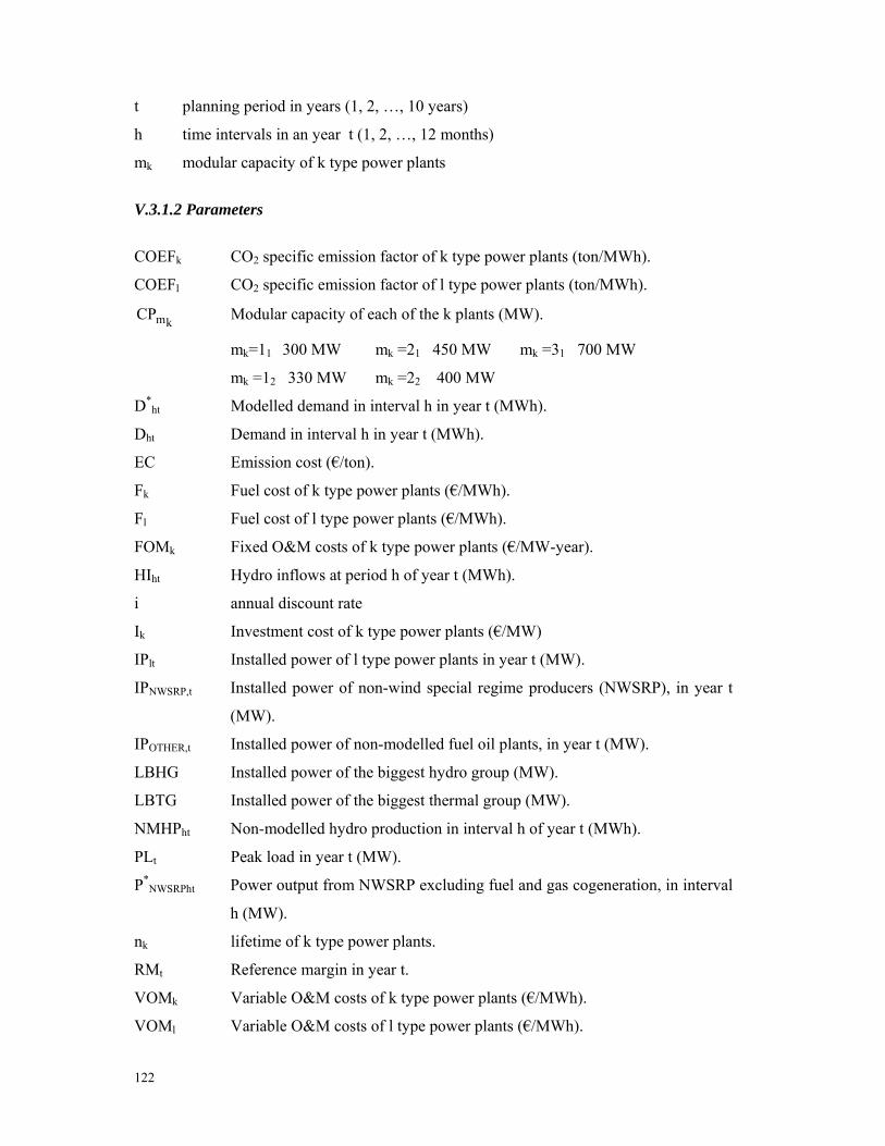
122

t planning period in years (1, 2, …, 10 years)

h time intervals in an year t (1, 2, …, 12 months)

mk modular capacity of k type power plants

V.3.1.2 Parameters

COEFk CO2 specific emission factor of k type power plants (ton/MWh).

COEFl CO2 specific emission factor of l type power plants (ton/MWh).

kmCP Modular capacity of each of the k plants (MW).

mk=11 300 MW mk =21 450 MW mk =31 700 MW

mk =12 330 MW mk =22 400 MW

D*ht Modelled demand in interval h in year t (MWh).

Dht Demand in interval h in year t (MWh).

EC Emission cost (€/ton).

Fk Fuel cost of k type power plants (€/MWh).

Fl Fuel cost of l type power plants (€/MWh).

FOMk Fixed O&M costs of k type power plants (€/MW-year).

HIht Hydro inflows at period h of year t (MWh).

i annual discount rate

Ik Investment cost of k type power plants (€/MW)

IPlt Installed power of l type power plants in year t (MW).

IPNWSRP,t Installed power of non-wind special regime producers (NWSRP), in year t

(MW).

IPOTHER,t Installed power of non-modelled fuel oil plants, in year t (MW).

LBHG Installed power of the biggest hydro group (MW).

LBTG Installed power of the biggest thermal group (MW).

NMHPht Non-modelled hydro production in interval h of year t (MWh).

PLt Peak load in year t (MW).

P*NWSRPht Power output from NWSRP excluding fuel and gas cogeneration, in interval

h (MW).

nk lifetime of k type power plants.

RMt Reference margin in year t.

VOMk Variable O&M costs of k type power plants (€/MWh).

VOMl Variable O&M costs of l type power plants (€/MWh).

123

ϕkh Availability factor of k type power plants, in interval h.

ϕlh Availability factor of l type power plants, in interval h.

∆h Length of the interval h (number of days in a month×24 h).

χW Non usable wind capacity (%).

χH Non usable large hydro capacity under a dry regime (%).

χNWSRP Non usable NWSRP capacity (%).

V.3.1.3 Decision variables

The decision variables are the numerical quantities for which values are to be chosen in the

optimisation problem (Coello et al., 2002).

tkmθ Total number of mk modules of candidate power plants in year t (integer

variable).

IP k=3a,t Total installed power of the candidate onshore wind power plants in year t

(MW).

IP k=3b,t Total installed power of the candidate offshore wind power plants in year t

(MW).

Pkht Power output from plant type k in interval h of year t (MW).

Plht Power output from plant type l in interval h of year t (MW).

The variables obtained directly from the decision variables are:

Rht Reserve of the storage hydro power plants at the end of interval h of year t,

computed from the Pl=7,h,t (MWh).

IPkt Total installed power of the k type power plants in year t, computed from

tkmθ (MW).

V.3.1.4 Objective functions

The objectives represent the criteria used to evaluate the quality of a certain solution. The

objective functions describe mathematically the relationship between the decision

variables. In the proposed Electricity Planning Model (EPM), the two objective functions

124

are measured in different units and the aim is to find the optimum between economic and

environmental aspects.

C Total present value of cost (€).

CO Total CO2 emissions (ton).

V.3.2 Cost objective function

The cost objective function consists of the total present value of cost (C), which includes:

The fixed cost (FC), corresponding to the present worth of the investment cost (Ik)

and fixed operation and maintenance costs (FOMk) of the candidate plants.

The variable cost (VC), corresponding to the present worth of the variable O&M,

fuel and emission costs of the existing, future and candidate plants,

C = FC + VC (€) (5.1)

The cost values of the plants may be found in Tables 5.2 and 5.4; the analysed year is

divided in H intervals of duration, each one characterized by the demand power.

The capital investment cost is obtained for all the candidate power plants as a sum of the

annuities over the planning period. The calculations are based on the uniform distribution

of the investment cost during the plant lifetime and assume that this cost is incurred in the

first year of the plant operation. The decommissioning cost was set equal to the final

salvage value of the installations resulting in a null value.

The formula for the annualised cost (AC) of the present value of the investment cost (Ik)

over the period of plant lifetime (nk) at a given discount rate (i) is given by:

1i)(1i)i(1IACkn

kn

k−+

+= (5.2)

The total FOMk costs are also obtained for all the candidate power plants as a sum of the

annual values over the planning period. As both the investment and FOMk costs are set as a

125

function of the total installed power of each plant type, the cost values must be multiplied

by the total installed power of each power plant in each year.

For the existing power plants, the model assumes that the fixed O&M costs will always be

incurred regardless of the power plant being or not used in the entire planning period.

Although the plant may not be required to operate during the planning period it is assumed

that these plants will still be available as reserve. As such the fixed O&M costs for the

existing power plants are not included in the optimisation process.

The fixed cost may be described then as:

( )∑∑⎪⎭

⎪⎬⎫

⎪⎩

⎪⎨⎧

+×⎥⎦

⎤⎢⎣

⎡+

−++

= −

t k

tktkn

n

k i1 IPFOM1i)(1

i)i(1IFCk

k

(€) (5.3)

Due to the short planning period considered (10 years) no construction times were taken

into consideration. Also, there are no restrictions on the number of available groups in the

market to supply in each year. In the future, if forecasts for the electricity system for a

longer period become available, it will be possible to change the present models

introducing these new data and additional constraints that will take into consideration the

plant construction time and the availability limitations of the market.

The total variable costs are obtained as the sum of the variable costs of each power plant

(candidate and existing) during the planning period. The variable costs depend on the

amount of electricity produced. As so, these specific cost values must be multiplied by the

electricity produced by each power plant in each month. This production is obtained by the

multiplication of the power output (Pkht and Plht, measured in MW) by the length of the

interval measured in hours (∆h=number of days in month h × 24h). The variable cost

includes the variable O&M costs, the fuel consumption (coal, natural gas and fuel oil) and

the economic value of the CO2 emissions. This last element is based on the specific

emission factor56 of each technology (COEFk or COEFl) and on the market value of the

CO2 allowances (EC), obtained from information drawn from the websites of the organized

markets (EEX, EXAA and NordPool).

56 Specific CO2 emission factor is the amount of CO2 released per unit of electricity produced (ton /MWh)

126

( ) ( )[ ]( ) ( )[ ]∑∑∑

∑∑∑−

−

+××××+++

+××××++=

t h l

thlhtlll

t h k

thkhtkkk

i1 ∆PCOEFECFVOM

i1∆PCOEFECFVOMVC (€) (5.4)

Combining equations 5.1, 5.3 and 5.4 the total cost function may be described as follows:

( )

( ) ( )[ ]( ) ( )[ ]∑∑∑

∑∑∑

∑∑

×+×××+++

×+×××+++

⎭⎬⎫

⎩⎨⎧

+×⎥⎦

⎤⎢⎣

⎡+

−++

=

−

−

−

t h lh

tlhtlll

t h kh

tkhtkkk

t k

tktknk

nk

k

∆i1PCOEFECFVOM

∆i1PCOEFECFVOM

i1 IPFOM1i)(1

i)i(1IC

(€) (5.5)

The total cost value depends on the specific costs previously defined for each technology

but also on the interest rate set by the decision maker. This function assumes constant

prices, no increase rate of the O&M and no increase rate of fuel costs during the planning

period. The final value obtained from equation 5.5, corresponds to the present worth of the

expected costs for the next 10 years.

Costs for grid extensions are not accounted for in these cost calculations. The question of

the grid costs is particularly important for the Portuguese electricity system, due to the

prevalence of wind resources in inland hills with underdeveloped grid structures. However,

as the model makes no assumptions on the location of candidate plants and due to the lack

of information concerning grid extension costs, this cost element was not included in the

analysis.

V.3.3 Emissions objective function

For the emissions objective function, CO2 values are used as a rough proxy of the pollutant

emissions. Directive 2001/80/EC focus already on the limitations of emissions of SO2,

particulate and NOx from large combustion power plants, which is leading to the adoption

of measures for their reduction (both Sines and Pego coal power plants have already

presented proposals for desulphurisation projects). It seemed more relevant for the moment

to focus on the CO2 values due to the existence of clear objectives for Portugal, set by the

Kyoto protocol. This protocol recognises CO2 as the most important greenhouse gas

(GHG). It should be however highlighted that future developments of the model may

127

accommodate other pollutant emissions as additional objectives.

For the computation of the total CO2 emissions, a specific emission factor for each

technology was assumed for the existing and candidate power plants (COEFk or COEFl).

The total emissions are obtained as the sum of the emissions of each power plant during

the planning period. These emissions are a linear function of the electricity produced by

each power plant in each month.

( )[ ] ( )[ ]∑∑∑∑∑∑ ××+××=t h l

hlhtlt h k

hkhtk ∆PCOEF ∆PCOEFCO (ton) (5.6)

The first term of equation 5.6 represents the sum of the monthly emissions, released by the

candidate power plants during the planning period. The second term accounts for the sum

of the monthly emissions, released by the existing and commited power plants during the

planning period. The final value obtained from this equation, corresponds to total CO2

emissions expected to be released during the next 10 years.

V.3.4 Constraints

The constraints of the problem describe mathematically the restrictions imposed by the

particular legal characteristics of the system, by the expected demand and load, by the

technical characteristics of the power plants involved and by the security of supply

assurance. These restrictions must be satisfied in order to accept the solution or solutions

found as feasible. The EPM model includes inequality and equality constraints. The

constraints described in the next sections define then the feasible region of the problem.

V.3.4.1 Demand constraints

In each interval of the planning period, the electricity production must be larger than or

equal to the demand. The number of these constraints is 120. The excess of production, if

existing, may be used for exportations or for electricity storage using reversible hydro

schemes for example. The value of this excess production is assumed to be zero.

th,h

ht*

llht

kkht

∆DPP ∀≥+∑∑ (MW) (5.7)

128

The left side of the equation represents the total power output from all the existing and

candidate power plants in a given month (h) of a given year (t) of the planning period. The

right side of the equation represents the total modelled power demanded for the same

interval. This modelled power demanded is obtained by the division of the electricity

demand in that given interval (D*, measured in MWh), by the length of the interval

(measured in hours). The monthly D* values may be found in Annex 4.

V.3.4.2 Power capacity constraints

In each interval of the planning period, the production of each power plant may not exceed

its production capacity multiplied by its availability factor. The number of these constraints

is 720.

th, 3b, and 3akktkhkht IPP ≠∀≤ ϕ (MW) (5.8)

th, 7, and 9lltlhlht IPP ≠∀×≤ ϕ (MW) (5.9)

For k=3a and 3b and l=9 (wind power) see equations 5.15-5.17. For l=7 (hydro power) see

equations 5.20-5.24.

The left term of equations 5.8 and 5.9 represent the power output of a candidate or existing

power plant (k or l) in a given month (h) of a given year (t) of the planning period. The

right side of the equation represents the available power for that power plant in that

particular interval, depending on the installed power and on the availability factor (ϕkh and

ϕlh) of the generating unit.

The availability factor is computed as the ratio between the average available power in

each month and the installed power for each generating unit. For the thermal power plants

it was assumed that ϕ would be kept constant during the entire year and would be

independent from the number of installed plants in the system. It was assumed an

availability factor of 95% for each thermal power plant type, based on past records (EDP,

2004b). The wind and hydro power constraints will be treated independently, as described

in Sections 3.4.5 and 3.4.7.

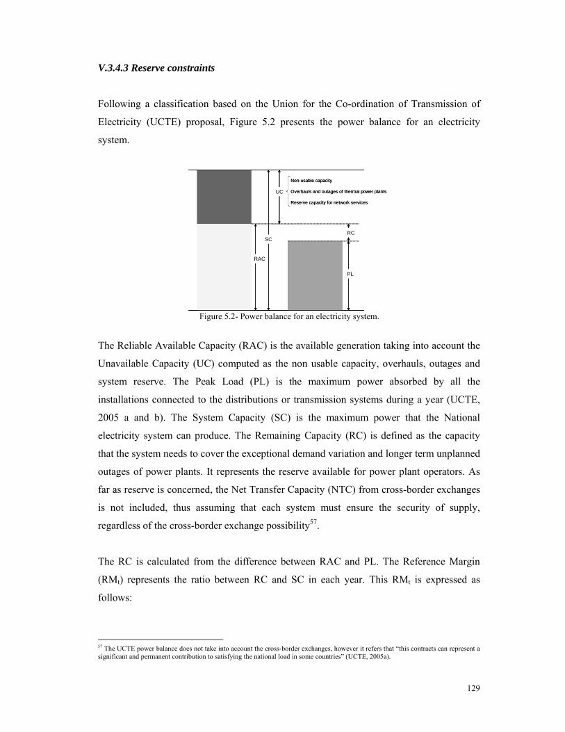
129

V.3.4.3 Reserve constraints

Following a classification based on the Union for the Co-ordination of Transmission of

Electricity (UCTE) proposal, Figure 5.2 presents the power balance for an electricity

system.

SC

RAC

RC

PL

UC

Non-usable capacity

Overhauls and outages of thermal power plants

Reserve capacity for network services

SC

RAC

RC

PL

UC

Non-usable capacity

Overhauls and outages of thermal power plants

Reserve capacity for network services

Figure 5.2- Power balance for an electricity system.

The Reliable Available Capacity (RAC) is the available generation taking into account the

Unavailable Capacity (UC) computed as the non usable capacity, overhauls, outages and

system reserve. The Peak Load (PL) is the maximum power absorbed by all the

installations connected to the distributions or transmission systems during a year (UCTE,

2005 a and b). The System Capacity (SC) is the maximum power that the National

electricity system can produce. The Remaining Capacity (RC) is defined as the capacity

that the system needs to cover the exceptional demand variation and longer term unplanned

outages of power plants. It represents the reserve available for power plant operators. As

far as reserve is concerned, the Net Transfer Capacity (NTC) from cross-border exchanges

is not included, thus assuming that each system must ensure the security of supply,

regardless of the cross-border exchange possibility57.

The RC is calculated from the difference between RAC and PL. The Reference Margin

(RMt) represents the ratio between RC and SC in each year. This RMt is expressed as

follows:

57 The UCTE power balance does not take into account the cross-border exchanges, however it refers that “this contracts can represent a significant and permanent contribution to satisfying the national load in some countries” (UCTE, 2005a).

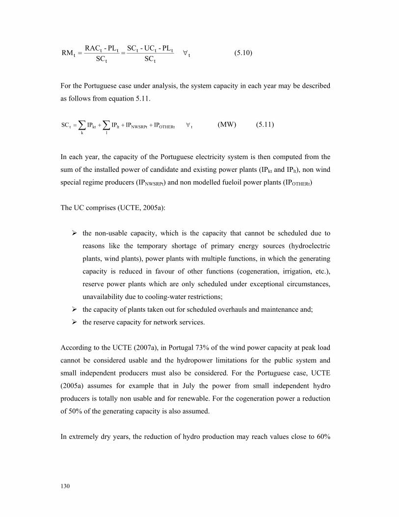
130

SC

PL-UC-SC SC

PL-RACRM tt

ttt

t

ttt ∀== (5.10)

For the Portuguese case under analysis, the system capacity in each year may be described

as follows from equation 5.11.

IPIPIP IPSC tOTHERtNWSRPtl

ltk

ktt ∀+++= ∑∑ (MW) (5.11)

In each year, the capacity of the Portuguese electricity system is then computed from the

sum of the installed power of candidate and existing power plants (IPkt and IPlt), non wind

special regime producers (IPNWSRPt) and non modelled fueloil power plants (IPOTHERt)

The UC comprises (UCTE, 2005a):

the non-usable capacity, which is the capacity that cannot be scheduled due to

reasons like the temporary shortage of primary energy sources (hydroelectric

plants, wind plants), power plants with multiple functions, in which the generating

capacity is reduced in favour of other functions (cogeneration, irrigation, etc.),

reserve power plants which are only scheduled under exceptional circumstances,

unavailability due to cooling-water restrictions;

the capacity of plants taken out for scheduled overhauls and maintenance and;

the reserve capacity for network services.

According to the UCTE (2007a), in Portugal 73% of the wind power capacity at peak load

cannot be considered usable and the hydropower limitations for the public system and

small independent producers must also be considered. For the Portuguese case, UCTE

(2005a) assumes for example that in July the power from small independent hydro

producers is totally non usable and for renewable. For the cogeneration power a reduction

of 50% of the generating capacity is also assumed.

In extremely dry years, the reduction of hydro production may reach values close to 60%

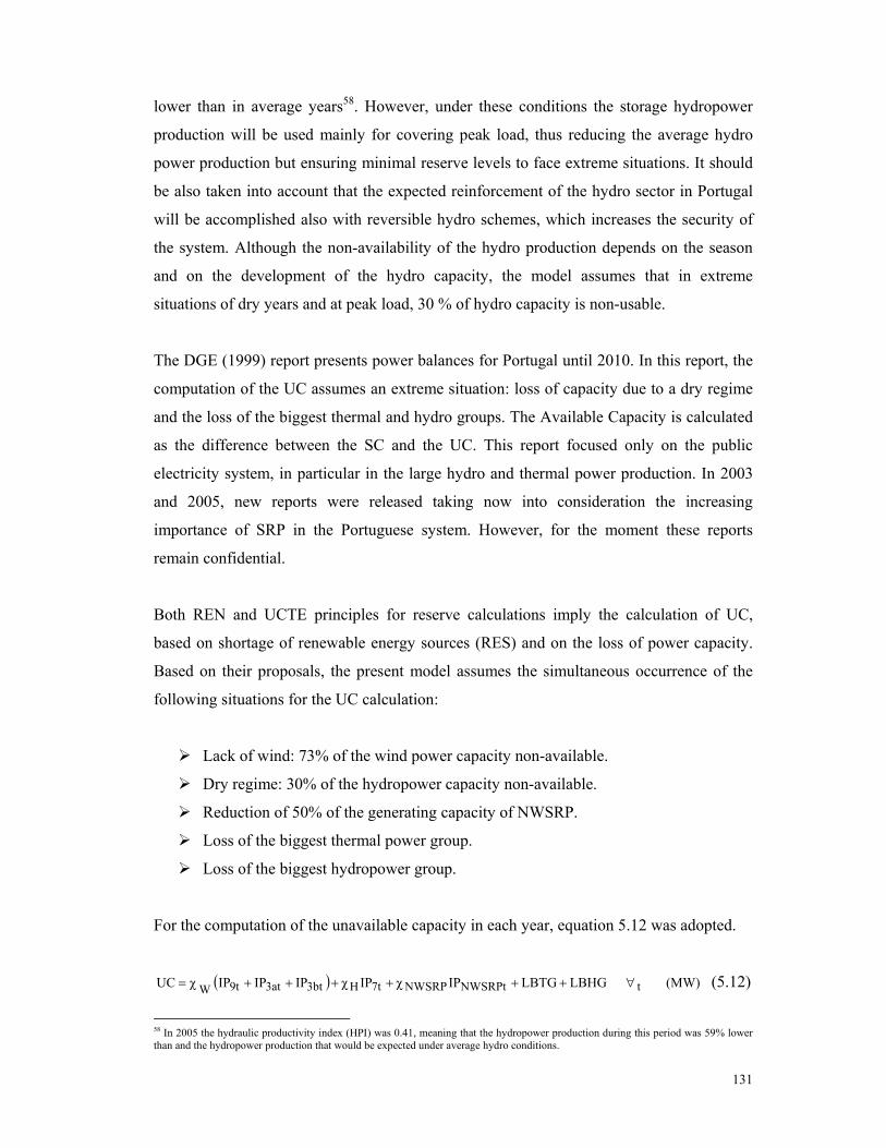
131

lower than in average years58. However, under these conditions the storage hydropower

production will be used mainly for covering peak load, thus reducing the average hydro

power production but ensuring minimal reserve levels to face extreme situations. It should

be also taken into account that the expected reinforcement of the hydro sector in Portugal

will be accomplished also with reversible hydro schemes, which increases the security of

the system. Although the non-availability of the hydro production depends on the season

and on the development of the hydro capacity, the model assumes that in extreme

situations of dry years and at peak load, 30 % of hydro capacity is non-usable.

The DGE (1999) report presents power balances for Portugal until 2010. In this report, the

computation of the UC assumes an extreme situation: loss of capacity due to a dry regime

and the loss of the biggest thermal and hydro groups. The Available Capacity is calculated

as the difference between the SC and the UC. This report focused only on the public

electricity system, in particular in the large hydro and thermal power production. In 2003

and 2005, new reports were released taking now into consideration the increasing

importance of SRP in the Portuguese system. However, for the moment these reports

remain confidential.

Both REN and UCTE principles for reserve calculations imply the calculation of UC,

based on shortage of renewable energy sources (RES) and on the loss of power capacity.

Based on their proposals, the present model assumes the simultaneous occurrence of the

following situations for the UC calculation:

Lack of wind: 73% of the wind power capacity non-available.

Dry regime: 30% of the hydropower capacity non-available.

Reduction of 50% of the generating capacity of NWSRP.

Loss of the biggest thermal power group.

Loss of the biggest hydropower group.

For the computation of the unavailable capacity in each year, equation 5.12 was adopted.

( ) (MW) LBHG LBTGIPχIPχIPIPIPχUC tNWSRPtNWSRP7tH3bt3at9tW ∀++++++= (5.12)

58 In 2005 the hydraulic productivity index (HPI) was 0.41, meaning that the hydropower production during this period was 59% lower than and the hydropower production that would be expected under average hydro conditions.

132

The right side of the equation represents the sum of:

the reduction of wind power due the lack of wind (χW)

the reduction of hydro power due to a dry regime (χH),

the loss of part of the NWSRP power (χNWSRP) and,

the loss of the biggest thermal and hydro power groups . (LBTG and LBHG)

The system must also have a level of operational reserve power for unexpected variations

in supply or demand, typically in a time range of less than one hour. For the identification

of the proper means for energy production the time necessary for the mobilisation of the

reserve power and the load variation gradients must be considered (Esteves, et al., 2003).

REN studies (Esteves et al., 2003) indicate that, if the installed wind power in Portugal

reaches 4150 MW, wind power variations in a time range of one hour can be above 1100

MW. REN recommends the use of hydro pumping schemes to ensure the rapid

mobilization of the operational power reserve, allowing also for hydro pumping in periods

of higher source affluence and simultaneously contributing to the accomplishment of the

renewable objectives. Additionally, the last REN investment plan (REN, 2005) already

forecasts the installation of three single cycle gas turbine groups to work as peak units.

Figure 5.3 shows the Portuguese power balance in 2016, according to REN (2005)

projections.

SC = 22.8 GW

RAC15.2 GW

RC = 1.2 GW

PL = 14 GW

UC

Non-usable capacity: 6.8 GW

Loss of the biggest thermal group: 450 MW

Loss of the biggest hydro group: 315 MW

SC = 22.8 GW

RAC15.2 GW

RC = 1.2 GW

PL = 14 GW

UC

Non-usable capacity: 6.8 GW

Loss of the biggest thermal group: 450 MW

Loss of the biggest hydro group: 315 MW

Figure 5.3- Expected power balance for the Portuguese electricity system in 2016. Source: Own elaboration of REN (2005) data. Combining Figure 5.3 information with equation 5.10 the value of the RM for the REN

133

(2005) scenario in 2016 (reference scenario) may be computed:

0.05 22.8

14-15.2RM t == for t=2016, under REN scenario

For the model formulation, it will be assumed that in each year the value of the RM must

be at least equal to the value obtained under the reference scenario. Combining equations

5.10, 5.11 and 5.12 the expression for the reserve constraint may be obtained:

( )[ ]

IPIPIP IP

PL -LBHGLBTGIPχIPχIPIPIPχIPIPIPIP05.0 t

OTHERtNWSRPtl

lk

kt

ltNWSRPtNWSRP7tHt3b,t3a,9tOTHERtNWSRPtlt

kkt W

∀+++

++++++−+++≤

∑∑∑∑

(5.13)

The number of these constraints in the model is equal to 10. As mentioned, the minimum

value of RMt is parameter of the model, set according to the reference scenario obtained

from REN (2005) forecasts for 2016.

V.3.4.4 Renewable constraints

Directive 2001/77/EC states that after 2010, 39% of the Portuguese electricity consumption

must come from RES. Given the large share of hydroelectricity production in Portugal, the

rainfall is the climate factor with the strongest impact on electricity production from RES.

Using an approach followed in the Portuguese reports in the frame of this Directive, hydro

production will be corrected by the hydraulic productivity index (HPI) (equal to 1.22) of

the base year of the Directive (1997). The Renewable constraint is expressed as follows:

( )[ ](5.14) 0.39

D

NMHP 22.1 ∆PP 22.1 PPP

3t

hht

hhth

*NWSRPht7ht9htht3b,ht3a,

≥∀≥+×++++

∑∑

HPI1997

( )[ ](5.14) 0.39

D

NMHP 22.1 ∆PP 22.1 PPP

3t

hht

hhth

*NWSRPht7ht9htht3b,ht3a,

≥∀≥+×++++

∑∑

HPI1997

The numerator of equation 5.14 represents the total production from RES in a given year t,

134

including:

electricity production from candidate wind power plants (obtained from P3a,ht,

P3b,ht) and electricity production from existing wind power plants (P9ht),

modelled electricity production from hydro storage power plants (obtained from

P7) and non modelled electricity production from hydro power plants (NMHP) and,

electricity production from NWSRP excluding fuel and gas cogeneration

(obtained from P*NWSRP and presented in Annex 5).

The denominator of the equation represents the total electricity demand in the same given

year (t). This ratio must be at least equal to 39% for every year after 2010, which is the

same as saying for t≥3. The number of these constraints is equal to 8.

This renewable constraint sets the minimum share of the electricity produced from RES

equal to 39%. This limit represents a parameter of the model that may change due to legal,

political or technical reasons in the next years. For example, as mentioned before the

European Commission (Commission of the European Communities, 2007) proposed

already new targets to increase the level of renewable energy in the EU’s overall mix to

20% in 2020, which will require the drawing of new objectives for each Member State’s

electricity sector.

V.3.4.5 Wind constraints

According to the present regulations of the Portuguese electricity sector, renewable energy

production has priority dispatch and the electricity produced from RES is always accepted

to the grid. The mathematical formulation of this legal protection to wind power is

presented by equality constraints described by equations 5.15- 5.17:

h t,t3a,h3a,ht3a, IPP ∀×= ϕ (MW) (5.15)

h t,t3b,h3b,ht3b, IPP ∀×= ϕ (MW) (5.16)

IPP h t,9t9h9ht ∀×= ϕ (MW) (5.17)

135

The wind power output in each interval (h) of each year (t) is set equal to the available

capacity. This available capacity depends on the installed wind power (IP3a,t, IP3b,t and IP9t)

in each year and on the availability factor of wind in each month (ϕ3a, ϕ3b and ϕ9). These

monthly values reflect the wind seasonality and were computed as the average of the

values recorded during the last six years (2001-2006)59. Due to the inexistence of

information in regard to the availability factor of offshore and future onshore wind power

plants, ϕ3a and ϕ3b were set equal to ϕ9 in the model. Annex 3 presents these values. The

number of these equality constraints is equal to 360.

V.3.4.6 Plant capacity constraints

For the thermal power plants, a limited set of modular capacities in the market were

assumed. Thereby, for each year the total installed power of the candidate PCSC and

CCGT plants must be equal to an integer value multiplied by the available modular

capacities of the candidate plants. The number of these constraints is equal to 20.

3b and 3ak t,m

mtmkt CPθIPk

kk ≠∀×= ∑ (MW) (5.18)

The capacities for each technology were previously defined and included as parameters in

the model ( kmCP , in MW). tkmθ , is a variable describing the number of units with

capacity equal to kmCP installed between the beginning of the planning period and year t.

No impositions were made in regard to the number of modules available in the market in

each year.

As IPkt represents the total installed power of k type power plants available in the system in

year t, a new constraint must be added to the system ensuring that the value of IPkt is

increasing during the planning period.

3b and 3ak 2,t1-ktkt IPIP ≠≥∀≥ (5.19)

The number of these constraints is equal to 18.

59 Values computed from information drawn from REN website (www.ren.pt).

136

V.3.4.7 Hydro constraints

The hydro constraints are based on the initial reserves on the hydro storage hydro plants

and the expected inflows. The hydro storage reserve at the end of a given month (Rht,

measured in MWh) must be equal to the reserve at the beginning of the month (Rh1,t) plus

the hydro inflows to the plant in that given month (HIht,measured in MWh), subtracted by

the plant production in that period (computed by the power output P7h,t and by the number

of hours in the month ∆h). The mathematical formulation of the constraint involves two

different equations: one for January, depending on the reserve values of December of the

previous year (equation 5.20) and another one for the other eleven months, depending on

the reserve values of the previous month in the same year (equation 5.21).

1h t,1ht1,h7,t1,h1-t12,ht1,h ∆PHIRR ====== ∀×−+= (MWh) (5.20)

1h t,hht7,htt1,-hht ∆PHIRR ≠∀×−+= (MWh) (5.21)

The initial reserve is assumed to be equal to the value in the beginning of 2006. The

monthly inflows were computed based on the average values between 2001 and 2006 and

on the expected increase of the installed capacity of the hydro power sector60. These

monthly inflows may be found in Annex 6. It was also assumed that the final value of the

reserve (December 2017) should be equal to the initial one. These initial value was set as a

parameter in the model.

reserve InitialR12,10 = (MWh) (5.22)

The number of these constraints is equal to 120. A minimum and maximum reserve levels

were also assumed, avoiding the model to unrealistically accommodate water or to

completely deplete all the water reserves. For this two additional constraints were included

for each month of each year:

60 Values computed from information drawn from REN website (www.ren.pt). It should be highlighted that most of the 2001-2006 years present HPI below the average and are strongly influenced by an extremely wet year (2005), which may lead to some underestimation of the expected hydroelectricity production.

137

h t,ht 1200000R ∀≥ (MWh) (5.23)

h t,ht 0000003R ∀≤ (MWh) (5.24)

This value was estimated from the minimum levels presented in 2005 and from the

maximum levels computed from REN monthly statistics information61.

V.3.4.8 Natural gas constraint

The operating characteristics of the Portuguese electricity system described in Section II.4

of this thesis, indicate that coal power plants output should be relatively stable and CCGT

although being mainly operated as baseload units are able to provide a little more

flexibility to the system. It seems then unrealistic to think that during a month the power

production could come only from coal power plants, SRP and hydro power plants as this

would necessarily imply significant variations on coal power output and/or a very

favourable hydro regime.

Ideally the model should include a constraint ensuring a minimum operating regime for

each coal power plant. However, the present model does not deal with individual power

plants and data are aggregated in monthly values, which create difficulties on the definition

of operating constraints. To tackle this problem and with the aim of preventing unrealistic

solutions, a proxy constraint was used ensuring that at least a minimal amount of electricity

would come from CCGT operation every month. During 2006, the electricity production

from CCGT reached the minimum level in November equivalent to an average power

output of 310 MW62. It was then decided to set the minimal electricity production from

CCGT equal to the average power output of that month:

th,ht5,ht2, 310 PP ∀≥+ (MW) (5.25)

61 Source: www.ren.pt 62 Source: Monthly information drawn from REN site.

138

V.3.4.9 Bound constraints

All the production values must be positive, tmkθ is also a positive and integer variable.

riableInteger va 0θ

0P

0P

tm

th,l,k,khl

kht

k≥

∀≥

≥

(5.26)

The total installed wind power should not overcome the assumed wind potential, based on

the environmental and economic viability of these power plants. Esteves et al.’s (2003)

study indicates an onshore wind potential of about 7700 MW, assuming more than 2500

full load hours. In 1993, Van Wijk and Coelingh (EWEA, 2005b) assessed the technical

onshore wind resource for OECD countries and indicated the value of 15 TWh/year for

Portugal. Assuming 2500 full load hours availability, this value corresponds to about 6000

MW of installed capacity. However, due to the development of the wind technology this

value may now be too conservative.

For this study an onshore wind potential for Portugal of about 8000 MW was assumed.

Taking into account that by the end of 2006 about 1500 MW were already installed, the

limit to the total installed power for onshore wind power plans (IP3a,t) was set equal to

6500 MW.

To the authors knowledge there are not many studies focusing on offshore wind potential

in Portugal. The Commission funded CA-OWEE project (Concerted action on offshore

wind energy in Europe) (EWEA, 2005b) estimates 2-3 TWh/year as the offshore wind

potential for Portugal. Assuming 2500 full load hours, this value corresponds to installed

wind power of 800 to 1200 MW. Estanqueiro (2006) indicated that the offshore potential

should be higher than 1000 MW in Portugal. For the present study a conservative estimate

of 1000 MW was assumed as the offshore wind potential in Portugal. Accordingly the total

installed power for offshore wind power plans (IP3bt) must not be greater than 1000 MW.

139

1000IP0

6500IP0

3bt

t

3at

≤≤∀

≤≤ (MW) (5.27)

V.3.5 Final considerations

Figure 5.4 shows the flow diagram for the EPM, including the input information, output

results and the optimisation problem.

Average SFC1

Average COEF2

Coal

Fueloil

SCGT

CCGT

1 Specific fuel consumption2 CO2 emission factor

Cost

CO2

Objectives

Demand

Legal

System

Constraints

Electricity production plan

CO2 production

Cost

Capacity expansion plan

Results

Plant

Load

Data

GAMS code

Cost

CO2

Objectives

Demand

Legal

System

Constraints


CO2 production

Cost


Results

Plant

Load

Data

GAMS code

Average SFC1

Average COEF2

Coal

Fueloil

SCGT

CCGT


Cost

CO2

Objectives

Demand

Legal

System

Constraints


CO2 production

Cost


Results

Plant

Load

Data

GAMS code

Cost

CO2

Objectives

Demand

Legal

System

Constraints


CO2 production

Cost


Results

Plant

Load

Data

GAMS code

Figure 5.4- Electricity planning model.

The input information for the problem includes the mathematical formulation of the

objectives and constraints. These constraints may be classified as:

Demand, ensuring that the demand for electricity is always met over the planning

horizon.

Legal, representing the legal and political impositions to the system (renewable and

wind constraints).

System, which take into account the technical characteristics of the system and of

the power plants (capacity, reserve, hydro and natural gas).

The input data describes the technical and economic characteristics of the existing and

candidate power plants and the expected load (demand) pattern. This linear model assumes

140

average specific fuel consumption63 and CO2 emission factors for each type of thermal

power plant. Annexes 1 to 6 present the data used in the model, including installed power

of the existing power plants, average and peak load, NWSRP, average hydro inflows and

the computation of the estimated modelled demand. The proposed model includes the

following data modules:

Information on all the generating units in the system at the start of the study and a

list of retirements and fixed additions to the system.

Information on the various generating units to be considered as candidates for

expanding the generating system.

Information on demand, peak load for the planning period and the previously

committed production (non-modelled).

The model does not deal with individual power plants but with technologies. Average

values for the efficiency, CO2 emission factors and specific fuel consumption are

considered for each technology based on the average operating conditions occurred in

previous years (for existing power plants) and on the expected performance of future

power plants. It should be also underlined that the model does not foresee compensation

payments for plants that although not producing or producing very little during the

planning period would still be available as reserve. The model assumes that the fixed

O&M will always be incurred even for these non-operational power plants.

The proposed EPM was written in a GAMS (General Algebraic Modelling System) code

compiling all the data and calling an optimising solver according to the model

characteristics. Table 5.5 summarises other general assumptions considered under the base

scenario of the EPM.

The problem resulted in a multivariable constrained mixed integer linear programming

(MILP) model that involves several variables both continuous and integer and is linear in

the objective functions and the constraints.

63 Specific fuel consumption is the amount of fuel consumed per unit of electricity produced (m3N/MWh for CCGT and ton/MWh for coal and fueloil).

141

Table 5.5- General assumptions of the EPM Planning period 2008-2017 Costs expressed in € of 2005 base year Portuguese GDP deflator. Source: Eurostat. Real discount rate 5%.*

CO2 emission costs 22 €/ton* Average value at the beginning of 2006. Source: EEX, EXAA and NordPool.

Coal cost 56.7 €/ton* Source: EDP (2006b)Natural gas cost 241 €/103m3N* Source: EDP (2006b) Fueloil cost 202.6 €/ton Demand sub-periods Monthly Reference Margin 5% REN scenarios for 2016 (see Section V.3.4.3) Initial reserve 1437 GWh Source: REN site (January 2006) * Changes considered under sensitivity analysis.

V.4 The optimisation process

Problems in engineering, economics, physics and social sciences often involve several

objectives. If these objectives are opposing, it is necessary to find the best possible solution

that satisfies the opposing objectives subject to certain restrictions. A multiobjective

optimisation problem may have a possible uncountable set of solutions, which when

evaluated produce vectors whose components represent trade-offs in objective space. The

aim of this kind of problems is to find good compromise solutions. The set of variables that

produces the optimal outcome is designated as the optimal set and is referred to as the

Pareto optimal.

The Pareto optimal of a problem may be defined as (Coello et al., 2002):

“(..) *xr is a Pareto optimal if there exists no feasible vector xr which would decrease some

criterion without causing a simultaneous increase in at least some other criterion (..)”

The region of points formed by the Pareto optimal solutions is called the Pareto front. The

decision maker’s task in a multiobjective problem is to select compromise solutions drawn

from the Pareto front. This selection depends on the acceptable objective performances,

according to the decision maker’s point of view. Figure 5.5 represents the Pareto front for

an example of a problem with two objectives (f1 and f2).

142

Pareto front

Feasible region

f2

f1

Pareto front

Feasible region

f2

f1 Figure 5.5- Pareto front for a problem with two objective functions.

The objective of the research is now to find the Pareto front for the bi-objective EPM.

Optimisation manuals like Coello et al. (2002) or Collette and Siarry (2003), present a

description of the available multiobjective optimisation techniques currently in use. For

this particular model, the ε constraint method or trade-off method will be used. This

method consists in the minimisation of one objective at a time, considering the other as

constraints bounded by allowable levels (ε).The Pareto front can be found by varying these

levels.

Following Coello et al.’s (2002) notation, for a problem with a vector xr of n decision

variables and a vector ( )xf rr of k objective functions:

⎥⎥⎥⎥

⎦

⎤

⎢⎢⎢⎢

⎣

⎡

=

nx

xx

x..

2

1

r and ( )

( )( )

( )⎥⎥⎥⎥

⎦

⎤

⎢⎢⎢⎢

⎣

⎡

=

xf

xfxf

xf

kr

r

r

rr

..2

1

the trade off method may be represented as:

( )xfrrr

min

subject to:

( ) r lkxf ll ≠=≤ and 1,2,...,lfor εrr

This method was chosen for three main reasons:

the problem involves only two objectives, generating a limited set of combinations

143

that will result in a set of solutions that can reasonably describe the Pareto front.

The method is especially suited for this particular case because the allowable levels

for CO2 may be drawn directly from the Kyoto objectives for Portugal.

no particular assumption has to be made on the cost objective, since the Pareto

front will derive from the minimisation of the cost objective and varying the CO2

allowable levels.

With this approach the multiobjective model will be treated as a constrained single

objective problem. The cost function will be the primary objective and the CO2 function

will be treated as a constraint. Varying the CO2 allowable levels will make possible

obtaining a set of solutions representing trade-offs between cost and environment.

A preliminary analysis was performed to identify the proper boundaries for the minimum

allowable levels which also allowed the analysis of the degree of conflict of the two

objectives. For this, independent single-objective optimisations were carried out for each

objective function.

To solve the EPM, the model was described in a GAMS code. This language is specially

suited to solve large linear, nonlinear and mixed integer optimisation problems. It makes

possible to call for different solvers according to the specific characteristics of the problem.

A more detailed description of this programming language and some examples of GAMS

models may be found in the web page (www.gams.com) and in the users’ guides Rosenthal

(2006) and McCarl (2006).

For this particular model the Branch and Bound (BB) algorithm was used. This is one of

the most common approaches to solve mixed integer linear and non linear problems

(Winston, 1994 and Murray and Shanbhag, 2007) and it is also recommended by GAMS

solvers to solve large problems. The BB method uses a partitioning method for the

decision variables to divide all the feasible solutions into subsets and serially searches for

the optimum solutions for the most promising subsets. It includes a group of procedures

that attempts to perform the enumeration intelligently, so that not all combinations of

variables need to be examined.

144

The optimisation process starts with obtaining the relaxed solution of the problem. If this

solution satisfies all the integer requirements the process is finished and the solution is

returned as the optimal integer. If an integer solution is not realised, the feasible region for

the discrete variables is subdivided (branching) and bound on these discrete variables are

tightened to new integer values to cut off the current non-integer solutions.

The searching procedure is terminated by a tolerance criterion previously defined by the

user, computed in GAMS as the relative gap between the found solution and the estimated

best solution (usually obtained by the solver from the relaxed problem). For example if the

user sets this tolerance equal to 0.05, the process will stop when a solution is found within

5% of the best guess global optimum.

A detailed description of the BB method may be found in Edgar and Himmelblau (1989),

in the Baron solver manual (Sahinidis, 2000) or in Jensen and Bard (2003).

According to GAMS web information, BARON (Branch and Reduced Optimisation

Navigator) solver is suitable for searching for the global optimal of a mixed integer linear

or non linear problem. BARON is a computational system for solving optimisation

problems to global optimality. Purely continuous, purely integer, and mixed-integer

nonlinear problems can be solved with the software. It implements deterministic global

optimisation algorithms of the branch and bound enhanced type that are guaranteed to

provide global optimal, under the availability of finite lower and upper bounds on the

variables. Neumaier et al. (2005) tested several complete global optimisation solvers and

concluded that among the currently available global solvers, BARON is the fastest and

most robust64. However, Murray and Shanbhag (2007) reported some problems using this

solver due to the high computational time required. In spite of the expected long time

required to solve large problems using BARON, it was decided to use this solver at least

for this linear model.

According to the above stated, the approach to the EPM involved the following main

stages:

(1) Minimisation of the CO2 objective, using the BARON solver. 64 The study did not include integer constraints in the test set.

145

(2) Minimisation of the cost objective, using the BARON solver.

(3) Definition of the CO2 allowable levels between (1) and the CO2 value

obtained with the minimisation of the cost objective (2).

(4) Minimisation of the cost objective constrained by the CO2 allowable levels,

using BARON solver

(5) Construction of the final set of optimal solutions.

The GAMS code for the EPM solver may be found in Annex 7. V.5 Results of the EPM

Firstly, independent single-objective optimisations were carried out for both cost and CO2

objective functions, thus obtaining the extreme solutions. Each one of these solutions

corresponds to a different generating system combining different technologies and

production strategies: one for the least costly solution and another for the lower emissions

solution. The aim was to obtain the extreme solutions, described by the cost and CO2

values and the capacity expansion plans. These first results are shown in table 5.6. The

elements in the main diagonals (in grey) represent the ideal values and the other elements

indicate the corresponding value for the other objective. The results are presented both in

absolute values, corresponding to the total cost and emissions for the ten years planning

period, and unit values, corresponding to the cost and CO2 emission values per MWh

produced.

As mentioned before, for the problem optimisation we used BARON global solver and the

relative optimality tolerance (Optcr) was set equal to 0%. Table 5.6- Results of the single objective optimisation.

Absolute values Unit values Cost (M€) CO2 (Mton) Cost (€/MWh) CO2 (ton/MWh)

Optimal cost solution (S0) 16683 314.46 31.655 0.597 Optimal CO2 solution (S9) 20592 103.99 39.073 0.197

The elements in the first row indicate that the least cost solution (31.6 €/MWh)

corresponds to an average value for CO2 emissions of 0.597 ton/MWh. The elements in the

second row indicate that the least pollutant solution (0.197 ton/MWh) corresponds to an

146

average cost of about 39.1 €/MWh65. This means that the least cost solution is 19% less

expensive than the solution with lowest emissions. However, it may be observed that

corresponding emission levels are more than 3 times higher than the ones obtained with the

least CO2 solution.

The process proceeded with the bi-objective optimisation, with each of the objectives

limited by the extremes previously identified. The Pareto solutions were found from the

minimisation of the cost objective and by varying the CO2 values between the optimal CO2

solution and the value corresponding to the optimal cost solution.

As the CO2 objective is described by the total emissions expected to be released in the 10

year planning period, the equivalent constraint imposes also limits to this total value (the

Kyoto protocol establishes an average limit for the 2008-2012 period). Tightening of the

maximum allowable emission levels may be expected in the future. Instead of using

average CO2 levels for the period, if needed, the model may be easily adapted to account

for a maximum annual level.

Table 5.7 presents the results of the optimisation process. The elements in the second

column represent the absolute optimal cost solution constrained by the CO2 level indicated

in the third column. The fourth and fifth columns represent the respective unit cost and

CO2 values. The last column presents the run time for each simulation.

Table 5.7- Results of the two objective optimisation.

Cost Absolute values Unit values Run time optimisation Cost (M€) CO2 (Mton) Cost (€/MWh) CO2 (ton/MWh) (min))

S0 16683 314 31.655 0.597 159.4 S1 16905 275 32.077 0.522 39.4 S2 17075 250 32.400 0.474 18.2 S3 17259 225 32.748 0.427 115.0 S4 17531 200 33.265 0.379 114.0 S5 17837 175 33.845 0.332 177.3 S6 18254 150 34.636 0.285 25.3 S7 18814 125 35.699 0.237 6.5 S8 19414 110 36.838 0.209 14.1 S9 20592 104 39.073 0.197 0.1

All the models were formulated using GAMS and solved on a Pentium IV, 3.2 GHz

computer with 512MB memory. When setting the relatively optimally tolerance equal to

0% and depending on the runs, Baron solver took between less than a minute and close to 3 65 It should be underlined that these cost values represent average costs of the system, not comparable with marginal cost supported by the consumers and reported under daily markets.

147

hours to find the optimal solutions.

Figure 5.6 represents graphically the set of compromise solutions, corresponding to the

average cost vs. CO2 trade-off. The two extreme points of the obtained curve correspond to

the extreme solutions presented in Table 5.6.

0.0

0.1

0.2

0.3

0.4

0.5

0.6

0.7

31 32 33 34 35 36 37 38 39 40

Cost (€/MWh)

CO

2 (t/

MW

h)

Optimal cost solution

Opt

imal

CO

2 so

lutio

n

S1

S2S3

S4

S5S6

S7S8

S0

S9

Figure 5.6- Pareto curve solutions for the EPM

Table 5.8 describes the power generation expansion planning for these solutions. Table 5.9

presents the corresponding final configuration of the electricity system in 2017, described

by the total installed power for each technology and by the respective contribution for

electricity supply.

From the results it can be observed that the least cost solution points to investments mainly

in new coal power plants. New wind power appears only after 2010 due to Directive

2001/77/EC, imposing a minimum share of electricity produced from RES equal to 39% in

Portugal. According to this solution, in 2017:

The electricity supply would come mainly from new and old coal power plants.

Old and new CCGT would also be operating but representing only about 4% of the

electricity supply.

148

The remaining electricity would come from non thermal power stations namely,

wind power (about 15%), large hydro (about 14%) and NWSRP (about 11%). The

share of electricity generated by these power plants is significantly affected by

their low availability ratios. For example, the total installed wind power represents

about 23% of the total installed power but its contribution for electricity supply is

only 15%. Likewise, the large hydro power capacity represents about 24% of the

total installed power but its contribution for electricity supply is only 14%.

The electricity consumption from the renewable energy sources would represent

39% of the total electricity demand (meeting but not exceeding the renewable

Directive 2001/77/EC).

About 64% of the electricity consumption would come from imported primary

energy sources (mainly coal).

Table 5.8- Annual incremental installed power (MW) for the optimal solutions.

2008 2009 2010 2011 2012 2013 2014 2015 2016 2017 Total Coal 2250 600 700 600 300 4450

S0 Gas 330 330 Wind 1481 292 106 263 368 1666 4176 Coal 1850 750 600 700 3900

S1 Gas 330 330 Wind 10 532 992 727 963 1184 1041 826 154 28 6457 Coal 1150 300 1000 300 450 700 3900

S2 Gas 330 330 Wind 10 1531 769 685 2170 1102 190 6457 Coal 900 300 300 900 300 600 600 3900

S3 Gas 330 330 Wind 5700 775 6475 Coal 450 300 300 300 1350

S4 Gas 400 1130 660 730 2920 Wind 6500 6500 Coal

S5 Gas 990 330 1390 400 400 730 4240 Wind 6500 15 6515 Coal

S6 Gas 990 330 1390 400 400 730 4240 Wind 6500 15 6515 Coal

S7 Gas 730 660 330 330 660 660 330 660 4360 Wind 6500 6500 Coal

S8 Gas 1130 330 330 330 400 330 400 400 660 4310 Wind 6500 282 718 7500 Coal

S9 Gas 3930 330 800 400 800 800 7060 Wind 7500 7500

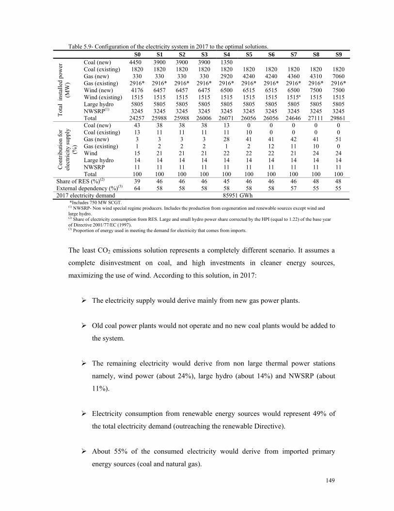
149

Table 5.9- Configuration of the electricity system in 2017 to the optimal solutions. S0 S1 S2 S3 S4 S5 S6 S7 S8 S9

Tota

l in

stal

led

pow

er

(MW

) Coal (new) 4450 3900 3900 3900 1350 Coal (existing) 1820 1820 1820 1820 1820 1820 1820 1820 1820 1820 Gas (new) 330 330 330 330 2920 4240 4240 4360 4310 7060 Gas (existing) 2916* 2916* 2916* 2916* 2916* 2916* 2916* 2916* 2916* 2916* Wind (new) 4176 6457 6457 6475 6500 6515 6515 6500 7500 7500 Wind (existing) 1515 1515 1515 1515 1515 1515 1515 1515ª 1515 1515 Large hydro 5805 5805 5805 5805 5805 5805 5805 5805 5805 5805 NWSRP(1) 3245 3245 3245 3245 3245 3245 3245 3245 3245 3245 Total 24257 25988 25988 26006 26071 26056 26056 24646 27111 29861

Con

tribu

tion

for

elec

trici

ty su

pply

(%

)

Coal (new) 43 38 38 38 13 0 0 0 0 0 Coal (existing) 13 11 11 11 11 10 0 0 0 0Gas (new) 3 3 3 3 28 41 41 42 41 51 Gas (existing) 1 2 2 2 1 2 12 11 10 0 Wind 15 21 21 21 22 22 22 21 24 24Large hydro 14 14 14 14 14 14 14 14 14 14 NWSRP 11 11 11 11 11 11 11 11 11 11 Total 100 100 100 100 100 100 100 100 100 100

Share of RES (%)(2) 39 46 46 46 45 46 46 46 48 48 External dependency (%)(3) 64 58 58 58 58 58 58 57 55 55 2017 electricity demand 85951 GWh

*Includes 750 MW SCGT. (1) NWSRP- Non wind special regime producers. Includes the production from cogeneration and renewable sources except wind and large hydro. (2) Share of electricity consumption from RES. Large and small hydro power share corrected by the HPI (equal to 1.22) of the base year of Directive 2001/77/EC (1997). (3) Proportion of energy used in meeting the demand for electricity that comes from imports.

The least CO2 emissions solution represents a completely different scenario. It assumes a

complete disinvestment on coal, and high investments in cleaner energy sources,

maximizing the use of wind. According to this solution, in 2017:

The electricity supply would derive mainly from new gas power plants.

Old coal power plants would not operate and no new coal plants would be added to

the system.

The remaining electricity would derive from non large thermal power stations

namely, wind power (about 24%), large hydro (about 14%) and NWSRP (about

11%).

Electricity consumption from renewable energy sources would represent 49% of

the total electricity demand (outreaching the renewable Directive).

About 55% of the consumed electricity would derive from imported primary

energy sources (coal and natural gas).

150

The initial effect of imposing increasing CO2 constraints on the model is a reduction of

investment on new coal power plants combined with the increasing investment in onshore

wind power. Large investments in new natural gas power plants only appear for moderate

and high environmental restrictions, which happen from solutions S4 onwards. New wind

power installations no longer exist only to compile with renewable Directive 2001/77/EC.

Even scenarios with low environmental restrictions assume investment in new wind power

plants right from the first year.

For solutions S1 and S2, reduction of the CO2 levels comparatively to the optimal cost

solution, is achieved by the replacement of the coal power production by wind power

production. Nevertheless, strong investments are committed to coal power plants in the

first year and wind power shows an increasing trend all over the planning period. Solution

S3 presents a configuration similar to S2 in 2017, but the investment scheduling shows a

different pattern: strong initial investments in wind power technology and only after 2010,

new coal power plants are included. Only for higher environmental constraints (solutions

S4 onwards) will CCGT production significantly compete with coal power electricity

generation.

The curve presented in figure 5.6 indicates that the drop of CO2 emissions is not linearly

related with cost increase. The slope of the curve is much higher for the points on the left

than for the points close to the right extreme, meaning that the first CO2 gains are less

expensive to achieve. Computing the ratio ∆cost∆CO2 between the optimal cost solution and

S6 the value obtained is 9.55 €/tonCO2. Computing the same ratio between solution S6 and

the optimal CO2 solution, the value obtained is 50.42 €/tonCO2.

Between the optimal cost solution and S6, the reductions on CO2 levels are mainly

achieved through the replacement of investments in new coal power plants by investment

in less polluting units, in particular wind. This substitution brings considerable

environmental gains. Solutions S6 and onwards propose no coal power production in the

system. CO2 reductions may only be achieved by the installation of new CCGT that will

replace less efficient existing CCGT. Although important CO2 reductions may also be

achieved, those are much costlier than the ones obtained for the initial range of the curve.

151

According to these results, in 2017:

For solutions S1 to S4, new coal power plants would still be added to the system,

but their share of electricity supply would be declining.

Old coal power plants would be operating until solution S5.

Despite the reduction on coal share, coal power plants would still account for 49%

of the total electricity supply for solutions S1-S3, for about 24% for solution S4 and

for about 10% for solution S5.

For solutions S6 and onwards, the electricity supply would derive mainly from

natural gas power plants and production from new CCGT would be increased.

Solution S4 presents some degree of equilibrium between coal and natural gas. The

values of the total installed power and electricity supplied by both technologies

would reach close values.

V.5.1 Discussion of the results

The results of the EPM for Portugal indicate that an important degree of conflict exists

between the cost and environmental objectives, with the increasing CO2 abatement

requirements calling for increasing financial effort for the assumed demand and operating

conditions of the model. As the reduction of CO2 is not linearly related with the cost

increase, this financial effort is particularly significant for strong environmental

restrictions. The least costly solution is the one with higher coal level, leading also to

higher CO2 emissions. When environmental constraints are imposed, the least expensive

way to comply with these restrictions is the replacement of coal by new wind power plants.

New CCGT are included in the system only when the assumed onshore wind potential is

achieved. If strong environmental restrictions are imposed (S6-S8), even the production of

existing CCGT power plants is replaced by new CCGT, but the CO2 reduction gains per

unit of cost are much lower than the values obtained for the initial solutions of the model

(S1-S6).

152

Although wind power generation may displace part of the energy produced by large

thermal power plants, it has a limited capacity to displace conventional installed power.

For example, between the optimal cost solution and S1 there is an increase of about 2281

MW of the wind power capacity, however the capacity of the thermal power plants reduces

only by 550 MW. As wind power is a technology of variable output its contribution to the

security of supply in peak moments is considered to be low and, according to the imposed

reserve margin constraint, 73% of the wind power is assumed to be non-available.

Thereby, this constraint limits the amount of conventional installed capacity displaced by

wind power, reflecting the low capacity credit assigned to wind.

Onshore wind power has a fundamental role on the achievement of the Kyoto protocol

commitments. Coal still has an economic advantage but, due to the rising of natural gas

prices, the CCGT electricity production costs are becoming close to the wind power

production costs. This rising trend of natural gas prices is creating a competitive advantage

to wind power. In spite of the planning model penalties imposed to wind power, where the

reserve margin constraint assigns additional reserve costs to wind plants, the imposition of

CO2 limitations leads to a direct increase of onshore wind power and only on a later stage

to new CCGT investments.

Between the minimum cost solution and the minimum CO2 solution an increase of about

7.4 €/MWh (0.74 cents/kWh) of the average generation cost may be expected. For the sake

of comparison and taking into consideration that in January 2006, the electricity price paid

by an average domestic consumer was 14 cents/kWh, this additional cost represents about

5% of the current domestic electricity price66. On the other hand, theoretically it would be

possible to prevent the production of about 0.4 tonCO2/MWh, although this value

corresponds to an academic solution based on the total displacement of coal and old

CCGT.

Under the EU burden sharing agreement, Portugal agreed to limit the GHG emissions.

Between 2008 and 2012, National GHG emissions should not increase by more than 27%

from the 1990 levels. To achieve this target Portugal must put in place policies and

66 This value is close to ones obtained for other studies in UK. Strbac et al. (2007) concluded that if wind electricity generation represented about 20% of the overall UK electricity consumption, net additional costs would reach about 5% of the current domestic electricity price. Also Dale et al. (2004), results indicate that if almost 20% of electricity consumption in UK were produced by wind turbines the additional cost would be a little under 5% the average domestic unit price.

153

measures to prevent further increase of GHG emissions. Other Kyoto mechanisms, for

example the carbon “sink” in the land use and forestry may be used to offset emissions and

the possibility of emissions purchase also exists under emission trading schemes.

In 1990, the CO2 equivalent emissions from the Public Electricity and Heat Production

sector achieved about 14 Mton. Assuming a 27% increase, the maximum allowable

average values for inland Portugal could reach about 17 Mton per annum. However, in

2005 the emissions from this sector were already 21 Mton.67 According to the projections

reported under the National Plan for the Climate Change in 2010 the CO2 emission may be

close to 19 Mton68 if additional measures to reduce GHG emissions are meanwhile

implemented. Some of these measures have direct impact on the electricity generation

sector activity, namely the reduction on final electricity consumption and the reduction of

grid losses. The report projects already the use of other Kyoto mechanisms and the

emission purchase, to achieve the GHG target for Portugal. According to this, and taking

into consideration that at this stage of the model the demand projections are based on

REN’s (2005) forecasts, it was decided to assume solution S4 as the Kyoto reference

scenario, equivalent to an average value of CO2 emissions equal to 20 Mton per year, for

the 10 years planning period.

Considering solution S4, the average cost increase over the minimal cost solution is about

5.1% but the CO2 emissions are reduced by about 36%. This solution exceeds the RES

minimum limit and, at the same time, reduces the external dependency of the electricity

sector comparatively to the minimal cost solution contributing also to the equilibrium

between coal and gas technologies in the Portuguese electricity system.

The EPM and the corresponding results assume an average CO2 emission factor and

average specific fuel consumption for each technology, thus presuming that regardless of

the operating conditions of the thermal power plants the average CO2 emissions and fuel

consumption for each MWh produced remain constant. However, clearly this is a

simplification of the reality frequently used in electricity planning models (see for

examples Cormio et al., 2003 and Linares and Romero, 2000) that allows the reduction of

the computational effort by working only with linear functions. The next section of this 67 Source: EEA (2007). 68 Source: National Plan for the Climate Change, published in Resolution of the Ministries 104/2006. Assuming that CO2 emissions represent 96% of the total GHG emissions for the electricity sector.

154

chapter deals with this issue and proposes a new non linear model to incorporate the

influence of the operating conditions of thermal power plants on the respective efficiency,

fuel consumption and emissions levels.

V.6 The impact of wind power on the electricity planning The objective of this section is to study the effect of increasing wind generation on power

system operation performance, analyzing the impact on cost, fuel consumption and CO2

emissions. Adding new wind power to the system leads to a reduction of the electricity

generation from other power plants and, depending on the characteristics of the electricity

system, this may lead to great or moderate reduction of the CO2 emissions and of fuel

consumption.

If the electricity supplied by increasing wind power capacity replaces coal power

production this may result in considerable CO2 abatement. However, as pointed out by

Holttinen and Tuhkanen (2004), for some countries wind could replace other production

forms, like gas or even other renewable production forms. For the Portuguese case,

particular attention must be paid to the role of the hydro sector and how it will be affected.

It is essential to look at the system’s response to a long period of wind power production,

because as underlined by Holttinen and Tuhkanen (2004), even if the hydro production is

reduced instantaneously, the hydro power stored in the reservoirs may replace fossil fuel

power production at a later stage. To assess the true costs and the true emission gains

derived from adding wind power to the system, a simulation of the entire system for a long

period must be conducted.

V.6.1 The Portuguese electricity system under different wind scenarios69

To assess the impact that increasing wind capacity may have on the operating conditions of

the Portuguese electricity system, REN was contacted and agreed to collaborate with this

study and to run the exploration planning software for the Portuguese power market under

different wind scenarios according to the researcher request70. The simulation was run

assuming a one year period and the running/dispatch of the production units was obtained

69Part of the information presented in sections V.6.1 to V.6.4 was published in a previous paper from the authors Ferreira et al. (2007c). 70 The authors wish to express their gratitude to REN for their interest and collaboration on this work.

155

for different values of installed wind power. For simplicity reasons, the installed power of

the other plants was set equal to the one expected under REN (2005) scenarios for 2016

and the electricity expected demand was based also on REN (2005) growth forecasts.

The results were described by the power output of each power station for four previously

defined “hourly steps”71 of each week. The model assumed the possibility of exportation to

Spain and was based on the operating costs of each power production plant, on their

technical constraints, on the historical hydro inflows, on the water values for each hydro

storage plant and on the historical load factor of the wind power plants. Theoretically, this

study assumes that different wind scenarios do not influence the installed power of the rest

of the system. This results in an increase of the production capacity for large wind

scenarios, which may explain the net exports increase.

From the REN data, the average load level of each power plant was computed during one

year according to equations 5.28 and 5.29.

HS52

PHS

P

0

0

xsj,

xsj,

P

4

1jj

P

4

1j

52

1nxsj,j

x

≠

≠

∈=

∈= =

⎥⎦

⎤⎢⎣

⎡

⎥⎦

⎤⎢⎣

⎡

=

∑

∑∑ (5.28)

IPPLL

x

xx = (5.29)

where xP is the average power output of plant x during the analysed year; jHS is the

number of hours of hourly step j; xsj,P is the average power output of plant x during the

hourly step j of week s; xLL is the average load level of power plant x during the analysed

year and xIP is the installed power of plant x.

71 Hourly steps of the week represent the average power output of each power plants for the: 8 peak hours of higher electricity consumption in the week (HS1), following higher 72 hours (HS2), following higher 26 hours (HS3) and 62 hours of lower electricity consumption in the week (HS4).

156

For the computation of the average power output value only the power output of the plants

with production different from zero in each hourly step were included, meaning that it

computes the average production regime of the working plants and the value is not affected

by the non operational periods. Thus the average load level is the measure of the annual

energy that the unit produces compared to the maximum possible production that could be

obtained if the unit would be operating at full load whenever called to the system72.

The model running was conducted assuming four different wind power scenarios in 2016:

Low growth (W1): installed wind power equal to 2000 MW. Assuming a wind

capacity utilisation factor of 26%, wind generation will produce 5.5% of the

Portuguese electricity consumption in 2016.

Moderate growth (W2): installed wind power equal to 3500 MW. Assuming a wind

capacity utilisation factor of 26%, wind generation will produce 9.7% of the


Reference scenario (W3): installed wind power equal to 4750 MW. Assuming a

wind capacity utilisation factor of 26%, wind generation will produce 13% of the


High growth (W4): installed wind power equal to 7700 MW. Assuming a wind

capacity utilisation factor of 26%, wind generation will produce 21% of the


V.6.1.1 Results of the exploration planning of the Portuguese electricity system

The results of the exploration planning of the Portuguese electricity system in 2016

inidicated that CCGT would be the most affected thermal power plants by the increase of 72 The average load level and the load factor of a particular power plant for a given period represent then two different measures. The average load level describes the operating regime of the power plant when ever it is called to system and it remains unaffected by the non operational period. The load factor describes the level of utilisation of the power plant and it is affected by the non operational periods.

For an year period (8760h): Load factor=h 8760kunit ofPower


For an year period (8760h): Load level=year tin hours operating effective ofnumber kunit ofPower


157

wind power in the system. According to the REN study information, increasing the

installed wind power may lead to a reduction of the load level of the CCGT and also to a

reduction of the number of operating hours. Coal power plants would be operating close to

full load regardless of the installed wind power, although the number of operating hours

would be slightly reduced for large wind scenarios. These results are consistent with the

European Wind Integration Study (UCTE, 2007b) According to this study a large increase

in installed wind power in Portugal would result mainly in the reduction of gas power

production but the coal power plants would remain almost unaffected.

Figure 5.7 presents the expected average load level for a set of CCGT plants expected to be

present in the system in 2016. The computations included only the power plants for which

disaggregated information for each individual power group was available. For

confidentiality reasons, only the average values are presented and the load level (LL) of

each CCGT plant is not reported. For the same reason, this thesis does not detail the

information obtained for each one of the power plants during the 52 weeks, and presents

only the aggregated results.

40%

45%

50%

55%

60%

65%

70%

75%

80%

85%

0 1000 2000 3000 4000 5000 6000 7000 8000 9000

Wind (MW)

LL(%

)

Figure 5.7–Results for CCGT load level (LL), when adding wind power to the Portuguese system. Source: Own elaboration of REN data.

The visual observation of the plot seems to indicate that a linear model may describe

properly the data for the analysed power plant. Equation 5.30 presents this linear

regression analysis, including the statistical significance of the results.

158

*(48.4) *(-13.6) 9000IP1515for 914.0IP 10178.5LL Ww

-5CCGT <<+×−= (5.30)

R2 = 0.99

F statistic=184.7

where CCGTLL is the average load level of the CCGT plants operating in the system during

the analysed year and WIP (MW) is the installed wind power in the system in the analysed

year. R2 is the regression coefficient. The number in brackets are the t-statistics and *

indicates statistical significance at the 95% level. The equation is assumed to be valid for

values of installed wind power between the present value (1515 MW) and the maximum

level established by equation 5.27 (9000 MW).

The high regression coefficient value indicates a strong relationship between the installed

wind power and the average load level of the CCGTs. The F statistic value is also high and

largely exceed the critical value for this particular analysis (Fcritical=18.51 for ν1=1, ν2=2

and 95% significance level), indicating the rejection of the hypothesis that all regression

coefficients are zero. Each one of the individual regression coefficients presents statistical

significance at the 95% level, according to the t –statistics (tcritical=4.303 for ν=2 and 95%

significance level). These results confirm the statistical acceptance of the linear regression.

The results do not allow a conclusion on the effect of different wind scenarios on the

number of start-ups of thermal powered units in Portugal. The ESB National Grid (2004)

work concluded that the mid-merit plants of the Irish electricity system would be

significantly affected, and to some extent also the base load units. However, it should be

noted that the importance of the hydro sector in Ireland is much lower than in Portugal, not

even reaching 10% of the total generating capacity.

The study for Denmark (Holttinen and Pederson, 2003) also indicates that increasing the

penetration of wind in the system, would result in increasing the starts and stops of the

thermal power plants. However, the effect would be reduced for larger wind shares due to

the increased part load operation of the thermal plants. The connection to the Nordic

market gives Denmark important flexibility on managing the power plants and the increase

in the expected start-ups was not as high as in the Irish case.

159

In Portugal, the combination of wind power and hydro storage capacity may significantly

reduce the negative impact that large wind power scenarios might have on the number of

start-up and stops of thermal power plants. Unfortunately, the available data do not allow

estimating the extent of this impact and, as such, the present model does take this aspect

into account.

V.6.1.2 Impact of wind power on CCGT operating performance

The efficiency of thermal power plants depends on their operating regime, namely on the

average load level and on the number of start ups. Works like Denny and O’Malley (2006)

or Holttinen and Tuhkanen (2004) already drew attention to this issue, when analysing the

effect of wind power production on the emissions from generation plants. Strbac et al.

(2007) also reported that thermal power units operate less efficiently when part loaded,

with higher losses in the case of gas plants. In addition, the ESB National Grid (2004)

study on the impact of wind power generation on the operation of the Irish conventional

plants concludes that the fuel costs of the thermal power plants do not decrease in

proportion to their decrease in output, due to the increase start-ups and lower load level.

The flexible operation of a CCGT has significant implications for emissions, efficiency,

plants lifetime and operational costs (Burdon, 1998). Kram et al. (2004a and b), presented

an analysis of how operating constraints impact the efficiency and the financial gains of the

combined cycle plants, focusing in particular on the number of start-ups and consequent

increase on the variable operating and maintenance costs. Subsequently, Jackson (2005)

reported that most CCGT are designed on the assumption that they would either be

operated in baseload mode or infrequently cycled. Not doing so, leads to additional

maintenance costs and outages time. Similar arguments were presented by Burdon (1998)

for the UK, pointing out that the load following can lead to marginally shorter lifetimes or

increase O&M expenditures. Maloney (2001) analysed conventional steam generating

units in USA and concluded that generally, the average variable cost of these units show

substantial economies as capacity utilization increases.

The shape of the characteristic curve of a CCGT has previously been reported by Kim

(2004) and Lazzaretto and Carraretto (2005), demonstrating that the efficiency of these

plants depends on their operating regime. It seems than, that the fuel consumption and the

160

CO2 emission values are not linear functions of the output. Interviews conducted during

this research with power plant managers currently operating CCGT and with specialists of

the electricity sector, corroborate this statement. However, from these interviews and from

literature review it was not possible to collect direct information on the mathematical

function characterising the fuel consumption of these units.

Several companies operating CCGT in the Iberian market were then contacted and, one of

them agreed to supply information on the hourly operating data for 200573. The available

data included the hourly output, the natural gas consumption and the CO2 emissions of one

of their power groups. Figure 5.8 presents the computed average hourly load level, the

natural gas specific consumption and the CO2 specific emissions.

150

200

250

300

350

400

20% 30% 40% 50% 60% 70% 80% 90% 100%

LL(%)

Gas

con

sum

ptio

n (m

3N/M

Wh)

0.2

0.3

0.4

0.5

0.6

0.7

0.8

0.9

CO

2 em

issi

ons

(t/M

Wh)Gas consumption CO2 emissions

Figure 5.8 – Average hourly natural gas specific consumption and the CO2 specific emissions.vs. load level of a CCGT.

The characteristic plot of this power plant group presents the expected shape according to

Kim (2004) and Lazzaretto and Carraretto (2006), where the efficiency and load level

curves for the CCGT technology were depicted.

Burdon (1998) describes the impacts of the low-load operation of a gas turbine. According

to this author’s experience, operating the gas turbines below a 60-70% load level results in

much reduced efficiency, increasing the release of CO2 per unit of electricity generated.

73 The authors wish to express their gratitude to this company for their interest and collaboration on this work. For confidentiality reasons this power plant will not be identified.

161

Figure 5.8 demonstrates that for this particular plant, operating at a load level below 56%

significantly reduces efficiency, consequently increasing the specific gas consumption and

the specific CO2 emissions.

Strbac et al. (2007) analysed the impact of wind generation on the operation and

development of the UK electricity system. A linear relationship between the cost of

electricity generated and load level was assumed. These authors supposed that both fuel

consumption and CO2 emissions increase linearly with the reduction of the operating load

level, furthermore this increase would be about 20% between half- and full-load level.

However, the visual observation of Figure 5.8 indicates that a quadratic model may

describe the data for the CCGT analysed in the present study better, even for the Strbac et.

al. (2007) range (half-full load). The figure also indicates that during most of the time the

plant is operating at a load level beyond 56%, which falls within the linear range of the

characteristic curve. However, according to the bounds set for equation 5.30 the average

load level of the CCGT will range between 84% (for IPW=1515) and 45% (for IPW = 9000

MW), a value outside the linear range of the curve.

According to the empirical data, the gas consumption and CO2 emissions increase between

half- level and full-load is about 28%. Nevertheless, for the Portuguese system under

analysis, the estimated increase between the minimum and maximum wind power in the

system reaches 37% due to the non linearity of the characteristic curve. Taking these limits

into account, the quadratic relationship seems to give a better mathematical description of

the characteristic curve of the CCGT and allows for the generalisation of the model.

Combining these observations with the regression analysis presented in equation 5.30,

mathematical functions relating installed wind power and the specific fuel consumption

and specific CO2 emissions were derived. Figure 5.9 summarises the full procedure.

162

Linear regression

Equivalent installed wind power

Exploration planning

CCGT load level Installed wind power

Empirical data from CCGT plant

Specific fuel consumptionSpecific CO2 emissionsCCGT load level

Quadratic regression

Linear regression

Equivalent installed wind power






Specific fuel consumptionSpecific CO2 emissionsCCGT load level


Specific fuel consumptionSpecific CO2 emissionsSpecific fuel consumptionSpecific CO2 emissionsCCGT load level

Quadratic regression

Figure 5.9- Computation of the relationships between installed wind power and the specific fuel consumption (SFC) of CCGT.

The process started with the computation of the linear relationship between average CCGT

load level and installed wind power in the system (equation 5.30). Using this relationship

and the empirical data obtained from the real CCGT, it was possible to compute the

installed wind power theoretically equivalent to each empirical load level. These values

represent the expected average load level of the CCGT operating in the Portuguese system

for different values of wind power, ranging between 1515 and 9000 MW. From this, a

quadratic function relating the theoretically installed wind power with the specific fuel

consumption of the CCGT was obtained. The process was repeated, now relating the CO2

emissions with the installed wind power in the system. Equations 5.31 and 5.32 present

these quadratic regression analyses, including the statistical significance of the results.

*(1701.1) *(-53.2) *(128.1) 9000IP1515for 8.165IP 1079.3IP 1010.1)N/MWh(m SFC Ww

-32w

-63 <<+×−×=

R2 = 0.84 (5.31)

F statistic=19511

*(1701.1) *(-53.1) *(128.1) 9000IP1515for 362.0IP 1028.8IP 1041.2(ton/MWh) COEF Ww

-62w

-9 <<+×−×=

R2 = 0.84 (5.32)

F statistic=19511

Wind (MW)

m3N

/MW

h

W1

SFC1

Wind (MW)

LL(%

)

W1

LL1

REN data

LL(%)

m3N

/MW

h

LL1

SFC1


Wind (MW)

m3N

/MW

h

W1

SFC1

Wind (MW)

LL(%

)

W1

LL1

REN data

LL(%)

m3N

/MW

h

LL1

SFC1


163

where SFC is the specific gas consumption of the CCGT plants in the system(m3N/MWh),

WIP is the installed wind power in the system in the analysed year (MW) and COEF is the

specific CO2 emissions of the CCGT plants in the system (ton/MWh). R2 is the regression

coefficient. The number in brackets are the t-statistics and * indicates statistical

significance at 95% level. The equations are valid for values of installed wind power

between the present value (1515 MW) and the maximum level established in equation 5.27

(9000 MW).

Equations 5.31 and 3.32 describe the theoretical relationship between the specific fuel

consumption and the CO2 emission factor of an existing CCGT and the installed wind

power in the system. For the new CCGT it was assumed that the shape of the relationship

would be the same, but the expected higher efficiency74 leads to new functions described in

equations 5.33 and 5.34.

9000IP1515for 8.155IP 1056.3IP 1004.1)N/MWh(m SFC Ww-32

w-63 <<+×−×=

(5.33)

9000IP1515for 340.0IP 1078.7IP 1026.2(ton/MWh) COEF Ww-62

w-9 <<+×−×=

(5.34)

These load-dependent efficiency curves must be included in the planning model to

adequately account for partial load situations. Equations 5.31-5.34 allow to address the loss

of efficiency of the CCGT system as a whole with the increasing wind penetration levels.

Thus, these characteristics curves do not intend to represent any particular power plant but

rather try to establish a possible relationship between wind power and the operating

conditions of the existing and new CCGT systems in Portugal.

V.6.1.3 Impact of wind power on CO2 emissions

The quantity of CO2 emitted by the electricity generation sector depends directly on the

thermal power plants production and on the type of fuel being burned. As analysed before,

the efficiency and consequently the emissions from fossil fuel fired generators are strongly

74 According to Tables 5.1 and 5.4, the average efficiency of new CCGT is expected to be 57% and the average efficiency of existing CCGT is 54%. For simplicity reasons, it was assumed that the 0.54/0.57 relationship would hold regardless of the output or load level of the power plants.

164

affected by the operation regime of the plants. The quantification of the emission saving

from an increasing share of wind power, must take this negative effect into account.

To analyse the impacts of increasing wind power levels in the Portuguese electricity grid,

data from REN study was used. The obtained exploration plans for different wind

scenarios were based on the variable cost of the system, taking into consideration

operational constraints and assuming the possibility of transmissions between Portugal and

Spain. For the operating costs, 2005 values were used and the expected market prices for

the exchanges with Spain were also based on 2005 values.

Figure 5.10 presents the results of the simulation for 2016, including the transmission

balance (exports-imports) and the electricity generation in Portugal, for the four wind

power scenarios previously described. According to this study, adding wind to the system

will result in an increase of the electricity exports to Spain. The results also indicate that

wind power will not replace hydro power, since the hydro production levels will remain

more or less the same, regardless of the available wind power in the system. This way, a

clean energy form will not replace another RES and emissions free electricity production

technology.

0

5000

10000

15000

20000

25000

30000

35000

2000 3000 4000 5000 6000 7000

Installed wind power (MW)

Elec

tric

ity p

rodu

ctio

n (G

Wh)

CCGT Coal WindHydro Exports-Imports SCGTNWSRP

Figure 5.10- Electricity generation by technology and import-export balance for 2016, for different wind scenarios in the Portuguese system. Source: Own elaboration of REN data.

The increase of wind power capacity will most significantly affect the operating conditions

165

of the natural gas power plants, leading to a reduction of both average load level and

number of operating hours of the CCGT plants.

Equation 5.35 represents the expression used for the computation of the decrease in

average CO2 emissions for wind scenario Wi (2-moderate growth, 3-reference and 4-high

growth) over the low growth wind scenario (W1). As seen in Figure 5.10, the increase of

wind power will result in an overall increase of the electricity produced, due to the

possibility of exports to Spain. Therefore, in order to compare different wind scenarios, the

values of CO2 emissions per MWh of the different situations must be used instead of

absolute values.

2,3,4ifor

(5.35) 100

PHS

COEFPHS

PHS

COEFPHS -

PHS

COEFPHS

(%)reduction CO

W1x

4

1j

52

1sxsj,j

x

4

1j

52

1sxsj,xsj,j

Wix

4

1j

52

1sxsj,j

x

4

1j

52

1sxsj,xsj,j

W1x

4

1j

52

1s

xsjj

x

4

1j

52

1sxsj,xsj,j

2

=

×

⎪⎪⎭

⎪⎪⎬

⎫

⎪⎪⎩

⎪⎪⎨

⎧

⎪⎪⎭

⎪⎪⎬

⎫

⎪⎪⎩

⎪⎪⎨

⎧

⎪⎪⎭

⎪⎪⎬

⎫

⎪⎪⎩

⎪⎪⎨

⎧

=

∑∑∑

∑∑∑

∑∑∑

∑∑∑

∑∑∑

∑∑∑

= =

= =

= =

= =

= =

= =

where jHS is the number of hours of hourly step j; xsj,P is the average power output of

plant type x during the hourly step j of week s; xsj,COEF is the specific CO2 emission

factor of power plant x for the hourly step j of week s. xsj,P values were obtained from REN

study. xsj,COEF values were obtained from: (i) the quadratic equations relating the load

level with specific CO2 emission factors of the new and existing CCGT, presented in

Annex 8; (ii) average CO2 emission factors for the SCGT, for the coal power plants and for

the cogeneration power plants (from Tables 5.1 and 5.4).

The CO2 abatement of wind power may be computed from the reduction of CO2 emissions

per unit of electricity produced from wind. The CO2 savings result from the reduction of

fuel that would be consumed in thermal power plants under reduced wind power

alternatives. Table 5.10 presents the average CO2 emissions of the system per unit of

electricity produced, the CO2 reduction over the low growth wind scenario computed from

166

equation 5.35 and the CO2 abatement of wind power under the low growth wind scenario. Table 5.10- CO2 abatement of wind power over the low growth wind scenario for 2016. Wind scenario

(MW) Average CO2 emissions

(Mton/MWh) CO2 reduction

(%) CO2 abatement of wind power

(ton/MWhw)1 2000 0.429 -- -- 3500 0.411 4.1% 0.218 4750 0.397 7.5% 0.235 7700 0.363 15.4% 0.276

1 MWhw- electricity produced from wind

According to the results, the CO2 emissions decrease almost linearly with the increasing

wind power capacity. Also, the CO2 abatement of wind power increases as wind power

penetration gets higher. This is due to the reduction of the share of electricity produced by

CCGT plants and, for large wind scenarios (W4), the results of the simulation indicate an

additional reduction of coal power production. Thus, it seems that in the Portuguese

electricity system, the environmental gains of increasing wind power capacity can

overcome the decreasing efficiency of thermal power plants even for large wind power

scenarios.

The CO2 abatement of wind power over the low growth wind scenario was also computed

assuming average COEF for the CCGT power plants independent of the load level (using

values drawn from Tables 5.1 and 5.4). The values were higher than the ones reported in

Table 5.10 and ranged between 0.240 ton/MWhw and 0.296 ton/MWhw. This result

indicates that the CO2 abatement computation is favoured when using average values and

when no load dependent efficiency curves are taken into account.

V.6.1.4 Impact of wind power on the operating cost of the electricity system

Based on exploration planning results, the cost implications of the increasing wind power

scenarios were also addressed. The values of the operating costs were derived from the

expected output of each power plant obtained from REN study.

Equation 5.36 represents the expression used for the computation of the decrease in

average operating costs for wind scenario Wi (moderate growth, reference and high

growth) over the low growth wind scenario (W1). Due to the added exports, once more the

average cost values were used instead of absolute values.

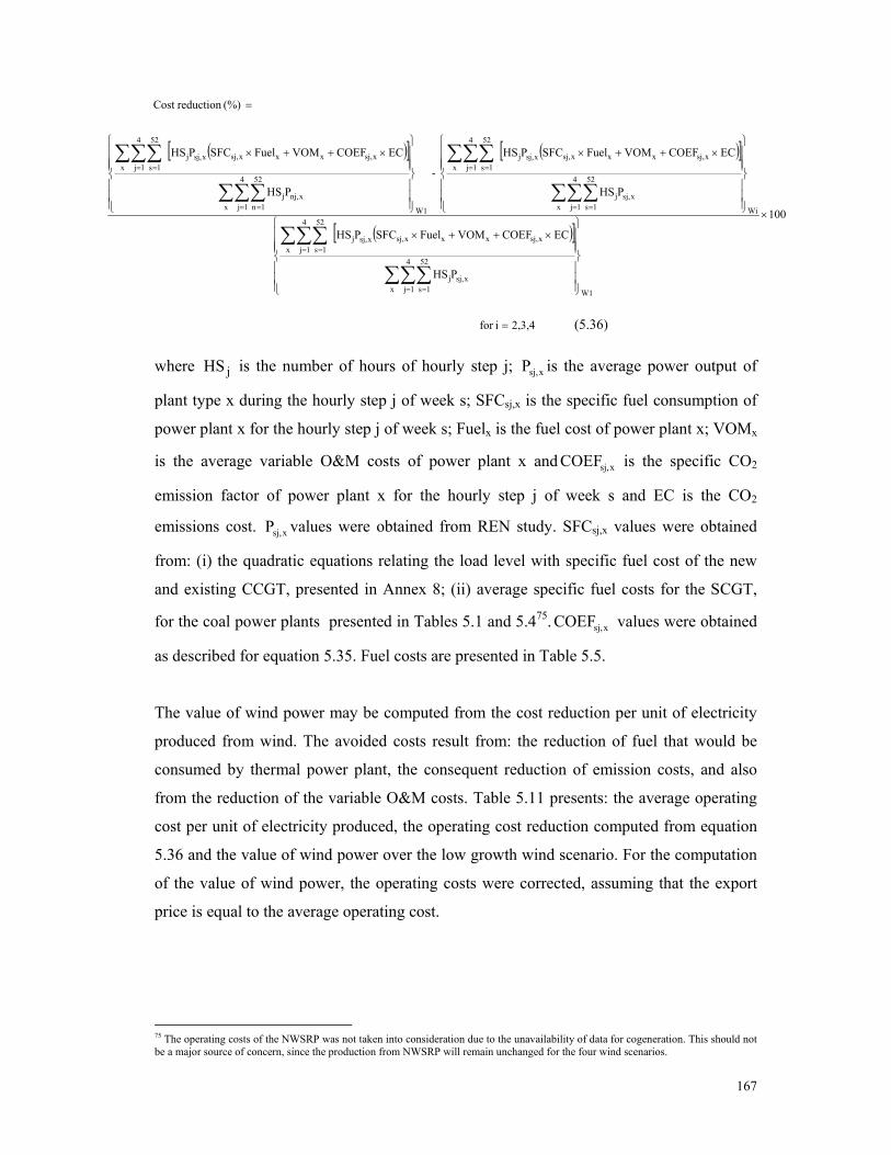
167

( )[ ] ( )[ ]

( )[ ]

(5.36) 2,3,4ifor

100

PHS

ECCOEFVOMFuelSFCPHS

PHS

ECCOEFVOMFuelSFCPHS

-

PHS

ECCOEFVOMFuelSFCPHS

(%)reduction Cost

W1x

4

1j

52

1sxsj,j

xsj,xxxsj,xsj,jx

4

1j

52

1s

Wix

4

1j

52

1sxsj,j

xsj,xxxsj,xsj,jx

4

1j

52

1s

W1x

4

1j

52

1nxnj,j

xsj,xxxsj,xsj,jx

4

1j

52

1s

=

×

⎪⎪⎪

⎭

⎪⎪⎪

⎬

⎫

⎪⎪⎪

⎩

⎪⎪⎪

⎨

⎧×++×

⎪⎪⎪

⎭

⎪⎪⎪

⎬

⎫

⎪⎪⎪

⎩

⎪⎪⎪

⎨

⎧×++×

⎪⎪⎪

⎭

⎪⎪⎪

⎬

⎫

⎪⎪⎪

⎩

⎪⎪⎪

⎨

⎧×++×

=

∑∑∑

∑∑∑

∑∑∑

∑∑∑

∑∑∑

∑∑∑

= =

= =

= =

= =

= =

= =

where jHS is the number of hours of hourly step j; xsj,P is the average power output of

plant type x during the hourly step j of week s; SFCsj,x is the specific fuel consumption of

power plant x for the hourly step j of week s; Fuelx is the fuel cost of power plant x; VOMx

is the average variable O&M costs of power plant x and xsj,COEF is the specific CO2

emission factor of power plant x for the hourly step j of week s and EC is the CO2

emissions cost. xsj,P values were obtained from REN study. SFCsj,x values were obtained

from: (i) the quadratic equations relating the load level with specific fuel cost of the new

and existing CCGT, presented in Annex 8; (ii) average specific fuel costs for the SCGT,

for the coal power plants presented in Tables 5.1 and 5.475. xsj,COEF values were obtained

as described for equation 5.35. Fuel costs are presented in Table 5.5.

The value of wind power may be computed from the cost reduction per unit of electricity

produced from wind. The avoided costs result from: the reduction of fuel that would be

consumed by thermal power plant, the consequent reduction of emission costs, and also

from the reduction of the variable O&M costs. Table 5.11 presents: the average operating

cost per unit of electricity produced, the operating cost reduction computed from equation

5.36 and the value of wind power over the low growth wind scenario. For the computation

of the value of wind power, the operating costs were corrected, assuming that the export

price is equal to the average operating cost.

75 The operating costs of the NWSRP was not taken into consideration due to the unavailability of data for cogeneration. This should not be a major source of concern, since the production from NWSRP will remain unchanged for the four wind scenarios.

168

Table 5.11- Value of wind power over the low growth wind scenario for 2016. Wind scenario

(MW) Average operating cost

(€/MWh) Operating cost reduction (%)

Value of wind power (€/MWhw)1

2000 26.9 -- -- 3500 24.9 7.6% 34.7 4750 23.3 13.5% 34.9 7700 19.6 27.2% 36.5

1 MWhw- electricity produced from wind

According to the results, the electricity production cost reduces almost linearly with the

increasing wind power capacity. Also, the value of wind power increases as wind power

penetration gets higher. Once more, the economic gains obtained with the reduction of

fossil fuel consumption still compensate the loss of efficiency of thermal power plants,

even for large wind power scenarios.

The value of wind power over the low growth wind scenario was also computed assuming

average SFC and average COEF for the CCGT power plants independent of the load level

(values drawn from Tables 5.1 and 5.4). The obtained values ranged between 37.9 €/MWh

and 38.8 €/MWh, indicating once more that using average values leads to the

overestimation of the value of wind power in comparison to values obtained using load

dependent efficiency curves.

V.6.1.5 Comparison of the results with other studies.

Previous works have already addressed the impact that increasing wind power levels may

have on the operating conditions of an electricity system. The ESB National Grid (2004)

study focused on this issue for the Irish electricity system and analysed the impact of the

increasing number of start-ups and of the lower capacity factor of the conventional plants,

as the wind power increases. The Holttinen and Pederson (2003) and Holttinen and

Tuhkanen (2004) studies analysed the effect of large scale wind power on thermal power

system operation and electricity exchanges in the Nordic electricity market.

The results obtained for the Portuguese system, indicate that the increasing of the wind

power electricity production would lead to a significant increase of the electricity exports

to Spain. However, the net exchange increases at a much lower rate than the wind power

electricity generation, as may be seen in Figure 5.10. Thus, in contrast to the Holttinen and

Pederson (2003) study for West Denmark, the major part of the wind power production

169

will not flow abroad and will be used to meet internal consumption.

The Holttinen and Pederson (2003) results for West Denmark and the Rosen et al. (2007)

results for Germany, indicated that the CO2 abatement would be reduced as wind power

penetration gets higher. The different configuration of the Portuguese system justifies part

of the somewhat different values obtained for Portugal. The Danish and German studies

concluded that wind power would mainly replace coal and only in a latter stage would

replace more efficient CCGT units. However, REN study information indicates that in

Portugal wind power will mainly replace CCGT electricity production and, coal power

plants production will only be affected in case of large wind power scenarios. In addition,

increasing wind power leads to higher electricity exports, the amount of electricity

generated by wind plants will not replace the same amount produced by thermal power

plants and there will be an increase of the total electricity production. This fact offsets the

possible reduction of the load level of CCGT and consequent loss of efficiency. Holttinen

and Peddersen (2003) already highlighted this and concluded that when the transmission

possibility was included, the CO2 reductions were very modest when compared with the no

transmission scenarios due to the added exports. These authors argue that the CO2

abatement of wind power in an area that is part of a larger system is especially difficult to

estimate.

The CO2 abatement potential on the Portuguese electricity system seems to be lower than

in the Irish case76. However, for the Portuguese situation this abatement is computed

against the low wind scenario while in the Irish case the abatement is computed against the

non wind case. Higher CO2 reduction values were also obtained for Nordic countries cases

(Holttinen and Tuhkanen, 2004). The authors concluded that wind power increase would

replace mainly electricity generated by coal fired plants, resulting in a CO2 abatement

potential close to 0.7 ton/MWh for both the Nordic and Finish system. However, when

assuming that coal condensing power was no longer used in Finland, new wind power

would replace mainly CCGT capacity reducing significantly the CO2 abatement potential

to less than 0.3 ton/MWh. As for the German system the estimated CO2 abatement

potential ranged between 0.69 ton/MWh and 0.37 ton/MWh (Rosen et al. 2007). According

to the authors, the ecological benefits decreased with the growing share of wind power not

76 ESB National Grid (2004) results indicate that the CO2 abatement potential of wind power generation would reach 0.321 ton/MWhw for 20% wind energy penetration.

170

only due to the reduced fuel efficiency, but also because wind energy substituted CO2-free

electricity production from nuclear power plants.

As with the CO2 abatement case, the value of wind power in Portugal shows an increasing

trend with increasing wind power shares. Once more these results are different from the

ones obtained in Holttinen and Pedersen (2003) and Rosen et al. (2007) studies, who

observed important reductions on the value of wind power as wind penetration gets higher.

However, the Holttinen and Pedersen (2003) results also indicate that for high transmission

scenarios the decrease of the value of wind power was much smaller.

In general, the wind power value of the Portuguese electricity system seems to be higher

than the values obtained in other European studies. Holttinen and Pedersen (2003),

concluded that the value of wind power for West Denmark when operating with out

exchanges laid between 19 and 15 €/MWhw (between 10 and 40% wind penetration). For

the German system, Rosen et al. (2007) estimated that the value of wind power could reach

values between 14 and 11€/MWhw. As wind power is Portugal is expected to replace

mainly CCGT electricity production, the emission gains may not be as high as the ones

reported for these studies where coal electricity production is the most affected, but the

obtained cost savings are higher reflecting the high natural gas prices verified in 2005.

Finally, it should be underlined that the results are strongly affected by the transmission

possibility. Energy exchanges with Spain allow for levelling out the variations in

electricity production, so that the thermal power plants operating regime is not affected as

much by wind power as it would have been without transmission. In fact, if the

transmission possibility was ruled out or significantly reduced, a reduction of the thermal

power output can be expected, which would affect both the load level and the number of

operating hours.

V.6.2 Model formulation

A new planning model was designed to include the impact of wind power on the operating

performance of the thermal power plants. This new model follows the same structure of the

linear EPM described in previous sections. The only differences lay in the cost and

171

emission objective functions, where the gas cost and specific emission factors for the

CCGT will no longer be parameters but rather auxiliary variables depending on the

installed wind power. The constraints will be set equal to the ones described in section

V.3.4.

According to the analysis previously conducted in Section V.6.1, for the inclusion of new

functions relating specific fuel consumption and the CO2 emission factor of the CCGT,

some underlying assumptions had to be considered, namely:

The model deals with the CCGT system and not with individual power plants.

Thus, the individual performance and operating regime of each power plant are not

taken into consideration. Only two subsystems are considered: the existing CCGT

and the new CCGT, each one described by average curves defined by equations

5.31-5.34

If only average functions were used to describe the CCGT subsystem, the model

would be implicitly assuming that all groups would be operating at the same load

level in each moment and this load would remain constant during each interval of

the planning period (month). In reality, there is a merit order ranking different

technologies and power plants and their load will vary during each interval. For

setting the dispatch and managing real time load balancing, the manager of the

system defines the load assigned to each power plant according to a list of operating

parameters that characterise the plants available for dispatch, namely, minimum and

maximum capacity, heat rate curve, start up costs, start up time, amongst others77.

In order to tackle this problem, the model assumes a theoretical distribution of the

load for the CCGT system during the planning period, as follows78:

• each CCGT subsystems will be operating at average load levels

(characterised by equations 5.31-5.34) to produce 50% of their electricity

supply during each interval of the planning period;

• each CCGT subsystems will be operating at a load level 10% higher than

the average to produce 25% of their electricity supply during each interval

of the planning period;

77 The short term planning process is described in detail in Mazer et al. (2007). 78 The problem of assuming load distribution instead of using average functions is longer debated in Annex 9.

172

• each CCGT subsystems will be operating at a load level 10% lower than the

average to produce the remaining 25% of their electricity supply during

each interval of the planning period;

The extent of the impact of the installed wind power on the CCGT load level is

based on data obtained from the theoretical REN study for a set of CCGT’s

operating in the system in 2016 and described by equation 5.30. This study’s

assumptions are, of course part of the base pre-requisites of the optimisation model:

• The study theoretically assumes that different wind scenarios do not

influence the installed power of the remaining system. The study is then

based on a fixed hydro and thermal power system combined with different

wind power scenarios.

• REN study includes the possibility of electricity exports to Spain. However,

the aim of the optimisation model is the search for an optimal electricity

plan to meet internal demand and, as such, the electricity exports are not

accounted for in the optimisation process. By integrating equation 5.30 in

the optimisation model, it is implicitly assumed that for each optimal power

plan obtained, it will be possible to achieve the conditions set under REN

study. If in reality the exports are lower than the estimated values, a sharper

reduction of the average load level of the power plants could be expected

along with a reduction of the number of operating hours. Under those

conditions, there might be some underestimation of the wind power impacts

on the operating performance of the thermal power system.

The optimisation model presupposes that a quadratic function can describe the

characteristic curve of a CCGT. It is also assumed that the characteristic curve of a

CCGT operating in the Iberian market can represent the general shape of the

characteristic curves of the CCGT subsystems considered in the model and

described in equations 5.31-5.34.

The basic assumptions of the linear EPM, described in section V.3.5, are also valid for this

new model. In particular, the model does not deal with specific power plants but with

technologies and no compensation payments are foreseen for reserve power plants.

173

Based on all these assumptions a Non Linear Electricity Planning Model (NLEPM) was

obtained and is described in the next sections.

V.6.2.1 Cost objective

According to equations 5.31-5.34 and the assumed load distribution, the specific fuel

consumption and CO2 emission factor for the existing and candidate CCGT subsystems

will be computed from equations 5.37 to 5.48.

25%79

( ) ( ) ( )( ) ( ) ( ) (5.38) 0.355IPIPIP 101.02IPIPIP 102.41COEF

(5.37) 162.6IPIPIP 10 4.66IPIPIP 101.10 SFC

t3b,t3a,9t6-2

t3b,t3a,9t9-

a5t

t3b,t3a,9t-42

t3b,t3a,9t-6

a5t

+++×+++×=

+++×+++×=


(5.39) 152.8IPIPIP 104.38IPIPIP 101.04 SFC

t3b,t3a,9t7-2

t3b,t3a,9t9-

a2t

t3b,t3a,9t-42

t3b,t3a,9t-6

a2t

+++×+++×=

+++×+++×=

50%80



t3b,t3a,9t6-2

t3b,t3a,9t9-

b5t

t3b,t3a,9t-32

t3b,t3a,9t-6

b5t

+++×−++×=

+++×−++×=



t3b,t3a,9t6-2

t3b,t3a,9t9-

b2t

t3b,t3a,9t-32

t3b,t3a,9t-6

b2t

+++×−++×=

+++×−++×=

25%81



t3b,t3a,9t5-2

t3b,t3a,9t9-

c5t

t3b,t3a,9t-32

t3b,t3a,9t-6

c5t

+++×−++×=

+++×−++×=



t3b,t3a,9t5-2

t3b,t3a,9t9-

c2t

t3b,t3a,9t-32

t3b,t3a,9t-6

c2t

+++×−++×=

+++×−++×=

Where: (SCF5t)a Specific gas consumption for generating 25% of electricity supplied by existing CCGT in

each month of year t (m3N/MWh).

(SCF5t)b Specific gas consumption for generating 50% of electricity supplied by existing CCGT in


79 In each month of year t, 25% of the electricity produced on the existing CCGT brings about a SFC drawn from equation 5.37 and a CO2 emission factor drawn from equation 5.38.The same way, 25% of the electricity produced on the new CCGT brings about a SFC drawn from equation 5.39 and a CO2 emission factor drawn from equation 5.40. 80 In each month of year t, 50% of the electricity produced on the existing CCGT brings about a SFC drawn from equation 5.41 and a CO2 emission factor drawn from equation 5.42.The same way, 50% of the electricity produced on the new CCGT brings about a SFC drawn from equation 5.43 and a CO2 emission factor drawn from equation 5.44. 81 In each month of year t, 25% of the electricity produced on the existing CCGT brings about a SFC drawn from equation 5.45 and a CO2 emission factor drawn from equation 5.46.The same way, 25% of the electricity produced on the new CCGT brings about a SFC drawn from equation 5.47 and a CO2 emission factor drawn from equation 5.48.

174

(SCF5t)c Specific gas consumption for generating the remaining 25% of electricity supplied by

existing CCGT in each month of year t (m3N/MWh).

(SCF2t)a Specific gas consumption for generating 25% of electricity supplied by candidate CCGT in


(SCF2t)b Specific gas consumption for generating 50% of electricity supplied by candidate CCGT in


(SCF2t)c Specific gas consumption for generating the remaining 25% of electricity supplied by

candidate CCGT in each month of year t (m3N/MWh).

(COEF5t)a CO2 emission factor for generating 25% of electricity supplied by existing CCGT in each

month of year t (ton/MWh).

(COEF5t)b CO2 emission factor for generating 50% of electricity supplied by existing CCGT in each


(COEF5t)c CO2 emission factor for generating the remaining 25% of electricity supplied by existing


(COEF2t)a CO2 emission factor for generating 25% of electricity supplied by candidate CCGT in each


(COEF2t)b CO2 emission factor for generating 50% of electricity supplied by candidate CCGT in each


(COEF2t)c CO2 emission factor for generating the remaining 25% of electricity supplied by candidate


Combining these equations with equation 5.4 the total variable cost for the NLEPM may

now be obtained from equation 5.49.

( ) ( )[ ]

( ) ( )[ ]

( ) ( ) ( ) ( )( ) ( ) ( ) ( )( ) ( ) ( ) ( )

( )

( ) ( ) ( ) ( )( ) ( ) ( ) ( )( ) ( ) ( ) ( )

( ) (5.49) i1∆0.25PCOEFEC0.25PGCSFC

0.5PCOEFEC0.5PGCSFC0.25PCOEFEC0.25PGCSFCPVOM

(€) i1∆0.25PCOEFEC0.25PGCSFC


i1∆PCOEFECFVOM

i1∆PCOEFECFVOMVC

h

th

5htc5t5htc5t

5htb5t5htb5t

5hta5t5hta5t5ht5

t

h

th

2htc2t2htc2t

2htb2t2htb2t

2hta2t2hta2t2ht2

t

t h 5l

thlhtlll

t h 2k

thkhtkkk

∑∑

∑∑

∑∑∑

∑∑∑

⎪⎭

⎪⎬

⎫

⎪⎩

⎪⎨

⎧

+×⎥⎥⎥

⎦

⎤

⎢⎢⎢

⎣

⎡

××+××

+××+××

+××+××+×

+

⎪⎭

⎪⎬

⎫

⎪⎩

⎪⎨

⎧

+×⎥⎥⎥

⎦

⎤

⎢⎢⎢

⎣

⎡

××+××

+××+××

+××+××+×

+

+××××+++

+××××++=

−

−

≠

−

≠

−

Where GC is a parameter for the natural gas cost (€/m3N). This value may be found in

175

Table 5.5, summarising the general assumptions under the base scenario. The first two

terms of the equation are linear and represent the total variable cost of power plants

excluding CCGT. The last two terms of the equation are non linear and represent the total

variable cost of the CCGT.

The fixed cost will be obtained from equation 5.3 and the total cost equation may be

described according to equation 5.50.

( )

( ) ( )[ ]

( ) ( )[ ]

( ) ( ) ( ) ( )( ) ( ) ( ) ( )( ) ( ) ( ) ( )

( )

( ) ( ) ( ) ( )( ) ( ) ( ) ( )( ) ( ) ( ) ( )

( ) (5.50) i1∆0.25PCOEFEC0.25PGCSFC


(€) i1∆0.25PCOEFEC0.25PGCSFC


i1∆PCOEFECFVOM

i1∆PCOEFECFVOM

i1 IPFOM1i)(1

i)i(1IC

h

th

5htc5t5htc5t

5htb5t5htb5t

5hta5t5hta5t5ht5

t

h

th

2htc2t2htc2t

2htb2t2htb2t

2hta2t2hta2t2ht2

t

t h 5l

thlhtlll

t h 2k

thkhtkkk

t k

tktknk

nk

k

∑∑

∑∑

∑∑∑

∑∑∑

∑∑

⎪⎭

⎪⎬

⎫

⎪⎩

⎪⎨

⎧

+×⎥⎥⎥

⎦

⎤

⎢⎢⎢

⎣

⎡

××+××

+××+××

+××+××+×

+

⎪⎭

⎪⎬

⎫

⎪⎩

⎪⎨

⎧

+×⎥⎥⎥

⎦

⎤

⎢⎢⎢

⎣

⎡

××+××

+××+××

+××+××+×

+

+××××+++

+××××+++

⎭⎬⎫

⎩⎨⎧

+×⎥⎦

⎤⎢⎣

⎡+

−++

=

−

−

≠

−

≠

−

−

The final value obtained from this equation, corresponds to total cost of the electricity

system for a 10 years planning period, taking into consideration the impact of wind power

on the CCGT operating performance.

V.6.2.2 Emissions objective

The specific CO2 emission factor for the CCGT will be computed from equation 5.38, 5.42

and 5.46 for the existing power plants and from equation 5.40, 5.44 and 4.48 for the

candidate power plants. Combining these equations with equation 5.6, the total CO2

emissions may be obtained:

176

( )[ ] ( )[ ]

( ) ( ) ( ) ( ) ( ) ( )[ ]{ }

( ) ( ) ( ) ( ) ( ) ( )[ ]{ } (5.51) ∆0.25PCOEF0.5PCOEF0.25PaCOEF

(ton) ∆0.25PCOEF0.5PCOEF0.25PCOEF

∆PCOEF ∆PCOEFCO

hh5htc5t5htb5t5ht5t

t

hh2htc2t2htb2t2hta2t

t

t h 5lhlhtl

t h 2khkhtk

∑∑

∑∑

∑∑∑∑∑∑

×+×+×+

×+×+×+

××+××=≠≠

The first two terms of equation 5.51 are linear and represent the sum of the monthly

emissions released by the power plants during the planning period excluding CCGT. The

last two terms of the equation are non linear and represent the sum of the monthly

emissions released by the CCGT during the planning period. The final value obtained from

this equation corresponds to total CO2 emissions expected to be released during the next 10

years, taking into consideration the impact of wind power on the CCGT operation.

V.6.2.3 Final considerations

Figure 5.11 shows the flow diagram for the NLEPM, including the input information,

output results and the optimisation problem.

Average SFC1

Average COEF2

Coal

Fueloil

SCGT

Mat

hem

atic

al fu

nctio

ns :

SFC

=f(

inst

alle

d w

ind

pow

er)

CO

EF=f

( ins

talle

d w

ind

pow

er)

Installed wind power

SFC1

CCGTCOEF2

Internal calculations of the models


CO2

production

Results

GAMS code


CO2 production


Results

GAMS code

Cost

CO

Linear objectives

Demand

Legal

System

Linear constraints

Plant

Load

Cost

2

Non linear objective functions

Demand

Legal

System

Linear constraints

Plant

Load

Data


Cost

Average SFC1

Average COEF2

Coal

Fueloil

SCGT

Average SFC1

Average COEF2

Coal

Fueloil

SCGT

Average SFC1

Average COEF2

Coal

Fueloil

SCGT

Mat

hem

atic

al fu

nctio

ns :

SFC

=f(

inst

alle

d w

ind

pow

er)

CO

EF=f

( ins

talle

d w

ind

pow

er)


SFC1

CCGTCOEF2



SFC1

CCGTCOEF2


SFC1

CCGTCOEF2

SFC1

CCGTCOEF2



CO2

production

Results

GAMS code


CO2 production


Results

GAMS code

Cost

CO

Linear objectives

Demand

Legal

System

Linear constraints

Plant

Load

Cost

2

Non linear objective functions

Demand

Legal

System

Linear constraints

Plant

Load

Data


Cost

Figure 5.11- Non linear electricity planning model.

As with the EPM the input information for the problem includes the mathematical

formulation of the objective functions and of the constraints. However, now the cost and

177

CO2 objective functions are no longer linear. The input data still describes the technical

and economic characteristics of the present and candidate power plants and the expected

load pattern. This non linear model also assumes average specific fuel consumption and

CO2 emission factors for coal power plants, fueoil power plants and SCGT. The specific

fuel consumption and CO2 emission factors for the CCGT system are now based on

empirical data and are described by quadratic functions relating these variables with the

installed wind power.

V.6.3 NLEPM results

As the EPM, the NLEPM was written in a GAMS code and the Branch and Bound

algorithm was used, calling BARON solver in order to ensure a global optimum for the

problem. However, the dimension and complexity of the model led to some difficulties in

the convergence process which was reflected mainly in the execution time. Karuppiah and

Grossmann (2006) and Murray and Shanbhag (2007), already reported similar difficulties

with BARON, such that to guarantee a global optimum for large problems this would

mostly be reflected in the amount of computational time. As Bussieck et al. (2003) stated

“.. an higher solution quality is often obtained at a cost of efficiency. Thus, users should

consider if feasibility of the (local) solution and efficiency or global optimality at a cost of

efficiency is the primary criteria.”

To overcome these difficulties, BARON was used as a first approach to the problem,

imposing a time limit and a maximum optimal tolerance of 0.025. Subsequently, local

solver Standard Branch and Bound (SBB) was called upon to work out the problem,

imposing zero optimal tolerance and setting the upper bound of the objective function

equal to the value obtained with BARON optimisation. This ensures that the local solver is

converging to the global optimum of the problem, and reduces significantly the necessary

time to solve the problem.

SBB is a commercially available solver from Akri Software (SBB, no date). Some recent

examples of studies using this solver include the optimisation of the energy management of

a large-scale water supply network (Bounds et al. 2006), the optimisation of power

production of small-scale CHP plants (Savola and Fogelholm, 2007) or the ECO-optimised

reuse of processed liquors (Erol and Thoming, 2005).

178

Figure 5.12 represents the computational approach to the optimisation process.

Minimisation using BARON

OptCr ≤2.5%

Stopping criteria

Minimisation using SBB

OptCr =0%

Stopping criteria

Final solution

First solution

Minimisation using BARON

OptCr ≤2.5%

Stopping criteria

Minimisation using SBB

OptCr =0%

Stopping criteria

Final solution

First solution

Figure 5.12- Computational approach to the optimisation process.

According to the above, the approach to the NLEPM will involve the following main

stages:

(1) Minimisation of the CO2 objective, using BARON and SBB solvers.

(2) Minimisation of the cost objective, using BARON and SBB solvers.

(3) Definition of CO2 allowable levels between (1) and CO2 values obtained with

the minimisation of the cost objective (2).

(4) Minimisation of the cost objective constrained by the CO2 allowable levels,

using BARON and SBB solver.

(5) Construction of the final set of optimal solutions.

The GAMS code for the NLEPM solver may be found in Annex 10.

The process started again with the optimisation of each one of the objectives separately

over the set of constrains. The final results of these individual optimisations are shown in

table 5.12. The first solutions found with BARON solver are reported in Annex 11. Table 5.12- Results of the single objective optimisation for the NLEPM.

Absolute values Unit values Cost (M€) CO2 (Mton) Cost (€/MWh) CO2 (ton/MWh)

Optimal cost solution (NLS0) 16621 310.8 31.537 0.590 Optimal CO2 solution (NLS8) 23338 134.7 44.283 0.256

The elements in the first row indicate that the least costly solution (31.5 €/MWh)

corresponds to an average value for the CO2 emissions of 0.590 ton/MWh. The elements in

the second row indicate that the least polluting solution (0.256 ton/MWh) corresponds to

an average cost of about 44.3 €/MWh. This means that the least costly solution is 29% less

179

expensive than the solution with the lowest emission levels. In addition, it should be noted

that the corresponding emission levels are more than twice the ones obtained with the

lowest CO2 solution. Comparing these results to the ones obtained with the linear EPM, it

is clear that reduction of the CO2 emissions as a consequence of the wind power impact on

the operating performance of the CCGT plants can only be achieved with increased

economic effort. The NLEPM never reaches CO2 emission levels as low as the EPM for

the assumed electricity demand conditions, while the minimal CO2 values are about 30%

higher in the NLEPM than in the linear model.

As with the EPM, the process continued with the bi-objective optimisation, with each one

of the objectives limited by the previously identified extreme values. Once more,

optimisation BARON solver was used to solve the problem, with the relative optimal

tolerance (Optcr) set equal to 2.5%. Hereafter the local solver SBB was called upon to

work out the problem, imposing zero optimal tolerance. The process was repeated for each

run conducted.

Table 5.13 presents the final data sets from this optimisation process. The elements in the

second column represent the absolute optimal cost solution constrained by the CO2 level

indicated in the third column. The fourth and fifth columns represent the respective unit

cost and CO2 values. The last column present the run time for each simulation using SBB

solver.

Table 5.13- Results of the two objective optimisation for the NLEPM.

Cost Absolute values Unit values Run time optimisation Cost (M€) CO2 (Mton) Cost (€/MWh) CO2 (ton/MWh) (min)

NLS0 16621 311 31.537 0.590 2.9 NLS1 16882 275 32.033 0.522 8.1NLS2 17149 250 32.539 0.474 7.5 NLS3 17392 225 33.001 0.427 8.3 NLS4 17722 200 33.627 0.379 7.2NLS5 18111 175 34.365 0.332 7.4 NLS6 18640 150 35.369 0.285 7.5 NLS7 20319 138 38.554 0.262 1.8NLS8 23338 135 44.283 0.256 0.02

All the models were formulated using GAMS and solved on a Intel Core Due, 987 MHz

computer with 1GB memory. The first solutions found with BARON solver may be seen in

Annex 11.

180

Figure 5.13 graphically represents the set of optimal solutions, corresponding to the

average cost vs. CO2 trade-off. The two extreme points of the line obtained correspond to

the extreme solutions presented in Table 5.12.

0.0

0.1

0.2

0.3

0.4

0.5

0.6

0.7

31 33 35 37 39 41 43 45

Cost (€/MWh)

CO

2 (t/

MW

h)


Opt

imal

CO

2 so

lutio

n

NLS1

NLS2

NLS3

NLS4

NLS5

NLS6NLS7

NLS0

NLS8

Figure 5.13- Pareto curve solutions for the NLEPM.

Table 5.14 describes the power generation expansion planning for these optimal solutions.

Table 5.14- Incremental installed power (MW) for the optimal solutions for the NLEPM.

2008 2009 2010 2011 2012 2013 2014 2015 2016 2017 Total Coal 1950 300 750 450 750 300 4500

NLS0 Gas 330 330 Wind 941 813 15 64 744 0 1271 3848 Coal 300 900 300 1500 0 600 300 3900

NLS1 Gas 400 400 800 Wind 1414 277 39 467 293 154 1769 4413 Coal 300 1000 450 600 450 2800

NLS2 Gas 660 330 330 660 330 2310 Wind 331 102 628 494 62 433 744 154 277 3225 Coal 300 600 900

NLS3 Gas 660 330 330 660 330 990 400 330 4030 Wind 320 107 697 431 74 335 135 23 827 634 3583 Coal

NLS4 Gas 400 400 330 730 330 1200 330 330 330 660 5040 Wind 1414 146 517 141 543 464 3225 Coal

NLS5 Gas 400 400 400 800 330 1390 730 660 5110 Wind 1414 54 598 771 388 3225 Coal

NLS6 Gas 2000 400 400 400 400 330 400 330 330 4990 Wind 1118 349 255 144 16 183 329 425 431 3250 Coal

NLS7 Gas 3390 400 330 330 330 330 660 400 660 6830 Wind 4569 4569 Coal 0

NLS8 Gas 3630 0 660 660 0 330 330 330 660 330 6930 Wind 7500 7500

181

Table 5.15 presents the corresponding final configuration of the electricity system in 2017,

described by the total installed power for each technology and by the respective

contribution for electricity supply.

Table 5.15- Configuration of the electricity system in 2017 for the optimal solution.

NLS0 NLS1 NLS2 NLS3 NLS4 NLS5 NLS6 NLS7 NLS8

Tota

l in

stal

led

pow

er

(MW

)

Coal (new) 4500 3900 2800 900 Coal (existing) 1820 1820 1820 1820 1820 1820 1820 1820 1820 Gas (new) 330 800 2310 4030 5040 5110 4990 6830 6930 Gas (existing) 2916* 2916* 2916* 2916* 2916* 2916* 2916* 2916* 2916*Wind (new) 3848 4413 3225 3583 3225 3225 3250 4569 7500 Wind (existing) 1515 1515 1515 1515 1515 1515 1515 1515 1515 Large hydro 5805 5805 5805 5805 5805 5805 5805 5805 5805NWSRP(1) 3245 3245 3245 3245 3245 3245 3245 3245 3245 Total 23979 24414 23636 23814 23566 23636 23541 26700 29731

Con

tribu

tion

to

elec

trici

ty su

pply

(%) Coal (new) 44 38 27 8 0 0 0 0 0

Coal (existing) 13 15 11 18 10 0 0 0 0 Gas (new) 3 5 21 33 49 49 48 59 51 Gas (existing) 1 1 1 1 1 11 12 0 0 Wind 14 16 13 14 13 13 13 16 24 Large hydro 14 14 16 15 16 16 16 14 14 NWSRP 11 11 11 11 11 11 11 11 11 Total 100 100 100 100 100 100 100 100 100

Share of RES (%)(2) 39 40 39 39 39 39 39 40 49 External dependency (%) (3) 65 64 65 65 65 65 65 63 55 2017 electricity demand 85951 GWh


From these results it can be concluded that the least costly solution assumes investments

mainly in new coal power plants. New wind power appears only after 2010 due to the

renewable constraint. According to this solution, in 2017:

The electricity supply would come mainly from new and old coal power plants.

CCGT would also be operating but representing only about 4% of the electricity

supply.

The remaining electricity would come from non large thermal power stations


11%).

The electricity consumption from renewable energy sources would represent 39 %

182

of the total electricity demand (meeting but not exceeding the renewable

Directive).


energy sources (mainly coal).

The results are not much different from the ones obtained with the EPM. Both the

costs and CO2 values are close to the ones obtained with the linear model and so

are the proposed investment strategies.

The lowest CO2 emission solution represents a completely different scenario. It assumes

the complete disinvestment in coal, and a significant investment in CCGT and renewable

energy sources, maximising the use of wind. According to this solution, in 2017:

The electricity supply would come mainly from new gas power plants.

Old coal power plants would not operate and no new coal plants would be added to

the system.

The remaining electricity would come from non large thermal power stations


11%).

The electricity consumption from renewable energy sources would represent 49%

of the total consumption (outreaching the renewable Directive).


energy sources (natural gas).

In spite of the estimated wind power impact on the CCGT operating performance,

the investment strategy is also close to the one obtained with the EPM. In fact, the

minimisation of CO2 emissions may only be achieved by the maximisation of

electricity generation from wind power combined with clean thermal power plants

like CCGT.

183

The costs and CO2 values are now higher than the ones obtained with the linear

model. The integration into the model of the estimated impact of wind power in

CCGT operating performance resulted in almost 14% cost increase and also in a

30% CO2 emissions increase in comparison with the EPM results.

The initial effect of imposing increasing CO2 constraints on the model is a reduction of the

investment in new coal power plants, combined with the increase of investment in new

onshore wind power plants and a small increase of investment in new CCGT. For solution

NLS1, the least costly way to achieve the imposed CO2 levels is still relying mainly on

coal power production but investments in new wind power plants are required in order to

offset the CO2 emissions.

Solutions NLS2 and NLS3 present both a reduction on installed coal and wind power

comparatively to NLS1. The integration of new CCGT into the system compensates this

reduction and ensures the imposed CO2 limits. Solution NLS4 proposes no more

investments on new coal but electricity generation from existing coal power plants still

represents 10% of the total electricity supplied. Solutions NLS5 and NL6 represent already

highly environmentally constrained solutions. Both these solutions present close strategies,

where the reduction of the CO2 levels is mainly achieved by the full replacement of the

coal power production by the natural gas power production. The installed wind power will

only present a more significant increase when very low CO2 limits are imposed to the

model, as in solution NLS7.

For solutions NLS2-NLS6, the share of electricity generated for RES is equal to 39%, a

value just enough to meet the minimal goal imposed by renewable Directive 2001/77/EC

for Portugal. Solutions NLS1 and NLS7 surpass this minimal request, due to their higher

total installed wind power. The level of wind power in the system also strongly influences

the value of the external dependency, assigned to each solution. The results of the NLEPM

indicate that solutions NLS1 and NLS7 not only present higher RES share but also

contribute to the reduction of the external energy dependency.

It should however be underlined that the optimisation procedure aims to reduce a very

large number of possible plans, to a small number of plans that are to be presented to the

decision makers. Due to the uncertainties associated with the calculations it may not be

184

easy to discard some possible plan that although not being optimal is not significantly

worse than another mathematical optimal plan (Hobbs and Meier, 2003). As seen, cost and

CO2 tradeoff analysis leave aside important aspects like the external dependency or the

need to diversify the fuel mix of the country. It is worth then to analyse some other

solutions that are not located in the Pareto front but may bring some additional advantages

to the system with out seriously compromising cost or CO2 objectives.

V.6.3.1 Non optimal solutions of NLEPM

For obtaining non optimal example solutions for the model, sensitivity runs for solutions

NLS3, NLS4 and NLS5 were conducted. For this it was assumed that additional

constraints were added to the model, imposing minimum predefined installed wind power

levels for the future. The model was run again and new solutions were obtained,

corresponding to the same CO2 level but with higher costs and consequently moving away

from the original Pareto front.

As an example, it was assumed that the decision maker adds an additional constraint,

imposing that the new installed wind power in 2012 must reach at least 6500 MW, as

indicated in equation 5.52.

6500IP3a,2012 ≥ (5.52)

Table 5.16 summarises the results of this sensitivity exercise for three examples (NLS3,

NLS4 and NLS5). The final configuration of the electricity system in 2017 along with

expected average cost and CO2 emissions, for the original Pareto solutions and for the ones

obtained after imposing additional constraints to the model are presented.

The results indicate that imposing values for installed wind power beyond the original

optimal solutions would affect the operating conditions of the system and the share of

electricity supplied by each technology. In general, the electricity production from CCGT

would be reduced but the share of electricity produced from both coal and wind power

would increase. This new impositions lead to higher costs but, at the same time, contribute

to the reduction of the external dependency and to the increase of the share of electricity

produced from RES.

185

Table 5.16- Results for the original Pareto and additionally constrained solutions in 2017 NLS3 NLS3.1 NLS4 NLS4.1 NLS5 NLS5.1

Observations Pareto IP3a,2012≥6500 Pareto IP3a,2012≥6500 Pareto IP3a,2012≥6700

Tota

l in

stal

led

pow

er

(MW

)

Coal (new) 900 2700 2400 600 Coal (existing) 1820 1820 1820 1820 1820 1820 Natural gas (new) 4030 1650 5040 1860 5110 3720 Natural gas (existing) 2916* 2916* 2916 2916* 2916* 2916* Wind (new) 3583 6500 3225 6514 3225 6500 Wind (existing) 1515 1515 1515 1515 1515 1515 Large hydro 5805 5805 5805 5805 5805 5805 NWSRP 3245 3245 3245 3245 3245 3245 Total 23814 26151 23566 26075 23636 26121

Con

tribu

tion

to

elec

trici

ty su

pply

(%) Coal (new) 8 26 0 23 0 5

Coal (existing) 18 5 10 11 0 7 Natural gas (new) 33 16 49 18 49 36 Natural gas (existing) 1 6 1 2 11 4 Wind 14 22 13 22 13 22 Large hydro 15 14 16 13 16 15 NWSRP 11 11 11 11 11 11 Total 100 100 100 100 100 100

Share of RES (%) 39 46 39 45 39 46 External dependency (%) 65 57 65 58 65 57 Cost (€/MWh) 33.001 33.864 33.627 34.961 34.365 36.950 CO2 (ton/MWh) 0.427 0.427 0.379 0.379 0.332 0.332 2017 electricity demand 85951


For example solution NLS4.1 is 4% more expensive than the original NLS4. However, in

2017 it would be possible to reduce the external dependency of the electricity generation

sector by 7% and the share of RES would increase by 6%, comparatively to the original

values reported under NLS4. Concerning the coal/natural gas balance, NL4.1 represents

also a more equilibrated solution, allowing for the diversification of suppliers of primary

energy thereby increasing the security of supply.

Figure 5.14 graphically represents the set of the original compromise Pareto solutions for

the NLEPM and the new solutions that, although representing trade-offs between the two

objectives, do not belong to the Pareto front of the original NLEPM.

186

0.0

0.1

0.2

0.3

0.4

0.5

0.6

0.7

31 33 35 37 39 41 43 45

Cost (€/MWh)

CO

2 (t/

MW

h) Opt

imal

CO

2 so

lutio

n


NLS4.1NLS5.1

Non-optimal solutions

NLS4

NLS5

NLS3.1

NLS3

Figure 5.14- Original Pareto solutions and additionally constrained solutions.

The aim of this exercise was not to present an exhaustive description of all possible plans,

but rather draw attention to some examples demonstrating the relevance of presenting other

possible strategies that, although not being original Pareto solutions, may be interesting

from the decision maker’s perspective. The three non optimal solutions analysed ensure the

required minimum CO2 levels, set for each run, and present also a cost increase of less than

10% over the optimum solutions. However, they may become more interesting when other

aspects, like the external energy dependency or the need to balance coal and gas in the

system, are considered.

V.6.3.2 Final comments

The results obtained, and in particular the curve presented in Figure 5.13, indicate that the

drop of CO2 emissions per unit of cost falls deeply for highly environmentally constrained

solutions. Between the optimal cost solution and NLS6 the cost per ton of CO2 reduction is

12.6 €. A value obtained mainly due to the high environmental gains achieved with the

substitution of coal power electricity generation by wind and CCGT production. Between

NLS6 and optimal CO2 solution, the ∆cost∆CO2 ratio increases to 307.4 €/ton CO2. For this

range of the curve, the more pollutant plants are not producing any electricity any more

and the environmental gains may only be achieved by the installation of new CCGT and

new wind power plants.

187

The results may be described by four main scenarios:

Scenarios with low CO2 restrictions (NLS1). The cost minimisation with minimal

environmental restrictions is achieved by the combined investment in new coal and

wind power plants. The electricity production comes mainly from existing and new

coal power plants. The onshore wind power production allows for higher electricity

generation from RES and the system exceeds the minimum requirements set by

Directive 2001/77/EC for Portugal Also, this wind power scenario allows for

slightly reducing the external energy dependency to 64%.

Scenarios with moderate CO2 restrictions (NL2, NLS3). Investments in new coal

power plants decline but, on the other hand, investments in new CCGT increase.

However electricity production from coal power plants still represents an important

share of the total electricity supplied. There are also new investments in wind

power plants, although less significant than in NLS1. In 2017, the electricity

consumption from renewable energy sources represents 39% of the total electricity

demand and the share of electricity consumption from imported primary energy

sources is about 65%.

Scenarios with strong CO2 restrictions (NLS4-NL6). The less expensive way to

ensure severe CO2 limitation is the strong investment in new CCGT with electricity

production coming mainly from the new and existing natural gas power plants. The

investment in new wind power plants is slightly lower than in previous solutions. In

2017, the electricity consumption from renewable energy sources represents 39% of

the total demand and, the share of electricity consumption obtained from imported

primary energy sources is about 65%. By limiting the total wind power production,

the model attempts to minimise the effects on CCGT operating performance. Under

these solutions, the thermal power mix relies mainly on natural gas which reduces

the possibility of diversification of primary energy suppliers and makes the

electricity system highly vulnerable to the international prices of natural gas.

Scenarios with extreme CO2 restrictions (NLS7). This extreme condition may

only be achieved by the replacement of the existing CCGT plants by new CCGT

and new wind power plants. In 2017, the share of renewable energy coming from

188

renewable energy sources is more than 40% and the electricity consumption

coming from imported primary energy sources declines to about 63%. As with

solution NLS6, the issues of security of supply and exposure to international natural

gas price fluctuations are important aspects to consider under this solution.

Power system planning is not an exact science and the robustness of the results across

alternative scenarios must be checked. This was done by a sensitivity analysis, where

important parameters of the model were changed and new results were generated. The next

section of this chapter presents the results of this analysis.

V. 6.4 Sensitivity analysis

The increasing uncertainty surrounding the electricity generating sector makes the

sensitivity analysis an essential toll to long term planning. The fuel price volatility and the

emissions trading schemes, probably represent the major sources of uncertainty, since the

economic interest of wind power largely depends on these two factors. In this section, both

these aspects will be analysed. Preliminary investigations on the evolution of the fuel

prices and of the CO2 allowances prices were conducted and some possible future

scenarios were drawn. Whereafter the optimisation was conducted with the NLEPM.

Sensitivity analysis in relation to the discount rate was also carried out, following

IEA/NEA (2005) scenarios.

The sensitivity analysis will focus on two main scenarios: the optimal cost solution,

without environmental restrictions (solution Opt. cost) and the Kyoto reference solution as

described in Section V.5.1, with an average CO2 maximum emission limit equal to 20

Mton/year for the planning period (solution SR1). Additional scenarios were also

considered in some of the sensitivity runs to better illustrate the results of this exercise.

V.6.4.1 Fuel Price

Both the EPM and the NLEPM assume that coal and natural gas prices will remain stable

and at 2005 levels during the 10 years planning period. However, between 1999 and 2005

the fuel prices followed an increasing pattern, as may be observed from Figure 5.15.

189

20

70

120

170

220

1999 2000 2001 2002 2003 2004 2005

Year

Pric

eNatural gas (€/10^3Nm3) Coal (€/t) Fuel oil (€/t)

Figure 5.15 – Average price of fuel purchased by EDP producers (2005 values). Source: EDP (2006b), EDP (2004a), EDP (2002).

The household and industrial consumers’ prices seem to indicate that the natural gas prices

are giving signs of stabilisation in 2006 and beginning of 2007, after the high increase in

the first semester of 2005. The European Commission projections (European Commission,

2006a) indicate that an average annual growth rate of more than 7% may be expected for

gas, between 2000 and 2010. Between 2010 and 2020, this growth rate may be close to

0.9%. For the sensitivity analysis two possible annual average growth rates for natural gas

were analysed: moderate growth rate (4% per year) and high growth rate (7% per year).

Table 5.17 summarises the main results of the sensitivity run for the NLEPM.

According to the results, the natural gas price increase would lead to a stronger investment

in coal power plants and a reduction of gas fired electricity generation. The optimal cost

solution indicates that the wind power capacity remains close to the base scenario, for both

the moderate and high gas increase sensitivity run. In 2017, electricity production would

come mainly from existing and new coal power plants.

For the Kyoto reference scenario (SR1), the model converges to solutions characterised by

strong investments in new coal power plants combined with high installed wind power

capacity (both on and offshore). For the last years of the planning period, natural gas

would become too expensive to compete with coal or wind power electricity production

and the electricity production from CCGT would be kept at minimal levels set by equation

5.25.

190

Table 5.17- Results of the natural gas price sensitivity run for the NLEPM in 2017. Moderate gas price growth rate (4%) High gas price growth rate (7%)

Opt. cost SR1 Opt. cost SR1 To

tal

inst

alle

d po

wer

(M

W)

Coal (new) 4800 4300 4800 4500 Coal (existing) 1820 1821 1820 1821 Natural gas (new) 2190 330 1790 Natural gas (existing) 2916 2916 2916 2916 Wind (new) 4102 7034 4102 7500 Wind (existing) 1515 1515 1515 1515 Large hydro 5805 5805 5805 5805 NWSRP 3245 3245 3245 3245 Total 24203 28826 24533 29092

Con

tribu

tion

to

elec

trici

ty su

pply

(%) Coal (new) 47 40 47 41

Coal (existing) 10 9 10 6 Natural gas (new) 0 3 3 3 Natural gas (existing) 3 0 0 0 Wind 15 23 15 24 Large hydro 14 14 14 15 NWSRP 11 11 11 11 Total 100 100 100 100

Cost (M€) 16878 19502 17069 20223 CO2 (Mton) 316 200 316 200 Cost (€/MWh) 32.026 37.005 32.387 38.373 CO2 (ton/MWh) 0.600 0.379 0.600 0.379 2017 electricity demand 85951 GWh

According to the results, the rising trend of the natural gas price may result in a different

optimal configuration of the electricity system. Even when imposing emission limits, coal

will have an important role in particular in the later years of the planning period.

According to solution SR1, the minimum Kyoto commitments would be achieved mainly

by combining coal power electricity production (especially from new plants) and wind

power generation. For this solution, the average yearly cost increase comparatively to the

base case scenario is close to 3.4 €/MWh for the low gas price growth rate simulation and

4.7 €/MWh for the high gas price growth rate simulation.

However, it is also important to analyse the simultaneous increase of both natural gas and

coal prices. According to the European Commission projections, coal price will also

increase by about 4% per year between 2000 and 2010 and by about 1.2% per year

between 2000 and 2010. Table 5.18 summarises the main results of the sensitivity run

combining an annual growth rate of 4% for natural gas with an annual growth rate 2.6%

for coal.

191

Table 5.18- Results of the natural gas and coal prices sensitivity run for the NLEPM in 2017. Moderate coal and gas prices growth rate

Opt. cost SR1

Tota

l in

stal

led

pow

er

(MW

)

Coal (new) 4800 4200 Coal (existing) 1820 1821 Natural gas (new) 2190 Natural gas (existing) 2916 2916 Wind (new) 4096 7500 Wind (existing) 1515 1515 Large hydro 5805 5805 NWSRP 3245 3245 Total 24197 29192

Con

tribu

tion

to

elec

trici

ty su

pply

(%) Coal (new) 46 39

Coal (existing) 11 8 Natural gas (new) 0 4 Natural gas (existing) 3 0 Wind 15 24 Large hydro 14 14 NWSRP 11 11 Total 100 100

Cost (M€) 17725 19970 CO2 (Mton) 316 200 Cost (€/MWh) 33.633 37.892 CO2 (ton/MWh) 0.599 0.379 2017 electricity demand 85951 GWh

The results are not much different from the previous runs testing natural gas price increases

individually. Electricity production from coal power plants would still represent an

important share of the total electricity production in 2017, even for scenarios with

environmental restrictions. In the same way, the least costly solution for the Kyoto

reference scenario points to the maximisation of the wind power electricity generation

combined with a high share of electricity from existing and new coal power plants. These

results are dependent on the cost structure of the analysed technologies and reflect the high

sensitivity of CCGT to fuel price changes and the less sensitivity of coal power plants to

changes in variable costs.

V.6.4.2 Discount rate

For base case of the NLEPM a 5% discount rate was used. ERSE (2005) computed the cost

of capital of the regulated companies and proposes real values between 4.1 and 6.2% for

the electricity distribution companies and 2-3.8% for the electricity transmission

companies. No information is available for the generation sector, but assuming a higher

risk of this business a higher cost of capital may also be expected. Following the IEA/NEA

(2005) methodology to analyse the costs of electricity generation, the sensitivity analysis

will now address the impact of raising this value to 10%. Table 5.19 summarises the main

192

results of this sensitivity run for the NLEPM.

Table 5.19- Results of the discount rate sensitivity run for the NLEPM in 2017. 10% discount rate

Opt. cost SR1 SR21 To

tal

inst

alle

d po

wer

(M

W)

Coal (new) 4200 3750 Coal (existing) 1820 1821 1822 Gas (new) 660 5040 1200 Gas (existing) 2916 2916 2917 Wind (new) 3960 3238 3586 Wind (existing) 1515 1515 1515 Large hydro 5805 5805 5805 NWSRP 3245 3245 3245 Total 24121 23580 23840

Con

tribu

tion

to

elec

trici

ty su

pply

(%) Coal (new) 41 0 36

Coal (existing) 14 0 16 Gas (new) 4 49 7 Gas (existing) 1 11 1 Wind 15 13 14 Large hydro 14 16 15 NWSRP 11 11 11 Total 100 100 100

Cost (M€) 14039 14435 14056 CO2 (Mton) 299 200 275 Cost (€/MWh) 26.639 27.391 26.671 CO2 (ton/MWh) 0.568 0.379 0.522 2017 electricity demand 85951 GWh

1 CO2 maximum emissions limit equal to 275 Mton for the planning period.

Theoretically, increasing the discount rate favours the technologies with low investment

costs and higher variable costs (O&M, fuel and CO2 allowances). The optimal cost

solution with out environmental constraints still points to high investments on coal power

plants, but additional CCGT are already included in the electricity system due to their low

investment costs. For the Kyoto reference solution (SR1), the results are also not much

different from the ones for the base scenario. The share of the coal power production is

null in 2017 because, due to the higher discount rate, in the long run electricity production

from CCGT becomes economically more interesting and avoids CO2 emissions from coal

power plants. For both these runs, the effect on installed wind power is largely levelled out

by the renewable constraint of the model.

For low environmental restrictions (solution SR2), the higher discount rate leads to a mix

of technologies different from Solution NLS1, presented in Table 5.15. For this sensitivity

run, new CCGT investments partially replace the technologies with high initial investment

costs, reducing both coal and wind power investments. For this run, the negative effect of

increasing discount rates is notorious not only for coal power plants but also for new wind

193

investments.

According to the results, increasing the discount rate favours the CCGT and increases the

proposed investments in this technology. The results of the sensitivity analysis follow the

expected pattern, with high investment cost technologies (coal and wind power) being

displaced by a lower investment cost technology (gas power). Opposite to the conclusions

for the fuel price simulations, the discount rate considerably affects those plants with

greater investment cost. Coal power plants are more sensitive to the choice of the discount

rate than CCGT plants, losing there some of their financial advantage.

V.6.4.3 Emission cost

Both the EPM and the NLEPM assume that the price of EU allowances (CO2 emission

cost) would remain stable and close to the beginning of 2006 levels. However, the

volatility of the market is high and since the second quarter of 2006 we have been

witnessing a general decrease of these prices. Some analysts interpret this trend as the

response of the market to the compliance reports published by several EU members in May

2006. The spot prices reached values lower than 1 €/tonCO2, but the futures market still

trade allowances at prices between 14 and 17 €/ tonCO2. The analysts expect an average

price between 20 and 30€/ ton CO2 for the 2008-2012, but warn about the immaturity of

the market and on the difficulty to make long term projections82. The EU projections for

electricity generating costs in 2030 also assume 20 -30 €/ton CO2 (Commission of the

European Communities, 2007a).

Figure 5.16 represents the average price of the traded CO2 certificates, where the price

decline after May 2006 is evident.

Taking into consideration this downward trend, two possible scenarios for the CO2

emission cost were considered for the sensitivity analysis: the moderate price scenario (10

€/t CO2) and the zero price scenario (0 €/t CO2). This last scenario will give a picture of

what would be the optimal electric system with environmental constraints but without any

financial penalties imposed to CO2 emitters.

82 EU allowances market analysis obtained from energy consultants: http://www.co2prices.eu/), http://www.emissierechten.nl/co2prices/ and http://www.icfi.com/Newsroom/eua-prices-2006.asp (all drawn in March 2007)

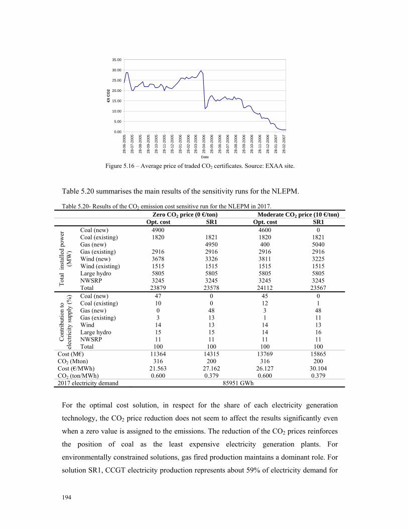
194

0.00

5.00

10.00

15.00

20.00

25.00

30.00

35.00

28-0

6-20

05

28-0

7-20

05

28-0

8-20

05

28-0

9-20

05

28-1

0-20

05

28-1

1-20

05

28-1

2-20

05

28-0

1-20

06

28-0

2-20

06

28-0

3-20

06

28-0

4-20

06

28-0

5-20

06

28-0

6-20

06

28-0

7-20

06

28-0

8-20

06

28-0

9-20

06

28-1

0-20

06

28-1

1-20

06

28-1

2-20

06

28-0

1-20

07

28-0

2-20

07

Date

€/t C

O2

Figure 5.16 – Average price of traded CO2 certificates. Source: EXAA site.

Table 5.20 summarises the main results of the sensitivity runs for the NLEPM. Table 5.20- Results of the CO2 emission cost sensitive run for the NLEPM in 2017.

Zero CO2 price (0 €/ton) Moderate CO2 price (10 €/ton) Opt. cost SR1 Opt. cost SR1

Tota

l in

stal

led

pow

er

(MW

)

Coal (new) 4900 4600 0 Coal (existing) 1820 1821 1820 1821 Gas (new) 4950 400 5040 Gas (existing) 2916 2916 2916 2916 Wind (new) 3678 3326 3811 3225 Wind (existing) 1515 1515 1515 1515 Large hydro 5805 5805 5805 5805 NWSRP 3245 3245 3245 3245 Total 23879 23578 24112 23567

Con

tribu

tion

to

elec

trici

ty su

pply

(%) Coal (new) 47 0 45 0

Coal (existing) 10 0 12 1 Gas (new) 0 48 3 48 Gas (existing) 3 13 1 11 Wind 14 13 14 13 Large hydro 15 15 14 16 NWSRP 11 11 11 11 Total 100 100 100 100

Cost (M€) 11364 14315 13769 15865 CO2 (Mton) 316 200 316 200 Cost (€/MWh) 21.563 27.162 26.127 30.104 CO2 (ton/MWh) 0.600 0.379 0.600 0.379 2017 electricity demand 85951 GWh

For the optimal cost solution, in respect for the share of each electricity generation

technology, the CO2 price reduction does not seem to affect the results significantly even

when a zero value is assigned to the emissions. The reduction of the CO2 prices reinforces

the position of coal as the least expensive electricity generation plants. For

environmentally constrained solutions, gas fired production maintains a dominant role. For

solution SR1, CCGT electricity production represents about 59% of electricity demand for

195

the moderate CO2 price scenario and 61% of electricity demand for the zero CO2 price

scenario.

The reduction of CO2 price will favour CCGT in particular. The average generation costs

of coal power plants would also be reduced for these scenarios, but it seems that the

combination of CCGT with wind power becomes economically more interesting. This

way, although wind power affects CCGT performance, the reduction of the CO2 prices

brings economic advantages to both existing and new CCGT allowing to increase their

electricity production even in the presence of large wind power scenarios.

In general, the reduction of the CO2 price would lead to a reduction of the average

electricity cost. For the Kyoto reference scenario the electricity cost would decline by 3.5

€/MWh for the moderate CO2 price sensitivity simulation and by 6.4 €/MWh for the zero

CO2 price sensitivity simulation.

V.7. Discussion of the results

The development of the NLEPM implied the assessment of the impacts that large wind

power scenarios may have on the Portuguese thermal power system efficiency. The

quantification of these impacts was based mainly on the results of the simulation of the

Portuguese system under different wind power scenarios in 2016 and on the empirical data

characterising the operating conditions of a CCGT power plant.

From the obtained exploration planning, it was possible to conclude that the increase of the

installed wind power would mainly affect CCGT operation. With the exception of the high

growth scenario, where a reduction on the number of operating hours for older coal groups

could be expected, coal power production would remain stable with these plants operating

near full load. The SCGT are minimally affected, because they work mainly as operational

reserve and their load level remains very low for every wind power scenario.

For the CCGT, increasing wind power scenarios affects both the number of operating

hours and the average load level of these thermal power plants. This leads to a growing

inefficiency of these plants, consequently increasing specific gas consumption and specific

CO2 emission factors, and may put in question the value of using wind power to reduce

196

operating costs and to control emissions. However, the results indicate that in spite of this

efficiency loss, both the CO2 abatement and value of wind power still increase with the

increasing wind power in the Portuguese system.

These results are explained partially by the expected particular configuration of the

Portuguese electricity system in 2016, characterised by a large share of hydro power, no

nuclear power plants and the possibility of exchanges with Spain. The incremental wind

power replaces mainly CCGT power and only for high growth wind scenarios there would

be an important effect on the coal power production. However, adding wind power to the

system will increase exports and, as so, the expected reduction of the thermal power

production for large wind scenarios may be offset by the possibility of transmission. The

analysis assumes a fixed non wind capacity in the system, meaning that increasing wind

power will increase the total installed power. Additionally, the evolution of installed wind

power in Spain is not modelled and present market conditions are assumed. This results in

increased capacity of production in Portugal and may explain the large increase in net

exports. This way, the possibility of exchanges smoothes out the variations and the

efficiency of CCGT might not be as affected as it would be in the no transmission case.

Studies for other countries, like Denmark, Ireland and Germany indicate larger CO2

abatement potential, but lower values for the value of wind. However, most of these

studies assume that large amounts of wind added to the system will mainly replace coal

and to a lesser extent gas. Holttinen and Tuhaken (2004) highlighted this issue, underlining

that if gas becomes very expensive, the operating cost of gas plants will rise which will

result in wind power replacing gas instead of coal, as observed in the Portuguese case. This

results in lower environmental gains but is more cost effective. It is also important to point

out that the Portuguese analysis, already takes into account the CO2 emissions cost.

The importance of the hydro power sector in Portugal, might lead to the assumption that

the impact of wind power on thermal system costs would not be significant. However,

from the results it seems clear that although hydropower plays an important role in the

management of the possible wind power fluctuations in Portugal, it will not avoid

important consequences on the thermal power plants performance. In fact, about half of the

total Portuguese hydro power capacity is of run of river type with little or no storage

capacity, presenting this way a low ability to backup fluctuations of the electricity supply

197

or demand.

The run was made for one year, with weekly time steps subdivided in four “hourly steps”

and assuming a weekly average load factor of the wind power plants. This allows to obtain

the average output of each power plant for each one these “hourly steps”, but the effect of

wind power fluctuations during a day is lost. It was however possible to estimate the effect

of seasonal changes on both the wind and hydro sectors. Holttinen and Tuhkanen (2004)

used also weekly time steps for the analysis of the running/dispatch of the Nordic

electricity system for a fixed year. However, Rosen et al. (2007), deal already with the

intradaily problem by presenting a newly developed tool that allows long range planning

based on a hourly load curve and on hourly mean values for the cumulative wind power

feed-in. For the Portuguese case, the daily fluctuations of the wind power may be mainly

compensated by SCGT and hydro power. As so, it is assumed that the power output of the

CCGT and coal power plants will remain close to the average “hourly steps” values

obtained.

According to the 2016 planning, about 21%83 of wind power penetration may be achieved

in Portugal but with some losses of efficiency of the global system. The estimated value of

wind is about 36.5 €/MWh and the CO2 abatement of wind may reach values close to 0.276

tonCO2/MWh. The average variable cost of the system for the high wind growth scenario

is about 27% lower than for the low wind growth scenario. As for the CO2 average

emissions, a 15% reduction may be expected for the high growth wind scenario over the

low growth wind scenario.

The values presented so far result from a fixed analysis of the system, obtained from the

exploration planning based on minimisation of the variable cost. From these results, a

function relating large scale wind production and average operating characteristics of the

CCGT system was estimated. This function was generalised for the planning period and

introduced in the model in an attempt to derive optimal generating strategies for a 10 year

period, taking into consideration the interdependency of the power plants operation and

leading to the NLEPM.

The results of the NLEPM are not directly comparable with the ones reported by the 2016 83 Corresponding to high wind growth scenario (W4) and assuming an average load factor of 26%.

198

exploration planning. Firstly, the 10 year NLEPM aims to optimise the total cost of the

system including the variable and capital costs. While the 2016 analysis assumes certain

scenarios and optimises the operating schedule of the plants in the system (short-run

planning), the NLEPM aims to define the best scenarios describing the mix of the system

and the optimal scheduling (long-term planning). Another important aspect is that the

NLEPM doe not take into consideration the possibility of imports or exports for the

optimisation process and aims to find optimal electricity plans to meet internal demand.

The NLEPM and the EPM, generate rather consistent results. However, there are some

important differences in particular in what concerns the role of wind power in the system.

In the linear model, wind power presents a clear competitive advantage over CCGT,

contributing to both lower costs and emission reductions. As for the NLEPM, increasing

wind shares in the system affect the performance of CCGT plants. For scenarios with high

shares of gas fired units, wind power investments are kept at lower levels although always

ensuring the minimal RES requirements. The combination of CCGT and strong wind

power investments will only be optimal for highly environmentally constrained scenarios.

These results are mainly due to the underlining assumption that coal power performance

would remain largely unaffected by increasing wind shares.

Using the NLEPM also results in higher cost values. For example, the cost of NLS4

(Kyoto reference solution) is about 1.1% higher than S4, assuming similar CO2 levels and

this difference increases for solutions with higher shares of electricity generation from gas

fired units. It also becomes clear that high environmental constraints do not necessarily

lead to high wind power solutions. In fact the results presented in Table 5.16 indicate that

for the Kyoto reference solution, high wind power scenarios could increase total cost by

about 4% while maintaining the same CO2 values. This average cost increase represents a

little less than 1% of the present electricity price paid by the average domestic consumer84

and contributes to a reduction of about 7% on primary energy imports for electricity

production. This exercise suggests that it is possible to increase wind power shares beyond

the optimal costs, with some negative consequences on cost but with important gains in

what concerns external energy dependency and security of supply.

The NLEPM demonstrates that computing the emissions reduction and the operating cost 84 January 2006 values: 14 cent/kWh.

199

increase from wind power using a linear model represents a simplification of the reality.

Onshore wind power remains fundamental to meet the renewable and Kyoto goals, but the

economic advantage of wind over the CCGT detected in EPM is now partly offset.

However, the sensitivity analysis demonstrated that natural gas price increase is

particularly relevant for the decision process and if the European Commission (2006a)

projections become effective, the combination of coal with large wind power scenarios

may become the economically more interesting option even for environmentally

constrained scenarios.

In fact, the sensitivity analysis indicates that the results strongly depend on highly volatile

elements, being particularly sensitive to natural gas price forecasts. The cost of the CCGT

plants depends mainly on their operational costs while for coal power plants the investment

cost is much more relevant than the operational costs. This makes CCGT much more

sensitive to variations on the variable costs (fuel and CO2) and coal power plants much

more sensitive to variations on the discount rate. The effect of these sensitivity simulations

on installed wind power, although visible, is in large extent levelled out by the minimal

RES requirements.

V.8 Conclusions

This study addressed the electricity planning in Portugal using two different models that

differed mainly on the assessment of the impact of wind power on the thermal power

system operation. The models aimed to establish an investment and generation plan for the

electricity system, minimising costs and CO2 emissions during the next 10 years. The

formulation of the models involved extensive data collection from official reports and

information published by the system manager. Some of this information is even considered

confidential and special care had to be taken for its inclusion in the models. It was also

necessary to proceed with the translation of legal and system constraints into mathematical

relationships, in order to adapt the model to the Portuguese conditions. For the NLEPM

additional data was obtained with the REN collaboration on the process.

According to the results, the increasing penetration of wind power in the system will have

significant effects on the CCGT operation and on the theoretically expected cost reduction

and environmental gains. However, opposite to other European studies, the results indicate

200

that the value of wind power and its CO2 abatement potential still present an increasing

trend, partially due to the possibility of exports and to the particular configuration of the

Portuguese electricity system.

As wind power capacity increases, the extra cost of part load operation of CCGT leads to

an increase of their global operating costs. Due to this, the model penalises the

combination of wind and CCGT, favouring the coal-wind power mix in order to minimise

costs. Nervertheless, the model results indicate that under the assumed conditions, the least

expensive way to achieve the Kyoto protocol reference solution (average CO2≤20

Mton/year for the 2008-2017 period) is the strong investment in new CCGT and the

continuous investment in new wind power plants during the planning period.

The results indicate that for low CO2 levels (strongly environmentally constrained model),

the cost minimisation should involve large CCGT investments and not necessarily

maximise wind power in the system. However, solutions with higher wind penetration,

although not optimal from the cost minimisation point of view, might reduce external

energy dependency with the country’s security of supply, compensating for the cost

increase. It seems then, that exclusively relying on the cost aspect for decision making may

be a vision too simplistic for such a complex problem.

Long range energy planning involves forecasting parameters like fuel and CO2 prices,

which is not an easy and straightforward task. The energy market is extremely volatile and

highly sensitive to external problems, politics, government regulation and technological

developments. Although the recent decrease of the CO2 prices might be seen as a sign that

it will be possible to meet the Kyoto objectives without a high financial effort, the futures

market of CO2 still points towards higher prices for the next years. The natural gas prices

increased greatly in 2005 and although some signs of stabilisation are felt in the market,

the prices are still rising. In addition, in March 2007, the European Commission agreed on

the objective to meet 20% of their energy needs with renewables and increase the

emissions cut objective, and set a firm target of cutting 20% of the EU’s greenhouse gas

emissions by 202085.

85 http://ec.europa.eu/energy/energy_policy/index_en.htm

201

As Hobbs (1995) states “no one resource plan will be the best under all possible futures”.

The sensitivity analysis showed that the planning process is very responsive to variations

on the parameters, and the recent developments of the market clearly demonstrate that a 10

year period involves a lot of uncertainty: the relationship between fuel prices may change,

the CO2 prices may contribute to this change or become a major cost source and the legal

environment will certainly suffer modifications. However, it seems obvious that the trend

in the EU is towards increasing the RES share. Wind power has the clear advantage of

having operational costs invulnerable to fuel and emisisons market volatility. In fact, the

only certain element of the planning model is that, regardless of politics and of the market

behaviour, in 10 years wind will still be blowing for free.

Wind power has as a fundamental role on meeting the renewable and Kyoto protocol’s

commitments. For all the scenarios analysed and regardless of the sensitivity simulations

performed, installed wind power must reach at least 4740 MW in 2017 and careful

management of the hydro sector must be ensured. For most of the solutions, total installed

wind power converges to values close to 5000 MW or even higher. Portugal has the

possibility of extensively using the hydro sector for the management of large wind power

levels in the system and, the planning studies of the Portuguese generating system,

concluded that the use of hydro schemes with reversible capacities to ensure the adequate

levels of security of supply is the most appropriate solution. Therefore, it is fundamental to

proceed with the planned hydro schemes in order to avoid possible situations of

operational reserve deficit (Esteves et al., 2003). At the same time, these hydro schemes

represent an important contribution to meet the RES goals established for Portugal

(Ferreira et al., 2007a). Hydro power production can actively contribute to reduce the

effect of wind power on thermal power operation, but as the results demonstrate these

effects are still significant and should not be disregarded in the electricity planning process.

A previous study (Saleiro et al., 2007) analysed the cost of the electricity generation

options, based on private and external costs of generation in Portugal. The study concluded

that the financial cost of wind power is still higher than the CCGT, but when the external

costs are considered the results change and the CCGT reaches cost values close to the wind

power or even higher. However, these techniques used to study the generation alternatives,

even when considering the externalities and avoided cost and emissions, tend to ignore the

interaction between all the elements in the electricity system, which are fundamental for

202

long range planning. The present study intends to go beyond the economic evaluation of

the individual electricity generation options. The presented models allow dealing with a

complex and dynamic model, recognising that planning and operating decisions regarding

one generation option should not be taken individually, because this will strongly affect the

entire system.

The aim of the electricity planning models was to provide a description of the Portuguese

electricity system in a 10 year period, giving particular emphasis to the coal-natural gas-

wind power mix. The models allowed the presentation of a plant scheduling for a large

range of CO2 scenarios, describing the role of thermal and wind power production.

Comparison of the models have shown that wind power will affect CCGT performance and

not taking into account this element will result in overestimation of the economic and

environmental value of wind power.

The difficulties in data collection and in the modelling process, required the assumption of

simplifications in the models. However, the presented models have made some important

contributions and can give a global overview of the future of the electricity system in

Portugal under the assumed constraints, in view of the expected demand and of the fuel

prices. Regardless of all the limitations, the NLEPM may be seen as an exploratory model

that succeeds on demonstrating the need to develop integrated planning tools for medium

to long term electricity planning.

V.8.1 Limitations and research requirements

The present models include only two objectives: cost and CO2 emissions. Future models

may be extended to include other objectives, in particular from the environmental field.

Also, the model may be refined to allow for the integration of other renewable energy

sources or clean coal technologies as additional variables. The possibility of CO2 capture

for thermal power plants must be regarded. According to the model, surpassing the present

Kyoto commitments would imply keeping coal power production at very low levels or

even disinvest completely on it. This would represent an important risk from the security

supply point of view with an almost exclusive reliance on natural gas. Sustainable coal

technologies can overcome the environmental problems of ordinary coal power plants and

must be included in the model as another option for clean electricity production. In fact,

203

the recent EU documents (Commission of the European Communities, 2007a) indicate that

not only renewable energy is a priority but also the introduction of CO2 capture and

storage.

The NLEPM coupled the results of the analysis of the Portuguese electricity system in

2016, with the dynamic planning process for the 10 year period. Ideally the 2016 strategies

should be designed using small periods of analysis, which should capture the instantaneous

effect of wind on the operation of conventional thermal power plants. An important

limitation of this approach is the theoretical assumption that the results obtained from the

2016 exploration planning could be generalised and included in the planning model. This

rough approach treats the CCGT system as a whole and models the operating conditions

according to general behaviour of a set of groups. It assumes that the impact of wind on the

CCGT system would be the same regardless of the system characteristics and that the

performance of coal power plants would remain unaffected regardless of the installed wind

power.

Ideally, the process should be iterative and based on a complementary approach,

combining long term energy expansion plans with the results of short term operation

strategies for each one of these plans. This approach allows for the inclusion of wind

power impacts on the system performance within long term capacity expansion and

electricity production planning, as described in Figure 5.17. For this particular study, the

long range planning could be conducted for a 10 year period divided in monthly intervals.

The short term planning should be conducted for a one year period divided in periods of an

hour length for more effectively capture the wind power variability.

Further development of the Portuguese model would strongly benefit from close

collaboration with the system manager, and further attempts will be made to involve this

entity in the process with particular emphasis on the dispatching rules. In a recent study,

Rosen et al. (2007) recognise the importance of this issue and present new tools for the

integration of wind power effects on power plant scheduling with the optimised evolution

of the future power system structure. This desirable collaboration with the system manager

would also help developing future versions of the models taking into consideration two

other essential aspects: (i) the integration of the Portuguese electricity system in the Iberian

market and consequently the possibility of trading with Spain and (ii) the estimated grid

204

costs for integration of decentralised electricity producers.

Short termplanning model

Long termplanning model

Capacityexpansion plan

Short termoperation scheduling

Impacts on the operation of thermal power plants

Optimal capacity expansion

and electricity production plans












Optimal capacity expansion

and electricity production plans

Figure 5.17- Proposed model coupling long and short range planning.

The resource planners’ task is now much more complex and along with dealing with

several technological options and uncertainty, resource planning must also take into

consideration that the objectives expanded beyond cost and even beyond direct

environmental impacts (Hobbs, 1995). So far, the study considered a multiple objective

energy planning optimisation model where the environmental and economic objectives

were described by mathematical functions. The results were a set of compromise solutions

detailing plans for new thermal and wind plant installations over a ten year planning

horizon for Portugal. However, finding the Pareto optimal solutions is just the first step to

resolve the planning problem. A broader multi-perspective evaluation approach is

fundamental, measuring and assessing the qualitative impacts of the possible power

scenarios and their social acceptability. The subsequent stage of the research was more

oriented towards the agents’ perspective and called for additional information, based

frequently on non technical, qualitative and experience driven factors. The social

dimension of the problem was addressed by a participative process, collecting value

judgments regarding the definition of the most relevant impacts and their importance.

CHAPTER VI

INTEGRATING SOCIAL

CONCERNS INTO

ELECTRICITY PLANNING

This chapter proposes a support framework, combining Delphi and AHP

methodologies, to accommodate social concerns in the electricity planning

process. The process calls for the involvement of a group of experts,

participating in the social evaluation of the electricity generation options. The

results highlight the complexity and subjectivity of the issues in question, but

also suggest that a social impact index may be used as a first indicator of

society’s acceptance of the plans drawn from the mathematical optimisation

models.

207

VI.1 Introduction

Social, technological, economic and environmental issues should be considered

comprehensively in the evaluation of the electricity planning options. The developed

electricity planning model (EPM) and non-linear electricity planning model (NLEPM)

presented in the previous Chapter, include assessment of quantitative factors, but, do not

explicitly consider such factors as noise, visual impact or social acceptance. As highlighted

by Söderholm and Sundqvist (2003), many impacts of the power generation sector involve

moral concerns and economic valuation provides an insufficient basis for social choice.

In this chapter, the Analytic Hierarchy Process (AHP) and the Delphi methodology are

combined to assess the social impact of the different technologies for electricity

production. The results of this research may be integrated with the NLEPM, resulting in a

new methodology for evaluation of the electricity generation solutions from the

environmental, economic and social points of view.

The core elements of the study are the Delphi survey and the AHP analysis. By

subdividing the problem into its constituent parts (Analytic Hierarchy), the problem is

simplified and allows information on each separate issue to be examined. The relative

strength or priority of each objective can be established (Delphi process) and the results

synthesised, to derive a single overall priority for all activities (Hemphill et al., 2002).

The combination of the AHP and Delphi has been used in different fields, with the aim of

quantifying the value judgment obtained in a group decision making process. Some recent

examples include works from Hemphill et al. (2002), on the weighting of the key attributes

of sustainable urban regeneration, and Zhong-Wu et al. (2007) for the appraisal of the eco-

environmental quality of an ecosystem. Banulus and Salmeron (2007) proposed a Scenario

Based Assessment Model integrating both AHP and Delphi methods to support long-term

technology policies. Another recent example is the adoption of the Delphi method and

AHP for developing an evaluation method to select the optimal location of a regional

hospital (Wu et al., 2007). Chen and Liu (2006) presented a new methodology for

evaluation and classification of rock mass quality on tunnel engineering based on

combined AHP and Delphi methods. Likewise, Hon et al. (2005) combined both methods

on a performance evaluation model applied to third party logistics. Liang et al. (2006)

208

presented a power generation expansion model that uses AHP and Delphi methodologies.

In this chapter we deal with the complexity of the social issues surrounding electricity

planning. A methodology is proposed establishing a possible way of allocating weights to

the major social impacts and resulting in a final scoring of the electricity generation

options. The process involved the following steps:

1. The identification of difficult to quantify attributes and options to analyse. This step

corresponds to the definition of the social criteria to select the best electricity

generation options, from the social point of view.

2. The establishment of a hierarchical structure. The top of the hierarchy is the main

goal corresponding to the social index and the lower levels describe the criteria. On

the bottom level we have the discrete alternatives of the problem, corresponding to

the electricity generation options.

3. Selection of a group of experts and establishment of the pairwise comparison of the

elements of the hierarchical structure. The Delphi method is used to collect this

information.

4. Testing the consistency of the data collected from the experts.

5. Aggregation of the scores collected from the experts. From this step results the

relative weights of the elements of each level of the hierarchical structure,

reflecting the group judgment.

6. Combine the relative weights of the elements of each level of the hierarchical

structure, obtaining the final scoring of the electricity generation options against the

overall social objective.

This introduction outlines the process of social evaluation of the electricity planning

options. The following Sections VI.2 and VI.3 provide a description of the AHP and

Delphi methods. Some examples of their application are drawn from the recent literature,

justifying also their suitability for the electricity planning problem. The use of these

209

methods for the social ranking of electricity generation options in Portugal is described

from Section VI.4 onwards. Section VI.4 describes the hierarchical structure formulation

including the options analysed and criteria considered. Section VI.5 details the

implementation of the Delphi study based on a questionnaire sent to a pilot group of

experts. Section VI.6 combines the information obtained from the Delphi process with

AHP in order to derive a social index ranking the electricity generation alternatives.

Section VI.7 discusses the results obtained. The incorporation of the social index in the

overall planning process is presented in Section VI.8, where the results of this social

analysis are integrated with the results of the previous mathematical optimisation

procedure, resulting in a new integrated electricity planning model. Section VI.9 draws the

conclusions of the chapter pointing out the main limitations of the work and indicating

directions for future research.

VI.2 Overview of the AHP method

The AHP addresses and analyses discrete alternative decision problems with multiple

conflicting criteria. This technique allows qualitatively based data to be transformed into

pairwise comparison data. The decision problem is reduced to a series of smaller self-

contained problems. The relative merit of each option is determined from the pairwise

analysis of their relative performance ratings. The result of the overall process is a ranking

of all the alternatives on an interval scale (Rogers, 2001).

The AHP model uses a hierarchical structure to represent the problem typically

representing the overall objective or goal of the decision-making process at the top level,

criterion or attribute elements affecting the decision at the intermediate level, and the

decision options at the lower level (Nigim et al., 2004). The user chooses weights by

comparing attributes two at a time, assessing the ratios for their importance. These ratios

are used not only to compute the weights of individual attributes, but also to measure the

consistency of the user’s assessments (Hobbs and Meier, 2003).

Zhong-Wu et al. (2007), considered AHP to be a simple systematic engineering method to

quantitatively analyse non-quantitative criteria. The method incorporates the researcher’s

subjective judgment aided, if needs be, by expert opinion during the analysis, and by

expressing the complex system in a hierarchical structure. Thus, AHP assists the decision-

210

making process to be systemic, numerical and computable. Also, it assesses the

consistency of the judgment and incorporates the evaluations of all decision makers into a

final decision, without having to elicit their utility functions on criteria (Wu et al., 2007).

According to Liang et al. (2006) “AHP is a systematic method that captures a human

being’s mind process in mathematically hierarchical levels”.

AHP is a popular method in problem evaluation (see for example Hobbs and Meier, 2003,

Limmeechokchai and Chawana, 2007 or Liang et al., 2006) and has been extensively

applied in dealing with complex energy and environmental problems. Pohekar and

Ramachandran (2004) presented a literature review on multi-criteria decision making on

sustainable energy planning, and observed that AHP is the most popular technique.

Hobbs and Meier (2003), give some examples of AHP usage in the evaluation of the

environmental impacts of power planning options, in the selection of greenhouse

mitigation options, in the evaluation of electricity supply plans and in the development of

national energy policy. Lee et al. (2007) used an AHP approach to determine priorities in

technology development for energy efficiency and greenhouse gas control plans in Korea.

Liang et al. (2006) included AHP in their model for evaluating power generation projects.

Other examples in energy related sectors include: the prioritisation of barriers to energy

efficiency in small industry clusters (Nagesha and Balandra, 2006), the identification and

prioritisation of barriers to particular sustainable energy development strategies

(Limmeechokchai and Chawana, 2007), the prioritisation of local renewable energy

projects (Nigim et al., 2004) or the prioritisation of energy conservation policy instruments

(Kablan, 2004), among many others. An extensive list of examples may be found in

Greening and Bernow (2004) or Pohekar and Ramachandran (2004).

VI.2.1 The AHP process

The analytical hierarchy process was developed by Saaty (1980) and is based on the

formulation of the decision problem in a hierarchical structure, like the one presented in

Figure 6.1. The process involves the following main steps:

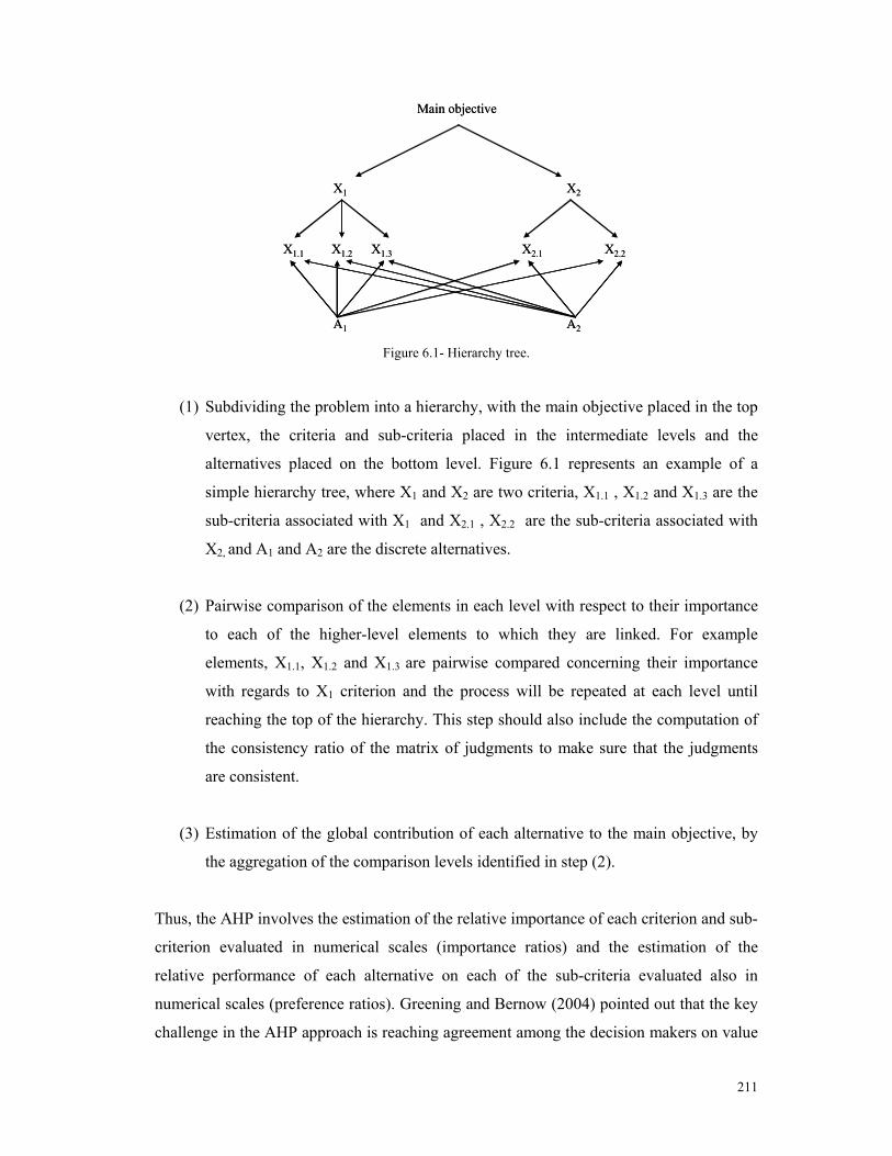
211

Main objective

X1 X2

X1.1 X1.2 X1.3 X2.1 X2.2

A1 A2

Main objective

X1 X2

X1.1 X1.2 X1.3 X2.1 X2.2

A1 A2 Figure 6.1- Hierarchy tree.

(1) Subdividing the problem into a hierarchy, with the main objective placed in the top

vertex, the criteria and sub-criteria placed in the intermediate levels and the

alternatives placed on the bottom level. Figure 6.1 represents an example of a

simple hierarchy tree, where X1 and X2 are two criteria, X1.1 , X1.2 and X1.3 are the

sub-criteria associated with X1 and X2.1 , X2.2 are the sub-criteria associated with

X2, and A1 and A2 are the discrete alternatives.

(2) Pairwise comparison of the elements in each level with respect to their importance

to each of the higher-level elements to which they are linked. For example

elements, X1.1, X1.2 and X1.3 are pairwise compared concerning their importance

with regards to X1 criterion and the process will be repeated at each level until

reaching the top of the hierarchy. This step should also include the computation of

the consistency ratio of the matrix of judgments to make sure that the judgments

are consistent.

(3) Estimation of the global contribution of each alternative to the main objective, by

the aggregation of the comparison levels identified in step (2).

Thus, the AHP involves the estimation of the relative importance of each criterion and sub-

criterion evaluated in numerical scales (importance ratios) and the estimation of the

relative performance of each alternative on each of the sub-criteria evaluated also in

numerical scales (preference ratios). Greening and Bernow (2004) pointed out that the key

challenge in the AHP approach is reaching agreement among the decision makers on value

212

judgements of the importance of the elements.

Hon et al. (2005) describes the major steps of the AHP methodology: build pairwise

comparison matrix, eigenvalue and eigenvector calculation, review of the consistency of

the matrix and normalize criteria weight. These authors consider that the AHP method

obtains a weighting of the criteria through the paired comparison between every criteria

pair within each level, which is more credible and more objective than overall subjective

judgments set directly by decision making managers.

The values used for the pairwise comparison are usually based on Saaty scale of

preferences, presented in Table 6.1.

Table 6.1- Saaty’s scale of preferences in the pairwise comparison process (Saaty, 1980)

Score Pairwise evaluation 9 A absolutely more important than B 7 A is very strongly more important than B 5 A is strongly more important than B 3 A is moderately more important than B 1 A is equally important to B

1/9, 1/7, 1/5, 1/3, 1 Reciprocal values

For this particular research, the aim was to address the negative social impact of each

generating technology86. For the comparison a scale based on Saaty (1980) proposal was

used, detailed in Table 6.2.

Table 6.2- Scale preferences used in the pairwise comparison process.

Range Category

Superior

Absolutely superior Very strongly superior

Strongly superior Moderately superior

Equal Equal

Inferior

Absolutely inferior Very strongly inferior

Strongly inferior Moderately inferior

Table 6.3 represents a pairwise comparison matrix, with the elements representing the

quantified judgment on a pair of solutions. The matrix used in the example was drawn

from the results obtained for the pairwise comparison of the three possible generation

86 A particular technology assigned a higher score is considered “worst” from the social point of view than a technology assigned with lower score.

213

technologies against noise impact, provided by one of the experts.

Table 6.3 - Pairwise comparison of the alternatives with respect to the noise impact.

Coal Gas Wind Coal 1 1 1/3 Gas 1 1 1/5

Wind 3 5 1

When an alternative is compared with itself each alternative has equal weight. This makes

the diagonal elements of the matrix always equal to 1. The entries below the diagonal are

the reciprocal of those entries above the diagonal. This implies that only the judgements in

the upper triangle of the matrix need be solicited (Kablan, 2004). The matrix above (Table

6.3) shows for example that for this expert, the noise impact of coal solution is equal to the

noise impact of gas solution. The noise impact of the wind solution is strongly superior to

the noise impact of the gas solution and moderately superior to the coal solution87.

For the computation of the weights AHP follows the eigenvector analysis, as described in

Kablan (2004). Assuming that the decision maker is capable of making pairwise

comparasions between different alternatives (A1, A2,… An), these may be represented as in

the following matrix:

⎥⎥⎥⎥

⎦

⎤

⎢⎢⎢⎢

⎣

⎡

=

ann...an2an1............

a2n...a22a21a1n...a12a11

An..

A2A1

A

An .... A2 A1

The values assigned to aij are usually in accordance with Saaty scale presented in Table

6.1. A is then a consistent matrix of judgment and Saaty’s (1980) method computes K

(vector of weights) as the principal right eigenvector of the matrix A:

87 Wind technology is then considered “strongly worst to society” than gas technology, from the noise impact point of view. The same way, wind technology is considered “moderately worst to society” than coal technology, from the noise impact point of view.

214

⎥⎥⎥⎥

⎦

⎤

⎢⎢⎢⎢

⎣

⎡

=

⎥⎥⎥⎥

⎦

⎤

⎢⎢⎢⎢

⎣

⎡

⎥⎥⎥⎥

⎦

⎤

⎢⎢⎢⎢

⎣

⎡

Wn...

W2W1

λ

Wn...

W2W1

ann...an2an1............

a2n...a22a21a1n...a12a11

or AK=λK (6.1)

(A-λmax Z)K=0 (6.2)

Where λmax is the largest possible value of an eigenvalue (λ) of matrix A and Z is the

identity matrix and K is the eigenvector.

If the pairwise matrix is perfectly consistent then λ will be equal to the number of

alternatives under consideration (n). The consistency index (CI) and the random

consistency index (CR) may be computed by (Kablan, 2004):

1nnλCI max

−−

= (6.3)

RICICR = (6.4)

The consistency ratio is a measure of how a given matrix compares to a purely random

matrix in terms of their consistency indices. The value of the random index (RI) may be

obtained from published tables for each size of the matrix, n (see for example Kablan,

2004 or Lee et al., 2007). In practice if CR≤0.10, the consistency of this matrix is

acceptable (Zhong-Wu et al., 2006; Hon et al., 2005, Kablan, 2004).

For the computation of the weights and the consistency ranking, the software package

Super Decisions was used. This software was developed by the Creative Decisions

Foundation and is freely available in the internet (http://www.superdecisions.com). The

input to the software is the hierarchical structure of the problem and the pairwise

comparison matrices of the attributes. The output includes the weighting matrices, the

evaluation of the consistency of the judgments and the final ranking of the options.

215

For the particular example of matrix A presented in Table 6.3, Saaty’s (1980) method may

be applied to derive the vector of weights detailed in Table 6.4 along with the consistency

ratio:

⎥⎥⎥

⎦

⎤

⎢⎢⎢

⎣

⎡=

⎥⎥⎥

⎦

⎤

⎢⎢⎢

⎣

⎡

⎥⎥⎥

⎦

⎤

⎢⎢⎢

⎣

⎡

wind

gas

coal

wind

gas

coal

WWW

WWW

1535/1113/111

λ (6.5)

Table.6.4 – Vector of weights of the alternatives with respect to the noise impact.

Noise impact Gas 0.156 Coal 0.185 Wind 0.659

CR 0.0280 As expected, the weights sum to 1.0. For this particular expert as far as noise is concerned,

gas is the most desirable solution, followed by coal generation plants with wind generation

being the least desirable. Since the consistency ratio is below 10% then the judgements are

considered consistent, although the consistency is not perfect. In perfect consistency

conditions, if the noise impact of the coal solution is equal to the noise impact of the gas

solution, the score between the coal and gas solutions respectively with the wind solution

should be the same. If that were the case, the CR would equal zero.

VI.2.2 Suitability of the AHP approach.

The AHP is especially suitable for complex systems where multiple options and multiple

criteria are to be taken into consideration. The computation of a social index for a complex

problem like the electricity generation options involves individual judgments and it can be

described and analysed using a hierarchical structure. The AHP was selected because of its

simplicity and ability to deal with qualitative/subjective data. The qualitative scale used

simplifies the judgement but at the same time allows for the mathematical treatment of the

results. The final outcome is the global ranking of the options.

AHP is recognized as a robust and flexible tool for dealing with complex decision making

problems (Liang et al., 2006) and its use has been largely explored in the literature with

many examples in the energy decision making field. This method is well suited for group

216

decision making (Lai et al., 2002) and its integration with the Delphi method is also well

documented (see Section VI.1). Using the hierarchical structure, the experts compare the

electricity generation options against different criteria. It is possible to recognize conflicts

among experts for each element of the hierarchy, how it affects the final ranking and also

the consistency of the judgments.

VI.3 Overview of the Delphi method

The main objective of the Delphi technique is to describe a variety of alternatives and to

provide a constructive forum in which consensus may occur (Rayens and Hahn, 2000). The

three basic conditions of the process are: anonymity of the respondents, statistical

treatment of the responses and controlled feedback in subsequent rounds.

The anonymity of the answers gives group members the freedom to express their opinion,

avoiding possible negative influences due to previous assumed positions, status of the

participating experts and reluctance on assuming positions different from the general

opinion or from a dominant group.

The statistical treatment of the responses allows the assembly of collective information.

This phase feature ensures that all the opinions form part of the final answer and that these

opinions may be communicated to the panel without revealing individual judgments.

Delphi study presents the statistical result that includes the opinion of the entire group,

presenting both the centre of the group opinion and the degree of spread about the centre

(Institute for Prospective Technologic Studies, 1996).

The experts must be consulted at least twice so that they may reconsider their answer,

aided by the information received from other experts. This feedback is controlled, so that

all irrelevant information is eliminated (Landeta, 2006) and the panel individuals have

access to the responses of the whole group as well as their own response for

reconsideration. Often, feedback is presented as a simple statistical summary of the group

response, usually comprising a mean or median value. Occasionally, additional

information may also be provided, such as arguments from the individuals (Rowe and

Wright, 1999a).

217

The interaction among group members taking place in a controlled and anonymous manner

distinguishes Delphi from the conventional face-to-face interaction. At the end of the

procedure the group judgement is taken as a statistical measure of the participants’

estimates. This final judgement may be seen as an equal weighting of the opinions of the

participants (Rowe and Wright, 1999a).

The basic sequence of the Delphi method may be resumed as an interactive questionnaire

that is passed around several times in a group of experts, keeping the anonymity of the

individual responses. In the first round the experts receive a written questionnaire or are

asked to participate in a interview. This first questionnaire usually describes in detail the

issue in question and contains information that may help the respondents to answer the

questions and ensures a reasonable homogeneity of the knowledge and language used

(Wright and Giovinazzo, 2000).

The initial measurement of opinions is followed by the data analysis. Based on the group

responses to the first questionnaire, a new questionnaire is developed where the statistical

results of the first round and information on the beliefs of other participants are presented.

This process allows participants to reconsider their opinions in light of the views of the

other elements of the panel and may be repeated until consensus is reached or the

polarisation is well established (Rayens and Hahn, 2000). When participants reach

consensus in a question, it is omitted from succeeding iterations (Alberts, 2007).

As Wright and Giovinazzo (2000) stated the Delphi is not a statistical representative study

but a process of collecting opinions from a group of experts, who from their knowledge

and exchange of information may achieve comprehensive opinions on the proposed

questions. This issue is also pointed out by Okoli and Pawlowski (2004), who underlined

that the questions that a Delphi study investigates are those of high uncertainty and

speculation. Thus a general population or sample might not be sufficiently knowledgeable

to answer the questions accurately.

The Delphi method is frequently used to forecast tendencies and future events. Matias

(2002) used a Delphi approach on the design of future energy scenarios in Portugal. Blind

et al. (2001) used a two round Delphi expert survey focusing on the estimation of the

future development of science and technology in Germany. The Institute for Prospective

218

Technological Studies refers and uses the Delphi method as a forecasting tool (see for

example Institute for Prospective Technological Studies, 1996, 2000 and 2002). Iniyan and

Jagadeesan (1997) used a Delphi study to determine the social acceptance and percentage

use of renewable energy sources in the future. A Delphi study was also conducted for the

assessment of changes in the international business environment over the next decade and

the evaluation of the impact of these changes on policy and on corporate practices

(Czinkota and Ronkainen, 2005).

However, as stated by Rayens and Hahn (2000), Delphi technique is also an appropriate

tool for the definition of policies and for decision making, enabling the description of

agreement on specific policy options (policy Delphi). OECD (2006) suggests some

examples of tools that could be used in the context of strategic environmental assessment

approaches. This report points out that expert judgement of direct and indirect impacts is

relatively quick and cheap and that it can be used in applications like collecting data,

developing alternatives from the strategic policy level to the detailed site level, analysing

and ranking them, predicting impacts, and suggesting mitigation measures. Also the Guide

for evaluation of socio-economic development in Europe (Tavistock Institute, 2003)

includes Delphi panel as a key method for interventions in the energy sector.

Rayens and Hahn (2000) report the use of policy Delphi method in building consensus on

tobacco policy issues in Kentucky. Also Jillson (2002) describes a previous study

conducted in the USA, using Delphi procedures in the exploration of the national drug-

abuse policy that has raised considerable interest in the utilisation of the technique not only

in the drug-abuse field, but in other social policy areas as well. Wright (2006) describes a

Delphi method used on the generation of an implementation plan for university

sustainability policies. Loe and Wojtanowski (2001) used a two-round policy Delphi

survey for assessing the associated benefits and costs of the Canada's Flood Damage

Reduction Program. Okoli and Pawlowski (2004) presented some examples of publications

using the Delphi method as a tool in information systems research to identify and prioritise

issues for managerial decision-making and to forecast the business future. The Lawrence

Technological University conducted Delphi inquiries on how to address wind turbine noise

and potential wildlife impacts (Alberts, 2007). The participation on the study was opened

to public, including stakeholders, public policy makers and concerned citizens. However,

the results showed that participants with insufficient experience were unable to participate

219

effectively in the decision making process, demonstrating that it can be more productive to

seek input from technical experts than to seek consensus from all stakeholders.

VI.3.1 The Delphi process

Figure 6.2 summarises a general Delphi process.

Choice of the subject

Choice of the topics

Selection of the experts

Writing of the questionnaire

1st round

Statistical analysis of the results

Re-writing of the questionnaire

New round


Consensus or stability No consensus or stability

Conclusions

Choice of the subject

Choice of the topics

Selection of the experts

Writing of the questionnaire

1st round


Re-writing of the questionnaire

New round


Consensus or stability No consensus or stability

Conclusions Figure 6.2- General Delphi process.

The first phase is characterised by the description of the subject to study and of the

objectives of the research. Based on this, the specific topics to be addressed are defined

and the experts are chosen. The selection of the experts is a crucial phase because the

quality of the results depends heavily on the knowledge and commitment of the

participants. According to Scapolo and Miles (2006), the minimum size of a panel of

experts to involve in a Delphi exercise should be no less than 8 to 10. Rayens and Hahn

(2000) also indicate that in a typical policy Delphi the number of participants varies

between 10 and 30.

The research team contacts the experts explaining them the basis of the Delphi technique,

220

the objective of the research and their role in the process. Usually the questionnaires are

sent by post or email although collecting the responses with in-person interviews may also

be possible. The responses of this first round are collected and the research team proceed to

the statistical analysis. After analysing the results a new questionnaire is elaborated. The

participant’s response on the first enquire determine modifications through each iteration

(Alberts, 2007). The new questionnaire presents the results of the first round; it frequently

includes comments received during the first round, new questions may be added and some

other questions may be eliminated.

The rounds continue until a satisfactory level of convergence is achieved. According to

Wright and Giovinazzo (2000), at minimum the study should have two rounds and usually

is does not overcome three rounds. Alberts (2007) refers that the ending of the process may

depend not only on reaching consensus but also on project funding. Scapolo and Miles

(2006) restricted the number of rounds to two, in order to limit as much as possible the

weariness of the participants and their possible pressure for conformity. Also Rayens and

Hahn (2000) limited the policy Delphi process to two stages due to potential for participant

attrition and budget constraints.

The approach to measuring consensus varies from study to study. Rayens and Hahn (2000)

present some examples of measures used in past studies such as:

The frequency distributions. The criterion of at least 51% responding to a certain

category may be used to determine consensus, or at least 67% in a yes-no study, as

presented in the following example for two possible questions. Example 1

Question A Question B Response % of responses Response % of responses Strongly agree 20% Agree 80% Agree 58% Disagree 20% Neither agree or disagree 4% Disagree 15% Strongly disagree 3% Consensus Achieved Consensus Achieved

In studies where the participants are asked to rank or weight ideas, the mean values

and standard deviation may be computed in each round. A reduction of the

standard deviation indicates higher degree of consensus achieved after successive

221

rounds.

Another popular approach is the interquartile range (IQR), measuring the absolute

value of difference between the 1st and 3rd quartile, with smaller values indicating

higher degree of consensus. The interpretation of this measure varies between

authors and of course depends on the number of response choices. Rayens and

Hahn (2000) identified an IQR of 0.00 as an indicator of consensus. These authors

assumed also that consensus was achieved if the IQR was equal to 1.00 and the

percentage of generally positive or negative responses were higher than 60%. By

using this strategy the authors could deal with a larger number of response choices

or categories. An example is presented next: Example 2

Question A Question B Response % of responses Response % of responses Strongly agree 49% Strongly agree 21% Agree 39% Agree 61% Disagree 11% Disagree 16% Strongly disagree 1% Strongly disagree 2% IQR 1.00 IQR 0.00 Consensus Achieved Consensus Achieved

In a different work, Loe and Wojtanowski (2001) assumed:

• high consensus if at least 70% of the participants chose one particular

category or at least 80% of the participants chose two related categories,

• low consensus if at least 50% of the participants chose one category and

60% of the participants chose two related categories and

• no consensus for less than 60% rating in two related categories.

Dorussen et al. (2005) also detail some measures of agreement in experts interviews.

However, these measures only apply if the number of possible answer categories is fairly

small. In their study the experts were asked to choose between two and five possible

categories. Rowe and Wright (1999b) present an analysis of some measures extensively

used in the literature to determine consensus achievement, including the variance reduction

and the post-group consensus.

Most Delphi studies are consensus oriented and it is assumed that this consensus is

222

achieved when a certain percentage of answers fall within a certain category or a certain

value of IQR is achieved. Scheibe et al. (2002) indicate as a possible IQR cuttoff value two

units in a ten unit scale. These authors also present an additional measure which takes into

consideration the stability of the respondents’ vote distribution curve over successive

rounds of the Delphi. This way the method measures the amount of change in the group

opinion rather than the amount of change in each individual’s vote between rounds. The

authors propose the 15% change level as the ‘state of equilibrium’.

Combining the stability and consensus measures allows the identification of well defined

disagreement aspects as well as aspects of agreement within the participating group. As

Landeta (2006) pointed out, the restriction of the obligatory search for consensus may be

eliminated and the Delphi technique may be described as a social research technique which

aim is to obtain a reliable group opinion using a group of experts. Linestone and Turoff

(2002) also characterise the Delphi technique as “a method for structuring a group

communication process (…) allowing a group of individuals, as a whole, to deal with a

complex problem”. Landeta (2006) draws attention to the contrast between the apparent

simplicity of the technique and the work and difficulty involved in its execution. These

difficulties include ensuring the initial collaboration of the experts and particularly their

commitment to the process in different rounds.

A more detailed description of the Delphi method may be found in Linstone and Turoff

(2002), along with its historical development and examples of application. Also Landeta

(2006) reviews the literature in this area and presents some examples of application. Rowe

and Wright (1999b) compile published studies involving evaluation of the Delphi

technique.

VI.3.2 Suitability of the Delphi approach

The Delphi method was selected for information collection in this particular research for

the following reasons:

The questions addressed are complex and highly subjective. Using a panel of

experts with previous knowledge and interest in the matter in question seems to be

the most productive way to collect opinions.

223

The anonymity of the responses eliminates the influence of dominant position, the

conflict between participants or the reluctance on changing previous assumed

positions. But as the participants are only anonymous to each other and never to the

researcher, it facilitates the follow-up process. In fact, this allowed phone contact

with the non respondents increasing the response rate.

The structured questionnaire ensures a proper collection of information, in a way

that may be easily incorporated in the AHP analysis.

It does not require the experts to meet physically, which allows them to answer the

questioner in their own workplace and when they find appropriate.

The Delphi process is a time consuming task, due to the iterative process. However

for this particular research, the panel size was kept modest and the questionnaires

were sent by email, which allowed the process completion in about three months.

The literature indicates that the non-response is typically low in Delphi surveys

(Okoli and Pawlowski, 2004).

VI.4 Hierarchical structure formulation

As the analysis is to be carried out using the AHP a hierarchical structure describing the

problem must be designed. For this elements of the different levels of the hierarchy and

their relationships must be identified.

VI.4.1 Options or alternatives.

The process started with the identification of the options to be analysed. Based on the

optimisation models presented in chapter V, three electricity generation options were

included: coal, gas and wind. However, we do not expect the development of the

Portuguese electricity system to be based only on one of these generation options, and the

most probable scenario will include the combination of the three technologies.

For comparison of the alternatives the evaluation was based on the marginal increase of the

224

demand and the corresponding increase of each one of the generation options. For a

marginal increase of 1000 MW of the electricity demand88, the corresponding increase of

the generation options was defined. From the AHP analysis, a social index representing the

social evaluation of these options may then be obtained. The overall social evaluation of

the possible combined scenarios will be drawn from these individual indices.

VI.4.2 Criteria

The next step was the identification of the criteria to be included in the evaluation process.

Choosing these criteria is essential for the proper establishment of the social index. The

criteria should be able to represent the main social (or non quantifiable) features of the

system. From existing literature addressing the social impact of the electricity generation

technologies and from discussions with experts in the energy field, the criteria considered

relevant were defined.

The public perception of wind power is addressed by several authors for a number of

countries or regions. Some examples of research studies on this field include Ek (2005),

Wolsink (2000), Manwell et al. (2005) or Bergmann et al. (2006) among many others89.

Most of the studies identified as positive aspects the renewable characteristic of wind

power and the avoided emissions. On the other hand, in most of the publications there is a

predominant emphasis on the negative visual impact on the landscape. Other identified

negative impacts include: the impacts on wildlife, the noise pollution, the unreliability of

wind energy supply and the possible financial cost, with particular emphasis on the first

two aspects.

Studies addressing the coal and gas power plants impacts deal mainly with the cost and

environmental emissions (see Rafaj and Kypreos, 2007 or Soderholm and Sundqvist,

2003). The environmental impact usually focuses on the damages caused to health and on

the impact on climate change. In the ExternE project, the external effects from coal and

natural gas power plants were mainly associated with their pollutant emissions and their

impact on public and occupational health, agriculture and forests. The noise problem was

also pointed out, including operational and traffic impact.

88 This value corresponds to about 17% of the average load in 2006. 89 This issue is longer debated in Section IV.3.3 of this thesis.

225

VI.4.2.1 Semi-structured interviews with experts

Following the literature analysis, semi-structured interviews were conducted with experts

from the academic field, energy consultants, members of environmental associations,

environmental public organisms’ staff and researchers. Nine interviews were conducted,

aiming to evaluate the importance of each of the criteria or to identify some others and

helpful opinions and suggestions were collected.

The interviews addressed the following issues:

The general public reaction towards wind power, coal and natural gas power plants

and the opinion of local populations.

The major complains expressed by the population in what concerns wind, coal and

natural gas power plants.

The major benefits that new power plants may bring to local populations.

The most important aspects to be taken into account for the electricity planning in

Portugal

What the experts felt would be the desirable and expected future scenarios for

electricity power sector in Portugal.

The experts were invited to comment these themes, departing from initial questions posed

by the researcher.

The experts were asked about the public opinion towards wind, coal and gas power

stations. All of them believe that in general the attitude towards wind power in Portugal is

positive, with only a few small focus of resistance. Most of the experts also argued that

financial gains for the population living near the wind farm play a very important role on

the acceptance and interest for this technology. The opposition, when existing, would come

mainly from a few outsiders and occasional visitors that might express some concern with

the scenic beauty and with no direct financial interest on a particular wind farm.

Most of the experts believe that the majority of the population do not have opinion on the

impact of the thermal power stations and wind farms. One expert stated that opinion on gas

or coal may be less negative, because these are centralised power stations with resistance

226

confined to the particular location of the plants. However, a few other experts think that

coal and gas power plants are associated with environmental damages and that the

population is aware of the environmental advantages of wind. In Portugal, most of the

wind power stations are located in hills on low income land. Some of the experts, who

have direct contact with the population, think that locals tend to see wind farms as a

positive way of contributing to the country technological development, making good use of

land that otherwise would not be useful and bringing financial resources to the community.

Members of environmental associations expressed concern for two other adverse impacts

related to wind power plants: the alteration of migrant birds’ route habits and the change

on habitat conditions in protected areas. This last aspect is especially associated with the

construction of roads giving access to areas formerly protected from human interaction.

When asked about other gains brought by wind power plants, the experts pointed out, at

national level, the reduction of external energy dependency and at local level, the

construction of new road infrastructures, the development of small local businesses and the

financial gains for the owners of the land. The major complaints on wind power plants are

due to noise. As argued by one of the experts, the noise levels may be measured but the

sensitiveness of the population is highly subjective and unpredictable.

Most of the experts, believe that locals do not have a negative perception of the visual

impact of wind power stations. This is not an unexpected outcome. Although landscape

protection is a key priority in regions like England or Scotland, in other countries like

Spain there is little activity to protect landscapes. In Spain studies revealed that the impact

of wind farms on flora and fauna or specific local impacts on geologically rare cliff sites

are considered more important than landscape changes (Toke et al., 2007).

When asked about what they thought were the most important aspects to take into

consideration during energy planning, all the experts indicated external energy

dependency. Two of them pointed out the need to incorporate into the analysis not only the

external energy dependency but also the technological external dependency. Some of the

experts also expressed concern about atmospheric pollution, cost and impact on birds and

wildlife. Only one of them mentioned the visual impact.

227

The main conclusions from the interviews seem to indicate that the Portuguese population

is still ill informed about the electricity generation options and have no clear opinion on

this subject. Most of the experts believe that there is a global support for wind power and

that it will be possible to increase the installed power without strong opposition from the

population.

VI.4.2.2 Selection of the criteria

Based on the literature and on the interviews, the following non quantitative criteria were

chosen for the social evaluation process:

Noise impact. This impact is often referred on the literature as an important

criterion to take into account in the valuation of wind and thermal power plant

projects. The interviews also revealed that this is a critical issue for the Portuguese

population and, that most complaints, when existing, are due to the noise impact of

the energy projects.

Impact on birds and wildlife. The experts also revealed concerns about this

impact, in particular in relation to wind power projects. It is also stressed in most

international studies and included in the list of potential disadvantages.

Visual impact. According to the interviews, this aspect seems to be still of minor

importance in Portugal. However, with the expected increase of wind turbines

people may become more aware of its presence and the aesthetical concerns may

become more important. For this reason and also because this is the strongest

impact reported in international literature, it was decided to include it in the

analysis.

The social acceptance. The experts’ interviews indicate that public opposition is

not a fundamental criterion to take into account during the energy planning process.

However, Wolsink (2007) for example, emphasised the need to take into

consideration public attitude on wind implementation decisions, not only at a

general level but also at the local project level and stressed the importance of

including the public in the decision making process. Also Cavallaro and Ciraolo

228

(2005) support that social acceptability is extremely important since it may heavily

influence the amount of time needed to complete the energy project. The public

acceptance of a project may not be sufficient to ensure its viability, but represents a

clear contribution to its success. This last criterion aims to synthesise the experts’

perception of the general social acceptance of the electricity generation alternatives.

As the questionnaire will involve pairwise comparisons, the number of criteria included

was limited, avoiding a long and complex process that might reduce the experts’

willingness to participate. The AHP analysis will only focus on the qualitative criteria.

Aspects like cost, external energy dependency and pollutant emissions, although

mentioned by the experts, were already quantified and included in a mathematical

formulation. The cost and CO2 emissions are part of the EPM and NLEPM optimisation

process and the external dependency of the electricity generation sector was computed

from the share of imported energy sources (including electricity imports) used for

electricity production.

Combining the options and the criteria, the hierarchical structure of the problem may be

represented as in Figure 6.3.

Impact on birdsand wildlife

Visual impactNoise impact Social acceptance

Coal solution Gas solution Wind solution

SOCIAL RANKINGUltimate goal

Criteria

Options


Visual impactNoise impact Social acceptance

Coal solution Gas solution Wind solution

SOCIAL RANKING



Visual impactVisual impactNoise impactNoise impact Social acceptanceSocial acceptance

Coal solutionCoal solution Gas solutionGas solution Wind solutionWind solution

SOCIAL RANKINGUltimate goal

Criteria

Options

Figure 6.3 - AHP model for the prioritisation of electricity generation options.

The experts were asked to give their individual view on the pairwise comparison of criteria

and options. For the social acceptance criteria the experts were expected to give their

response based on their experience and on what they perceive is the view of the population.

229

VI.5 Delphi implementation

Figure 6.4 summarises the Delphi process followed to assess experts’ opinions on the

social impact of the electricity generation technologies in Portugal.

Subject: Social impact of electricity generating technologies

Choice of the social criteria

Experts:Personal from Portuguese universities

Writing of the questioner:Pairwise comparison using Saaty scale

1st round

Statistical analysis:Frequency distribution and IQR

Re-writing of the questioner

2nd round

Statistical analysis:Frequency distribution, IQR and stability

Conclusions

Interviews with experts Literature review

Excel Analysis Toolpack





1st round



2nd round


Conclusions







1st round



2nd round


Conclusions





1st round



2nd round


Conclusions




1st round



2nd round


Conclusions





Figure 6.4 - Delphi process for the social evaluation of electricity generation options.

The process began with the definition of the objective and of the criteria to be included in

the social evaluation of the different electricity generation technologies in Portugal, as

described in section VI.4. The final outcome was the hierarchical structure and the

description of the pairwise comparison to be conducted. The focus of the Delphi process

was on the comparison of three electricity generation technologies (wind, coal and natural

gas) in what concerns their major impacts from the social point of view.

The experts were selected from Portuguese universities. With the support of the internet,

university staff involved in energy projects or lecturing subjects on this area were

identified. Additional experts came from contacts made in the course of the research. The

procedure identified 12 experts who would be appropriate to include in the pilot group.

Although all the experts came from the same professional field they have different

opinions and hold a variety of positions for and against each one of the options analysed.

230

Two of the experts tested the questionnaire before sending it to the pilot group, in order to

check the time taken to complete it, to ensure the homogeneity of the language used and

the clearness of the issues in question and of the scale used.

VI.5.1 First questionnaire

The first questionnaire, sent to experts in December 2006, may be found in Annex 12. The

questionnaire asks the experts to assume the need to increase the available power by about

1000 MW. This may be done by increasing the number of coal, natural gas or wind power

plants, described as follows:

Coal solution Description 2 new coal power plants, one with installed capacity equal to 700 MW and another one

with installed capacity equal to 450 MW.

Placement Close to large electricity consumption centres.

Characteristics In each power station there will be one chimney 225 m high and one cooling tower. Each power plant may occupy an area of about 1.5 ha (0.015 km2) and burns imported coal.

Examples Presently two power stations operate in Portugal: one in Sines and another one in Pego.

Gas solution Description 2 new combined cycle natural gas power plants, one with installed capacity equal to 660

MW and another one with installed capacity equal to 400 MW.

Placement Close to large electricity consumption centres. Characteristics The 660 MW power station will have two chimneys. The 400 MW power station will

have 1 chimney. All the chimneys will be 80 m high. Each power station will have a cooling tower. Each power station may occupy an area of about 1.5 ha (0.015 km2). It burns imported natural gas.

Examples Presently two CCGT operate in Portugal: one in Ribatejo (Carregado) and another one in Tapada do Outerio (Gondomar).

Wind solution Description 250 new wind farms, with total installed capacity equal to 3800 MW.

Placement Spread across the country, but with higher concentration in the inland North hills.

Characteristics Each wind farm will have between 10 and 15 turbine, about 65 m high and may occupy

an area of about 100 ha (1 km2).

Examples Presently there are about 1000 turbines operating in the mainland, some examples may be seen in Marão, Açor, Barroso among many others.

The questionnaire also informed about the power plants presently operating in Portugal and

along with the questionnaire, three photos of these power plants were sent to the experts.

231

The first part of the questionnaire focus on the comparison of the three solutions presented

according to the social criteria. A brief definition of these social criteria was also included

in the questionnaire, as follows:

Definition

Visual impact

This criterion is difficult to quantify and depends heavily on individual perception. It is associated with the aesthetic aspect, and it will be necessary to assess if the project will bring significant changes to the landscape and if these changes will reduce the visual quality of the region.

Noise level

This criterion is usually associated with sleeping disorders, interference with learning activities and general annoyance, caused by undesirable noise. It will be necessary to assess if the project will change the noise levels in the region.

Impact on birds and wildlife

This criterion is associated with problems like bird electrocution, collision mortality, reduction of available habitat, disturbance of nesting, alteration of migration habits and general habitat disturbances due the increase of human activity.

Social acceptance

This criterion is associated with the way the project will be seen and accepted by the population in general. It may generate some resistance or on the other hand may be considered desirable.

The experts were asked to pair wise compare the three solutions regarding each one of the

described aspects using the scale presented in table 6.2.

For example, question 1 presented the description of the visual impact and than asked the

experts:

a) The visual impact of the coal solution is to the gas solution. b) The visual impact of the coal solution is to the wind solution. c) The visual impact of the gas solution is to the wind solution.

The Delphi questionnaires were written and sent to the experts in a word file and the

possible scale for the answer appeared in the drop down form field, in grey in the example.

The first part of questionnaire included 12 pairwise comparisons (4 criteria ×3 solutions) .

The second part of the questionnaire focuses on the comparison of the relative importance

of the four social criteria. The experts were asked to pairwise compare these criteria, using

again the scale presented in table 6.2. The second part of the questionnaire included 6

pairwise comparisons. For example the first question of the second part asked the experts:

232

a) The visual impact is to the noise level.

The third part of the questionnaire aimed to clarify if the experts would accept an increase

on the average electricity bill, in order to contribute to the reduction of the atmospheric

pollution. This represents a proxy measure of how much the experts would be ready to pay

to reduce CO2 levels. This final question will not be included in the AHP analysis but aims

to contribute to the definition of allowable ranges for the cost in the optimisation models

presented in chapter V.

The experts were informed that in January 2006, the electricity bill of an average consumer

in Portugal was about 41 €/month. The question was presented as follows:

How much would you be willing to increase your electricity bill to contribute to the reduction of atmospheric pollution?

The possible scale for the response also appeared in a drop down field, and the ranges are

detailed in Table 6.5:

Table 6.5- Scale of the allowable range of cost increase.

Pairwise evaluation 0% (I am not willing to increase my electricity bill)

Up to 5% From 6 to 10% More than 10%

These ranges were based on the European Commission survey “Attitude towards energy”

(European Commission, 2006b). In this survey, the European consumers were asked

whether they would be willing to pay more for energy produced from renewable sources

than for energy produced from other sources. The country analysis of the results revealed

that 70% of the Portuguese consumers were not willing to pay more, 21% would pay up to

5% more, and 6% would pay 6 to 10% more (the remaining 3% did not know). The results

clearly indicate that Portuguese citizens are reluctant to make efforts in energy

consumption demanding higher charges. As so, in our Delphi process only the ranges

presented in table 6.5 were considered.

At the end of the questionnaire the expert was invited to comment. This might include

justification of the responses, suggestions for the inclusion of other aspects or for

233

improving the questionnaire or any other information that the expert wanted to share. The

questionnaires were sent electronically, in an effort to speed the iterative process and to

allow the expert to answer directly using a computer.

The process began in the second week of December 2006 and the first round was

concluded in the first week of January 2007.

VI.5.2 Results of the first round

The questionnaire was sent to 12 experts and 9 of them completed it90. It was necessary to

encourage their involvement through electronic and telephone reminders. From the first

round some valuable suggestions were obtained:

Two experts felt that the questionnaire should explain clearly the differences

between the installed power proposed in the coal and gas solutions and the installed

power proposed in the wind solution.

The average available power of a wind farm in Portugal is much lower than

the corresponding installed power, due to wind fluctuations and

intermittency. Thus, the installed power for coal or natural gas power

plants may be close to the average required power but the installed power

for wind farms must be much higher than the average required power. To

ensure 1000 MW of average available power it will be necessary to install

about 3800 MW of wind power91 or a little more than 1000 MW of coal or

natural gas power plants. The research team believed that this was an

important comment and it was taken into consideration for the second

questionnaire.

One expert believed that the visual impact of the wind solution is superior to the

others. However, the current environmental concerns contribute to a positive image

for wind, seen as an energy source with no climatic effects. Accordingly, wind

farms are associated with clean energy production and technological development

and their visual impact may be perceived as positive.

90 The researcher wish to thank the experts who generously gave their time and insights, making this study possible. 91 Assuming an average load factor equal to 26%.

234

This comment was also included in the second questionnaire. The results of

the first questionnaire indicate that the comparison of the visual impact of

wind and thermal power plants is far from being a consensual matter.

Bergmann et al. (2005) also pointed out that the aesthetics of wind projects

may be contentious, with individuals feeling that wind turbines are pleasing

to observe and others feeling that they take away nature’s scenic beauty.

One expert suggested the inclusion of aspects like the efficiency of the plants, the

production costs or the CO2 emissions levels.

These aspects were already being handled in the EPM and NLEPM. In the

Delphi process the research team intends to include only the qualitative

aspects that may benefit from the opinion of a group of experts. In the

second questionnaire this issue was clarified.

One expert called attention to the difficulty of the comparison process, in particular

when the experts were asked to pairwise compare the criteria.

From the previous interviews with the experts of the sector this difficulty

was foreseen. However, the research team believes that a group analysis,

like the Delphi process may help to shed some light on the subject.

One of the experts made some important comments on the characterisation of the

wind farms. He felt that the number of wind farms and the area indicated in the

description of the wind solution were exaggerated. The expert gave some examples

that helped clarify this issue and sent some new photographs that he believed would

represent better a modern wind farm.

The comments were taken into consideration in the second questionnaire

and the wind solution was redrawn.

One of the experts felt that the scale used for the comparison was too long and

complex.

This question had already been raised in previous interviews. However, as

the results of the Delphi process will be the input information for the AHP

analysis, the scale was kept close to the Saaty proposal.

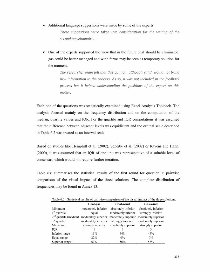
235

Additional language suggestions were made by some of the experts.

These suggestions were taken into consideration for the writing of the

second questionnaire.

One of the experts supported the view that in the future coal should be eliminated,

gas could be better managed and wind farms may be seen as temporary solution for

the moment.

The researcher team felt that this opinion, although valid, would not bring

new information to the process. As so, it was not included in the feedback

process but it helped understanding the positions of the expert on this

matter.

Each one of the questions was statistically examined using Excel Analysis Toolpack. The

analysis focused mainly on the frequency distribution and on the computation of the

median, quartile values and IQR. For the quartile and IQR computations it was assumed

that the difference between adjacent levels was equidistant and the ordinal scale described

in Table 6.2 was treated as an interval scale.

Based on studies like Hemphill et al. (2002), Scheibe et al. (2002) or Rayens and Hahn,

(2000), it was assumed that an IQR of one unit was representative of a suitable level of

consensus, which would not require further iteration.

Table 6.6 summarises the statistical results of the first round for question 1: pairwise

comparison of the visual impact of the three solutions. The complete distribution of

frequencies may be found in Annex 13.

Table 6.6- Statistical results of pairwise comparison of the visual impact of the three solutions. Coal-gas Coal-wind Gas-wind Minimum moderately inferior absolutely inferior absolutely inferior 1st quartile equal moderately inferior strongly inferior 2nd quartile (median) moderately superior moderately superior moderately superior 3rd quartile moderately superior strongly superior moderately superior Maximum strongly superior absolutely superior strongly superior IQR 1 3 3 Inferior range 11% 44% 44% Equal range 22% 0% 0% Superior range 67% 56% 56%

236

Consensus was achieved for the comparison of the visual impact of coal and natural gas

power stations. The results revealed that more than 50% of the experts chose the same

category: “moderately superior”, followed by “equal” with 22% and “moderately inferior”

with 11%.

The comparison of coal and gas solutions with wind solution, demonstrated considerable

less agreement. The IQR was equal to 3 and the histogram clearly shows that the responses

are spread out through all categories.

Even aggregating the related categories consensus is far from being achieved. The results

showed that 44% of the experts believe that the visual impact of the coal or gas solutions is

superior to the visual impact of the wind solution. On the opposite about 56% of the

experts think that the visual impact of the wind solution is superior to the visual impact of

both coal and gas solutions.


comparison of the noise level of the three solutions. The complete distribution of


Table 6.7- Statistical results of pairwise comparison of the noise level of the three solutions.

Coal-gas Coal-wind Gas-wind Minimum equal strongly inferior strongly inferior 1st quartile equal moderately inferior moderately inferior 2nd quartile (median) equal moderately inferior moderately inferior 3rd quartile equal moderately superior equal Maximum strongly superior moderately superior moderately superior IQR 0 2 1 Inferior range 0% 67% 67% Equal range 78% 0% 11% Superior range 22% 33% 22%

There seems to exist more consensus in what concerns the pairwise comparison of the

noise level of the three solutions. High consensus was achieved for the comparison of the

noise impact of coal and natural gas power stations. The results revealed that about 78% of

the experts chose the category. “equal”. Only 22% of the experts chose categories of the

“superior” range.

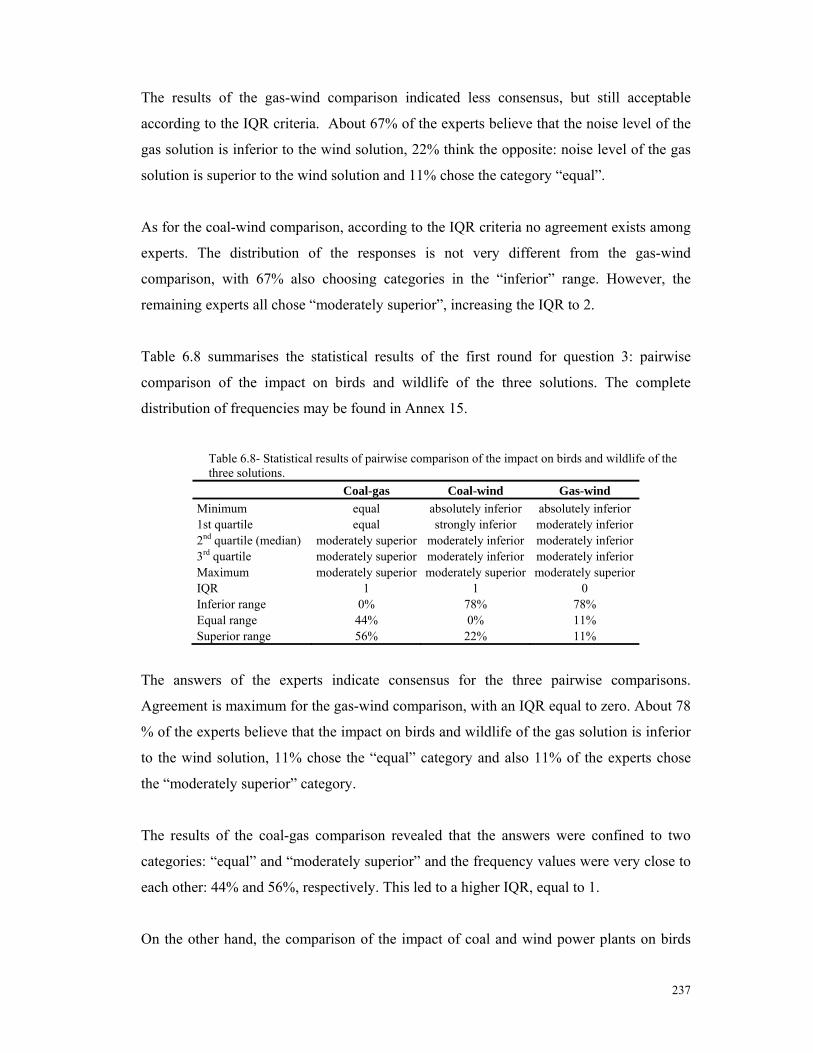
237

The results of the gas-wind comparison indicated less consensus, but still acceptable

according to the IQR criteria. About 67% of the experts believe that the noise level of the

gas solution is inferior to the wind solution, 22% think the opposite: noise level of the gas

solution is superior to the wind solution and 11% chose the category “equal”.

As for the coal-wind comparison, according to the IQR criteria no agreement exists among

experts. The distribution of the responses is not very different from the gas-wind

comparison, with 67% also choosing categories in the “inferior” range. However, the

remaining experts all chose “moderately superior”, increasing the IQR to 2.


comparison of the impact on birds and wildlife of the three solutions. The complete

distribution of frequencies may be found in Annex 15.

Table 6.8- Statistical results of pairwise comparison of the impact on birds and wildlife of the three solutions.

Coal-gas Coal-wind Gas-wind Minimum equal absolutely inferior absolutely inferior 1st quartile equal strongly inferior moderately inferior 2nd quartile (median) moderately superior moderately inferior moderately inferior 3rd quartile moderately superior moderately inferior moderately inferior Maximum moderately superior moderately superior moderately superior IQR 1 1 0 Inferior range 0% 78% 78% Equal range 44% 0% 11% Superior range 56% 22% 11%

The answers of the experts indicate consensus for the three pairwise comparisons.

Agreement is maximum for the gas-wind comparison, with an IQR equal to zero. About 78

% of the experts believe that the impact on birds and wildlife of the gas solution is inferior

to the wind solution, 11% chose the “equal” category and also 11% of the experts chose

the “moderately superior” category.

The results of the coal-gas comparison revealed that the answers were confined to two

categories: “equal” and “moderately superior” and the frequency values were very close to

each other: 44% and 56%, respectively. This led to a higher IQR, equal to 1.

On the other hand, the comparison of the impact of coal and wind power plants on birds

238

and wildlife indicate the opinions of experts were spread across four categories. However,

44% of the answers were in the “moderately inferior” category and a total of 78% of the

answers ranged in the inferior scope. The remaining 22% of the experts think that the

impact on birds and wildlife of the coal solution is “moderately superior” to the wind

solution. The IQR was again equal to 1.


comparison of the social acceptance of the solutions. The complete distribution of


Table 6.9- Statistical results of pairwise comparison of the social acceptance of the solutions. Coal-gas Coal-wind Minimum very strongly inferior absolutely inferior1st quartile strongly inferior very strongly inferior2nd quartile (median) moderately inferior very strongly inferior3rd quartile moderately inferior moderately inferior Maximum strongly superior absolutely superior IQR 1 2 Inferior range 78% 89% Equal range 11% 0% Superior range 11% 11%

Once more consensus was achieved for the comparison of the social acceptance of the coal

and natural gas solutions. The distribution of the responses indicates that about 78% of the

experts think that the social acceptance of the coal solution is inferior to the gas solution,

11% believes that it is the same and the remaining 11% chose the “strongly superior”

category.

The results showed considerable less agreement in what concerns the coal wind

comparison. Although 89% of the experts chose responses from the inferior range, the IQR

was equal to 2. In fact, the distribution of the frequencies showed that the answers were

spread across five categories and all of them with a frequency of response less than 34%.

In the inferior range, the responses varied from “absolutely inferior” to “moderately

inferior” and the IQR reflected this dispersion.

Due to a mistake, detected after sending of the questionnaires, no gas-wind comparison

was conducted. This question was addressed only on the second round.

239

The second part of the questionnaire focused on the pairwise comparison of the social

criteria. Table 6.10 summarises the statistical results of the first round. The complete

distribution of frequencies may be found in Annex 17.

Table 6.10- Statistical results of pairwise comparison of the social criteria. VI-NL VI-BW VI-SA NL-BW NL-SA BW-SA

Minimum absolutely inferior

absolutely inferior

very strongly inferior absolutely inferior strongly inferior strongly

inferior

1st quartile moderately inferior

strongly inferior

*strongly to moderately inferior



moderately inferior

2nd quartile (median)

moderately inferior

moderately inferior moderately inferior *moderately

inferior to equal *moderately

inferior to equal equal

3rd quartile moderately inferior

moderately superior equal strongly superior moderately superior equal

Maximum strongly superior

strongly superior equal strongly superior strongly superior moderately

superior IQR 0 3 1.25 3.25 2.25 1 Inferior range 78% 67% 67% 44.4% 44.4% 44.4% Equal range 0% 0% 33% 11.1% 11.1% 33.4% Superior range 22% 33% 33% 44.4% 44.4% 22.2%

* The computation of these quartile values led to non integer values. VI-Visual impact; NL- Noise level; SA- Social acceptance; BW- Impact on birds and wildlife.

The answers of the experts indicate consensus for the pairwise comparison of visual impact

with noise level. About 78% of the experts chose answers in the inferior range and the

remaining 22% chose the “strongly superior” category. Consensus was also achieved for

the comparison of impact on birds and wildlife and social acceptance, with an IQR equal to

1. However, the opinions of the experts were spread across more categories ranging from

“strongly inferior” to ”moderately superior”. For all the other pairwise comparisons, the

responses obtained from the experts did not lead to agreement. The IQR was higher than 1

and the frequency distribution shows that the responses were spread across the different

categories and ranges, reflecting the high subjectivity of the analysis.

The third part of the questionnaire focused on the experts’ willingness to pay for a

reduction in pollution levels. Table 6.11 summarises the statistical results of the first round.

The complete distribution of frequencies may be found in Annex 18.

The results showed no agreement in regard to this question. Most of the experts indicate

that they are willing to increase their electricity bill by more than 10%. However, the

distribution of the frequencies showed that the answers were spread across the four

categories, with the IQR reflecting this dispersion.

240

Table 6.11- Statistical results of pairwise comparison of the “willingness to pay” question.

ValueMinimum 0% 1st quartile up to 5% 2nd quartile (median) from 6 to 10% 3rd quartile more than 10%Maximum more than 10%IQR 20% 22.2% Up to 5% 22.2%From 6 to 10% 11.2% More than 10% 44.4%

Table 6.12 presents a summary of the results of all the questions for the first round of the

Delphi process.

Table 6.12 Summary of the results of the 1st round.

Question IQR Consensus 1. Visual impact

Coal-gas 1 Yes Coal-wind 3 No Gas-Wind 3 No

2. Noise level Coal-gas 0 Yes Coal-wind 2 No Gas-Wind 1 Yes

3. Impact on birds and wildlife Coal-gas 1 Yes Coal-wind 1 Yes Gas-Wind 0 Yes

4. Social acceptance Coal-gas 1 Yes Coal-wind 2 No

5. Social criteria Visual impact-noise level 0 Yes Visual impact-birds and wildlife 3 No Visual impact-social acceptance 1.25 No Noise level-impact on birds and wildlife 3.25 No Noise level-social acceptance 2.25 No Impact on birds and wildlife-social acceptance 1 Yes

6. Increase in electricity bill 2 No

The application of the IQR equal to 1 principle produced adequate consensus for 9 of the

18 questions. These questions did not required further iteration and were not included in

the second round of the questionnaire.

The results from pairwise comparison of the three solutions indicate that visual impact is

241

the criteria with maximum disagreement among experts. As mentioned previously this is

not a completely unexpected result, with the high subjectivity of this criterion easily

leading to divergent opinions. The position of the experts in regard to the impact on birds

and wildlife is quite consensual, and most of the expert seem to agree that the impact of

coal or gas power plants is moderately inferior to the impact of wind power plants.

The pairwise comparison of the social criteria revealed increased difficulties in obtaining

consensus. Once more, this is probably due to the subjectivity of the comparison and

several experts reported the difficulty of the process. However, it is interesting to note that

the idea that visual impact is the least important of the criteria considered seems to be

consensual, corroborating the opinions collected during the first stage of semi-structured

interviews.

As for the willingness to pay more for a better environment, no consensus was achieved,

requiring a further Delphi round. However, comparing the results with the European

Commission survey “Attitude towards energy”, it appears that expert may be willing to pay

more than the average population. This is also not a surprising result, as the European

Commission (2006) states “Education indeed seems essential in order to recognize and

face the new energy related challenges”. Our group of experts is composed of academic

staff and may be more “open-minded” with regard to clean electricity production even

when cost implications are involved.

VI.5.3 Second questionnaire

The second questionnaire, sent to experts in January 2007, may be found in Annex 19. This

questionnaire followed the same structure as the first one, asking the experts to assume the

need to increase the available power in about 1000 MW. It included again a description of

the three possible solutions. No changes were made on the characterisation of the coal and

gas solutions. However, the characterisation of the wind solution was changed according to

the technical comments received during the first round. Additionally, a picture from a more

recent wind farm replaced the previous one.

242

Wind solution Description 180 new wind farms, with total installed capacity equal to 3800 MW. Placement Spread across the country, but with some particular relevance in the inland North

hills. Characteristics Each wind farm will have between 8 and 10 turbines, about 65 m high and may

occupy an area of about 25 ha (0.25 km2). Examples Presently there are about 1000 turbines operating in the mainland, some examples

may be seen in Marão, Açor, Barroso among many others.

The other comments, described in section VI.5.2 were also included in the new

questionnaire, namely:

For the wind solution the installed power must be much higher than the average power needed. Due to wind fluctuations and intermittency, the average available power for electricity production on the wind solution is much lower than the installed power, which does not happen with either the coal or the gas solution. The visual impact of a wind farm may be superior to the other solutions. However, some may consider this a positive impact because it represents an image of clean energy production.

The questionnaire also included a simple description of the statistical concepts used for

describing the results from the first round (quartile values):

1st quartile: 25% of the responses were equal or less than the category presented. 2nd quartile (median): 50% of the responses were equal or less than the category presented. 3rd quartile: 75% of the responses were equal or less than the category presented.

Together with the additional information, questions for which round one did not produce

an acceptable level of agreement were formulated in this second questionnaire. The

experts’ panel was presented with a summary of statistical results along with their original

response to round one as feedback. Based on this information, the experts could maintain

or revise their initial response. For example, question 1a) was formulated as follows:

The visual impact of the coal solution is to the wind solution.

Results from the first round: 1st quartile: “4-moderately inferior” 2nd quartile (median): “6-moderately superior” 3rd quartile: “7-very strongly superior” Your answer to first round was:

As stated before, the ordinal scale presented to the panel members was converted to an interval

scale for the statically analysis. In order to better understand the results from the first round and

to make clear the assumption of equidistance between response categories, in the second round

243

this numerical scale was presented associating to each category a rank order between 1 and 9.

This second round reduced the number of questions from the original 18 (in the first round) to

10. However, the complexity of the process was increased because the experts had now to

analyse the alterations and comments made, along with the statistical results of the first round.

To facilitate the experts’ job and to reduce the answering time, the second questionnaire

distinguished this new information from the remaining text. The experts could easily recognise

the new information, because it was written in a different colour and the statistical results were

presented in boxes next to the respective question.

The process began in the second week of January 2007 and the first round was concluded in the

last week of February 2007.

VI.5.4 Results of the second round

The questionnaire was sent to the 9 experts that previously answered the first questionnaire

and all of them completed it. Once more, it was necessary to encourage involvement

through electronic and telephone reminders. The process lasted for a longer period than the

first round, which may be associated with the complexity of the analysis and some

weariness of the participants.

During the second round two additional comments were received, both related to visual

impact. These experts believed that the interpretation of visual impact was not

straightforward. Some experts might answer on the basis of the direct impact of wind

power plants on the landscape; and others might be influenced by the public opinion’s

positive image of wind power.

Similarly to the 1st round, each one of the questions was statistically examined using Excel

AnalysisToolpack. Along with statistical measures, the percentage change of the responses

was also computed to evaluate the stability of the process. Following Schebe et al. (2002),

a 15% change level or less indicated stability.

Table 6.13 summarises the statistical results of the second round for question 1: pairwise

comparison of the visual impact of coal and wind solutions and comparison of the visual

244

impact of gas and wind solutions. The complete distribution of frequencies and the stability

measurement computations may be found in Annex 20.

Table 6.13- Statistical results of pairwise comparison of the visual impact of the solutions (2nd round).

Coal-wind Gas-wind Minimum 1. absolutely inferior 1. absolutely inferior 1st quartile 4. moderately inferior 3. moderately inferior2nd quartile (median) 6. moderately superior 6. moderately superior 3rd quartile 6. moderately superior 6. moderately superior Maximum 7. strongly superior 6. moderately superior IQR 2 3Inferior range 44% 44% Equal range 0% 0% Superior range 56% 56% Change 22% 11%

Once more consensus was not achieved for the comparison of the visual impact of wind

plants with either coal or gas power plants. Although achieving a reduction of the IQR for

the coal-wind comparison, the experts are still divided about this subject. For gas-wind

comparison, the IQR remains unchanged and stability seems to have been reached,

probably due to the resistance to opinion change. For coal-wind comparison, the values

indicate no stability, however only a few changes of category in the superior range were

obtained showing a tendency to centralise in less extreme positions.

Table 6.14 summarises the statistical results of the second round for question 2: pairwise

comparison of the noise level of coal and wind solutions. The complete distribution of

frequencies and the stability measurement computations may be found in Annex 21.

Table 6.14- Statistical results of pairwise comparison of the noise level of the solutions (2nd round).

Coal-wind Minimum 3. strongly inferior1st quartile 4. moderately inferior 2nd quartile (median) 4. moderately inferior 3rd quartile 4. moderately superiorMaximum 4. moderately superiorIQR 2 Inferior range 67% Equal range 0% Superior range 33% Change 11%

245

The IQR range remains equal to 2 and frequency distribution indicates that most of the

experts still concentrate on the inferior range with minor changes on the chosen category.

These small changes indicate that the distribution may be considered stable.


comparison of the social acceptance of coal and wind solutions and pairwise comparison of

the social acceptance of gas and wind solutions. The complete distribution of frequencies

and the stability measurement computations may be found in Annex 22.

Table 6.15- Statistical results of pairwise comparison of the social acceptance of the solutions (2nd round).

Coal-wind Gas-wind Minimum 1. absolutely inferior 3. strongly inferior 1st quartile 1. absolutely inferior 3. strongly inferior 2nd quartile (median) 2. very strongly inferior 4. moderately inferior 3rd quartile 3. strongly inferior 4. moderately inferior Maximum 4. moderately inferior 4. moderately inferior IQR 2 1 Inferior range 100% 100% Equal range 0% 0% Superior range 0% 0% Change 22% --

High consensus was achieved in the comparison of the social acceptance of natural gas and

wind solutions. The distribution of the responses indicates that all the experts think that the

social acceptance of the gas solution is inferior to the wind solution, 56% believe that it is

“moderately inferior” and the remaining 44% chose the “strongly inferior” category.

The coal-wind comparison, although aggregating all the answers in the inferior range, still

presents an IQR equal to 2. The distribution of frequencies showed that the answers were

spread across the four inferior categories and the IQR reflected this dispersion. Once more,

stability seems not to be reached. However, also in this case only minor changes of

category in the inferior range were observed.

The second part of the questionnaire focused on the pairwise comparison of the social

criteria. Table 6.16 summarises the statistical results of the first round. The complete

distribution of frequencies and the stability measurement computations may be found in

Annex 23.

246

Table 6.16- Statistical results of pairwise comparison of the social criteria (2nd round). VI-BW VI-SA NL-BW NL-SA

Minimum 2. very strongly inferior

2. very strongly inferior

2. very strongly inferior 3. strongly inferior

1st quartile 3. strongly inferior 3. strongly inferior 3.75 strongly to moderately inferior* 3. strongly inferior

2nd quartile (median)

4. moderately inferior


4.5 moderately inferior to equal*


3rd quartile 6. moderately superior


6. moderately superior

6. moderately superior

Maximum 7. strongly superior 5. equal 7. strongly superior 7. strongly superior IQR 3 1 2.25 3 Inferior range 56% 78% 44.4% 56% Equal range 0% 22% 11.2% 11% Superior range 44% 0% 44.4% 33% Change 11% 11% 33% 11%

* The computation of these quartile values led to non integer values. VI-Visual impact; NL- Noise level; SA- Social acceptance; BW- Impact on birds and wildlife.

The answers of the experts indicate consensus for the pairwise comparison of visual with

social acceptance. About 78% of the experts chose answers in the inferior range and the

remaining 22% chose the “equal” category.

For the remaining questions IQR remains high. With the exception of the pairwise

comparison of noise level with the impact on birds and wildlife, stability seems to have

been reached with an unconsensual distribution of opinions. The noise level - impact on

birds and wildlife comparison presented a tendency to centralise more extreme solutions,

which was reflected on the high percentage of change.

The third part of the questionnaire focused on the experts’ willingness to contribute

financially to a decrease in pollution levels. Table 6.17 summarises the statistical results of

the second round. The complete distribution of frequencies and the stability measurement

computations may be found in Annex 24.

The results showed again no agreement in relation to this question. The results indicates

that about 45% of the experts are not willing to increase their electricity bill or only accept

a 5% increase to contribute to a decrease in pollution levels. However, the most frequently

chosen category was “more than 10%”, once more showing the wide range of opinions on

this matter. The distribution of frequencies showed that the answers were spread across the

four categories, with the IQR reflecting this dispersion. Stability was reached with no

expert changing opinion from one round to the other.

247

Table 6.17- Statistical results of pairwise comparison of the “willingness to pay” question (2nd round).

ValueMinimum 0% 1st quartile up to 5% 2nd quartile (median) from 6 to 10% 3rd quartile more than 10%Maximum more than 10%IQR 20% 22.2% Up to 5% 22.2%From 6 to 10% 11.2% More than 10% 44.4% Change 0%

Table 6.18 presents a summary of the results of all the questions for the second round of

the Delphi process.

Table 6.18- Summary of the results of the 2nd round.

Question IQR Consensus Stability Relaxed consensus1

1. Visual impact Coal-wind 2 No No No Gas-Wind 3 No Yes No

2. Noise level Coal-wind 2 No Yes Yes

3. Social acceptance Coal-wind 2 No No Yes Gas-wind 1 Yes -- Yes

5. Social criteria Visual impact-birds and wildlife 3 No Yes No Visual impact-social acceptance 1 Yes Yes Yes Noise level-impact on birds and wildlife 2,25 No No No Noise level-social acceptance 3 No Yes No

6. Increase in electricity bill 2 No Yes No 1 Assuming consensus for questions with IQR=2 and more than 60% of the answers in one range (inferior, equal or superior).

For three questions stability was not achieved. For all of them there was an obvious

tendency to centralise more extreme positions, however this lack of stability was only due

to minor changes of category with no changes in range occurring. Most of the questions of

the second round achieved stability but not consensus, meaning that the experts opinions

are wide-ranging and some resistance exists on moving to centralisation. Even when the

relaxed consensus was assumed, only four of the 10 questions could be considered

consensual.

It is not easy to reach consensus for the issues in question and it is the researcher’s belief

248

that due to the complexity and subjectivity of the theme a third iteration would be unlikely

to bring new valuable information to the model. It was however possible to achieve

consensus in 12 of the 19 questions. It is also important to keep in mind that the group of

experts consisted of only nine persons, and as so extreme answers or changes on even just

one or two expert responses can have important effects on the statistical results and may

influence the decision of consensus or stability92. For larger groups, if there is no

agreement Hobbs and Meier’s (2003) suggestion may be followed, of using cluster

analysis or factor analysis to analyse the positions of various stakeholders.

As Hobbs and Meier (2003) state, one should expect significant differences among

individuals concerning their values on energy planning alternatives. These authors argue

that consensus may be very difficult or even unachievable, yet often the search for

consensus will establish at least some common ground. Based on this, it seemed reasonable

to proceed with the study, applying the results obtained to an exploratory model to develop

a methodology to incorporate non quantitative aspects in the electric planning process.

This group of experts should be seen as a pilot group; nevertheless even if a broader group

of social agents is consulted difficulties and divergence of opinions on the subject are

always to be expected. On a more general level, the study would greatly benefit from

increasing the number of experts consulted and from the inclusion of other social groups.

This would bring more views to the discussion and would make the statistical analysis less

sensitive to individual extreme positions. The involvement of central planners in the

Delphi study would bring considerable advantages to the process, contributing for the

definition of the social criteria more relevant for the Portuguese society and increasing the

number of experts participating in the study.

VI.6 Determination of weights for the electricity generation options

This phase of the research combines the information obtained from the Delphi process with

AHP, in order to convert pairwise comparison of the elements of the hierarchical structure

in an overall social index, allowing for the ranking of the alternative ways of meeting the

demand for electricity. The pairwise comparisons of each expert were used as input for the

SuperDecisions software using the scale presented in Table 6.2 associated with a numerical

92 For example for the pairwise comparison of the visual impact of coal and wind solutions if two of the experts holding position “moderately inferior” would change their position to “equal” the IQR would be equal to one and consensus could be assumed.

249

score as presented in Table 6.19.

Table 6.19- Scale preferences with numerical score

Score Pairwise evaluation 9 Absolutely superior 7 Very strongly superior 5 Strongly superior 3 Moderately superior 1 Equal

1/3, 1/7, 1/5, 1/3 Reciprocal values

The consistency of each comparison matrix was tested and the relative weights of the

elements on each level were computed for each expert.

As the consistency ratio is above 10% for some of the resulting matrixes, only the relative

scores of matrixes passing the consistency test were included in the aggregation process.

Thus:

the relative weights of the alternatives with respect to noise are based on 8 experts’

points of view;

the relative weights of the alternatives with respect to impact on birds and wildlife

and social acceptance aggregate the opinions of 5 experts; and

for visual impact only 4 experts provided judgments passing the consistency test.

The relative weights of the four criteria aggregate opinions from 6 experts.

The group view was represented by the aggregation of each individual’s resulting

priorities. Forman and Peniwati (1998) argued that although this aggregation may be

computed using either a geometric or arithmetic mean, the geometric mean is more

consistent with the meaning of both judgments and priorities in AHP. In fact, studies such

as Hon et al. (2005), Wu et al. (2007) or Banuls and Salmeron (2006), resource also to the

the geometric mean method. Tables 6.20 and 6.21 give the aggregated comparison matrix

for the criteria and for the alternatives under each criterion using the geometric mean for

the aggregation of the experts’ opinions into the final judgement 93.

The priority vector ranking of criteria with respect to the general goal indicates that social

acceptance ranked first followed by impact on birds and wildlife. All these criteria reflect

negative aspects for society. For the sake of the consistency of the analysis, social

93 Values obtained with the software package Super Decisions.

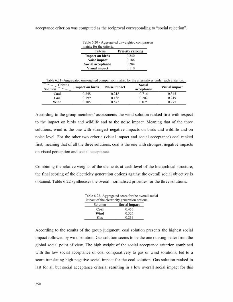
250

acceptance criterion was computed as the reciprocal corresponding to “social rejection”.

Table 6.20 - Aggregated unweighted comparison matrix for the criteria. Criteria Priority ranking

Impact on birds 0.240 Noise impact 0.186

Social acceptance 0.284 Visual impact 0.110

Table 6.21- Aggregated unweighted comparison matrix for the alternatives under each criterion.

Criteria Solution Impact on birds Noise impact Social

acceptance Visual impact

Coal 0.248 0.218 0.716 0.345 Gas 0.199 0.186 0.202 0.219

Wind 0.385 0.542 0.075 0.275

According to the group members’ assessments the wind solution ranked first with respect

to the impact on birds and wildlife and to the noise impact. Meaning that of the three

solutions, wind is the one with strongest negative impacts on birds and wildlife and on

noise level. For the other two criteria (visual impact and social acceptance) coal ranked

first, meaning that of all the three solutions, coal is the one with strongest negative impacts

on visual perception and social acceptance.

Combining the relative weights of the elements at each level of the hierarchical structure,

the final scoring of the electricity generation options against the overall social objective is

obtained. Table 6.22 synthesises the overall normalised priorities for the three solutions.

Table 6.22- Aggregated score for the overall social impact of the electricity generation options.

Solution Social impact Coal 0.455Wind 0.326 Gas 0.219

According to the results of the group judgment, coal solution presents the highest social

impact followed by wind solution. Gas solution seems to be the one ranking better from the

global social point of view. The high weight of the social acceptance criterion combined

with the low social acceptance of coal comparatively to gas or wind solutions, led to a

score translating high negative social impact for the coal solution. Gas solution ranked in

last for all but social acceptance criteria, resulting in a low overall social impact for this

251

option.

VI.7 Discussion of the results

The prioritisation process of the different electricity generation options based on their

social impact is a complex problem that involves subjective value judgments. An

evaluation method combining AHP and Delphi method was adopted. The hierarchical

structure enabled the relevant social criteria to be isolated, allowing the clear evaluation of

each alternative against each criterion. The Delphi panel of experts allocated scores to each

level of the hierarchical structure with the final aim of obtaining an overall social index of

the alternatives.

The experts revealed some difficulties in translating their opinions using a scale for

comparing alternatives and on the generalisation of their opinions on each of the

generation alternatives and criteria. The comparison of the wind solution with both gas and

coal solutions with respect to their visual impact, was particularly difficult due not only to

the subjectivity of the subject but also due to the different interpretations of the concept:

some of experts based their answers on direct impact of wind turbines on the landscape and

others associated wind farms with clean energy production and perceived the visual impact

as positive. It was also not possible to achieve consensus when assessing the importance

of some of the criteria to the overall social ranking of the alternatives. Even in the second

round, few changes occurred and most of the experts showed resistance to moving to

centralisation.

After collecting the data, the consistency of the responses of each expert was analysed.

Due to the complexity of the subject studies like Linares and Romero (2002), assumed that

a 20% CR would be acceptable when assessing the importance of several criteria to the

energy planning problem in Spain. For the present study, Saaty proposed value for the CR

was imposed and the minimum CR was set equal to 0.1 (Kablan, 2004). Only the experts’

matrixes complying with this condition were included in the final aggregation.

It should be highlighted that the difficulty on reaching consensus and consistent results is

not a completely unexpected result. As Hobbs and Meier (2003) pointed out, trading off

attributes often involves conflicting, strongly held values, leading to unstable weights.

252

Based on their experience, the authors state that many energy planners and decision makers

are uncomfortable with tradeoff questions, therefore it is important to check consistency.

Also, the broad diversity of interests and values of the decision makers makes consensus

very difficult to achieve in the energy planning process.

Regardless of these difficulties, the research succeeded in proposing and testing a

framework to deal with the non quantitative aspects of the energy planning process. It was

possible to select and encourage a group of experts to participate on the research as a pilot

group building an exploratory model to integrate their individual opinions. From the

information collected an overall social index was assigned to each electricity generation

option.

According to AHP results, the rank of gas solution was the first in the order of priority,

most probably because it represents a compromise solution. It is seen as an electricity

generation solution with low environmental problems, which increases its social

acceptance over coal. It has also reduced impacts on wildlife specially when compared to

wind power, and lower visual and noise impact than both other alternatives. Coal ranks in

last, mainly due to the reduced social acceptance of this alternative. The impact on birds

and wildlife and the noise impact are the most severe effects reported for wind power

comparatively to both coal and gas solutions. The next section of this chapter combines

this social evaluation with the environmental and economic evaluations of the the NLEPM

described in Chapter V, resulting in a new Integrated Electricity Planning Model (IEPM).

VI.8 Incorporating the social index into the electricity planning model

Figure 6.5 outlines the IEPM, including the input information, output results and the

aggregation of information.

The input information for the problem includes:

the criteria identified and assumed to be relevant for the evaluation process;

the acceptable plans drawn from the NLEPM and characterised by the cost, CO2

levels, external energy dependency and associated capacity expansion;

253

the basis for the Delphi survey: panel of experts and questionnaires.

Delphi analysis

AHP

Acceptable plans

Cost

CO2

Capacity expansion

Data

Social impact

Delphi survey

Panel of experts

Questionnaire

Results

Social ranking

NLEPM

Delphi analysis

AHP

Acceptable plans

Cost

CO2

Capacity expansion

Data

Social impact

Delphi survey

Panel of experts

Questionnaire

Results

Social ranking

NLEPM

Figure 6.5- Schematic resume of the IEPM.

AHP and Delphi techniques are used for the analysis of the input to the model and the final

result is a social ranking for each electricity plan. In order to obtain a final ranking of the

available solutions, the overall social scores of the three alternatives must be aggregated by

means of a mathematical algorithm. The aim is to get a final index for each possible plan,

combining more than one of the available electricity generation technologies. For this the

weights were aggregated using an additive function.

This additive function assumes that the weights assigned to each electricity generation

option are constants and satisfy the additive independence, i.e. these weights do not depend

on the relative levels of each option. This additive value model offers a simple way of

evaluating multiattribute alternatives. This simplicity makes it widely used in energy

planning and policy, as described by Hobbs and Meier (2003).

Equation 6.6 presents the computation of the average social index (ASI) for each electricity

plan derived from the NLEPM, depending on the installed power of each electricity

generation option and on the weights derived from the AHP.

254

( ) ( ) ( )

( )∑∑∑∑+++++

+++++=

t3t9t2t5t1t4t

windt

3t9tgast

2t5tcoalt

1t4t

IPIPIPIPIPIP

WIPIPWIPIPWIPIPASI (6.6)

Where Wcoal, Wgas, Wwind, represent the overall normalised weights for the coal, gas and

wind solutions, described in table 6.22.

From the NLEPM resulted an emission-cost tradeoff curve. This curve is described by

discrete points, each one representing an optimal strategy for the electricity sector in the

next 10 years. However, as mentioned before the non optimal solutions may not be easy to

discard. Decision makers may not be willing to reject some plan that is not significantly

worse than the mathematical optimal and may be more interesting from the social point of

view.

The inclusion of the social index on the electricity planning process acknowledges the

existence of alternative electricity plans drawn directly from the optimisation process and

additional plans that although not optimal from the mathematical point of view may be

socially more interesting. To illustrate the process a set of possible plans were chosen,

taking into consideration that the average annual CO2 level for the power plants included in

the model could not exceed 20 Mt (Kyoto protocol target): the Solutions described in Table

5.16 were used, representing plans not necessarily belonging to the Pareto front.

Table 6.23 presents again these plans along with the respective computed ASI.

Table 6.23- Possible electricity plans obtained from NLEPM. NLS4 NLS4.1 NLS5 NL5.1 Comments Pareto

solution IP3a,2012

≥6500 Pareto

solution IP3a,2012

≥6500

Tota

l in

stal

led

pow

er

(MW

)

Coal (new) 2400 600 Coal (existing) 1820 1820 1820 1820 Natural gas (new) 5040 1860 5110 3720 Natural gas (existing) 2916 2916 2916 2916 Wind (new) 3225 6514 3225 6500 Wind (existing) 1515 1515 1515 1515 Large hydro 5805 5805 5805 5805 NWSRP 3245 3245 3245 3245 Total 23566 26075 23636 26121

Share of RES (%) 39 45 39 46 External dependency (%) 65 58 65 57 Cost (€/MWh) 33.627 34.961 34.365 36.950 CO2 (ton/MWh) 0.379 0.379 0.332 0.332 ASI 0.284 0.328 0.284 0.303

255

Some factors condition the range of ASI94 values obtained:

The renewable constraint imposes a minimum amount of wind power in the

system. Even for plans with lower installed wind power, this technology still

represents about 20% of the total installed power in the system. For large wind

scenarios (solutions NLS4.1 and NLS5.1) this share reaches a little more than

30%, meaning that the maximum difference between plans is only about 10% in

what concerns installed wind capacity.

The system already possesses substantial coal and gas power capacity, once more

diluting the effect of new entrances. For example, for NLS4 and NLS5 although

not any new coal power plants are projected, the installed coal share still represents

almost 8% of the total installed power in the system.

The Kyoto protocol, imposes maximum CO2 levels. Extreme solutions

characterised by high coal shares and that might represent plans with higher ASI

are not included in the analysis. Likewise, plans with very low CO2 levels (and

lower ASI) represent a high cost increase and may be view as academic due to the

exclusive reliance on new CCGT, hydro and SRP (NLS7 or NLS8 describe din

Table 5.15 for example).

The differences on the ASI seem to be mainly influenced by the installed power of

coal power plants.

Plan NLS4.1 presents the worst outcome from society’s point of view, because of

the high values for the installed wind and coal power and lower installed power of

gas plants.

Plans NLS4 and NLS5 present the lower ASI due to the reduced share of coal and

high share of gas power plants.

Combining the results of the optimisation procedures with the data collected in the

participative process, it will be possible to present the decision maker with a selected 94 The ASI ranges between 0.280 (NLS7) and 0.357 (NLS0) for the plans presented in Table 5.15.

256

number of feasible electricity generation plans characterised by the mix of technologies,

total cost, total CO2 emissions, ASI and external dependency. For example, with respect to

the plans described in Table 6.23, the results reveal that it will be possible to achieve

average CO2 emissions equal to 20 Mton/year at a minimal cost of 33.6 €/MWh, investing

mainly on new natural gas power plants (Solution NLS4). As natural gas is a socially well

accepted solution, the social impact of this strategy should be low95 but the external

dependency of the electricity generation sector will remain high. If the decision maker is

willing to increase cost by about 4% (Solution NLS4.1), it will be possible to keep CO2

emissions at the same level and the external dependency of the electricity production sector

may be reduced by 7%. Also, a more equilibrated mix between coal and natural gas may be

achieved resulting in considerable advantages from the security of supply point of view.

However, as this strategy requires less natural gas power plants and additional investments

in new coal and wind power plants, the ASI of NLS4.1 is higher than the value obtained

for the NLS4 solution.

This analysis allows the decision maker to recognise the differences between possible

electricity generation alternatives and foresee their estimated impacts. The final selection

of an electricity strategy for the future depends on the priority that the decision maker

chooses to assign to each one of the objectives considered.

VI.9 Conclusions

The complex nature of different generation options has been highlighted by this analysis.

The combination of Delphi and AHP methodologies was used to illustrate a possible

process of social evaluation of the future electricity plans assigning a numerical scale to

each individual option. The process started with the identification of the relevant criteria

and the selection of the experts that participated in the process as a pilot group. The global

objective of the hierarchy process was to obtain a ranking of the three generation options

(alternatives) translating social attributes into an ASI based on the views of a group of

experts. Economic and emission criteria were already addressed with the optimisation

model. Optimal and close to optimal solutions drawn from the NLEPM were then

analysed.

95 In what concerns the four social criteria analysed: impact on birds and wild life, visual impact, noise level and social acceptance.

257

In general, the results of the Delphi analysis revealed lack of consensus among experts in

some questions. In particular, the visual impact of the wind solution comparatively to both

the coal and the gas solutions seems to be the least consensual aspect. It was also difficult

or even impossible, to reach consensus regarding the pairwise comparison of the

importance of all the criteria. However, the results seem to be stable with only few

response changes between the first and second round.

The AHP results also revealed some inconsistency, leading to the reduction on the number

of responses considered valid for each pairwise comparison. A careful analysis of the

results allowed for the computation of a numerical index characterising each generation

option from the social point of view. According to the aggregated information collected

from the experts, the best solution from the social point of view would be NLS4 or NLS5

due to the reduced share of coal and high share of gas power plants. Nevertheless, the

results must be approached with caution because they depend on the experts consulted and

on their individual judgments. If considering the individual preferences of each expert, the

rank of the options would be different from the one obtained with the aggregated weight

analysis. For example, for experts with a strong wind preference the solutions with lower

ASI would be NLS4.1 and NLS5.1.

The research included only three generation options. The results led to a high negative

social impact assigned to the coal solution, mainly due to low social acceptance. However,

the energy markets are dynamic and the social perception of each technology is highly

influenced by strong stakeholder groups and in particular media (Shackley et al., 2005).

The new clean coal technologies and the prices development may easily change this

general opinion. Likewise, the spreading of wind power plants may demonstrate that the

social impacts of this technology are more or less important than these experts assumed.

The combination of social, environmental and economic evaluations will benefit the

energy plan formulation, ensuring the robustness of the process and leading to a defensible

choice aimed at reducing conflict. A mixed model of subjectivity and objectivity is

ultimately needed for the best ranking tool (Nigim et al., 2004). The experiment conducted

revealed that the process is long and difficult. Regardless of these implementation

difficulties, based on the opinions of a group of experts, the model recognises the overall

social impact of each electricity generation option, identifies their major reported impacts

258

and assesses the relative importance of these impacts for the society.

VI.9.1 Limitations and research requirements

The application of the model was presented through a pilot experiment, but considerable

research is still required.

In particular, the research must go beyond the pilot experiment by the inclusion of possible

additional social criteria and by increasing the number of participants in the questionnaire

phase. The identification and inclusion of participants representing different stakeholder

groups may add new information to the process. A broader analysis could contribute to the

identification of the major sources of concern for each stakeholder group, giving also

further insight into aspects of acceptance and critical factors for success in developing

electricity generation projects and strategic plans.

The research revealed that the responses are some times inconsistent and consensus among

experts is difficult to achieve. The process may be complemented with interviews and by

presenting the feasible plans to the experts. This may help clarify experts’ judgments and

contribute to obtaining additional insights on the electricity generation technologies in the

context of the overall electricity plan.

CHAPTER VII

INTEGRATED ELECTRICITY

PLANNING MODEL

This chapter presents the Integrated Electricity Planning Model, describing the

main steps involved in the proposed methodology for the formulation of

electricity plans.

261

VII.1 Introduction

The research presented in the previous chapters strongly emphasised the need to address

social aspects along with the economic, environmental, legal and technical factors. This

calls for the inclusion of qualitative aspects and involvement of individuals either

representing experts or stakeholders. This of course adds additional complexity to the

traditional models but it is also essential to support the energy decision process based on

more defensible assumptions.

A structured decision making process should include the definition of objectives and

measures of performance, the identification and evaluation of alternatives, and offer

choices based on a clear understanding of uncertainties and trade-offs (Failing et al., 2007).

In general, this structured decision making process is comprised of the following steps:

The identification and structuring of the problem. In this phase the decision maker

clarifies the problems and the main goals of the decision process.

The identification and characterisation of the alternatives. The information

necessary for making an informed decision is gathered together and considered.

The definition of performance measures. Based on the objectives considered the

evaluation criteria are established.

The evaluation of the alternatives. Each alternative is evaluated based on

predictions of how it will affect the performance measures.

The selection of the alternatives. This step involves addressing trade-offs among

competing objectives. At the end a preferred option is selected by the decision

maker for implementation.

From the work presented in this thesis, a structured decision making process for the

electricity power planning problem may now be outlined, combining different techniques

and involving several integrated steps. The Integrated Electricity Planning Model (IEPM)

highlights the importance of the specific technical analysis of each electricity system but

262

recognises also that energy decisions should be guided by a context that reflects economic,

environmental and social concerns. This distinct and comprehensive referential framework

is a useful instrument to distinguish and evaluate different energy strategies and plans,

thereby contributing for facilitating explicit discussion and informed decision making,

VII.2 Integrated Electricity Planning Model

Based on the models presented, the main steps of the proposed multidimensional electricity

planning process are summarised in Figure 7.1 and applied in particular to Portugal.

Energy reports, legal and technical documents

Literature review and interviews

Social

Selection of the criteria

EnvironmentalEconomic

Identification of the alternatives Data collection Characterisation of the system

EPM/NLEPM results Optimal electricity plans

Optimisation problemMathematical formulation

Selection of the experts Description of the social criteria

Social resultsRanking of the alternatives

Integrated resultsAverage social indexTotal costCO2 emissionsExternal energy dependency

Alternatives valuationDelphi and AHP formulation

Identification of the problemElectricity power planning in Portugal

Energy reports, legal and technical documents

Literature review and interviews

Social

Selection of the criteria

EnvironmentalEconomic

Identification of the alternatives Data collection Characterisation of the system

EPM/NLEPM results Optimal electricity plans

Optimisation problemMathematical formulation

Selection of the experts Description of the social criteria Selection of the experts Description of the social criteria



Integrated resultsAverage social indexTotal costCO2 emissionsExternal energy dependency





Figure 7.1- Multidimensional participatory model for electricity planning.

Step 1: Identification of the problem:

This research focused in particular on the case of electricity power planning in

Portugal. The analysis of the energy system in Portugal indicated that the electricity

generation sector is the largest consumer of primary energy, relying mainly on

imported energy sources. In addition, the high level of greenhouse gas emissions

263

(GHG) of the sector makes it an important target for CO2 mitigation.

The main goal was to identify the optimal electricity power plan for a ten year

planning period (2008-2017) in Portugal, based on the established objectives and

on the performance measures.

Step 2: Identification and characterisation of the alternatives:

This step involves the characterisation of the existing electricity system and the

identification of possible electricity generation alternatives to be added in the

future. The power plants were characterised along with the demand and all relevant

characteristics of the Portuguese electricity system. Besides collecting information

on each individual technology, the operating conditions of the entire system were

also considered.

The characterisation of the power plants included the analysis of their investment

and operating costs, CO2 emissions and characteristic curve of operation. Aspects

like the expected hydro inflows, reserve levels for the hydro storage power plants,

security of the system and legal requirements were also taken into account.

The electricity generation alternatives were explicitly defined and the electricity

plans or strategies for the future are based on a mix of these technologies. These

plans are thus implicitly defined under the mathematical formulation of the model.

Step 3: Selection of the criteria taken into consideration in the decision process.

The literature review on sustainable energy planning demonstrates the need to

integrate financial, environmental and social dimensions into the decision process.

The economic and environmental impacts (pollutant emissions) can be described

according to quantitative scales, although measured in different units. Most of the

other impacts can not be described with values directly derived from the technical

characteristics of the electricity system. The participation of the social players

becomes then essential.

264

The main criteria considered for the evaluation problem were: total present cost of

the system for the entire planning period, total CO2 emissions released during the

planning period, the Average Social Index (ASI) and external energy dependency.

Step 4: Mathematical formulation of the economic and environmental objectives.

This step involves the evaluation of all relevant costs and pollutant emissions.

Investment, O&M, fuel and emissions costs must be evaluated based on the

characteristics of each power plant and on their operating regime in each

particular electricity system. The environmental objective may involve a variety

of aspects such as, SO2, NOx, Greenhouse Gas, water consumption and

temperature changes or industrial residuals. For this particular case, CO2 was

used as a proxy for the environmental dimension of the problem.

The Portuguese electricity system was described for the ten year planning

period using mathematical functions, to specify the objectives and the

constraints. The process resulted in two optimisation problems, corresponding

to the Electricity Planning Model (EPM) and the Non-Linear Electricity

Planning Model (NLEPM).

Step 5: Computation of the quantitative results, describing possible electricity plans.

The relative merit of each plan implicitly defined in the optimisation models is

determined on the basis of its performance on the cost and CO2 criteria.

The final result of this step is the description of possible electricity plans obtained

according to quantitative criteria, which are optimal from both financial and

environmental points of view. The external dependency of the electricity sector is

also computed for each plan. In this work, these results correspond to the output of

the NLEPM or the EPM.

Step 6: Development of a methodology for addressing the social dimension of the decision

process.

265

This step involves selecting and engaging experts and/or stakeholders in the

process. The careful selection of experts and their motivation for the research area

are fundamental to ensure the success of this process. For this particular research,

university staff was selected as a pilot group.

The process comprises of defining and characterising the social criteria to be

included in the analysis. In this study four sub-criteria were used, but in a broader

study other criteria may be important, e.g. employment, impact on local

communities or health (see for example Gamboa and Munda (2007) and Cavallaro

and Ciraolo (2005)). The aim is to present a set of attributes characterising each

electricity generation option that may help to rank these from a social perspective.

Step 7: Evaluation of the possible electricity generating alternatives in the context of

social criteria.

This step involves the integration of both Delphi and Analytic Hierarchy Process

(AHP) methodologies for ranking the alternative. The process is based on the

pairwise comparison of the alternatives and of the criteria previously defined. For

this particular study, a questionnaire was written presenting the departing situation

of the Portuguese electricity system and proposing different solutions for a

marginal increase of the available power. The questionnaire was sent to experts in a

two round Delphi process. The results of the questionnaire were analysed using

AHP.

Step 8: Computation of the social impact for each electricity generation technology.

Following analysis of the questionnaire, the electricity generation technologies may

be ranked, and a social impact value may be assigned to each of these technologies.

Step 9: Integrated evaluation of the electricity plans

Electricity plans, considered optimal (or close to optimal) from both a economic

and environmental point of view, are now evaluated from a social point view. Each

generation mix is weighted with the appropriate social index of each technology,

266

resulting in the average social index (ASI). For this research, additive independence

was assumed and weights were aggregated using a linear additive function.

From the application of the outlined process, in respect of a selected number of feasible

electricity generation plans the decision maker is given cost, total CO2, ASI and external

dependency of the electricity generation sector, from which a final decision may be made.

CHAPTER VIII

CONCLUSIONS AND FUTURE WORK

This chapter summarises the main conclusions of the thesis, research

contributions and opportunities for future research.

269

VIII.1 Conclusions

Three major challenges guide energy policy at the European and Portuguese levels:

sustainability, security of supply and competitiveness. Meeting these policy objectives

calls for profound changes in the electricity power sector, through the implementation of

policies designed to address the link between energy use and environmental deterioration.

Issues such as improving energy security, local economic development, energy prices and

improvement in energy efficiency are key priorities in European policy for the energy

sector. The rising fuel prices and a growing concern for the environment have prompted

interest in using renewable energy sources (RES). The move towards renewable energy

technologies is strongly stressed in the European and Portuguese policies. Particularly

remarkable has been the development of wind power and its expected role as an electricity

generation technology.

According to Rede Eléctrica Nacional forecasts (REN, 2005), electricity demand in

Portugal is expected to grow from 52764 GWh in 2006 by a yearly figure close to 4.4% to

82070 GWh in 2016. The present electricity system is mainly based on coal, CCGT and

hydro power. The REN’s (2005) study for the electricity power sector indicates that for the

next ten years, although all the energy sources are expected to grow, the move towards

renewable energy sources will be the most significant change in the system. This will be

mainly due to the rapid growth of the wind power sector supported essentially by the

government’s policy on renewable energy.

Electricity power planning is, using the definition of Hobbs (1995) “the selection of power

generation and energy efficiency resources to meet customer demands for electricity over a

multi-decade time horizon”. The changes in the electricity sector along with the need for

sustainable development required traditional electricity planning to expand beyond pure

financial analysis and even beyond direct environmental impact analysis. The increasing

use of RES in electricity systems adds additional considerations to the traditional planning

models, in particular the need to take into account: (i) their frequent priority access to the

grid system; (ii) the impacts that technologies of variable output, such as wind energy can

have on the overall operation of the electricity system and (iii) the public attitude towards

these technologies. In addition, the central electricity planning process based on a single

decision maker is no longer acceptable and the importance of examining tradeoffs among

270

objectives is now well recognised. Considering the three dimensions of sustainable

development has gradually increased the importance of the social aspect in the decision

process. The energy planner has now the task of designing electricity strategies for the

future with the view of enhancing the financial performance of the sector while

simultaneously addressing environmental and social concerns. Thus, the planners must

deal, not only with variables that may be quantified and simulated but also with the social

impact assessment.

The electricity planning process has been addressed by a large number of authors,

proposing different approaches and methods to solve these problems. Most of these

approaches include diverse multicriteria tools, expressing each criteria in its own units, or

involving some kind of cost benefit analysis, in which environmental criteria are expressed

in economic terms. The process frequently requires the planner to work with quantitative

and qualitative information. However, continuous models like the ones from the EFOM or

MARKAL family, focus mainly on the cost and economic dimensions of the problem.

Some of the less quantifiable issues associated with the social impacts of electricity

generating activities have been covered by multicriteria methods, using well recognised

methods like the ones from the outranking family or the Analytic Hierarchy Process

(AHP), or by the economic valuation of externalities like the ExternE study. The literature

extensively debates the methods available and provides some examples of application.

Most of these examples focus on the analysis of specific technologies, on the comparison

of different power production options or on the evaluation of power generation expansion

scenarios for small systems. However, the integration of the cost, emissions and social

impact of a full scale real National electricity planning that combines multiobjective

optimisation models and models dealing with discrete alternative options, is still not fully

explored.

Several barriers which prevent renewables from being competitive and fully integrated in

the current power market have been identified. Although, renewable energies have in

general much lower emissions than conventional thermal power, past studies have

demonstrated that renewable energy technologies are not free from negative impacts, both

on the energy system itself and in regard to public acceptance. In the particular case of

wind, relevant negative impacts on the ecosystem, noise complaints and negative impacts

on the landscape were reported. In addition to these social impacts, the integration of

271

technologies of variable output like wind power in the grid poses an additional problem to

the grid management that should be addressed during the planning process. Aspects such

as the increase on reserve rudiments to deal with unexpected power output variations, the

increase on the frequency of start ups and the possible reduction of the load level of

thermal power plants are particularly relevant. Thus, the evaluation of the impact of large

scale wind power on the system’s economic and environmental performance cannot be

based on simple assumptions of substitution of electricity generation technologies and

heavily depends on the specific characteristics of the system under analysis.

In general, there appears to be a consensual view, that designing a sustainable energy plan,

is a multidisciplinary process and implies addressing and integrating technical,

environmental, economic and social dimensions. However, the integration of the relevant

dimensions of sustainable energy planning poses an important challenge to researchers.

This quest for integration is precisely the focus of this study, providing the decision makers

with a comprehensive and feasible decision support system that will assist them in

identifying optimal energy solutions. The electricity system expansion and operation

strategies should derive from an integrated planning process of the overall electricity

system, rather than by direct comparison of technologies. The study proposes a possible

model in which all these dimensions are included and fully integrated, merging

mathematical evidence based on optimisation procedures with value judgments.

Based on the literature review, a framework for electricity planning was proposed taking

into consideration the multiple objectives involved, using optimisation procedures where

possible, and incorporating value judgments in regard to social acceptability of proposed

generation plans. The research demonstrated the applicability of the new Integrated

Electricity Planning Model to the Portuguese power system planning. The system was

analysed and modelled taking into consideration both specific technical characteristics and

social impacts.

Two optimisation models, one linear and one non linear, were developed for Portugal,

combining economic and environmental objectives with legal, demand and system

constraints. The difference between the models laid mainly on the assumed impact of wind

power on the thermal power system operation. From the models, investment and

generation plans for the electricity system, which minimised costs and CO2 emissions

272

during the next 10 years, were obtained.

The models developed demonstrate the interaction between all the members of the

electricity system. A particular generation option in the system must not be analysed in

isolation and its impact on the overall electricity system must be included in the long term

planning models. For the Portuguese case, increasing penetration of wind power in the

system will have significant effects on the CCGT operation and the operating cost

reduction and environmental gains are lower than those expected on the basis of simple

substitution of technologies. In respect to the linear model these reductions in expectations

arise from the low availability of the variable energy source, wind. The non linear model

takes into consideration further impacts that large wind power will have on the power

system operating conditions. The model computes the CCGT fuel cost and CO2 emissions

as functions of the installed wind power, using evidence of the reduction of the average

load level of the CCGT plants and thus accounting for consequent loss of efficiency. The

results show that CO2 reduction is a more expensive process than what the linear model

might lead the analyst to think. For example, to reach an average yearly CO2 emission

level equal to 20Mton, close to the objective proposed for the sector in the last Portuguese

report under the Kyoto protocol96, the cost would be 1.1% higher than the one obtained

from the linear model and additional reductions become increasingly more costly. Under

the base scenario conditions, the results of the non linear continuous model indicate that

the least expensive way to achieve a CO2 level equal to 20 Mton in Portugal is a strong

investment in new CCGT and the continuous investment in new wind power plants during

the period of the plan.

To integrate social concerns into the electricity planning decision process, a combination

of Delphi and AHP methodologies for characterising and systematising experts’

preferences was used. A group of experts was invited to participate in the process of

evaluating electricity generation technologies against social criteria and a social index for

each technology was developed. These social indexes were next applied to the optimal and

close to optimal generation plans, resulting in an Average Social Index (ASI) for each of

these plans, representing the overall expected social impact of each possible electricity

generation strategy for the future. For this particular group of experts and for the analysed

96 National allocation plan (2008-2012) (available in www.iambiente.pt).

273

case, the favoured solutions are the ones with reduced share of coal and high share of gas

power plants.

The final result obtained from the Integrated Electricity Planning Model (IEPM)

application is a set of plans describing the electricity generation scheduling for the next ten

years, detailing monthly plans for the electricity production, yearly plans for the generation

capacity expansion and specifying cost, CO2 emissions, external energy dependency and

an average social index.

Figure 8.1 presents an example of feasible electricity plans obtained for Portugal. The

Figure represents the distribution of the total installed power in 2016 according to the REN

forecast and the equivalent results obtained with the IEPM for 2017, for the minimal cost

solution and for the Kyoto reference scenario (CO2=20 Mton)97 described by the financial

cost optimal solution NLS4 and the non optimal solution NLS4.1. The ASI is presented

along with the average cost and CO2 emission values and with the external dependency.

The non linear model as a part of the IEPM was used in the cases represented below.

According to the REN’s (2005) forecasts for 2016, Special Regime Producers (SRP) are

expected to represent about 35% of the total installed power in Portugal, followed by large

hydro power with a 25% share and coal and natural gas power with a 20% share each. As

the total SRP installed power is strongly constrained by the European Renewable

Directive, the results of the IEPM solutions differ from the REN scenario mainly on the

relative share of coal and natural gas sectors. The minimal financial cost solution requires a

higher reliance on coal, with no investment in natural gas power plants. On the other hand,

the imposition of maximum levels for CO2 emissions leads to a move away from coal

towards new investments in natural gas. However, it is worth recalling that the REN

scenario derives from different models, based on different assumptions and backed up by

large amounts of historical data and information that is not fully available to the researcher.

The REN scenario is presented for information purposes only and a comparative evaluation

is not appropriated. As illustrated in Figure 8.1, from the IEPM application the Decision

Maker is equipped to make an informed decision based on the cost of electricity generation

over the planning period, the total CO2 emissions from the system, the ASI of each

97 See Section V.5.1 for further detail. The Kyoto reference scenario corresponds to an average CO2 emission value equal to 0.379 ton/MWh for the 10 year planning period.

274

possible generation mix and the external dependency of any feasible electricity production

plan.

Figure 8.1- Electricity plans for the Portuguese power system.

Based on the literature review and on the illustrative application to the Portuguese case, it

would appear that the IEPM is a valuable tool for energy decision makers and for the

companies operating in the electricity market. It provides a structured methodology for the

design of future energy strategies based on sustainable development principles, allowing

for the adaptation of the proposed models to different energy systems or to changes in the

political and regulatory environment.

For regions and countries with central electricity planning, the proposed methodology

allows for the establishment of a number of electricity plans that are defensible from the

Hydro25%

Coal20%

NG20%

Wind21%

NWSRP14%

SRP35%

Electricity demand (2016) = 82 070 MWh

REN forecasts 2016 (REN, 2005a)Distribution of total installed power

Hydro24%

Coal26%

NG14%

Wind22%

NWSRP14%

Other36%

External dependence = 65% Cost = 31.537 €/MWhCO2 = 0.590 ton/MWh ASI=0.357

IEPM minimum cost solution, 2017 (NLS0)Distribution of total installed power


Hydro25%

Coal8%

NG33%

Wind20%

NWSRP14%

SRP34%


IEPM Kyoto reference scenario 2017 (optimal solution NLS4)Distribution of total installed power


Hydro22%

Coal16%

NG18%

SRP44%

Wind31%

NWSRP13%



IEPM Kyoto reference scenario 2017 (non-optimal solution NLS4.1)Distribution of total installed power

275

cost, environmental and social point of view. Even in deregulated markets, broadly based

central planning is still required for the definition of long term energy strategies. Further

more, new plants must be developed in accordance with central plans to gain approval for

construction and operation. Therefore, central planning may give medium and long term

signals to the investors in the electricity generation market.

VIII.2 Contributions of the research

From the research conducted, important contributions to the long range electricity planning

were made:

An extensive collection of data in respect of Portugal, characterising future

electricity generation technologies possibilities, power plants presently operating,

regulation of the sector and future electricity demand.

A description of the impacts of large scale wind power integration into the

electricity systems and the quantification of some of these impacts for the

Portuguese case.

Multiple objective energy planning optimisation models integrating environmental

and financial cost issues. The models were applied to the Portuguese case but these

models can be adapted to different power systems and different planning periods.

A set of financial cost optimal plans for the electricity sector in Portugal, detailing

plans for new thermal and wind power plants installation over a ten year planning

horizon. The plans identify the optimal timing and size of new generation capacity

and the electricity production schedule during the planning period to meet the

specified demand. Each of these plans may be regarded as either a minimal

financial cost achievable at a specific CO2 emissions level plan or the minimum

CO2 achievable for a certain financial cost plan.

A detailed methodology for the integration of social concerns into the electricity

planning process based on a participative methodology and involving a group of

experts. The application of the proposed method to the Portuguese case, result in

276

the computation of an Average Social Index for each optimal electricity expansion

plan.

The final outcome of the research is a structured, multidimensional participatory

methodology for electricity planning (Integrated Electricity Planning Model) that

may be used as a framework to support sustainable energy decisions. The proposed

model, gives the final decision maker access to the financial cost, CO2 emissions,

social index and external dependency of any feasible electricity generation plan

over the planning horizon.

VIII.3 Recommendations for the future

Regardless of the previously described outcomes, much remains to be done and this work

should be seen as a precursor of future research projects. In the text of the thesis the major

limitations of the models were pointed out, indicating also future possible approaches to

deal with the recognised problems. Important areas requiring future research include98:

The extension of the optimisation models:

• including other objective functions as for example SO2 or NOx emissions

or the total environmental damages;

• integrating other renewable energy sources as variables instead of

parameters;

• integrating clean coal technologies and the possibility of CO2 capture for

thermal power plants, which would imply changing both the CO2 emission

and the cost functions;

• including estimated grid costs for integration of decentralised electricity

producers;

• developing of a more sophisticated sub-model incorporating the impact of

variable renewable generation technologies on other technologies. The

model should integrate the short term operational planning and dispatching

process with the long range planning models. The process should be

98 This section only summarises the proposals for future research. A detailed description of these proposals may be found along the text, in particular in the conclusions of Chapter V and VI.

277

iterative and based on a complementary approach, coupling long term

energy expansion plan with the results of short term operation strategies for

each one of these plans. This issue is more extensively debated section

V.8.1.

The enrichment of the analysis of the social impact of the electricity expansion

plans:

• including other possible criteria and assessing also the relative importance

of the quantitative aspects like cost or external dependency comparatively to

the social aspects;

• increasing the number of participants in the questionnaire phase, either

focusing on experts or on representative stakeholders. A larger number of

responses could be analysed a new insights could derive from using

statistical tools like cluster analysis or factor analysis;

• following other studies conducted already in other European countries (as

described in section III.4.5 and IV.3.3.2), large scale surveys could be used

to assess the general social attitude towards wind power in Portugal and the

locals perception;

The implementation of the models embedded in the proposed methodology relied on the

characterisation of the Portuguese system obtained from official reports and on the

empirical data collected from a particular CCGT plant for the description of the

characteristic curve of these plants. A benchmarking study, either at National or European

level, of thermal power plants over their operating regime giving cost, performance and

CO2 emissions data to populate the models would be a particular benefit.

The involvement of central planners in the proposed decision making process would be of

great benefit, not only by ensuring the accuracy of the data used in the mathematical

elements of the process but, in addition would contribute significantly to the participation

of experts in the AHP and Delphi analysis. Such involvement of the central planners would

also assist in creating the appropriate climate for carrying out the above mentioned

benchmarking study.

278

Finally, the aid to the decision making methodology developed may be adapted and used in

other sectors with strong sustainable development commitments, as such requiring the

assessment and integration of economic, environmental and social criteria. Some examples

of these sectors may include transportation, waste management or the CO2 storage.

REFERENCES

281

Abulfotuh, F (2007) “Energy efficiency and renewable technologies: the way to sustainable energy future” Desalination,Vol. 209 (1-3), pp 275–282. Akash, B, Mamlook, R and Mohsen, M (1999) “Multi-criteria selection of electric power plants using analytical hierarchy process” Electric Power Systems Research, Vol. 52 (1), pp. 29–35. Alberts, D (2007) “Stakeholders on subject matter experts, who should be consulted”, Energy Policy, Vol. 35 (4), pp. 2236-2346. Almeida, A, Moura, P, Marques, A and Almeida, J (2005) “Multi-impact evaluation of new medium and large hydropower plants in Portugal centre region” Renewable and Sustainable Energy Reviews, Vol. 9 (2), pp. 149-167. Álvarez-Farizo, B and Hanley, N (2002) “Using conjoint analysis to quantify public preferences over the environmental impacts of wind farms. An example from Spain” Energy Policy, Vol. 30(2), pp. 107-116. Antunes, C, Martins, A and Brito, A (2004) “ A multiple objective mixed integer linear programming model for power generation expansion planning” Energy, Vol. 29 (4), 613–627 APERC-Asia Pacific Energy Research Centre (2005) “Renewable electricity in the APEC region. Internalising externalities in the cost of power generation”, Japan. (http://www.ieej.or.jp/aperc/) Auer, H, Obersteiner, C, Weissensteiner, L and Resch, G (2005) “System operation cost and grid reinforcement/extension cost allocated to large-scale RES-E integration” GreenNet-EU27 project, EIE/04/049/S07.38561. (http://www.greennet-europe.org/). Banuls, V and Salmeron, J (2007) “A scenario based assessment model-SBAM”, Technological Forecasting & Social Change, Vol. 74 (6), pp 750-762. Bardouille, P and Koubsky, J (2000) “Incorporating sustainable development considerations into energy sector decision-making: MalmoK FlintraKnen district” Energy Policy, Vol. 28 (10), pp 689-711. Bardouille, P(1999) “Promoting sustainable energy development in Africa: The potential role of decision support tools for the incorporation of socioenvironmental considerations into the power sector investment analysis and decision making process” Eighth Greening of Industry Network Conference, Chapel Hill, U.S.A., November 14-17, 1999. Beccali, M, Cellura, M and Mistretta, M (2003) “Decision-making in energy planning. Application of the Electre method at regional level for the diffusion of renewable energy technology” Renewable Energy, Vol. 28 (13), pp. 2063–2087. Bergmann, A, Hanley, N and Wright, R (2006) “Valuing the attributes of renewable energy investments”, Energy Policy, 34 (9), pp 1004-1014. Bickel, B and Friedrich, R (2005) “ExternE. Externalities of Energy. Methodology 2005 Update”, European Commission. Bilen, K, Ozyurt, O, Bakırcı, K, Karslı, S, Erdogan, S, Yılmaz, M and Comakl, O (2007) “Energy production, consumption, and environmental pollution for sustainable development: A case study in Turkey” Renewable and Sustainable Energy Reviews (in press). BirdLife (2005) “Position Statement on Wind Farms and Birds”, BirdLife International. Bishop, I and Miller, D (2007) “Visual assessment of off-shore wind turbines: The influence of distance, contrast, movement and social variables” Renewable Energy, Vol. 32 (5), pp 814-831. Blind, K, Cuhls, K and Grupp, H (2001) “Personal attitudes in the assessment of the future in science and technology: A factor analysis approach”, Technological Forecasting & Social Change, 68 (2), pp 131-149. Boulangera, P and Bréchet, T (2005) “Models for policy-making in sustainable development: The state of the

282

art and perspectives for research” Ecological Economics, Vol. 55 (3), 15, pp 337-350 Bounds, P, Kahler, J and Ulanicki, B (2006) “Efficient energy management of a large-scale water supply system” Civil Engineering and Environmental Systems, Vol. 23 (3), pp 209–220. Bruckner, T, Morrison, R and Wittmann, T (2005) “Public policy modeling of distributed energy technologies: strategies, attributes, and challenges” Ecological Economics, Vol. 54 (2-3), 15, pp 328-345. Burdon (1998) “Gas and the current generation mix in England and Wales” Power Engineering Journal, April 2000, pp 61-69. Bussieck, M, Stolbjerg Drud, A, Meeraus, A and Pruessner, A (2003) “Quality Assurance and Global Optimisation” in Global Optimisation and Constraint Satisfaction, pp223-238 Springer Berlin / Heidelberg Cavallaro, F and Ciraolo, L (2005) “A multicriteria approach to evaluate wind energy plants on an Italian island” Energy Policy, Vol. 33 (2), pp 235-244. Chen, C and Liu, Y (2006) “A methodology for evaluation and classification of rock mass quality on tunnel engineering”, Tunnelling and Underground Space Technology, Vol. 22 (4), pp.337-387. Chen, W, Wu, Z, He, J, Gao, P and Xu, S (2007) “Carbon emission control strategies for China: A comparative study with partial and general equilibrium versions of the China MARKAL model” Energy, Vol. 32 (1), pp. 59-72. Climaco, J, Antunes, C and Alves, M (2003) “Programação linear multiobjectivo. Do modelo de programação linear clássico à consideração explicita de várias funções objectivo” Impressa da Universidade, Coimbra. (in Portuguese). Coello, C, Veldhuizen, D, Lamont, G (2002) “Evolutionary algorithms for solving multi-objective problems” Kluwer Academic Press, New York. Collete, Y, Siarry, P (2003) “Multiobjective optimisation. Principles and case studies.” Springer-Verlag Press, Germany. Commission of the European Communities (2007a) “Communication from the Commission to the European Council and European Parliament – An energy policy for Europe” Brussels, 10.1.2007, COM(2007) 1 final (http://ec.europa.eu/energy/energy_policy/documents_en.htm) Commission of the European Communities (2007b) “Renewable Energy Road Map Renewable energies in the 21st century: building a more sustainable future” Brussels, COM (2006) 848 final, 10.1.2007. Contaldi, M, Gracceva, F and Tosato, G (2007) “Evaluation of green-certificates policies using the MARKAL-MACRO-Italy model” Energy Policy, Vol. 35 (2), pp. 797-808. Cormio, C, Dicorato, M, Minoia, A, Trovato M (2003) “A regional energy planning methodology including renewable energy sources and environmental constraints” Renewable and Sustainable Energy Reviews, Vol. 7 (2), pp 99-130. Czinkota, M and Ronkainen (2005) “A forecast of globalization, international business and trade: report from a Delphi study”, Journal of World Business, 40 (2), pp 111-123. Dale, L, Milborrow, D, Slark, R, Strbac, G (2004) “Total cost estimate for large-scale wind scenarios in UK” Energy Policy, Vol 32 (17), pp 1949-1956. Danish Energy Authority (2007) “Energy statistics 2005” 9 January 2007 (www.ens.dk). Del Río, P and Burguillo, M (2007) “Assessing the impact of renewable energy deployment on local sustainability: Towards a theoretical framework” Renewable and Sustainable Energy Reviews (In Press). Denny, E, O’Malley, M (2006) “Wind generation, power system operation and emissions reduction” IEEE

283

Transactions on Power Systems, Vol 21 (1), pp 341-347. Devine-Wright, P (2005) “Beyond NIMYism: towards an integrated framework for understanding public perceptions of wind energy” Wind Energy, Vol. 8, pp. 125-139. DGE (1999) “Plano de expansão do sistema eléctrico de serviço público”. Novembro 1999. Lisboa (in Portuguese). DGGE (2007) “Renováveis. Estatísticas rápidas”. March 2007 (in Portuguese). DGMEP-DIDEME (2003) “Coûts de référence de la production électrique”, Ministère de l´Économie de Finances et de l’Industrie, Décembre 2003 (n French) (http://www.industrie.gouv.fr/energie/electric/f1e_elec.htm). Diakoulaki ,D, Mirasgedis and Tourkolias, B (2007) “Assessment and exploitation of energy-related externalities in the industrial sector”, Energy Policy, Vol. 35 (5), pp. 2925-2938. Diakoulaki D, Antunes, C and Martins, A (2005) "MCDA and energy planning", In Multiple Criteria Decision Analysis - State of the Art Survey, J. Figueira, S. Greco, M. Erghott (Editors), Int. Series in Operations Research and Management Science, Vol. 78, 859-897, Springer. Diakoulaki, D, Karangelis, F (2007) “Multi-criteria decision analysis and cost–benefit analysis of alternative scenarios for the power generation sector in Greece” Renewable and Sustainable Energy Reviews , Vol. 11 (4), pp. 716-727. Dincer, I and Rosen, M (2005) “Thermodynamic aspects of renewables and sustainable development” Renewable and Sustainable Energy Reviews, Vol. 9, pp 169–189. Dobesova, K and Lester, L (2005) “Are Renewables Portfolio Standards Cost-Effective Emission Abatement Policy?” Environmental Science & Technology, Vol. 39 (22), pp. 8578 – 8583. Dorussen, H, Lenz, H and Blavoukos, S (2005) “Assessing the reliability and validity of experts interviews”, European Union Politics, 6 (3), pp 315-337. Dragoon, K and Milligan, M (2003) “Assessing Wind Integration Costs with Dispatch Models: A Case Study of PacifiCorp” National Renewable Energy Laboratory, NREL/CP-500-34022 Drewitt, A and Langston (2006) “Assessing the impacts of wind farms on birds” Ibis, Vol.148 (s1), pp. 29-42. Dyner, I and Larsen, E (2001) “From planning to strategy in the electricity industry” Energy Policy, Vol. 29 (13), pp. 1145-1154. Edgar, T, Himmelblau (1989) “Optimisation of chemical processes” McGraw-Hill Book Co., USA. EDP (2002), “EDP Form 20-F/A.” July 2002. EDP (2004a), “EDP Form 20-F.” June 2004. EDP (2004b) “Relatório técnico, 2003” (in Portuguese) EDP (2006a), “Relatório e contas, 2005. Caderno de sustentabilidade.” (in Portuguese) (www.edp.pt). EDP (2006b), “EDP Form 20-F/A.” July 2006. EDP (2007) “Relatório de sustentabilidade” (in Portuguese). EEA (2006) “Energy and Environment in the European Union. Tracking progress towards integration” EEA Report No 8/2006. (http://reports.eea.europa.eu/eea_report_2006_8/en).

284

EEA (2007) “Annual European Community greenhouse gas inventory 1990-2005 and inventory report 2007” EEA Report No 7/2007. (http://reports.eea.europa.eu/technical_report_2007_7/en). Ek, K. (2005) “Public and private attitudes towards ‘‘green’’ electricity: the case of Swedish wind power” Energy Policy, Vol 33 (13), pp. 1677-1689. El-Kordy, M, Badr, M, Abed, K, Ibrahim, S (2002) “Economic evaluation of electricity generation considering externalities” Renewable Energy, Vol. 25 (2), pp 317-328. Endo, E and Ichinohe, M (2006) “Analysis on market deployment of photovoltaics in Japan by using energy system model MARKAL”, Solar Energy Materials and Solar Cells, Vol. 90 (18-19), pp. 3061-3067. Energy Information Administration (2007) “International Energy Outlook 2007” May 2007, Report #:DOE/EIA-0484(2007) (http://www.eia.doe.gov/oiaf/ieo/index.html). Energy Information Administration (1995) “Electricity Generation and Environmental Externalities: Case Studies”, September 1995, U.S. Department of Energy, Washington, DC. (http://www.eia.doe.gov/cneaf/electricity/external/external_sum.html) Erol, P and Thoming, J (2005) “ECO-design of reuse and recycling e Networks by multi-objective optimisation” Journal of Cleaner Production, Vol. 13(15), pp. 1492-1503. ERSE (2005) “Custo de capital das actividades reguladas da EDP distribuição e da REN”. November 2005. Lisbon. (in Portuguese). ERSE (2006) “ Annual report to the European Commission”, July 2006. ESB National Grid, 2004. Impact of wind power generation in Ireland on the operation of conventional plant and the economic implications. February 2004 (www.eirgrid.com). Estanqueiro, A (2006) “A energia eólica em Portugal, situação actual e perspectivas de futuro.” Presentation at Universidade Nova. 10 May 2006 (in Portuguese). Esteves, J., Cabral, P., Azevedo, H, (2003) “Sustainable evolution of the generating system under large penetration of wind capacity.” EWEC- European Wind Energy Conference and Exhibition, Madrid, June 2003. Esteves, J., Cabral, P., Azevedo, H, (2003) “Sustainable evolution of the generating system under large penetration of wind capacity.” EWEC- European Wind Energy Conference and Exhibition, Madrid, June 2003. EuroObserv’ER (2007) “Wind energy barometer” Systèmes Solaires 177, pp. 71-90. European Commission (1995a) “ExternE. Externalities of Energy. Vol.1 Summary”, EUR 16520, 1995. European Commission (1995b) “ExternE. Externalities of Energy. Vol.6 Wind and Hydro”, EUR 16525, 1995. European Commission (1995c) “ExternE. Externalities of Energy. Vol.3 Coal and Lignite”, EUR 16522, 1995. European Commission (1995d) “ExternE. Externalities of Energy. Vol.4 Oil and Gas”, EUR 16523, 1995. European Commission (1995e) “ExternE. Externalities of Energy. Vol.5 Nuclear”, EUR 16524, 1995. European Commission (1998) “ExternE. Externalities of Energy. Vol.7 Methdology 1998 update”. European Commission (2003) “External Costs. Research results on socio-environmental damages due to electricity and transport.”, Directorate-General for Research.

285

European Commission (2004) “Tran-European energy networks: TEN-E priority projects.” Luxembourg , 10 June 2004. European Commission (2006a) “European energy and transport. Trends to2030- update 2005” (http://ec.europa.eu/energy/index_en.html). European Commission (2006b) Attitude towards energy. Special Eurobarometer 247. (http://ec.europa.eu/public_opinion/archives/ebs/ebs_247_en.pdf). Eurostat (2007) “Electricity statistics. Provisional data for 2006.” Environment and Energy, 4/2007. EWEA (2005a) “ Large scale integration of wind energy in the European power supply: analysis, issues and recommendations”. December 2004 (www.ewea.org). EWEA (2005b) “Wind energy- the facts” (www.ewea.org). EWEA, Greenpeace (2005) “Wind Force 12, a blueprint to achieve 12% of the world’s electricity from wind power by 2020” (www.ewea.org). Failing, L, Gregory, R and Harstone, M (2007) “Integrating science and local knowledge in environmental risk management: A decision-focused approach” Ecological Economics, Vol. 64 (1), pp 47-60. Ferreira, P, Araújo, M, O’Kelly, M (2004) “Including non-financial aspects in project evaluation – a survey” 15th Mini-EURO Conference Managing Uncertainty in Decision Support Models. Coimbra, Portuga, 22-24 September 2004. Ferreira, P, Araújo, M, O’Kelly, M (2007a) “An overview of the Portuguese wind power sector” International Transactions on Operational Research, Vol. 14 (1), pp 39-54. Ferreira, P, Araújo, M, O’Kelly, M (2007b) “An overview of the Portuguese electricity market” Energy Policy, Vol. 35 (3), pp. 1967-1977. Ferreira, P, Araújo, M, O’Kelly, M (2007c) “The impacts of wind power on power systems operation.” 3rd IASME / WSEAS International Conference on energy, environment, ecosystems and sustainable development, Crete Island, Greece, July 24-26, 2007. Ferreira, V, Pereira, T, Seabra, T, Torres, P and Maciel, H (2007) “Portuguese National Inventory Report on Greenhouse Gases, 1990-2005. Submitted under the United Nations Framework Convention on Climate Change”, Institute for the Environment, April 2007. (http://reports.eea.europa.eu/technical_report_2007_7/en). Fielding, A, Whitfield, D and McLeod, D (2006) “Spatial association as an indicator of the potential for future interactions between wind energy developments and golden eagles Aquila chrysaetos in Scotland” Biological Conservation, Vol. 131(3), pp. 359-369. Figueira, J, Greco, S and Ehrgott, M (2004) “Multiple Criteria Decision Analysis: State of the Art Surveys” , Springer Science Business Media; 1st edition, USA. Forman, E and Peniwati, K (1998) “Aggregating individual judgments and priorities with the analytic hierarchy process” European Journal of Operational Research, Vol. 108 (1), pp. 165-169. Freeman III, A (1996) “Estimating the environmental cost of electricity: an overview and review of the issues” Resource and Energy Economics, Vol. 18 (4), pp. 347-362. G8 (2001) “Final Communiqué” June, 2001. (http://www.g8italia.it/_en/docs/XGKPT170.htm). G8 Renewable Energy Task Force (2001) “Final Report” July, 2001. (http://www.worldenergy.org/wec-geis/focus/renew/g8.asp). Gamboa, G and Munda, G (2007) “The problem of windfarm location: A social multi-criteria evaluation

286

framework” Energy Policy, Vol. 35 (3), pp. 1564–1583. Georgopoulou, E, Lalas, D and Papagiannakis, L (1997) “A Multicriteria Decision Aid approach for energy planning problems: The case of renewable energy option” European Journal of Operational Research, Vol. 103 (1), pp. 38-54. Georgopoulou, E, Sarafidis, Y and Diakoulaki, D (1998) “Design and implementation of a group DSS for sustaining renewable energies exploitation” European Journal of Operational Research, Vol. 109 (2), pp. 483-500. GfK NOP Social Research (2006) “Renewable Energy Awareness and Attitudes Research”, 12th May 2006. Goletsis, Y, Psarras, J Aand Smouilidis, J (2003) “Project Ranking in the Armenian Energy Sector. Using a Multicriteria Method for Groups” Annals of Operations Research, vol. 120 (1-4), pp. 135–157. Greening, L and Bernow, S (2004) “Design of coordinated energy and environmental policies: use of multi-criteria decision making” Energy Policy, Vol. 32 (6), pp. 721-735. Haralambopoulos D, Polatidis H (2003) “Renewable Energy Projects: structuring a multi-criteria group decision making framework” Renewable Energy, Vol. 28 (6), pp. 961-973. HEATCO (2006) “Developing Harmonised European Approaches for Transport Costing and Project Assessment. Final Technical Report”, 15 December 2006 (http://heatco.ier.uni-stuttgart.de/). Hemphill, L, McGreal, S and Berry, J (2002) “An aggregating weighting system for evaluating sustainable urban regeneration” Journal of Property Research, 19 (4), pp 553-575. Hepbasli, A (2007) “A key review on exergetic analysis and assessment of renewable energy resources for a sustainable future” Renewable and Sustainable Energy Reviews (in press). Hobbs, B (1995) “Optimisation methods for electric utility resource planning” European Journal of Operational Research, Vol. 83 (1), pp 1-20. Hobbs, B and Meier, P (2003) Energy decisions and the environment: A guide to the use of multicriteria methods. Kluwer Academic Publishers. 2nd Edition. Holttinen, H and Hirvonen, R (2005) “Power system requirements for wind power” in: Ackermann, T (Eds.), Wind power in power systems. Holttinen, H, Pedersen (2003) “The effect of large scale wind power on thermal system operation” 4th International Workshop on Large-Sacle integration of wind power and transmission networks for offshore Wind farms, Billund, Denmark. 22-24 October 2003. Holttinen, H, Tuhkanen (2004) “The effect of wind power on CO2 abatement in the Nordic Countries” Energy Policy, Vol. 32 (14), pp 1639-1652. Hon, C, Hou, J and Tang, L (2005) “The application of Delphi method for setting up performance evaluation structure and criteria weights on warehousing of third party logistics”, Proceedings of the 35th International Conference on Computers and Industrial Engineering, June 2005, Istanbul, Turkey. Hondo, H (2005) “Life cycle GHG emission analysis of power generation systems: Japanese case” Energy, Vol. 30 (11-12), pp. 2042-2056. Hoogwijk, M, van Vuuren, D, Vries, B and Turkenburg, W (2007) “Exploring the impact on cost and electricity production of high penetration levels of intermittent electricity in OECD Europe and the USA, results for wind energy” Energy, Vol. 32 (8), pp. 1381–1402 Hopwood, B, Mellor, M and O’Brien, G (2005) “Sustainable Development: Mapping Different Approaches” Sustainable Development, Vol.13 (1), pp 38–52.

287

Huang, J, Poh, K and Ang, B (1995) “Decision analysis in energy and environmental modelling” Energy, Vol.20 (9), pp 843-855. IEA/NEA (2005) “Projected costs of generating electricity. 2005 Update.”, OECE, Paris. Iniyan, S and Jagadeesan (1997) “A comparative study of critical factors influencing the renewable energy systems use in the Indian context”, Renewable Energy, 11 (3), pp 299-317. Institute for Prospective Technological Studies (1996) Future of transport telematics technologies. Results of a Delphi inquiry. EUR 17310, September 1996. Institute for Prospective Technological Studies (2000) A survey of National/Regional prospective technological studies in Germany and Spain and the exploitation of their results in the policy-making process. EUR 19574, May 2000. (http://www.jrc.es/home/pages/publications.cfm) Institute for Prospective Technological Studies (2002) A Trans-National analysis of results and implications of industrially-oriented technology foresight studies (France, Spain, Italy & Portugal). EUR 20138, February 2002. Islas, J, Manzini, F and Martinez, M (2004) “CO2 mitigation costs for new renewable energy capacity in the Mexican electricity sector using renewable energis” Solar Energy, Vol.76 (4), pp. 499-507. Jaccard, M, Loulou, R, Kanudia, A, Nyboer, J, Bailie, A and Labriet, M (2003) “Methodological contrasts in costing greenhouse gas abatement policies: Optimisation and simulation modelling of micro-economic effects in Canada” European Journal of Operational Research, Vol. 145 (1), pp. 148-164. Jackson, P (2005) “When cycling goes up, reliability comes down” Power, Vol.149 (3), available online (http://www.powermag.com/archive_main.asp). Jebaraj, S and Iniyan, S (2006) “A review of energy models” Renewable and Sustainable Energy Reviews, Vo. 10 (4), pp. 281-311. Jefferson, M (2006) “Sustainable energy development: performance and prospects” Renewable Energy, Vol. 31 (5), pp 571–582. Jensen, P, Bard, J (2003) “Operations research models and methods” John Wiley & Sons Press. Jillson, I, (2002) “The National drug abuse policy Delphi: Progress report and findings to date”, in: Linstone, H and Turoff, M (Eds.), The Delphi method. Techniques and applications. Jobert, A, Pia, L and Mimler, S (2007) “Local acceptance of wind energy: Factors of success identified in French and German case studies” Energy Policy, Vol. 35 (5), pp. 2751-2760. Johnson, T and Keith , D (2004) “Fossil electricity and CO2 sequestration: how natural gas prices, initial conditions and retrofits determine the cost of controlling CO2 emissions” Energy Policy, Vol. 32 (3), pp 367-382. Kablan, M (2004) “Decision support for energy conservation promotion: an analytic hierarchy process approach” Energy Policy, Vol. 32 (10), pp 1151–1158. Kaldellis J., Kavadias K and Paliatsos A (2003) "Environmental Impacts of Wind Energy Applications: 'Myth or Reality?'", Fresenius Environmental Bulletin", Vol. 12 (4), pp.326-33. Kaldellis, J (2005) “Social attitude towards wind applications in Greece” Energy Policy, Vol. 33 (5), pp.595-602. Kannan, R, Leong, K, Osman, R and Ho, H (2007) “Life cycle energy, emissions and cost inventory of power generation technologies in Singapore” Renewable and Sustainable Energy Reviews, Vol.11 (4), pp. 702-715.

288

Karuppiah, R and Grossmann, I (2006) “Global optimisation for the synthesis of integrated water systems in chemical processes” Computers and Chemical Engineering, Vol. 30 (4), pp 650–673. Keeney, R and Raiffa, H (1976) Decisions with multiple objectives: preferences and value tradeoffs.Wiley, New York. Kennedy, S (2005) “Wind power planning: assessing long-term costs and benefits” Energy Policy, Vol. 33 (13), pp 1661-1675. Kim, S (2007) “Evaluation of negative environmental impacts of electricity generation: Neoclassical and institutional approaches” Energy Policy, Vol. 35 (1), pp. 413–423. Kim, T (2004) “Comparative analysis on the part load performance of combined cycle plants considering design performance and power control strategy” Energy , Vol. 29, pp 71-85. Klaassen. G and Riahi, K (2007) “Internalizing externalities of electricity generation: An analysis with MESSAGE-MACRO” Energy Policy, Vol. 35 (2), pp. 815-827. Kram, J, Logan, D, Dagli, N (2004a) “How operating constraints impact the value of combined cycle plants” Combined cycle Journal, First Quarter 2004, pp15-17. Kram, J, Hebert, J, Dagli, N (2004b) “Optimizing combined-cycle O&M” Combined cycle Journal, Third Quarter 2004, pp1-2. Krewitt, W (2002) “External costs of energy—do the answers match the questions?: Looking back at 10 years of ExternE” Energy Policy, Vol. 30 (10), pp. 839-848. Lahdelma, R, Salminen, P and Hokkanen, J “Using Multicriteria Methods in Environmental Planning and Management” Environmental Management, Vol. 26(6), pp. 595-605. Lai, V, Wong, B, Cheung, W (2002) “Group decision making in multiple criteria environment: A case using AHP in software selection” European Journal of Operational Research, Vol. 137 (1), pp 134-144. Landeta, J (2006) “Current validity of the Delphi method in social sciences”, Technological Forecasting & Social Change, 73 (5), pp 467-482. Langer, M and Schön, A (2002) “An integrated referential framework for sustainable development” EASY-ECO EvAluation of SustainabilitY EuroCOnference, Vienna, Austria, May 23 – 25, 2002. Lazzaretto, A, Carraretto, C (2006) “Optimum production plans for thermal power plants in the deregulated electricity market” Energy, Vol. 31 (10-11), pp 1567-1585. Lee, S, Yoon, Y and Kim, J (2007) “A study on making a long-term improvement in the national energy efficiency and GHG control plans by the AHP approach” Energy Policy, Vol. 35 (5), pp. 2862-2868. Lehthila, A and Pirila, P (1996) “Reducing energy related emissions: Using an energy systems optimisation model to support policy planning in Finland” Energy Policy, Vol. 24 (9), pp. 805- 819. Lehtonen, M (2004) “The environmental–social interface of sustainable development: capabilities, social capital, institutions” Ecological Economics, Vol. 49(2), pp 199-214. Liang, Z, Yang, K, Yuan, S, Zhang, H, Zhang, Z (2006) “Decision support for choice optimal power generation projects: Fuzzy comprehensive evaluation model based on the electricity market” Energy Policy, Vol. 34 (17), pp 3359-3364. Limmeechokchaia, B and Chawana, S (2007) " Sustainable energy development strategies in the rural Thailand: The case of the improved cooking stove and the small biogas digester” Renewable and Sustainable Energy Reviews, Vol. 11 (5), pp 818–837. Linares, P and Romero, C (2000) “A multiple criteria decision making approach for electricity planning in

289

Spain: economic versus environmental objectives” Journal of the Operational Research Society, Vol. 51 (6), pp 736-743. Linstone, H and Turoff, M (2002), The Delphi method. Techniques and applications. (http://www.is.njit.edu/pubs/delphibook/) Loe, R and Wojtanowski, D (2001) “Associated benefits and costs of the Canadian Flood Damage Reduction Program”, Applied Geography, 21 (1), pp 1-21. Loring, J (2007) “Wind energy planning in England, Wales and Denmark: Factors influencing project success” Energy Policy, Vol. 35 (4), pp. 2648–2660. Lund, H (2007) “Renewable energy strategies for sustainable development” Energy, Vol. 32 (6), pp. 912-919. Lφken, E (2007) “Use of multicriteria decision analysis methods for energy planning problems” Renewable and Sustainable Energy Reviews (in press). Malczewski, J (1999) “GIS and Multi-Criteria Decision Analysis” John Wiley & Sons, Inc. New York. In: Mendonza, G and Martins (2006) “Multi-criteria decision analysis in natural resource management: A critical review of methods and new modelling paradigms” Forest Ecology and Management Vol. 230 (1-3), pp. 1-22 Maloney, M (2001) “Economies and diseconomies: Estimating electricity cost functions” Review of Industrial Organisation, Vol. 19 (2), pp 165-180. Manwell, J, McGowan, J and Rogers, A (2002) Wind energy explained: Theory, design and application. John Willey & Sons, England. Martins A, Coelho D, Antunes C, Clímaco J (1996) “A multiple objective linear programming approach to power generation planning with demand-side management” International Transactions Operational Research, Vol. 3 (3/4), pp. 305-317. Martins, A, Fernandes M, Rodrigues, V and Ramos, T (1998) “The National implementation in the EU of the extern accounting framework. Implementation in Portugal”, CEETA, January 1998. Martinuzzi, A (2004) “Sustainable development evaluations in Europe- Market analysis, meta evaluation and future chlanges” Journal of Environmental Assessment Policy and Management Vol. 6(4), pp. 411–442. Matias, J (2002) Construção de cenários futuros para as fontes de energia primária, PhD dissertation, Universidade da Beira Interior, Portugal (in Portuguese). Mavrotas, G, Diakoulaki, L (2003) “Combined MCDA–IP Approach for Project Selection in the Electricity Market” Annals of Operations Research, Vol. 120 (1-4), pp. 159–170. Mavrotas, G, Diakoulaki, L and Papayannakis, L (1999) “An energy planning approach based on mixed 0-1 Multiple Objective Linear Programming” International Transactions Operational Research, Vol. 6 (2), pp 231-244. Mazer, A (2007) “Electric power planning for regulated and deregulated markets”, John Wiley & sons, New Jersey, USA. McCarl, B (2006) “GAMS User Guide: 2006 Version 22.0” GAMS Development Corporation, Washington, DC, USA (www.gams.com). McKay, H (2006) “Environmental, economic, social and political drivers for increasing use of woodfuel as a renewable resource in Britain” Biomass and Bioenergy, Vol. 30 (4), pp. 308–315. Messner, S and Schrattenholzer, L (2000) “MESSAGE–MACRO: linking an energy supply model with a macroeconomic module and solving it iteratively” Energy, Vol. 25 (3), pp. 267-282.

290

Miranda, M and Hale, B (2001) “Protecting the forest from the trees: the social costs of energy production in Sweden” Energy, Vol. 26 (9), pp. 869-889. Mirasgedis, A, Diakoulaki, D, Papagiannakis, A (2000) “Impact of social costing on the competitiveness of renewable energies: the case of Crete” Energy Policy, Vol. 28 (1), pp 65-73. Mirasgedis, S and Diakoulaki, D (1997) “Multicriteria analysis vs. externalities assessment for the comparative evaluation of electricity generation systems” European Journal of Operational Research, Vol. 102 (2), pp 364-379. Moran, D and Sherrington, C (2007) “An economic assessment of windfarm power generation in Scotland including externalities” Energy Policy, Vol. 35 (5), pp. 2811–2825. Munda, G (1995) “Multicriteria Evaluation in a Fuzzy Environment. Theory and Applications in Ecological Economics”, Physica-Verlag, Heidelberg, Germany. Munda, G. (2004) “Social multi-criteria evaluation: Methodological foundations and operational consequences” European Journal of Operational Research, Vol. 158 (3), pp. 662-667 Munksgaard, J and Larsen, A (1998) “Socio-economic assessment of wind power- lessons from Denmark” Energy Policy, Vol. 26 (2), pp 85-93. Murray, W and Shanbhag, U (2007) “A local relaxation approach for the sitting of electrical substations” Computational Optimisation and Applications, Vol. 33 (1), pp 7–49. Nagesha, N and Balachandra, P (2006) “Barriers to energy efficiency in small industry clusters: Multi- criteria-based prioritization using the analytic hierarchy process” Energy, Vol. 31 (12), pp 1969–1983. Neumaier, A, Shcherbina, O, Huyer, W and Vinkó, T (2005) “A comparison of complete global optimisation solvers” Mathematical Programming, Vol 103 (2), pp 335-356. Nguyen, K (2007) “Impacts of wind power generation and CO2 emission constraints on the future choice of fuels and technologies in the power sector of Vietnam” Energy Policy, Vol. 35 (4), pp 2305-2312. Nigim, K, Munier, N and Green, J (2004) “Pre-feasibility MCDM tools to aid communities in prioritizing local viable renewable energy sources” Renewable Energy, Vol. 29 (11), pp 1775–1791. Nuclear Energy Agency (2003) “Nuclear Electricity Generation: What Are the External Costs?”, OECD. (http://www.nea.fr/html/pub/ret.cgi?id=4372). OECD (2006) Appling strategic environmental assessment. Good practice guidance for development co-operation. DAC Guidelines and Reference Séries. (http://www.sourceoecd.org). Okoli, C and Pawlowsk, S (2004) “The Delphi method as a research tool: an example, design considerations and applications”, Information & Management, Vol. 42 (1), pp 15-29. Olsina, F, Roscher, M, Larisson, C and Garcés, F (2007) “Short-term optimal wind power generation capacity in liberalized electricity markets” Energy Policy, Vol. 35 (2), pp. 1257–1273. Omer, A (2007) “Green energies and the environment” Renewable and Sustainable Energy Reviews (in press). Owen, A (2006) “Renewable energy: Externality costs as market barriers” Energy Policy, Vol. 34 (5), pp 632–642. Palma, J, Graves, A, Burgess, P van der Werf, W and Herzog, F (2007) “Integrating environmental and economic performance to assess modern silvoarable agroforestry in Europe” Ecological Economics, Vol. 63 (4), pp 759-767. Pan, J, Teklu, Y and Rahman, S (2000) “An Interval-Based MADM Approach to the Identification of

291

Candidate Alternatives in Strategic Resource Planning” IEEE Transactions on Power Systems, Vol.15 (4), pp 1441-1446. Pegop (2006) “Sumário segurança ambiente 2005/2006.” (in Portuguese) (www.pegop.com). Pestana, R (2007) “O impacto da Energia Eólica na gestão técnica do SEN”, presentation at VII Jornadas de Engenharia Electrotécnica e Computadores do IST, April 2007. Pohekar, S and Ramachandran, M (2004) “Application of multi-criteria decision making to sustainable energy planning- A review” Renewable and Sustainable Energy Reviews, Vol. 8 (4), pp. 365-381. Polatidis, H and Haralambopoulos, D (2007) “Renewable energy systems: A societal and technological platform” Renewable Energy, Vol. 32 (2), pp. 329–341. Rafaj, P and Kypreos, S (2007) “Internalisation of external cost in the power generation sector: Analysis with Global Multi-regional MARKAL model” Energy Policy, Vol. 35 (2), pp 828–843. Rayens, M and Hahn, E (2000) “Building consensus using the policy Delphi method”, Policy, Politics & Nursing Practice, 1 (4), pp 308-315. REE (2007) “El sistema eléctrico español 2006” (in Spanish) (www.ree.es). REN (2002a) “Manual de Procedimentos do Gestor de Sistema” (in Portuguese). (www.ren.pt) REN (2002b) “Hidroelectricidade em Portugal memória e desafio” (in Portuguese). REN (2003) “Plano de investimentos da rede nacional de transporte 2004-2009” (In Portuguese) (www.ren.pt). REN (2005) “Plano de investimentos da rede nacional de transporte 2006-2011” (In Portuguese). REN (2006a) “Potencial hidroeléctrico Nacional. Importância socio-economica e ambiental do seu desenvolvimento”, November 2006. (In Portuguese). REN (2006b) “Dados técnicos 2006” (In Portuguese). REN (2007a) “Relatório e Contas 2006”. (in Portuguese). REN (2007b) “A energia eólica em Portugal 2006” (In Portuguese). Rodrigues, A (2007) “Parques eólicos em Portugal. Março 2007”. INEGI. (in Portuguese). Rogers, M (2001) Engineering Project Appraisal: The Evaluation of Alternative Development Schemes. Blackwell Publishing Professional, UK. Rosen, J, Tietze-Stockinger, I, Rentz, O (2007) “Model-based analysis of effects from large-scale wind power production” Energy, Vol. 32 (4), pp 575–583. Rosenthal, R (2006) “GAMS —A User’s Guide” GAMS Development Corporation, Washington, DC, USA. Roth, I and Ambs, L (2004) “Incorporating externalities into a full cost approach to electric power generation life-cycle costing” Energy, Vol. 29 (12-15), pp. 2125-2144. Rowe, G and Wright, G (1999a) “Judgement change during Delphi-like procedures: role of majority influence, expertise and confidence”, Technological Forecasting & Social Change, 72 (4), pp 377-399. Rowe, G and Wright, G (1999b) “The Delphi technique as a forecasting tool: issues and analysis”, International Journal of Forecasting, 15 (4), pp 353-375. Rowe, R, Lang, C and Chestnut, L (1996) “Critical factors in computing externalities for electricity

292

resources” Resource and Energy Economics,Vol.18 (4), pp. 363-394. Saaty, T (1980) The analytic hierarchy process, McGraw Hill, New York. Saéz, R, Linares, P and Leal, J (1998) “Assessment of the externalities of biomass energy, and a comparison of its full costs with coal” Biomass and Bioenergy, Vol. 14 (5/6), pp. 469-478. Sahinidis, N (2000) “BARON- Branch And Reduce Optimisation Navigator. User’s Manual Version 4.0” (http://archimedes.scs.uiuc.edu/baron/baron.html) Saleiro, C, Araújo, M, Ferreira, P (2007) “Wind Power costs in Portugal” Risø International Energy Conference 2007, Denmark, 22- 24 May 2007. Savola, T and Fogelholm, C (2007) “MINLP optimisation model for increased power production in small-scale CHP plants” Applied Thermal Engineering, Vol. 27 (1), pp 89–99. SBB (no date) “SBB manual” GAMS Development Corporation, Washington, DC, USA. Scapolo, F and Miles, I (2006) “Eliciting experts’ knowledge: A comparison of two methods”, Technological Forecasting & Social Change, 73 (6), pp 679-704. Scheibe, M, Skutsch, M and Schofer, J (2002) “Evaluation: Experiments in Delphi methodology”, in: Linston, H and Turoff, M (Eds.), The Delphi method. Techniques and applications. Shackley, S and McLachlan, C (2006) “Trade-offs in assessing different energy futures: a regional multi-criteria assessment of the role of carbone dioxide capture and storage” Environmental Science & Policy, Vol. 9 (4), pp. 376-391. Shackley, S, McLachlan, C and Gough, C (2005) “The public perception of carbon dioxide capture and storage in the UK: results from focus groups and a survey” Climate Policy, Vol. 4, pp. 377-398. Shikha, B and Kothari D (2003) “Aspects of technological development of wind turbines” Journal of Energy Engineering, Vol. 129 (3), pp.81-95. Sirikum, J and Techanitisawad, A (2006) “Power generation expansion planning with emission control: a nonlinear model and a GA-based heuristic approach” International Journal of Energy Research, Vol. 30 (2), pp 81-99. Smith, R, Villegas, A (1996) “A comparative analysis of various optimisation models for electricity capacity expansion” International Transactions of Operational Research, Vol. 4 (1), pp 35-44. Söderholm , P and Sundqvist, T (2003) “Pricing environmental externalities in the power sector: ethical limits and implications for social choice”, Ecological Economics, Vol. 46 (3), pp 333-350. Söderholm, P, Ek, K and Pettersson, M (2007) “Wind power development in Sweden: Global policies and local obstacles” Renewable and Sustainable Energy Reviews, Vol. 11 (3), pp. 365-400. Soloveitchik, D, Ben-Aderet, N, Grinman, N and Lotov, A (2002) “Multiobjective optimisation and marginal pollution abatement cost in the electricity sector – An Israeli case study” European Journal of Operational Research, Vol.140 (3), pp. 571–583. Strbac, G, Shakoor, A, Black, M, Pudjianto, D, Boppc, T (2007) “Impact of wind generation on the operation and development of the UK electricity systems” Electric Power Systems Research, Vol. 77 (9), pp 1214-1227. Streimikiene, D, Klevas, V and Bubeliene, J (2007) “Use of EU structural funds for sustainable energy development in new EU member states” Renewable and Sustainable Energy Reviews,Vol. 11 (6), pp 1167–1187. Tavistock Institute (2003) “The evaluation of socio-economic development- The Guide” December 2003 (http://www.evalsed.info/).

293

Thornley, P (2006) “Increasing biomass based power generation in the UK”, Energy Policy, Vol. 34 (15), pp. 2087–2099. TNS (2003) “Attitudes and knowledge of renewable energy amongst the general public”, August 2003. Toke, D, Breukers, S and Wolsink, M (2007) “Wind power deployment outcomes: How can we account for the differences?” Renewable and Sustainable Energy Reviews (In Press). Topcu, Y and Ulengin, F (2004) “Energy for the future: An integrated decision aid for the case of Turkey”, Energy, Vol. 29 (1), pp.137–154. Travassos, P, Costa, H, Saraiva, T, Tomé, R, Armelin, M, Ramirez, F, Neves, J (2005) “A energia eólica e aconservação da avifauna em Portugal” SPEA, Lisboa. (in Portuguese). Turbogas (2006), “Environmental performance report 2006” (www.turbogas.pt). Turbogas (2005), “Environmental performance report 2005” (www.turbogas.pt). UCTE (2005a) “UCTE system adequacy forecast 2005-2015”, January 2005 UCTE (2005b) “UCTE system adequacy retrospect 2004”, June 2005 (www.ucte.org) UCTE (2007a) “UCTE system adequacy forecast 2007-2020”, January 2007. UCTE (2007b) “European wind integration study. Towards a successful integration of wind power into European electricity grids”, January 2007. UNCSD (2007) “Policy options and possible actions to expedite implementation: energy for sustainable development” E/CN.17/2007/2 (http://www.un.org/esa/sustdev/documents/docs_csd15.htm). UNDP-United Nations Development Program (2000) “Sustainable Energy Strategies: Materials for Decision-Makers”. http://www.undp.org/energy/publications/2000/2000a.htm Unger, T and Ahlgren, E (2004) “Impacts of a common green certificate market on electricity and CO2-emission markets in the Nordic countries” Energy Policy, Vol. 33 (16), pp 2152-2163. Upham, P and Shackley (2006a) “Stakeholder opinion of a proposed 21.5 MWe biomass gasifier in Winkleigh, Denvon: Implications for bioenergy planning and policy” Journal of Environmental Policy & Planning, Vol. 8 (1), pp. 45-66. Upham, P and Shackley (2006b) “The case of a proposed 21.5 MWe biomass gasifier in Winkleigh, Denvon: Implications for governance of renewable energy planning” Energy Policy, Vol. 34 (15), pp. 2161-2172. Upham, P Shackley, S (2007) “Local public opinion of a proposed 21.5 MW(e) biomass gasifier in Devon: Questionnaire survey results” Biomass and Bioenergy, Vol. 31 (6), pp. 433-441. Upreti , B (2004) “Conflict over biomass energy development in the United Kingdom: some observations and lessons from England and Wales” Energy Policy, Vol. 32 (6), pp. 785–800. van den Berg G (2004) “Effects of the wind profile at night on wind turbine sound” Journal of Sound and Vibration, Vol. 277 (4-5), pp. 955-970. VDN (2005). Facts and figures-Electricity Networks in Germany in 2005. 1 April 2005 (www.vdn.berlin.de). VDN (2007). Facts and figures-Electricity Networks in Germany in 2007. 1 April 2007 (www.vdn-berlin.de). Venema, H and Barg, S (2003) “The Full Costs of Thermal Power Production in Eastern Canada”, International Institute for Sustainable Development, Canada, July 2003. (http://www.iisd.org/publications/pub.aspx?pno=591)

294

Vincke, P (1992), Multicriteria Decision-aid, John Wiley & Sons, England Voorspools1, k and D’haeseleer, W (2006) “Impact assessment of using wind power” Solar Energy, Vol. 80 (9), pp. 1165-1178. Voropoi, N and Ivanova, E (2002) “Multi-criteria decision analysis techniques in electric power system expansion planning” Electrical Power and Energy Systems, Vol. 24 (1), pp 71-78. Walls, W, Rusco, F and Ludwigson, J (2007) “Power plant investment in restructured markets” Energy, Vol. 32 (8), pp. 1403-1413. Warren, C., Lumsden, C, O'Dowd, S and Birnie, R (2005) ''Green On Green': Public perceptions of wind power in Scotland and Ireland” Journal of Environmental Planning and Management, Vol. 48 (6), pp. 853 – 875. Weisser, D (2007) “A guide to life-cycle greenhouse gas (GHG) emissions from electric supply technologies” Energy, Vol. 32 (9), pp. 1543-1559. Winston, W (1994) “Operations research. Applications and algorithms.” Duxbury Press, Belmont, California. Wolsink, M (2007) “Wind power implementation: The nature of public attitudes: Equity and fairness instead of ‘backyard motive’” Renewable and Sustainable Energy Review, Vol.11 (6), pp. 1188–1207. Wolsink, M. (2000) “Wind power and the NIMBY-myth: institutional capacity and the limited significance of public support, Renewable Energy, Vol. 21 (1), pp. 49-64. World Bank (2003) “World development report 2003. sustainable development in a dynamic world - transforming institutions, growth, and quality of life”. World Commission on Dams (2001) “Dams and development: A new framework for decision-making.Overview of the report by the World Commission on Dams”, December 2001. (www.poptel.org.uk/iied/docs/drylands/dry_ip108eng.pdf). World Commission on Environment and Development (1987) “Our Common Future”, Oxford University Press. (full text available at http://en.wikisource.org/wiki/Brundtland_Report). Wright, J and Giovinazzo, R (2000) “Delphi-Uma ferramenta de apoio ao planejamento prospectivo” Cadernos de Pesquisas em Administração, 1 (12), pp 54-65 (in Portuguese). Wright, T (2006) “Giving teeth to an environmental policy: a Delphi study at Dalhousie University”, Journal of Cleaner Production, 14 (9-11), pp 761-768. Wu, C, Lin, C and Chen, H (2007) “Optimal selection of location for Taiwanese hospitals to ensure a competitive advantage by using the analytic hierarchy process and sensitivity analysis”, Building and Environment, Vol. 42 (3), pp 1431–1444. Zhong-Wu, L, Guang-Ming, Z, Hua, Z, Bin, Y, and Sheng, J (2007) “The integrated eco-environment assessment of the red soil hilly region based on GIS—A case study in Changsha City, China” Ecological modelling, Vol. 202 (3-4), pp. 540-546.

ANNEXES

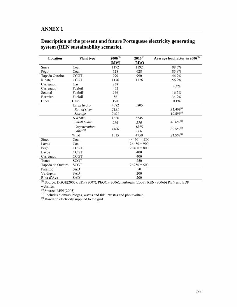
297

ANNEX 1 Description of the present and future Portuguese electricity generating system (REN sustainability scenario).

Location Plant type 2006(1)

(MW)2016(2)

(MW) Average load factor in 2006(1)

Sines Coal 1192 1192 98.3% Pêgo Coal 628 628 85.9% Tapada Outeiro CCGT 990 990 46.9% Ribatejo CCGT 1176 1176 56.9% Carregado Gas 238 4.4% Carregado Fueloil 472 Setubal Fueloil 946 16.2% Barreiro Fueloil 56 34.9% Tunes Gasoil 198 0.1% Large hydro 4582 5805 Run of river 2181 31.4%(4)

Storage 2401 19.5%(4) NWSRP 1626 3245 Small hydro 286 570 40.0%(4) Cogeneration 1400 1875 39.5%(4) Other(3) 800 Wind 1515 4750 21.9%(4) Sines Coal 4×450 = 1800 Lavos Coal 2×450 = 900 Pego CCGT 2×400 = 800 Lavos CCGT 400 Carregado CCGT 400 Tunes SCGT 250 Tapada do Outeiro SCGT 2×250 = 500 Paraimo SAD 50 Valdigem SAD 200 Riba d’Ave SAD 200 (1) Source: DGGE(2007), EDP (2007), PEGOP(2006), Turbogas (2006), REN (2006b) REN and EDP websites. (2) Source: REN (2005). (3) Includes biomass, biogas, waves and tidal, wastes and photovoltaic. (4) Based on electricity supplied to the grid.

298

ANNEX 2 Average fuel consumption, fuel cost and average CO2 emissions. Existing power plants Plant type Fuel consumption

[1] Efficiency

(%) [2] Fuel cost

[3] Fuel cost

(€/MWh) [4] CO2

(ton/MWh) [5] Coal 0.349 ton/MWh 40.2 56.7 €/ton 19.8 0.844 CCGT 174 m3N/MWh 53.5 241 €/103m3N 41.9 0.375 Fueloil 0.223 ton/MWh 40.0 202.6 €/ton 45.2 0.715 SCGT 266 m3N /MWh 35.0 241 €/103m3N 64.1 0.575

[1] Fuel consumption- average unit of fuel consumed (measured in tons of coal and fueloil

and m3N of natural gas) per MWh of electricity produced. Information obtained from

power plants presently operating in the market (EDP, 2006a) and Turbogas (2005).

[2] Average efficiency (%) = 100(MWh)year an in consumed Fuel

(MWh)year an in produced Electricty× , assuming the

following calorific power for each fuel:

Coal - 25584 MJ/ton = 7.11 MWh/ton

Fueloil - 40193 MJ/ton = 11.16 MWh/ton

Natural gas - 42034 MJ/103m3N = 11.68 MWh/103m3N

[3] Fuel cost- average cost per unit of fuel consumed (measured in € per ton for coal and

fueloil and € per m3N of natural gas). Information obtained from power plants presently

operating in the market (EDP, 2006b).

[4] Fuel cost (€/MWh) = [1]×[3]. Average cost per MWh of electricity produced.

[5] CO2 – average CO2 emissions (measured in tons) per MWh of electricity produced.

Information obtained from power plants presently operating in the market (EDP, 2006a)

and Turbogas (2005).

299

Candidate power plants Plant type Efficiency

(%) Fuel consumption Fuel Fuel cost

(€/MWh) CO2

(ton/MWh) SCPC1 46.0 0.305 ton/MWh 56.7 €/ton 17.3 0.738 CCGT2 57.0 163.4 m3N/MWh 241.0 €/103m3N 39.4 0.353 1 Super critical pulverised coal 2 Combined cycle gas turbine Efficiency- Information obtained from IEA/NEA (2005).

The average fuel consumption was calculated from the data for existing power plants. For

simplicity reasons, average values for the efficiency of the power plants were used and it

was assumed that the relationship (%)plant power candidate theof Efficiency

(%)plant power existing theof Efficiency would be

constant regardless of the operating regime.

plantspower existing theofn consumptio Fuel (%)plant power candidate theof Efficiency (%)plant power existing theof Efficiency

plant power candidate theofn consumptio Fuel

×

=

Fuel consumption of candidate coal plants = 349.046

40.2× =0.305 ton/MWh

Fuel consumption of candidate gas plants = 17457

53.55× =163.4 m3N/MWh

CO2 emissions calculated from data for existing power plants, assuming new higher

efficiency values:

CO2 emissions of candidate coal plants = 844.046

40.2× =0.738 ton/MWh

CO2 emissions of candidate gas plants = 375.057

53.55× =0.353 m3N/MWh

300

ANNEX 3

Average load factors Month Hydro Wind Small

hydro (1) Other SRP(3) Fuel oil (4) Run of river (1) Storage (1) Storage (2)

Jan. 48% 34% 14% 32% 54% 33% 23% Feb. 51% 25% 10% 27% 49% 35% 22% Mar. 52% 25% 6% 30% 57% 34% 14% Apr. 48% 16% 3% 26% 49% 35% 6% May 33% 13% 3% 20% 29% 32% 12% Jun. 21% 11% 6% 17% 12% 30% 27% Jul. 14% 14% 6% 19% 6% 34% 32%

Aug. 11% 11% 7% 17% 4% 33% 25% Sep. 17% 11% 6% 16% 4% 35% 47% Oct. 24% 13% 5% 29% 27% 34% 33% Nov. 40% 42% 12% 37% 47% 35% 22% Dec. 52% 55% 16% 46% 57% 38% 24%

Annual 34% 23% 8% 27% 33% 34% 24%Source: REN, 2001- 2006 month data available online. (1) Average regime. (2) Dry regime (non electrical commitments). (3) Cogeneration, biomass, biogas, waves and tidal, wastes and photovoltaic. (4) Barreiro and Carregado (includes natural gas group).

301

ANNEX 4 Computation of the modelled electricity production. Demand forecast Month 2008 2009 2010 2011 2012 2013 2014 2015 2016 2017

Jan. 5533 5759 5995 6241 6536 6844 7167 7506 7860 8231 Feb. 4868 5068 5276 5492 5751 6022 6307 6604 6916 7242 Mar. 5085 5293 5510 5736 6007 6291 6588 6898 7224 7565 Apr. 4268 4443 4625 4814 5042 5279 5529 5790 6063 6349 May 4518 4703 4896 5097 5337 5589 5853 6129 6419 6722 Jun. 4570 4758 4953 5156 5399 5654 5921 6200 6493 6799 Jul. 4962 5166 5377 5598 5862 6139 6428 6732 7049 7382

Aug. 4563 4750 4945 5148 5391 5645 5912 6191 6483 6789 Sep. 4663 4854 5053 5260 5509 5769 6041 6326 6625 6937 Oct. 4738 4933 5135 5345 5598 5862 6138 6428 6732 7049 Nov. 4693 4886 5086 5294 5544 5806 6080 6367 6667 6982 Dec. 5312 5530 5757 5993 6276 6572 6882 7207 7547 7903

Annual (GWh) 57774 60142 62607 65174 68250 71471 74845 78377 82077 85951 Peak load (MW) 9900 10300 10716 11150 11681 12237 12819 13429 14070 14740

Note: The demand forecast was based on REN (2005) yearly projections for electricity consumption and on the monthly pattern of the demand in 2006 obtained from REN website. Installed power (MW) Month 2008 2009 2010 2011 2012 2013 2014 2015 2016 2017

Small hydro 410 427 444 460 482 505 529 555 570 570Other SRP(1) 1789 1929 2079 2209 2302 2398 2499 2604 2675 2675 Run of river 2224 2224 2224 2224 2455 2455 2636 2636 2636 2636

Hydro storage 2358 2358 2358 2358 2496 2958 2958 3166 3166 2358 Fuel oil (2) 766 766 710 0 0 0 0 0 0 0

(1) Cogeneration, biomass, biogas, waves and tidal, wastes and photovoltaic. (2) Barreiro and Carregado (includes natural gas group). Non-modelled production includes:

Production from run of river power plants, including small hydro plants (average

regime).

Production from hydro storage power plants (dry regime).

Production from NWSRP.

Production from fuel oil power plants (Barreiro and Carregado).

These values were computed using data presented in Annex 3.

302

Non modelled production (GWh) Month 2008 2009 2010 2011 2012 2013 2014 2015 2016 2017



Annual 16378 16844 17226 16176 17302 17969 18882 19409 19665 19665 % fuel oil 10% 9% 9% 0% 0% 0% 0% 0% 0% 0%

% small hydro 7% 7% 7% 8% 8% 8% 8% 8% 8% 8% % other SRP (1) 33% 34% 36% 41% 40% 40% 40% 40% 41% 41%

% hydro 50% 49% 48% 51% 52% 52% 52% 52% 51% 51% (1) Cogeneration, biomass, biogas, waves and tidal, wastes and photovoltaic. Modelled demand (GWh) Month 2008 2009 2010 2011 2012 2013 2014 2015 2016 2017


Aug. 3658 3810 3978 4279 4471 4677 4903 5144 5418 5724 Sep. 3576 3732 3912 4327 4518 4734 4959 5208 5488 5801 Oct. 3517 3672 3846 4194 4371 4587 4801 5050 5332 5650Nov. 3135 3286 3451 3734 3875 4064 4252 4486 4763 5078 Dec. 3351 3522 3709 4031 4172 4375 4577 4836 5150 5506

Annual 41385 43288 45371 48988 50938 53485 55948 58951 62395 66269 % Demand 72% 72% 72% 75% 75% 75% 75% 75% 76% 77%

303

ANNEX 5 NWSRP excluding fuel and gas cogeneration (GWh)

Month 2008 2009 2010 2011 2012 2013 2014 2015 2016 2017 Jan. 367 396 427 453 477 502 529 557 574 573 Feb. 333 360 389 414 436 459 483 509 525 525 Mar. 384 414 446 474 499 525 553 582 600 599 Apr. 356 385 416 442 466 490 516 544 560 560 May 290 315 342 366 385 406 428 451 465 465 Jun. 219 240 263 283 298 315 332 350 361 361 Jul. 230 253 279 301 318 335 354 373 385 385


Annual 3681 3997 4341 4633 4884 5148 5424 5713 5893 5891 (1) Assuming that 1/3 of the cogeneration electricity production comes from biomass and 2/3 from fueloil or natural gas combustion.

304

ANNEX 6 Average hydro inflows (GWh)

Month 2008 2009 2010 2011 2012 2013 2014 2015 2016 2017 Jan. 723 723 723 723 765 907 907 971 971 971 Feb. 379 379 379 379 401 476 476 509 509 509 Mar. 592 592 592 592 627 743 743 795 795 795 Apr. 340 340 340 340 360 426 426 456 456 456 May 191 191 191 191 202 240 240 257 257 257 Jun. 66 66 66 66 70 83 83 89 89 89 Jul. 48 48 48 48 51 60 60 64 64 64


Annual 3866 3866 3866 3866 4092 4850 4850 5191 5191 5191

Note: The hydro inflows are based on REN, 2001- 2006 monthly data available online, assuming that these values would increase with the increasing of the hydro storage capacity.

305

ANNEX 7 GAMS code EPM ************************************************************************** ********************* COST OPTIMIZATION **************************** ************************************************************************** * 1a, 1b, 1c coal, 2a, 2b ccgt, 3a wind onshore, 3b wind offshore, 4 coal, 5 ccgt, 6 fueloil, 7 large hydro, * 8 SCGT, 9 wind, 10 offshore" Sets t years /2008*2017 / r(t) renyears /2010*2017/ m months /1*12/ i plants / 1a, 1b, 1c, 2a, 2b, 3a, 3b, 4, 5, 6, 8, 9 / k(i) new plants / 1a, 1b, 1c, 2a, 2b, 3a, 3b/ l(i) existing plants / 4, 5, 6, 8, 9 / h hydro plants /7/ kt(k) new thermal power plants /1a, 1b, 1c, 2a, 2b/ lt(l) non wind existing plants /4, 5, 6, 8/ kw(k) new wind power plants / 3a, 3b/ lw(l) existing wind power power plants /9/ ; Parameters IC(k) investment cost of the new plants (€-MW) / 1a 1137000 1b 1137000 1c 1137000 2a 517000 2b 517000 3a 1213000 3b 1741000/; Parameters FOM(k) fixed OM cost of the new plants (€-MW) / 1a 33800 1b 33800 1c 33800 2a 11300 2b 11300 3a 26600 3b 61300 /; Parameters n(k) life time of the new plants / 1a 35 1b 35 1c 35 2a 24 2b 24 3a 20 3b 20 /; Parameters CP(kt) modular capacity of the new plants (MW) / 1a 300 1b 450

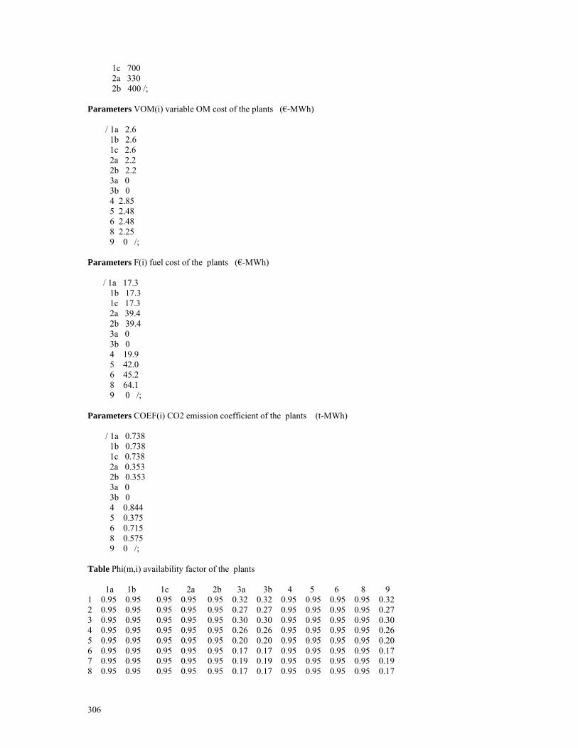
306

1c 700 2a 330 2b 400 /; Parameters VOM(i) variable OM cost of the plants (€-MWh) / 1a 2.6 1b 2.6 1c 2.6 2a 2.2 2b 2.2 3a 0 3b 0 4 2.85 5 2.48 6 2.48 8 2.25 9 0 /; Parameters F(i) fuel cost of the plants (€-MWh) / 1a 17.3 1b 17.3 1c 17.3 2a 39.4 2b 39.4 3a 0 3b 0 4 19.9 5 42.0 6 45.2 8 64.1 9 0 /; Parameters COEF(i) CO2 emission coefficient of the plants (t-MWh) / 1a 0.738 1b 0.738 1c 0.738 2a 0.353 2b 0.353 3a 0 3b 0 4 0.844 5 0.375 6 0.715 8 0.575 9 0 /; Table Phi(m,i) availability factor of the plants 1a 1b 1c 2a 2b 3a 3b 4 5 6 8 9 1 0.95 0.95 0.95 0.95 0.95 0.32 0.32 0.95 0.95 0.95 0.95 0.32 2 0.95 0.95 0.95 0.95 0.95 0.27 0.27 0.95 0.95 0.95 0.95 0.27 3 0.95 0.95 0.95 0.95 0.95 0.30 0.30 0.95 0.95 0.95 0.95 0.30 4 0.95 0.95 0.95 0.95 0.95 0.26 0.26 0.95 0.95 0.95 0.95 0.26 5 0.95 0.95 0.95 0.95 0.95 0.20 0.20 0.95 0.95 0.95 0.95 0.20 6 0.95 0.95 0.95 0.95 0.95 0.17 0.17 0.95 0.95 0.95 0.95 0.17 7 0.95 0.95 0.95 0.95 0.95 0.19 0.19 0.95 0.95 0.95 0.95 0.19 8 0.95 0.95 0.95 0.95 0.95 0.17 0.17 0.95 0.95 0.95 0.95 0.17

307

9 0.95 0.95 0.95 0.95 0.95 0.16 0.16 0.95 0.95 0.95 0.95 0.16 10 0.95 0.95 0.95 0.95 0.95 0.29 0.29 0.95 0.95 0.95 0.95 0.29 11 0.95 0.95 0.95 0.95 0.95 0.37 0.37 0.95 0.95 0.95 0.95 0.37 12 0.95 0.95 0.95 0.95 0.95 0.46 0.46 0.95 0.95 0.95 0.95 0.46 ; Scalar COEFh cO2 emission coefficient for hydro plants /0/; Table IP(t,l) installed power of the existing plants (MW) 4 5 6 8 9 2008 1820 2166 946.4 250 1515 2009 1820 2166 946.4 250 1515 2010 1820 2166 946.4 250 1515 2011 1820 2166 946.4 500 1515 2012 1820 2166 946.4 500 1515 2013 1820 2166 0 500 1515 2014 1820 2166 0 500 1515 2015 1820 2166 0 750 1515 2016 1820 2166 0 750 1515 2017 1820 2166 0 750 1515 ; Parameter year(t) year to index / 2008 1 2009 2 2010 3 2011 4 2012 5 2013 6 2014 7 2015 8 2016 9 2017 10 /; Parameter IPh(t) installed power of the existing hydro plants (MW) / 2008 4582 2009 4582 2010 4582 2011 4582 2012 4951 2013 5413 2014 5597 2015 5805 2016 5805 2017 5805 /; Parameter D(t) demand (MWh) / 2008 57774098 2009 60142258 2010 62607489 2011 65173770 2012 68249972 2013 71471371 2014 74844820 2015 78377495 2016 82076913 2017 85950943 /;

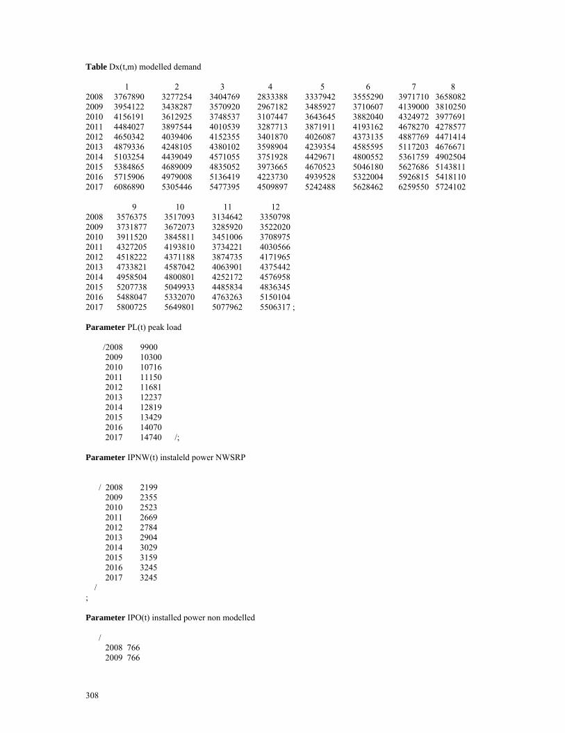
308

Table Dx(t,m) modelled demand 1 2 3 4 5 6 7 8 2008 3767890 3277254 3404769 2833388 3337942 3555290 3971710 3658082 2009 3954122 3438287 3570920 2967182 3485927 3710607 4139000 3810250 2010 4156191 3612925 3748537 3107447 3643645 3882040 4324972 3977691 2011 4484027 3897544 4010539 3287713 3871911 4193162 4678270 4278577 2012 4650342 4039406 4152355 3401870 4026087 4373135 4887769 4471414 2013 4879336 4248105 4380102 3598904 4239354 4585595 5117203 4676671 2014 5103254 4439049 4571055 3751928 4429671 4800552 5361759 4902504 2015 5384865 4689009 4835052 3973665 4670523 5046180 5627686 5143811 2016 5715906 4979008 5136419 4223730 4939528 5322004 5926815 5418110 2017 6086890 5305446 5477395 4509897 5242488 5628462 6259550 5724102

9 10 11 12 2008 3576375 3517093 3134642 3350798 2009 3731877 3672073 3285920 3522020 2010 3911520 3845811 3451006 3708975 2011 4327205 4193810 3734221 4030566 2012 4518222 4371188 3874735 4171965 2013 4733821 4587042 4063901 4375442 2014 4958504 4800801 4252172 4576958 2015 5207738 5049933 4485834 4836345 2016 5488047 5332070 4763263 5150104 2017 5800725 5649801 5077962 5506317 ; Parameter PL(t) peak load /2008 9900 2009 10300 2010 10716 2011 11150 2012 11681 2013 12237 2014 12819 2015 13429 2016 14070 2017 14740 /; Parameter IPNW(t) instaleld power NWSRP / 2008 2199 2009 2355 2010 2523 2011 2669 2012 2784 2013 2904 2014 3029 2015 3159 2016 3245 2017 3245 / ; Parameter IPO(t) installed power non modelled / 2008 766 2009 766

309

2010 710 2011 0 2012 0 2013 0 2014 0 2015 0 2016 0 2017 0 / ; Table PNWx(t,m) NWSRP excluding coal and gas cogeneration (MWh) 1 2 3 4 5 6 7 8 2008 367361 333341 384216 356047 289670 218931 229924 218519 2009 395859 360110 413957 384638 314904 240056 253418 241146 2010 426642 389062 446079 415563 342281 263055 279043 265834 2011 452976 413788 473561 441972 365569 282531 300693 286683 2012 477051 435924 498721 465616 385435 298202 317568 302816 2013 502298 459138 525104 490411 406271 314639 335270 319740 2014 528771 483481 552769 516411 428121 331878 353837 337491 2015 556528 509004 581775 543673 451032 349956 373308 356107 2016 573607 524741 599621 560482 465226 361224 385486 367760 2017 573445 524583 599453 560313 465066 361078 385317 367595

9 10 11 12 2008 222673 298999 351247 409895 2009 245777 325487 379721 442371 2010 270989 354242 410531 477480 2011 292277 378684 436830 507482 2012 308732 399331 460241 534562 2013 325994 420986 484793 562960 2014 344099 443695 510538 592738 2015 363086 467508 537532 623959 2016 374973 482275 554184 643195 2017 374805 482104 554015 643006; Table SH(t,m) Small hydro production (average year) MWh 1 2 3 4 5 6 7 8 9 2008 164212 135268 172730 144491 87724 35261 17246 11887 11394 2009 170945 140814 179812 150415 91321 36707 17953 12374 11862 2010 177954 146588 187184 156582 95065 38212 18689 12882 12348 2011 184238 151764 193795 162112 98422 39561 19349 13336 12784 2012 193082 159049 203097 169893 103147 41460 20277 13977 13398 2013 202349 166683 212845 178048 108098 43451 21251 14647 14041 2014 212062 174684 223062 186594 113286 45536 22271 15351 14715 2015 222241 183069 233769 195551 118724 47722 23340 16087 15421 2016 228295 188056 240137 200877 121958 49022 23976 16526 15841 2017 228295 188056 240137 200877 121958 49022 23976 16526 15841

10 11 12 2008 83874 138472 172973 2009 87313 144149 180065 2010 90893 150059 187447 2011 94103 155359 194067 2012 98620 162816 203382 2013 103353 170631 213144 2014 108314 178821 223375 2015 113513 187405 234097

310

2016 116606 192510 240474 2017 116606 192510 240474 ; Table PNMH(t,m) hydro power production non modelled (MWh) 1 2 3 4 5 6 7 8 2008 1037596 920517 974720 806995 594309 438931 339659 311388 2009 1037596 920517 974720 806995 594309 438931 339659 311388 2010 1037596 920517 974720 806995 594309 438931 339659 311388 2011 1037596 920517 974720 806995 594309 438931 339659 311388 2012 1134538 1008660 1070951 888877 653628 480078 369905 338018 2013 1181336 1040931 1092601 897251 664044 499279 391653 362705 2014 1246342 1102442 1162936 959450 708085 527026 410263 377793 2015 1267411 1116971 1172683 963220 712775 535670 420054 388907 2016 1267411 1116971 1172683 963220 712775 535670 420054 388907 2017 1267411 1116971 1172683 963220 712775 535670 420054 388907

9 10 11 12 2008 363546 490499 844018 1143739 2009 363546 490499 844018 1143739 2010 363546 490499 844018 1143739 2011 363546 490499 844018 1143739 2012 396818 537092 922389 1249659 2013 416214 555902 962554 1305302 2014 437745 588008 1014560 1375272 2015 446477 596476 1032644 1400324 2016 446477 596476 1032644 1400324 2017 446477 596476 1032644 1400324 ; Table afl(t,m) modelled storage (MWh) 1 2 3 4 5 6 7 8 2008 1921313 214461 481668 296927 138002 -32000 -63000 -85167 2009 484313 214461 481668 296927 138002 -32000 -63000 -85167 2010 484313 214461 481668 296927 138002 -32000 -63000 -85167 2011 484313 214461 481668 296927 138002 -32000 -63000 -85167 2012 512657 227012 509857 314304 146079 -33873 -66687 -90151 2013 607548 269031 604230 372480 173117 -40142 -79031 -106838 2014 607548 269031 604230 372480 173117 -40142 -79031 -106838 2015 650269 287949 646718 398672 185290 -42965 -84588 -114350 2016 650269 287949 646718 398672 185290 -42965 -84588 -114350 2017 650269 287949 646718 398672 185290 -42965 -84588 -114350

9 10 11 12 2008 -53000 313167 292833 248667 2009 -53000 313167 292833 248667 2010 -53000 313167 292833 248667 2011 -53000 313167 292833 248667 2012 -561002 331494 309971 263220 2013 -66486 392853 367346 311941 2014 -66486 392853 367346 311941 2015 -71161 420477 393177 333876 2016 -71161 420477 393177 333876 2017 -71161 420477 393177 -1103124 *Notes: *January 2008 includes 1437 GWh from initial reserve.

311

*December 2017 subtracts 1437 to ensure that final reserve = intial reserve *negative values in months with low water inflows. Means that hydro production * in that months is restricted to the non modelled or comes from * the water accumulated from previous months ; Parameter delta(m) hours of the month / 1 744 2 672 3 744 4 720 5 744 6 720 7 744 8 744 9 720 10 744 11 720 12 744 /; Scalar j interest rate /0.05/ ; Scalar EC esmission cost /22/ ; Scalar LTG loss thermal group /392/ ; Scalar LHG loss hydro group/315/ ; Scalar Q3 non-available capacity wind/0.73/ ; Scalar Q7 non-available capacity hydro/0.3/ ; Scalar QNW non-available capacity NWSRP/0.5/ ; Scalar RM reference margin/0.052/ ; Variables IPN(t,k) installed power P(t,m,i) power output theta(t,kt) modular thermal power ph(t,m) hydro power output tc total cost co cO2 emissions Res(t,m) reserve ; Positive variable IPN; Positive variable P; positive variable Ph; integer variable theta; Positive variable res; IPN.up(t,k)=10000; P.up(t,m,i)=10000; theta.up(t,kt)=25; ph.up(t,m)=2000; Equations totalCO define objective function totalcost define objective function demand(t,m) observe demand capacity(t,kt) modular capacity

312

reference(t) observe RM powerk(t,m,kt) observe power limits for new plants powerl(t,m,lt) observe power limits for existing plants ren(r) observe renewable limits windk(t,m,kw) observe wind priority windl (t,m,lw) observe wind priority windon(t,kw) observe wind onshore potential windoff(t,kw) observe wind offshore potential reference2(t) avoid unecessary capacity when minimizing emissions COconstraint observe CO limits acumulated(t,k) observe increasing IPN reserve(t,m) reserve reserve1(t) reserve in Jan reserve2(t) reserve in Feb reserve3(t) reserve in Mar reserve4(t) reserve in Apr reserve5(t) reserve in May reserve6(t) reserve in Jun reserve7(t) reserve in Jul reserve8(t) reserve in Aug reserve9(t) reserve in Sept reserve10(t) reserve in Oct reserve11(t) reserve in Nov reserve12(t) reserve in Dec minRes(t,m) minimum reserve maxRes(t,m) maximum reserve GNminimum(t,m) flexibility to the system ; totalCO.. co=e=sum((t,m,i),COEF(i)*P(t,m,i)*delta(m))+sum((t,m),COEFh*Ph(t,m)*delta(m)); totalcost.. tc=e=(sum((t,k),(j*power((1+j),n(k))/(power((1+j),n(k))-1)*IC(k)+FOM(k))*IPN(t,k)*power((1+j),-year(t))) +sum((t,m,i),(VOM(i)+F(i)+COEF(i)*EC)*P(t,m,i)*delta(m)*power((1+j),-year(t))))/1000; demand(t,m).. sum(i,P(t,m,i))+PH(t,m)=g=Dx(t,m)/delta(m); powerk(t,m,kt).. P(t,m,kt)=l=IPN(t,kt)*phi(m,kt); powerl(t,m,lt).. P(t,m,lt)=l=IP(t,lt)*phi(m,lt); reserve1(t).. res(t,'1')=e=res(t-1,'12')+afl(t,'1')-Ph(t,'1')*delta('1'); reserve2(t).. res(t,'2')=e=res(t,'1')+afl(t,'2')-Ph(t,'2')*delta('2'); reserve3(t).. res(t,'3')=e=res(t,'2')+afl(t,'3')-Ph(t,'3')*delta('3'); reserve4(t).. res(t,'4')=e=res(t,'3')+afl(t,'4')-Ph(t,'4')*delta('4'); reserve5(t).. res(t,'5')=e=res(t,'4')+afl(t,'5')-Ph(t,'5')*delta('5'); reserve6(t).. res(t,'6')=e=res(t,'5')+afl(t,'6')-Ph(t,'6')*delta('6'); reserve7(t).. res(t,'7')=e=res(t,'6')+afl(t,'7')-Ph(t,'7')*delta('7'); reserve8(t).. res(t,'8')=e=res(t,'7')+afl(t,'8')-Ph(t,'8')*delta('8'); reserve9(t).. res(t,'9')=e=res(t,'8')+afl(t,'9')-Ph(t,'9')*delta('9'); reserve10(t).. res(t,'10')=e=res(t,'9')+afl(t,'10')-Ph(t,'10')*delta('10'); reserve11(t).. res(t,'11')=e=res(t,'10')+afl(t,'11')-Ph(t,'11')*delta('11'); reserve12(t).. res(t,'12')=e=res(t,'11')+afl(t,'12')-Ph(t,'12')*delta('12'); minRes(t,m).. res(t,m)=g=1200000; maxRes(t,m).. res(t,m)=l=3000000; capacity(t,kt).. IPN(t,kt)=e=theta(t,kt)*CP(kt);

313

reference(t).. sum(l,IP(t,l))+sum(k,IPN(t,k))+IPh(t)+IPNW(t)+IPO(t)- (Q3*(IPN(t,'3a')+IPN(t,'3b')+IP(t,'9'))+Q7*IPh(t) +QNW*IPNW(t)+LTG+LHG)-PL(t)-RM*(sum(l,IP(t,l))+sum(k,IPN(t,k))+IPh(t)+IPNW(t)+IPO(t))=g=0; reference2(t).. sum(l,IP(t,l))+sum(k,IPN(t,k))+IPh(t)+IPNW(t)+IPO(t)-(Q3*(IPN(t,'3a')+IPN(t,'3b')+IP(t,'9')) +Q7*IPh(t)+QNW*IPNW(t)+LTG+LHG)-PL(t)-(RM+.2)*(sum(l,IP(t,l))+sum(k,IPN(t,k))+IPh(t)+IPNW(t)+IPO(t))=l=0; ren(r).. sum(m,((P(r,m,'3a')+P(r,m,'3b')+P(r,m,'9')+Ph(r,m)*1.22)*delta(m)))+sum(m,Pnmh(r,m)*1.22) +sum(m,PNWx(r,m)-SH(r,m)+SH(r,m)*1.22)=g=0.39*D(r); windk(t,m,kw).. P(t,m,kw)=e=IPN(t,kw)*phi(m,kw); windl(t,m,lw).. P(t,m,lw)=e=IP(t,lw)*phi(m,lw); windon(t,kw).. IPN(t,'3a')=l=6500; windoff(t,kw).. IPN(t,'3b')=l=1000; acumulated(t,k).. IPN(t,k)=g=IPN(t-1,k); COconstraint.. sum((t,m,i),COEF(i)*P(t,m,i)*delta(m))+sum((t,m),COEFh*Ph(t,m)*delta(m))=l=2.0e8; GNminimum(t,m).. P(t,m,'2a')+P(t,m,'2b')+P(t,m,'5')=g=310; Model windtotal / totalcost, demand, capacity, powerk, powerl, reference, windk, windl, windon, windoff, acumulated, totalco, reserve1,reserve2, reserve3, reserve4, reserve5, reserve6, reserve7, reserve8, reserve9, reserve10, reserve11, reserve12, minRes, maxRes, ren, gnminimum/; option optcr = 0.0 ; OPTION RESLIM = 5000000; windtotal.iterlim =10000000; option minlp=baron; Solve windtotal minimizing tc using minlp; parameter IPcoal(t); parameter IPgas(t); parameter IPwind(t); IPcoal(t)=IPN.l(t,'1a')+IPN.l(t,'1b')+IPN.l(t,'1c'); IPgas(t)=IPN.l(t,'2a')+IPN.l(t,'2b'); IPwind(t)=IPN.l(t,'3a')+IPN.l(t,'3b'); parameter PcoalNew total production of coal new; parameter PcoalOld total production of coal old; parameter PgasNew total production of gas new; parameter PgasOld total production of gas old; parameter Pwind total production of wind; PcoalNew= sum((m),(P.l('2017',m,'1a')+P.l('2017',m,'1b')+P.l('2017',m,'1c'))*delta(m)); PgasNew= sum((m),(P.l('2017',m,'2a')+P.l('2017',m,'2b'))*delta(m)); PcoalOld= sum((m),P.l('2017',m,'4')*delta(m)); PgasOld= sum((m),P.l('2017',m,'5')*delta(m));

314

Pwind= sum((m),(P.l('2017',m,'3a')+P.l('2017',m,'3b')+P.l('2017',m,'9'))*delta(m)); parameter H2017 total hydro production; H2017=sum((m),ph.l('2017',m)*delta(m)); parameter P2017 total production in 2017; P2017=PcoalNew+PgasNew+Pcoalold+PgasOld+Pwind+H2017; Parameter VarCost 2017 variable production cost; VarCost= sum((m,i),(VOM(i)+F(i)+COEF(i)*EC)*P.l('2017',m,i)*delta(m)) ; parameter CostP(i) variable cost of plant i; CostP(i)= VOM(i)+F(i)+COEF(i)*EC; Parameter AvVar2017 variable production cost 2017; AvVar2017=VarCost/sum((m),Dx('2017',m)); parameter AnnualCost(t) annual cost; AnnualCost(t)= (sum((k),(j*power((1+j),n(k))/(power((1+j),n(k))-1)*IC(k)+FOM(k))*IPN.l(t,k)*power((1+j),-year(t)))+ sum((m,i),(VOM(i)+F(i)+COEF(i)*EC)*P.l(t,m,i)*power((1+j),-year(t))*delta(m)))/1000 ; parameter AnnualCO(t) annual CO2; AnnualCO(t)= sum((m,i),COEF(i)*P.l(t,m,i)*delta(m)+COEFh*Ph.l(t,m)*delta(m)); parameter AVcost average cost; AVcost=(sum((t,k),(j*power((1+j),n(k))/(power((1+j),n(k))-1)*IC(k)+FOM(k))*IPN.l(t,k)*power((1+j),-year(t))) +sum((t,m,i),(VOM(i)+F(i)+COEF(i)*EC)*P.l(t,m,i)*delta(m)*power((1+j),-year(t))))/sum((t,m),Dx(t,m)); parameter AVCO average emissions; AVCO=(sum((t,m,i),COEF(i)*P.l(t,m,i)*delta(m))+sum((t,m),COEFh*Ph.l(t,m)*delta(m)))/sum((t,m),Dx(t,m)); display AVcost, AVCO; display AnnualCost, AnnualCO; display AvVar2017; display PcoalNew, PgasNew, Pcoalold, PgasOld, Pwind, H2017, P2017; display IPcoal, IPgas, IPwind;

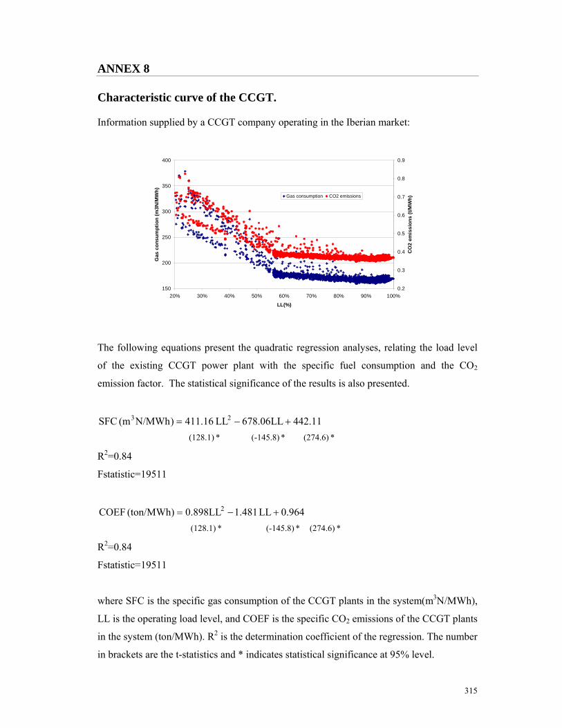
315

ANNEX 8 Characteristic curve of the CCGT. Information supplied by a CCGT company operating in the Iberian market:

150

200

250

300

350

400

20% 30% 40% 50% 60% 70% 80% 90% 100%

LL(%)

Gas

con

sum

ptio

n (m

3N/M

Wh)

0.2

0.3

0.4

0.5

0.6

0.7

0.8

0.9

CO

2 em

issi

ons

(t/M

Wh)Gas consumption CO2 emissions

The following equations present the quadratic regression analyses, relating the load level

of the existing CCGT power plant with the specific fuel consumption and the CO2

emission factor. The statistical significance of the results is also presented.

*(274.6) *(-145.8) *(128.1) 1 1.442LL06.678LL 16.411)N/MWh(m SFC 23 +−=

R2=0.84

Fstatistic=19511

*(274.6) *(-145.8) *(128.1) 964.0LL 481.1LL898.0(ton/MWh) COEF 2 +−=

R2=0.84

Fstatistic=19511

where SFC is the specific gas consumption of the CCGT plants in the system(m3N/MWh),

LL is the operating load level, and COEF is the specific CO2 emissions of the CCGT plants

in the system (ton/MWh). R2 is the determination coefficient of the regression. The number

in brackets are the t-statistics and * indicates statistical significance at 95% level.

316

For the new CCGT it was assumed that the shape of the relationship would be the same,

but the expected higher efficiency leads to new functions. According to Tables 5.1 and 5.4,

the average efficiency of new CCGT is expected to be 57% and the average efficiency of

existing CCGT is 54%. For simplicity reasons, it was assumed that the 0.54/0.57

relationship would hold regardless of the output or load level of the power plants. The

following equations describe the assumed relationships for the new CCGT:

35.415LL02.637LL 28.386)N/MWh(m SFC 23 +−=

907.0LL 391.1LL843.0(ton/MWh) COEF 2 +−=

317

ANNEX 9 CCGT load distribution Annex 9.1 Quadratic CCGT characteristic curves

According to Section V.6.2, the NLEPM assumes a theoretical distribution of the load for

the CCGT system during each interval of the planning period:

• each CCGT subsystems will be operating at average load levels

(characterised by equations 5.31-5.34) for producing 50% of their electricity

supply;

• each CCGT subsystems will be operating at a load level 10% higher than

the average for producing 25% of their electricity supply;

• each CCGT subsystems will be operating at a load level 10% lower than the

average for producing 25% of their electricity supply;

As an example, if the installed wind power is equal to 8000 MW in year t, from equation

5.30 the average load level of the CCGT system the model is equal to:

50.0914.0800010178.5LL -5CCGT =+××−= :

Thus:

• each CCGT subsystems will be operating at average load levels equal to

50% for producing 50% of their electricity supply in each month of year t;

• each CCGT subsystems will be operating at a load level equal to 40% to

produce 25% of their electricity supply in each month of year t;

• each each CCGT subsystems will be operating at a load level equal to 60%

to produce the remaining 25% of their electricity supply in each month of

year t.

And, from equations 5.37, 5.41 and 5.45 the SFC of the existing CCGT subsystem may be

computed for the assumed distribution in year t:

318

25% ( ) ( ) /MWh m 236.9 162.60008 10 4.668000101.10 SFC 3-42-6a5t =+××+×=

50% ( ) ( ) /MWh m 0.062165.88000 103.798000 101.10 SFC 3-32-6

b5t =+××−×= 25% ( ) ( ) /MWh m 187.3177.38000 108.058000 101.10 SFC 3-32-6

c5t =+××−×=

Assuming that the electricity production from CCGT in a certain month of year t is equal to

1000 GWh, the total gas consumption would be:

1000000) (0.25187.31000000) (0.50206.01000000) (0.25236.9n consumptio Gas ××+××+××=

Gas consumption = 210.1×106 m3

If no load distribution was taken into account and only average functions were used to

characterise each CCGT subsystem, the model would be implicitly assuming that all

CCGT were operating at the same load level and the total gas consumption for this

example would be:

Gas consumption = 1000000 0.062 ×


This simple example demonstrates the need to know the load distribution across the CCGT

system or at least to assume a theoretical distribution of the load in order that the model

reflects a more realistic situation.

Annex 9.2 Linear CCGT characteristic curves

Even if the characteristic curves of the CCGT subsystems were considered linear, the need

to assume a theoretical distribution of the load would remain. Assuming that the SFC of the

existing CCGT subsystem could be obtained from:

25% ( ) ( ) 8.171IPIPIP 1014.2 SFC t3b,t3a,9t3

a5t +++×= − 50% ( ) ( ) 7.167IPIPIP 1014.2 SFC t3b,t3a,9t

3b5t +++×= −

319

25% ( ) ( ) 5.163IPIPIP 1014.2 SFC t3b,t3a,9t3

c5t +++×= − For the previous example with total installed wind power equal to 8000 MW and total

electricity production from CCGT in a certain month of year t is equal to 1000 GWh, the

total fuel consumption would be:

25% ( ) 8.1718000 1014.2 SFC 3

a5t +××= − =188.9 m3/MWh

50% ( ) 7.1678000 1014.2 SFC 3

b5t +××= − =195.5 m3/MWh 25% ( ) 5.1638000 1014.2 SFC 3

c5t +××= − =191.3 m3/MWh

1000000) 0.25( 191.31000000) 0.50(195.51000000) 0.25(188.9n consumptio Gas ××+××+××= Gas consumption = 192.8×106 m3

If no load distribution was taken into account and only average functions were used to

characterise each CCGT subsystem, the total gas consumption for this example would be:

Gas consumption = 1000000 195.5×


Demonstrating once more the need to know or assume a theoretical load distribution across

the CCGT system

320

ANNEX 10 GAMS code NLEPM ************************************************************************** ********************* COST OPTIMIZATION **************************** ************************************************************************** * 1a, 1b, 1c coal, 2a, 2b ccgt, 3a wind onshore, 3b wind offshore, 4 coal, 5 ccgt, 6 fueloil, 7 large hydro, * 8 SCGT, 9 wind, 10 offshore" Sets t years /2008*2017 / r(t) renyears /2010*2017/ m months /1*12/ i plants / 1a, 1b, 1c, 2a, 2b, 3a, 3b, 4, 5, 6, 8, 9 / k(i) new plants / 1a, 1b, 1c, 2a, 2b, 3a, 3b/ l(i) existing plants / 4, 5, 6, 8, 9 / h hydro plants /7/ kt(k) new thermal power plants /1a, 1b, 1c, 2a, 2b/ lt(l) non wind existing plants /4, 5, 6, 8/ kw(k) new wind power plants / 3a, 3b/ lw(l) existing wind power power plants /9/ ; Parameters IC(k) investment cost of the new plants (€-MW) / 1a 1137000 1b 1137000 1c 1137000 2a 517000 2b 517000 3a 1213000 3b 1741000/; Parameters FOM(k) fixed OM cost of the new plants (€-MW) / 1a 33800 1b 33800 1c 33800 2a 11300 2b 11300 3a 26600 3b 61300 /; Parameters n(k) life time of the new plants / 1a 35 1b 35 1c 35 2a 24 2b 24 3a 20 3b 20 /; Parameters CP(kt) modular capacity of the new plants (MW) / 1a 300 1b 450

321

1c 700 2a 330 2b 400 /; Parameters VOM(i) variable OM cost of the plants (€-MWh) / 1a 2.6 1b 2.6 1c 2.6 2a 2.2 2b 2.2 3a 0 3b 0 4 2.85 5 2.48 6 2.48 8 2.25 9 0 /; Parameters F(i) fuel cost of the plants (€-MWh) / 1a 17.3 1b 17.3 1c 17.3 2a 0 2b 0 3a 0 3b 0 4 19.9 5 0 6 45.2 8 64.1 9 0 /; Parameters COEF(i) CO2 emission coefficient of the plants (t-MWh) / 1a 0.738 1b 0.738 1c 0.738 2a 0 2b 0 3a 0 3b 0 4 0.844 5 0 6 0.715 8 0.575 9 0 /; Table Phi(m,i) availability factor of the plants 1a 1b 1c 2a 2b 3a 3b 4 5 6 8 9 1 0.95 0.95 0.95 0.95 0.95 0.32 0.32 0.95 0.95 0.95 0.95 0.32 2 0.95 0.95 0.95 0.95 0.95 0.27 0.27 0.95 0.95 0.95 0.95 0.27 3 0.95 0.95 0.95 0.95 0.95 0.30 0.30 0.95 0.95 0.95 0.95 0.30 4 0.95 0.95 0.95 0.95 0.95 0.26 0.26 0.95 0.95 0.95 0.95 0.26 5 0.95 0.95 0.95 0.95 0.95 0.20 0.20 0.95 0.95 0.95 0.95 0.20 6 0.95 0.95 0.95 0.95 0.95 0.17 0.17 0.95 0.95 0.95 0.95 0.17 7 0.95 0.95 0.95 0.95 0.95 0.19 0.19 0.95 0.95 0.95 0.95 0.19 8 0.95 0.95 0.95 0.95 0.95 0.17 0.17 0.95 0.95 0.95 0.95 0.17

322

9 0.95 0.95 0.95 0.95 0.95 0.16 0.16 0.95 0.95 0.95 0.95 0.16 10 0.95 0.95 0.95 0.95 0.95 0.29 0.29 0.95 0.95 0.95 0.95 0.29 11 0.95 0.95 0.95 0.95 0.95 0.37 0.37 0.95 0.95 0.95 0.95 0.37 12 0.95 0.95 0.95 0.95 0.95 0.46 0.46 0.95 0.95 0.95 0.95 0.46 ; Scalar COEFh cO2 emission coefficient for hydro plants /0/; Table IP(t,l) installed power of the existing plants (MW) 4 5 6 8 9 2008 1820 2166 946.4 250 1515 2009 1820 2166 946.4 250 1515 2010 1820 2166 946.4 250 1515 2011 1820 2166 946.4 500 1515 2012 1820 2166 946.4 500 1515 2013 1820 2166 0 500 1515 2014 1820 2166 0 500 1515 2015 1820 2166 0 750 1515 2016 1820 2166 0 750 1515 2017 1820 2166 0 750 1515 ; Parameter year(t) year to index / 2008 1 2009 2 2010 3 2011 4 2012 5 2013 6 2014 7 2015 8 2016 9 2017 10 /; Parameter IPh(t) installed power of the existing hydro plants (MW) / 2008 4582 2009 4582 2010 4582 2011 4582 2012 4951 2013 5413 2014 5597 2015 5805 2016 5805 2017 5805 /; Parameter D(t) demand (MWh) / 2008 57774098 2009 60142258 2010 62607489 2011 65173770 2012 68249972 2013 71471371 2014 74844820 2015 78377495 2016 82076913 2017 85950943 /;

323

Table Dx(t,m) modelled demand 1 2 3 4 5 6 7 8 2008 3767890 3277254 3404769 2833388 3337942 3555290 3971710 3658082 2009 3954122 3438287 3570920 2967182 3485927 3710607 4139000 3810250 2010 4156191 3612925 3748537 3107447 3643645 3882040 4324972 3977691 2011 4484027 3897544 4010539 3287713 3871911 4193162 4678270 4278577 2012 4650342 4039406 4152355 3401870 4026087 4373135 4887769 4471414 2013 4879336 4248105 4380102 3598904 4239354 4585595 5117203 4676671 2014 5103254 4439049 4571055 3751928 4429671 4800552 5361759 4902504 2015 5384865 4689009 4835052 3973665 4670523 5046180 5627686 5143811 2016 5715906 4979008 5136419 4223730 4939528 5322004 5926815 5418110 2017 6086890 5305446 5477395 4509897 5242488 5628462 6259550 5724102

9 10 11 12 2008 3576375 3517093 3134642 3350798 2009 3731877 3672073 3285920 3522020 2010 3911520 3845811 3451006 3708975 2011 4327205 4193810 3734221 4030566 2012 4518222 4371188 3874735 4171965 2013 4733821 4587042 4063901 4375442 2014 4958504 4800801 4252172 4576958 2015 5207738 5049933 4485834 4836345 2016 5488047 5332070 4763263 5150104 2017 5800725 5649801 5077962 5506317 ; Parameter PL(t) peak load /2008 9900 2009 10300 2010 10716 2011 11150 2012 11681 2013 12237 2014 12819 2015 13429 2016 14070 2017 14740 /; Parameter IPNW(t) instaleld power NWSRP / 2008 2199 2009 2355 2010 2523 2011 2669 2012 2784 2013 2904 2014 3029 2015 3159 2016 3245 2017 3245 / ; Parameter IPO(t) installed power non modelled / 2008 766 2009 766 2010 710

324

2011 0 2012 0 2013 0 2014 0 2015 0 2016 0 2017 0 / ; Table PNWx(t,m) NWSRP excluding coal and gas cogeneration (MWh) 1 2 3 4 5 6 7 8 2008 367361 333341 384216 356047 289670 218931 229924 218519 2009 395859 360110 413957 384638 314904 240056 253418 241146 2010 426642 389062 446079 415563 342281 263055 279043 265834 2011 452976 413788 473561 441972 365569 282531 300693 286683 2012 477051 435924 498721 465616 385435 298202 317568 302816 2013 502298 459138 525104 490411 406271 314639 335270 319740 2014 528771 483481 552769 516411 428121 331878 353837 337491 2015 556528 509004 581775 543673 451032 349956 373308 356107 2016 573607 524741 599621 560482 465226 361224 385486 367760 2017 573445 524583 599453 560313 465066 361078 385317 367595

9 10 11 12 2008 222673 298999 351247 409895 2009 245777 325487 379721 442371 2010 270989 354242 410531 477480 2011 292277 378684 436830 507482 2012 308732 399331 460241 534562 2013 325994 420986 484793 562960 2014 344099 443695 510538 592738 2015 363086 467508 537532 623959 2016 374973 482275 554184 643195 2017 374805 482104 554015 643006; Table SH(t,m) Small hydro production (average year) MWh 1 2 3 4 5 6 7 8 9 2008 164212 135268 172730 144491 87724 35261 17246 11887 11394 2009 170945 140814 179812 150415 91321 36707 17953 12374 11862 2010 177954 146588 187184 156582 95065 38212 18689 12882 12348 2011 184238 151764 193795 162112 98422 39561 19349 13336 12784 2012 193082 159049 203097 169893 103147 41460 20277 13977 13398 2013 202349 166683 212845 178048 108098 43451 21251 14647 14041 2014 212062 174684 223062 186594 113286 45536 22271 15351 14715 2015 222241 183069 233769 195551 118724 47722 23340 16087 15421 2016 228295 188056 240137 200877 121958 49022 23976 16526 15841 2017 228295 188056 240137 200877 121958 49022 23976 16526 15841

10 11 12 2008 83874 138472 172973 2009 87313 144149 180065 2010 90893 150059 187447 2011 94103 155359 194067 2012 98620 162816 203382 2013 103353 170631 213144 2014 108314 178821 223375 2015 113513 187405 234097 2016 116606 192510 240474

325

2017 116606 192510 240474 ; Table PNMH(t,m) hydro power production non modelled (MWh) 1 2 3 4 5 6 7 8 2008 1037596 920517 974720 806995 594309 438931 339659 311388 2009 1037596 920517 974720 806995 594309 438931 339659 311388 2010 1037596 920517 974720 806995 594309 438931 339659 311388 2011 1037596 920517 974720 806995 594309 438931 339659 311388 2012 1134538 1008660 1070951 888877 653628 480078 369905 338018 2013 1181336 1040931 1092601 897251 664044 499279 391653 362705 2014 1246342 1102442 1162936 959450 708085 527026 410263 377793 2015 1267411 1116971 1172683 963220 712775 535670 420054 388907 2016 1267411 1116971 1172683 963220 712775 535670 420054 388907 2017 1267411 1116971 1172683 963220 712775 535670 420054 388907

9 10 11 12 2008 363546 490499 844018 1143739 2009 363546 490499 844018 1143739 2010 363546 490499 844018 1143739 2011 363546 490499 844018 1143739 2012 396818 537092 922389 1249659 2013 416214 555902 962554 1305302 2014 437745 588008 1014560 1375272 2015 446477 596476 1032644 1400324 2016 446477 596476 1032644 1400324 2017 446477 596476 1032644 1400324 ; Table afl(t,m) modelled storage (MWh) 1 2 3 4 5 6 7 8 2008 1921313 214461 481668 296927 138002 -32000 -63000 -85167 2009 484313 214461 481668 296927 138002 -32000 -63000 -85167 2010 484313 214461 481668 296927 138002 -32000 -63000 -85167 2011 484313 214461 481668 296927 138002 -32000 -63000 -85167 2012 512657 227012 509857 314304 146079 -33873 -66687 -90151 2013 607548 269031 604230 372480 173117 -40142 -79031 -106838 2014 607548 269031 604230 372480 173117 -40142 -79031 -106838 2015 650269 287949 646718 398672 185290 -42965 -84588 -114350 2016 650269 287949 646718 398672 185290 -42965 -84588 -114350 2017 650269 287949 646718 398672 185290 -42965 -84588 -114350

9 10 11 12 2008 -53000 313167 292833 248667 2009 -53000 313167 292833 248667 2010 -53000 313167 292833 248667 2011 -53000 313167 292833 248667 2012 -561002 331494 309971 263220 2013 -66486 392853 367346 311941 2014 -66486 392853 367346 311941 2015 -71161 420477 393177 333876 2016 -71161 420477 393177 333876 2017 -71161 420477 393177 -1103124 *Notes: *January 2008 includes 1437 GWh from initial reserve. *December 2017 subtracts 1437 to ensure that final reserve = intial reserve *negative values in months with low water inflows. Means that hydro production

326

* in that months is restricted to the non modelled or comes from * the water accumulatedfrom previous months ; Parameter delta(m) hours of the month / 1 744 2 672 3 744 4 720 5 744 6 720 7 744 8 744 9 720 10 744 11 720 12 744 /; Scalar j interest rate /0.05/ ; Scalar EC esmission cost /22/ ; Scalar LTG loss thermal group /392/ ; Scalar LHG loss hydro group/315/ ; Scalar Q3 non-available capacity wind/0.73/ ; Scalar Q7 non-available capacity hydro/0.3/ ; Scalar QNW non-available capacity NWSRP/0.5/ ; Scalar RM reference margin/0.052/ ; Variables IPN(t,k) installed power P(t,m,i) power output theta(t,kt) modular thermal power ph(t,m) hydro power output tc total cost co cO2 emissions Res(t,m) reserve GN(t) gas consumption new CCGT plants GO(t) gas consumption old CCGT plants G1(t) auxiliar variable for gas consumption G2(t) auxiliar variable for gas consumption G3(t) auxiliar variable for gas consumption G4(t) auxiliar variable for gas consumption CON(t) COEF new power plants COO(t) COEF old power plants ; Positive variable IPN; Positive variable P; positive variable Ph; integer variable theta; Positive variable res; Positive variable gn; Positive variable go; Positive variable COn; Positive variable COo; IPN.up(t,k)=10000; P.up(t,m,i)=10000; theta.up(t,kt)=25;

327

ph.up(t,m)=2000; GN.up(t)=500; GO.up(t)=500; CON.up(t)=1; COO.up(t)=1; Equations totalCO define objective function totalcost define objective function demand(t,m) observe demand capacity(t,kt) modular capacity reference(t) observe RM powerk(t,m,kt) observe power limits for new plants powerl(t,m,lt) observe power limits for existing plants ren(r) observe renewable limits windk(t,m,kw) observe wind priority windl (t,m,lw) observe wind priority windon(t,kw) observe wind onshore potential windoff(t,kw) observe wind offshore potential reference2(t) avoid unecessary capacity when minimizing emissions COconstraint observe CO limits acumulated(t,k) observe increasing IPN reserve(t,m) reserve reserve1(t) reserve in Jan reserve2(t) reserve in Feb reserve3(t) reserve in Mar reserve4(t) reserve in Apr reserve5(t) reserve in May reserve6(t) reserve in Jun reserve7(t) reserve in Jul reserve8(t) reserve in Aug reserve9(t) reserve in Sep reserve10(t) reserve in Oct reserve11(t) reserve in Nov reserve12(t) reserve in Dec minRes(t,m) minimum reserve maxRes(t,m) maximum reserve Gasnew1(t) gas consumption new CCGT Gasold1(t) gas consumption old CCGT COnew1(t) CO2 new CCGT COold1(t) CO2 old CCGT GNminimum(t,m) flexibility to the system ; totalCO.. co=e=(sum((t,m,i),COEF(i)*P(t,m,i)*delta(m))+sum((t,m),COEFh*Ph(t,m)*delta(m)) + sum((t,m),CON(t)*(P(t,m,'2a')+P(t,m,'2b'))*delta(m)) + sum((t,m),COO(t)*P(t,m,'5')*delta(m)))/1000; totalcost.. tc=e=(sum((t,k),(j*power((1+j),n(k))/(power((1+j),n(k))-1)*IC(k)+FOM(k))*IPN(t,k)*power((1+j),-year(t))) +sum((t,m,i),(VOM(i)+F(i)+COEF(i)*EC)*P(t,m,i)*delta(m)*power((1+j),-year(t))) + sum((t,m),gn(t)*(P(t,m,'2a')+P(t,m,'2b'))*delta(m)*power((1+j),-year(t)))*241e-3 +sum((t,m),go(t)*P(t,m,'5')*delta(m)*power((1+j),-year(t)))*241e-3

328

+ sum((t,m),CON(t)*(P(t,m,'2a')+P(t,m,'2b'))*delta(m)*power((1+j),-year(t)))*EC +sum((t,m),COO(t)*P(t,m,'5')*delta(m)*power((1+j),-year(t)))*EC)/1000000 ; gasold1(t).. go(t)=e=(1.102e-6*(IPN(t,'3a')+IPN(t,'3b')+IP(t,'9'))*(IPN(t,'3a')+IPN(t,'3b')+IP(t,'9'))- 3.792e-3*(IPN(t,'3a')+IPN(t,'3b')+IP(t,'9'))+165.8)*.5 +(1.102e-6*(IPN(t,'3a')+IPN(t,'3b')+IP(t,'9'))*(IPN(t,'3a')+IPN(t,'3b')+IP(t,'9'))- 8.050e-3*(IPN(t,'3a')+IPN(t,'3b')+IP(t,'9'))+177.26)*.25 +(1.102e-6*(IPN(t,'3a')+IPN(t,'3b')+IP(t,'9'))*(IPN(t,'3a')+IPN(t,'3b')+IP(t,'9'))- 4.6598e-4*(IPN(t,'3a')+IPN(t,'3b')+IP(t,'9'))+162.61)*.25 ; gasnew1(t).. gn(t)=e=go(t)*0.5355/.57; COold1(t).. COo(t)=e=(2.407e-9*(IPN(t,'3a')+IPN(t,'3b')+IP(t,'9'))*(IPN(t,'3a')+IPN(t,'3b')+IP(t,'9')) -8.28e-6*(IPN(t,'3a')+IPN(t,'3b')+IP(t,'9'))+0.362)*.5 + (2.407e-9*(IPN(t,'3a')+IPN(t,'3b')+IP(t,'9'))*(IPN(t,'3a')+IPN(t,'3b')+IP(t,'9')) -1.758e-5*(IPN(t,'3a')+IPN(t,'3b')+IP(t,'9'))+0.387)*.25+ (2.407e-9*(IPN(t,'3a')+IPN(t,'3b')+IP(t,'9'))*(IPN(t,'3a')+IPN(t,'3b')+IP(t,'9')) +1.017e-6*(IPN(t,'3a')+IPN(t,'3b')+IP(t,'9'))+0.355)*.25 ; COnew1(t).. COn(t)=e=coo(t)*0.5355/.57; demand(t,m).. sum(i,P(t,m,i))+PH(t,m)=g=Dx(t,m)/delta(m); powerk(t,m,kt).. P(t,m,kt)=l=IPN(t,kt)*phi(m,kt); powerl(t,m,lt).. P(t,m,lt)=l=IP(t,lt)*phi(m,lt); reserve1(t).. res(t,'1')=e=res(t-1,'12')+afl(t,'1')-Ph(t,'1')*delta('1'); reserve2(t).. res(t,'2')=e=res(t,'1')+afl(t,'2')-Ph(t,'2')*delta('2'); reserve3(t).. res(t,'3')=e=res(t,'2')+afl(t,'3')-Ph(t,'3')*delta('3'); reserve4(t).. res(t,'4')=e=res(t,'3')+afl(t,'4')-Ph(t,'4')*delta('4'); reserve5(t).. res(t,'5')=e=res(t,'4')+afl(t,'5')-Ph(t,'5')*delta('5'); reserve6(t).. res(t,'6')=e=res(t,'5')+afl(t,'6')-Ph(t,'6')*delta('6'); reserve7(t).. res(t,'7')=e=res(t,'6')+afl(t,'7')-Ph(t,'7')*delta('7'); reserve8(t).. res(t,'8')=e=res(t,'7')+afl(t,'8')-Ph(t,'8')*delta('8'); reserve9(t).. res(t,'9')=e=res(t,'8')+afl(t,'9')-Ph(t,'9')*delta('9'); reserve10(t).. res(t,'10')=e=res(t,'9')+afl(t,'10')-Ph(t,'10')*delta('10'); reserve11(t).. res(t,'11')=e=res(t,'10')+afl(t,'11')-Ph(t,'11')*delta('11'); reserve12(t).. res(t,'12')=e=res(t,'11')+afl(t,'12')-Ph(t,'12')*delta('12'); minRes(t,m).. res(t,m)=g=1200000; maxRes(t,m).. res(t,m)=l=3000000; capacity(t,kt).. IPN(t,kt)=e=theta(t,kt)*CP(kt); reference(t).. sum(l,IP(t,l))+sum(k,IPN(t,k))+IPh(t)+IPNW(t)+IPO(t)- (Q3*(IPN(t,'3a')+IPN(t,'3b')+IP(t,'9'))+Q7*IPh(t) +QNW*IPNW(t)+LTG+LHG)-PL(t)-RM*(sum(l,IP(t,l))+sum(k,IPN(t,k))+IPh(t)+IPNW(t)+IPO(t))=g=0; reference2(t).. sum(l,IP(t,l))+sum(k,IPN(t,k))+IPh(t)+IPNW(t)+IPO(t)-(Q3*(IPN(t,'3a')+IPN(t,'3b')+IP(t,'9')) +Q7*IPh(t)+QNW*IPNW(t)+LTG+LHG)-PL(t)-(RM+.2)*(sum(l,IP(t,l))+sum(k,IPN(t,k))+IPh(t)+IPNW(t)+IPO(t))=l=0; ren(r).. sum(m,((P(r,m,'3a')+P(r,m,'3b')+P(r,m,'9')+Ph(r,m)*1.22)*delta(m)))+sum(m,Pnmh(r,m)*1.22)

329

+sum(m,PNWx(r,m)-SH(r,m)+SH(r,m)*1.22)=g=0.39*D(r); windk(t,m,kw).. P(t,m,kw)=e=IPN(t,kw)*phi(m,kw); windl(t,m,lw).. P(t,m,lw)=e=IP(t,lw)*phi(m,lw); windon(t,kw).. IPN(t,'3a')=l=6500; windoff(t,kw).. IPN(t,'3b')=l=1000; acumulated(t,k).. IPN(t,k)=g=IPN(t-1,k); COconstraint.. sum((t,m,i),COEF(i)*P(t,m,i)*delta(m))+sum((t,m),COEFh*Ph(t,m)*delta(m)) + sum((t,m),CON(t)*(P(t,m,'2a')+P(t,m,'2b'))*delta(m)) + sum((t,m),COO(t)*P(t,m,'5')*delta(m))=l=1.75e8; GNminimum(t,m).. P(t,m,'2a')+P(t,m,'2b')+P(t,m,'5')=g=310; Model windtotal / totalco, totalcost, demand, capacity, powerk, powerl, reference, windk, windl, windon, windoff, acumulated, reserve1,reserve2, reserve3, reserve4, reserve5, reserve6, reserve7, reserve8, reserve9, reserve10, reserve11, reserve12, minRes, maxRes, gasold1, gasnew1, COold1, COnew1, ren, gnminimum/; option optcr = 0.025; OPTION RESLIM = 5000000; windtotal.iterlim =10000000; option minlp=BARON; Solve windtotal minimizing tc using minlp; display gn.l, go.l, COn.l, COo.l; parameter IPcoal(t); parameter IPgas(t); parameter IPwind(t); IPcoal(t)=IPN.l(t,'1a')+IPN.l(t,'1b')+IPN.l(t,'1c'); IPgas(t)=IPN.l(t,'2a')+IPN.l(t,'2b'); IPwind(t)=IPN.l(t,'3a')+IPN.l(t,'3b'); parameter PcoalNew total production of coal new; parameter PcoalOld total production of coal old; parameter PgasNew total production of gas new; parameter PgasOld total production of gas old; parameter Pwind total production of wind; PcoalNew= sum((m),(P.l('2017',m,'1a')+P.l('2017',m,'1b')+P.l('2017',m,'1c'))*delta(m)); PgasNew= sum((m),(P.l('2017',m,'2a')+P.l('2017',m,'2b'))*delta(m)); PcoalOld= sum((m),P.l('2017',m,'4')*delta(m)); PgasOld= sum((m),P.l('2017',m,'5')*delta(m)); Pwind= sum((m),(P.l('2017',m,'3a')+P.l('2017',m,'3b')+P.l('2017',m,'9'))*delta(m)); parameter H2017 total hydro production; H2017=sum((m),ph.l('2017',m)*delta(m));

330

parameter P2017 total production in 2017; P2017=PcoalNew+PgasNew+Pcoalold+PgasOld+Pwind+H2017; Parameter VarCost 2017 variable production cost; VarCost= sum((m,i),(VOM(i)+F(i)+COEF(i)*EC)*P.l('2017',m,i)*delta(m)) +sum((m),gn.l('2017')*(P.l('2017',m,'2a')+P.l('2017',m,'2b'))*241e-3*delta(m)) +sum((m),go.l('2017')*(P.l('2017',m,'5'))*241e-3*delta(m)) +sum((m),COn.l('2017')*(P.l('2017',m,'2a')+P.l('2017',m,'2b'))*EC*delta(m)) +sum((m),COo.l('2017')*(P.l('2017',m,'5'))*EC*delta(m)) ; Parameter AvVar2017 variable production cost 2017; AvVar2017=VarCost/sum((m),Dx('2017',m)); parameter AnnualCost(t) annual cost; AnnualCost(t)= (sum((k),(j*power((1+j),n(k))/(power((1+j),n(k))-1)*IC(k)+FOM(k))*IPN.l(t,k)*power((1+j),-year(t))) +sum((m,i),(VOM(i)+F(i)+COEF(i)*EC)*P.l(t,m,i)*power((1+j),-year(t))*delta(m)))/1000 +(sum((m),gn.l(t)*(P.l(t,m,'2a')+P.l(t,m,'2b'))*delta(m)*power((1+j),-year(t)))*241e-3 +sum((m),go.l(t)*P.l(t,m,'5')*delta(m)*power((1+j),-year(t)))*241e-3 +sum((m),CON.l(t)*(P.l(t,m,'2a')+P.l(t,m,'2b'))*delta(m)*power((1+j),-year(t)))*EC +sum((m),COO.l(t)*P.l(t,m,'5')*delta(m)*power((1+j),-year(t)))*EC)/1000; parameter AnnualCO(t) annual CO2; AnnualCO(t)= sum((m,i),COEF(i)*P.l(t,m,i)*delta(m)+COEFh*Ph.l(t,m)*delta(m)) + sum((m),CON.l(t)*(P.l(t,m,'2a')+P.l(t,m,'2b'))*delta(m)) + sum((m),COO.l(t)*P.l(t,m,'5')*delta(m)); ; parameter AVcost average cost; AVcost=(sum((t,k),(j*power((1+j),n(k))/(power((1+j),n(k))-1)*IC(k)+FOM(k))*IPN.l(t,k)*power((1+j),-year(t))) +sum((t,m,i),(VOM(i)+F(i)+COEF(i)*EC)*P.l(t,m,i)*delta(m)*power((1+j),-year(t))) + sum((t,m),gn.l(t)*(P.l(t,m,'2a')+P.l(t,m,'2b'))*delta(m)*power((1+j),-year(t)))*241e-3 +sum((t,m),go.l(t)*P.l(t,m,'5')*delta(m)*power((1+j),-year(t)))*241e-3 + sum((t,m),CON.l(t)*(P.l(t,m,'2a')+P.l(t,m,'2b'))*delta(m)*power((1+j),-year(t)))*EC +sum((t,m),COO.l(t)*P.l(t,m,'5')*delta(m)*power((1+j),-year(t)))*EC)/sum((t,m),Dx(t,m)); parameter AVCO average emissions; AVCO=(sum((t,m,i),COEF(i)*P.l(t,m,i)*delta(m))+sum((t,m),COEFh*Ph.l(t,m)*delta(m)) + sum ((t,m),CON.l(t)*(P.l(t,m,'2a')+P.l(t,m,'2b'))*delta(m)) + sum ((t,m),COO.l(t)*P.l(t,m,'5')*delta(m)))/sum((t,m),Dx(t,m)); display AVcost, AVCO; display AnnualCost, AnnualCO; display AvVar2017; display PcoalNew, PgasNew, Pcoalold, PgasOld, Pwind, H2017, P2017; display IPcoal, IPgas, IPwind;

331

ANNEX 11 First solution of the NLEPM using BARON solver

Cost Run time Error Absolute values optimization (min) Cost (M€) CO2 (Mt)

NLS0 2.4 2.50% 16756 306 NLS1 5.9 2.50% 17315 258 NLS2 6.3 2.50% 17520 239 NLS3 5.6 2.50% 17850 225 NLS4 4.2 2.50% 18276 200 NLS5 14.2 2.50% 18773 175 NLS6 4.6 2.50% 18892 150 NLS7 4.6 2.50% 21474 138

NLS8(1) 27.6 46.40% 23598 135 (1) This is the only exception to the stopping criteria. The evolution of the output indicated that during these 28 minutes there were no signs of improvement of the results.

332

ANNEX 12 Delphi questionnaire (1st round)

EVALUATION OF THE IMPACTS OF DIFFERENT ALTERNATIVES FOR ELECTRICITY GENERATION This is a multiple choice questionnaire, where the possible answers will appear when clicking in the grey fields.

Assume the necessity of increasing the available power in about 1000 MW. This may be accomplished by new coal, gas or wind power plants. The possible solutions may be described as follows:

Coal solution Description 2 new coal power plants, one with installed capacity equal to 700 MW and another

one with installed capacity equal to 450 MW. Placement Close to large electricity consumption centres. Characteristics In each power station there will be one chimney 225 m high and one cooling tower.

Each power plant may occupy an area of about 1.5 ha (0.015 km2) and burns imported coal.

Examples Presently two power stations operate in Portugal: one in Sines and another one in Pego. Please find attached a photo of a coal power plant presently operating in Portugal.

Gas solution

Description 2 new combined cycle natural gas power plants, one with installed capacity equal to 660 MW and another one with installed capacity equal to 400 MW.

Placement Close to large electricity consumption centres. Characteristics The 660 MW power station will have two chimneys. The 400 MW power station

will have 1 chimney. All the chimneys will be 80 m high. Each power station will have a cooling tower. Each power station may occupy an area of about 1.5 ha (0.015 km2). It burns imported natural gas.

Examples Presently two CCGT operate in Portugal: one in Ribatejo (Carregado) and another one in Tapada do Outerio (Gondomar). Please find attached a photo of a CCGT power plant presently operating in Portugal.

Wind solution

Description 250 new wind farms, with total installed capacity equal to 3800 MW. Placement Spread across the country, but with higher concentration in the inland North hills. Characteristics Each wind farm will have between 10 and 15 turbine, about 65 m high and may

occupy an area of about 100 ha (1 km2). Examples Presently there are about 1000 turbines operating in the mainland, some examples

may be seen in Marão, Açor, Barroso among many others. Please find attached a photo of a wind power plant presently operating in Portugal.

PART I

We ask you now for please make pairwise comparisons of the three solutions with respect to some criteria: 1. Visual impact. This criterion is difficult to quantify and depends heavily on individual perception. It is associated with the aesthetic aspect, and it will be necessary to assess if the project will bring significant changes to the landscape and if these changes will reduce the visual quality of the region

333

a) The visual impact of the coal solution is to the wind solution. b) The visual impact of the coal solution is to the gas solution. c) The visual impact of the gas solution is to the wind solution.

2. Noise level. This criterion is usually associated with sleeping disorders, interference with learning activities and general annoyance, caused by undesirable noise. It will be necessary to assess if the project will change the noise levels in the region.

a) The noise impact of the coal solution is to the wind solution. b) The noise impact of the coal solution is to the gas solution. c) The noise impact of the gas solution is to the wind solution.

3. Impact on birds and wild life. This criterion is associated with problems like bird electrocution, collision mortality, reduction of available habitat, disturbance of nesting, alteration of migration habits and general habitat disturbances due the increase of human activity.

a) The impact on birds and wildlife of the coal solution is to the wind solution. b) The impact on birds and wildlife of the coal solution is to the gas solution. c) The impact on birds and wildlife of the gas solution is to the wind solution.

4. Social acceptance. This criterion is associated with the way the project will be seen and accepted by the population in general. It may generate some resistance or on the other hand may be considered desirable.

a) The social acceptance of the coal solution is to the wind solution. b) The social acceptance of the coal solution is to the gas solution.

PART II We ask you now for please make pairwise comparisons of the importance of the considered criteria:

a) The visual impact is to the noise level. b) The visual impact is to the impact on birds and wildlife. c) The visual impact is to the social acceptance. d) The noise level is to the impact on birds and wildlife. e) The noise level is to the social acceptance. f) The impact on birds and wildlife is to the social acceptance.

334

PART III In January 2006, the electricity bill of an average Portuguese consumer was about 41 €/month (14 centon/kWh) We ask you now for evaluate how much would you be willing to increase your average electricity bill, in order to contribute to the reduction of the atmospheric pollution: Contact (email) Comments:

Please send to [email protected]

Thank you for your collaboration!

335

ANNEX 13 Pairwise comparison of the generation options against visual impact (1st round)

0.0%

10.0%

20.0%

30.0%

40.0%

50.0%

60.0%

Absolutelyinferior

Verystronglyinferior

Stronglyinferior

Moderatelyinferior

Equal Moderatelysuperior

Stronglysuperior

Verystronglysuperior

Absolutelysuperior

Freq

uenc

y

Coal-gasCoal-windGas-wind

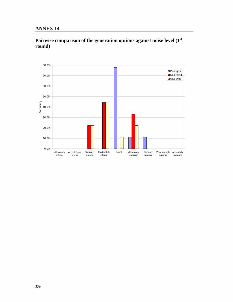
336

ANNEX 14 Pairwise comparison of the generation options against noise level (1st round)

0.0%

10.0%

20.0%

30.0%

40.0%

50.0%

60.0%

70.0%

80.0%

Absolutelyinferior

Very stronglyinferior

Stronglyinferior

Moderatelyinferior


Stronglysuperior

Very stronglysuperior

Absolutelysuperior

Freq

uenc

y


337

ANNEX 15 Pairwise comparison of the generation options against impact on birds and wildlife (1st round)

0.0%

10.0%

20.0%

30.0%

40.0%

50.0%

60.0%

Absolutelyinferior


Stronglyinferior

Moderatelyinferior


Stronglysuperior


Absolutelysuperior

Freq

uenc

y


338

ANNEX 16 Pairwise comparison of the generation options against social acceptance (1st round)

0.0%

10.0%

20.0%

30.0%

40.0%

50.0%

Absolutelyinferior


Stronglyinferior

Moderatelyinferior


Stronglysuperior


Absolutelysuperior

Freq

uenc

y

Coal-gasCoal-wind

339

ANNEX 17 Pairwise comparison of the social criteria (1st round)

0.0%

10.0%

20.0%

30.0%

40.0%

50.0%

60.0%

Absolutelyinferior


Stronglyinferior

Moderatelyinferior


Stronglysuperior


Absolutelysuperior

Visual impact-noise impactVisual impact-impact on birds and wildlifeVisual impact-social aceptanceNoise impact-impact on birds and wildlifeNoise impact-social aceptanceImpact on birds and widlife-social aceptance

340

ANNEX 18 Willingness to pay for lower emissions (1st round)

0.0%

10.0%

20.0%

30.0%

40.0%

50.0%

0% 0%-5% 6%-10% more 10%

Freq

uenc

y (%

)

341

ANNEX 19 Delphi questionnaire (2nd round)

EVALUATION OF THE IMPACTS OF DIFFERENT ALTERNATIVES FOR ELECTRICITY GENERATION

This is a multiple choice questionnaire, where the possible answers will appear when clicking in the grey fields.

Assume the necessity of increasing the available power in about 1000 MW. This may be accomplished by new coal, gas or wind power plants. The possible solutions may be described as follows:

Coal solution Description 2 new coal power plants, one with installed capacity equal to 700 MW and another

one with installed capacity equal to 450 MW. Placement Close to large electricity consumption centres. Characteristics In each power station there will be one chimney 225 m high and one cooling tower.

Each power plant may occupy an area of about 1.5 ha (0.015 km2) and burns imported coal.

Examples Presently two power stations operate in Portugal: one in Sines and another one in Pego. Please find attached a photo of a coal power plant presently operating in Portugal.

Gas solution

Description 2 new combined cycle natural gas power plants, one with installed capacity equal to 660 MW and another one with installed capacity equal to 400 MW.

Placement Close to large electricity consumption centres. Characteristics The 660 MW power station will have two chimneys. The 400 MW power station

will have 1 chimney. All the chimneys will be 80 m high. Each power station will have a cooling tower. Each power station may occupy an area of about 1.5 ha (0.015 km2). It burns imported natural gas.

Examples Presently two CCGT operate in Portugal: one in Ribatejo (Carregado) and another one in Tapada do Outerio (Gondomar). Please find attached a photo of a CCGT power plant presently operating in Portugal.

Wind solution

Description 180 new wind farms, with total installed capacity equal 3800 MW. Placement Spread across the country, but with higher concentration in the inland North hills. Characteristics Each wind farm will have between 8 and 10 turbine, about 65 m high and may

occupy an area of about 2.5 ha (0.25 km2). Examples Presently there are about 1000 turbines operating in the mainland, some examples

may be seen in Marão, Açor, Barroso among many others. Please find attached a photo of a wind power plant presently operating in Portugal.

Comments from the experts: The dimension of the wind farms suggested in the 1st round was excessive, according to the present characteristics of the available machines. The characterization of the wind solution was changed according to the comments received. Please find attached a picture from a more recent wind farm. For the wind solution the installed power must be much higher than the average power needed. Due to wind fluctuations and intermittency, the average available power for electricity production on the wind solution is much lower than the installed power, which does not happen with either the coal or the gas solution.

342

1st quartile: 25% of the responses were equal or less than the category presented. 2nd quartile (median): 50% of the responses were equal or less than the category presented. 3rd quartile: 75% of the responses were equal or less than the category presented.

PART I We ask you now for please make pairwise comparisons of the three solutions with respect to some criteria: 1. Visual impact. This criterion hardly may be quantified and depends heavily on the individual perception. It is associated with the aesthetic aspect, and it will be necessary to assess if the project will bring significant changes to the landscape and if these changes will reduce the visual quality of the region.

d) The visual impact of the coal solution is to the wind solution.

Results from the 1st round: 1st quartile: ”4-moderately inferior” 2nd quartile (median): “6-moderartely superior” 3rd quartile : “7-stronlgy superior”

Your answer to the first round was:

e) The visual impact of the gas solution is to the wind solution.

Results from the 1st round:

1st quartile: ”3- strongly inferior” 2nd quartile (median): “6-moderartely superior” 3rd quartile : “6-moderartely superior”


Comment from the experts: The visual impact of a wind farm may be superior to the other solutions. However, some may assume this as a positive impact because it represents an image of clean energy production. 2. Noise level. This criterion is usually associated with sleeping disorders, interference with learning activities and general annoyance, caused by undesirable noise. It will be necessary to assess if the project will change the noise levels in the region.

a) The noise impact of the coal solution is to the wind solution.

Results from the 1st round: 1st quartile: ”4- moderately inferior” 2nd quartile (median): “4- moderately inferior” 3rd quartile : “6-moderartely superior”


3. Social acceptance. This criterion is associated with the way project will be seen and accepted by the population in general. It may generate some resistance or on the other hand may be considered desirable.

a) The social acceptance of the coal solution is to the wind solution.

343

Results from the 1st round: 1st quartile: ”2- very strongly inferior” 2nd quartile (median): “2- very strongly inferior” 3rd quartile : “4-moderartely inferior”


c) The social acceptance of the gas solution is to the wind solution. (new question)

PART II

We ask you now for please make pairwise comparisons of the importance of the considered criteria:

b) The visual impact is to the impact on birds and wildlife.

Results from the 1st round: 1st quartile: ”3- strongly inferior” 2nd quartile (median): “4- moderately inferior” 3rd quartile : “6-moderartely superior”


c) The visual impact is to the social acceptance.

Results from the 1st round: 1st quartile: between ”3- strongly inferior” and “4- moderately inferior” 2nd quartile (median): “4- moderately inferior” 3rd quartile : “5-equal”


d) The noise level is to the impact on birds and wildlife.

Results from the 1st round: 1st quartile: between ”3- strongly inferior” and “4- moderately inferior” 2nd quartile (median): between “4- moderately inferior” and “5-equal” 3rd quartile : “7- strongly superior”


e) The noise level is to the social acceptance.

Results from the 1st round: 1st quartile: between ”3- strongly inferior” and “4- moderately inferior” 2nd quartile (median): between “4- moderately inferior” and “5-equal” 3rd quartile : “6- moderately superior”


344

PART III In January 2006, the electricity bill paid by an average Portuguese consumer was about 41 €/month (14 centon/kWh) We ask you now for evaluate how much would you be willing to increase your average electricity bill, in order to contribute to the reduction of the atmospheric pollution:

Results from the 1st round: Median: “between 6 and 10%” 22% of the experts selected: “0%” 22% of the experts selected: “up to 5%” 22% of the experts selected: “between 6 and 10%” 22% of the experts selected: “more than 10%”


Contact (email) Comments:

Please send to [email protected]

Thank you for your collaboration!

345

ANNEX 20 Pairwise comparison of the generation options against visual impact (2nd round)

0.0%

10.0%

20.0%

30.0%

40.0%

50.0%

60.0%

Absolutelyinferior

Verystronglyinferior

Stronglyinferior

Moderatelyinferior


Stronglysuperior

Verystronglysuperior

Absolutelysuperior

Freq

uenc

y

coal-windgas-wind

Coal-wind

Rating 1 2 3 4 5 6 7 8 9 Change* 0 0 0 0 0 2 1 0 1 * Absolute difference in number seclecting rating, round 1-2. Net change: 2 Number of participants: 9 Percent change: 22.22%

Gas-wind Rating 1 2 3 4 5 6 7 8 9 Change* 0 0 0 0 0 1 1 0 0 * Absolute difference in number seclecting rating, round 1-2. Net change: 1 Number of participants: 9 Percent change: 11.11%

346

ANNEX 21 Pairwise comparison of the generation options against noise level (1st round)

0.0%

10.0%

20.0%

30.0%

40.0%

50.0%

60.0%

70.0%

80.0%

Absolutelyinferior


Stronglyinferior

Moderatelyinferior


Stronglysuperior


Absolutelysuperior

Freq

uenc

y

coal-wind

Coal-wind Rating 1 2 3 4 5 6 7 8 9 Change* 0 0 1 1 0 0 0 0 0 * Absolute difference in number seclecting rating, round 1-2. Net change: 1 Number of participants: 9 Percent change: 11.11%

347

ANNEX 22 Pairwise comparison of the generation options against social acceptance (2nd round)

0.0%

10.0%

20.0%

30.0%

40.0%

50.0%

Absolutelyinferior


Stronglyinferior

Moderatelyinferior


Stronglysuperior


Absolutelysuperior

Freq

uenc

y

coal-windgas-wind

Coal-wind Rating 1 2 3 4 5 6 7 8 9 Change* 1 0 1 1 0 0 0 0 1 * Absolute difference in number seclecting rating, round 1-2. Net change: 2 Number of participants: 9 Percent change: 22.22%

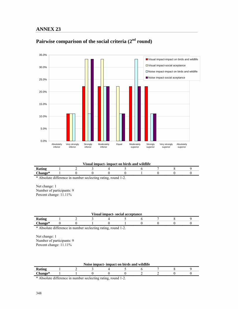
348

ANNEX 23 Pairwise comparison of the social criteria (2nd round)

0.0%

5.0%

10.0%

15.0%

20.0%

25.0%

30.0%

35.0%

Absolutelyinferior


Stronglyinferior

Moderatelyinferior


Stronglysuperior


Absolutelysuperior

Visual impact-impact on birds and wildlife

Visual impact-social aceptance

Noise impact-impact on birds and wildlife

Noise impact-social aceptance

Visual impact- impact on birds and wildlife Rating 1 2 3 4 5 6 7 8 9Change* 1 0 0 0 0 1 0 0 0 * Absolute difference in number seclecting rating, round 1-2. Net change: 1 Number of participants: 9 Percent change: 11.11%

Visual impact- social acceptance Rating 1 2 3 4 5 6 7 8 9 Change* 0 0 1 0 1 0 0 0 0 * Absolute difference in number seclecting rating, round 1-2. Net change: 1 Number of participants: 9 Percent change: 11.11%

Noise impact- impact on birds and wildlife Rating 1 2 3 4 5 6 7 8 9 Change* 1 1 0 0 0 2 2 0 0 * Absolute difference in number seclecting rating, round 1-2.

349

Net change: 3 Number of participants: 9 Percent change: 33.33%

Noise impact- social acceptance Rating 1 2 3 4 5 6 7 8 9 Change* 0 0 1 0 0 1 0 0 0 * Absolute difference in number seclecting rating, round 1-2. Net change: 1 Number of participants: 9 Percent change: 11.11%

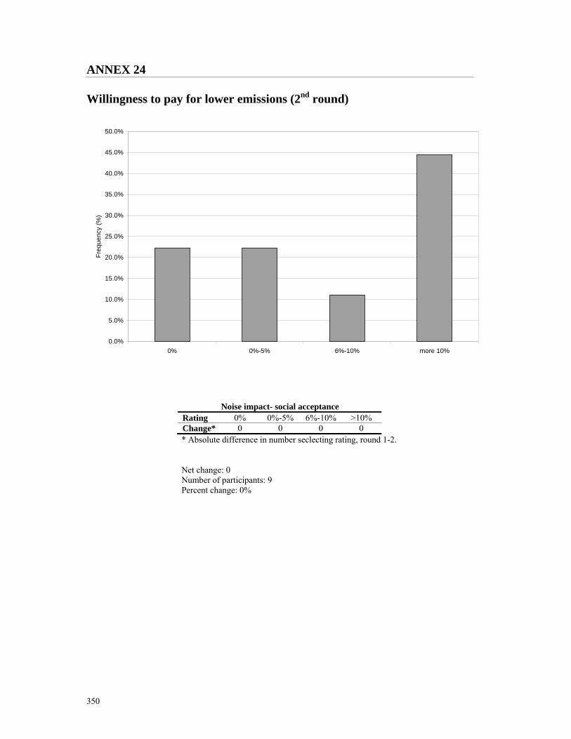
350

ANNEX 24 Willingness to pay for lower emissions (2nd round)

0.0%

5.0%

10.0%

15.0%

20.0%

25.0%

30.0%

35.0%

40.0%

45.0%

50.0%

0% 0%-5% 6%-10% more 10%

Freq

uenc

y (%

)

Noise impact- social acceptance Rating 0% 0%-5% 6%-10% >10% Change* 0 0 0 0 * Absolute difference in number seclecting rating, round 1-2.

Net change: 0 Number of participants: 9 Percent change: 0%

paula fernanda varandas ferreira - universidade do...

Documents