optimal multiprocessor real-time scheduling via … · optimal multiprocessor real-time scheduling...
TRANSCRIPT
PAUL D. E. REGNIER
OPTIMAL MULTIPROCESSOR REAL-TIMESCHEDULING VIA REDUCTION TO
UNIPROCESSOR
Tese apresentada ao Programa Multiinstitucional de
Pós-Graduação em Ciência da Computação da Uni-
versidade Federal da Bahia, Universidade Estadual
de Feira de Santana e Universidade Salvador, como
requisito parcial para obtenção do grau de Doutor
em Ciência da Computação.
Orientador: Prof. Dr. George Marconi de Araujo Lima
Salvador
2012
Sistemas de Bibliotecas - UFBA
Regnier, Paul Denis Etienne.Optimal multiprocessor real-time scheduling via reduction to uniprocessor /
Paul Denis Etienne Regnier. - 2012.143p. : il.
Orientador: Prof. Dr. George Marconi de Araujo Lima.Tese (doutorado) – Programa Multiinstitucional de Pós-Graduação em Ciência
da Computação da Universidade Federal da Bahia em parceria com a UniversidadeEstadual de Feira de Santana e Universidade Salvador, Salvador, 2012.
1. Processamento eletrônico de dados em tempo real. 2. Multiprocessadores.3. Algoritmos. 4. Otimização matemática. 5. Cliente/servidor (Computadores).I. Lima, George Marconi de Araujo. II. Universidade Federal da Bahia.Instituto de Matemática. III. Universidade Estadual de Feira de Santana.IV. Universidade Salvador. V. Título.
CDD - 004.33CDU - 004.415.2.031.43
TERMO DE APROVAÇÃO
PAUL DENIS ETIENNE REGNIER
OPTIMAL MULTIPROCESSOR REAL-TIME SCHEDULING VIAREDUCTION TO UNIPROCESSOR
Esta tese foi julgada adequada à obtenção do títulode Doutor em Ciência da Computação e aprovadaem sua forma final pelo Programa Multiinstitucionalde Pós-Graduação em Ciência da Computação daUFBA-UEFS-UNIFACS.
Salvador, 16 de março de 2012
PROFESSOR E ORIENTADOR GEORGE MARCONI LIMA, PH.D.
Universidade Federal da Bahia
PROFESSOR RÔMULO SILVA DE OLIVEIRA, DR.
Universidade Federal de Santa Catarina
PROFESSOR EDUARDO CAMPONOGARA, PH.D.
Universidade Federal de Santa Catarina
PROFESSOR RAIMUNDO JOSÉ DE ARAÚJO MACÊDO, PH.D.
Universidade Federal da Bahia
PROFESSOR FLÁVIO MORAIS DE ASSIS SILVA,DR.-ING.
Universidade Federal da Bahia

iv

To my daughter Ainá, my son Omin and their loving mother,
Vitória

vi

ACKNOWLEDGEMENTS
Thanks to my advisor, George Marconi Lima, for his support, enthusiasm, and patience. Dur-ing this seven years of Graduate Studies, MSc and finally, PhD, George has been altogethera wonderful adviser as well as a very nice and enthusiast research partner. I have learnt anenormous amount from working with him, and have thoroughly enjoyed doing so. I am alsograteful to him for helping arranging financial support for me throughout my stay at UFBa. Iwould also like to thank Ernesto Massa, PhD student at UFBa, who I worked with very closely.This research would probably not have come up to lightness without their helpful motivationand dedicated participation.
In addition, I would like to thank my committee members Rômulo Silva de Oliveira, Ed-uardo Camponogara, Raimundo José de Araújo Macêdo and Flávio Morais de Assis Silva. Eachcommittee member contributed to my dissertation in different and valuable ways.
Professor Aline Maria Santos Andrade deserves my sincere acknowledgements for its initialencouragement and confidence in my capacity to become a Computer Science researcher.
Over the years, it has been a pleasure to be a graduate student at the computer sciencedepartment at UFBa in large part because of the invaluable contributions of the staff. I thankeach member of the administrative and technical staff for the countless ways they assisted mewhile I was a graduate student. I feel privileged to have had so much support.
Also thanks to my french family who gave me support, education and self-confidence toquit my professional European career and begin a new career of Computer Science researcherat Salvador, Bahia.
Finally, I would like to thank the Brazilian people, their culture and hospitality. In par-ticular, thanks to the guardians of Capoeira, Samba and Candomblé, three traditional culturalquilombos, which are partly responsible for my move from France to Brazil. I am also particu-larly grateful to my friend and debater, Fernando Conceição, professor and radical. It is visitinghim in Salvador, 2003, that I met Vitória, who became my life’s companion. In 2006, at thebeginning of my Master, she gave birth to Omin, our first son and, in 2008, at the beginning ofthis PhD, to Ainá, our first daughter. Thanks to the three of them for their love and patienceduring this long journey to doctorate.
vii

viii ACKNOWLEDGEMENTS
ABSTRACT
Over the last decade, improving the performance of uniprocessor computer systems has beenachieved mainly by increasing operation frequency. Recently such an approach has faced manyphysical limitations such as excessive energy consumption, chip overheating, and memory sizeand memory speed access. To overcome such limitations, the use of replicated hardware compo-nents has become a necessary and practical solution. However, dealing with the concurrency forresources caused by parallel execution of programs in recent multi-core and/or multiprocessorarchitectures has brought about new interesting challenges.
In this dissertation, we focus our attention on the problem of scheduling a set of actions,usually called jobs or tasks, on a multiprocessor system. Moreover, we consider this problemin the context of real-time systems, whose specification contains constraints in both time andvalue domains.
From a synthetic point of view, a real-time system is comprised of three main components:
• A real-time workload, which specifies the tasks that must be executed together with theirtemporal constraints;
• A real-time platform, comprised of a set processors with well-defined properties on whichtasks are executing;
• A scheduling algorithm, in charge of scheduling tasks on the processors of the real-timeplatform.
We are interested here in optimal dynamic priority scheduling algorithms which always finda correct schedule whenever one exists, that is we are interested in algorithms able to schedulesystems with real-time workloads that require up to 100% utilization of the real-time platformprocessors.
Although various optimal solutions exist for uniprocessor systems, those solutions can notbe simply exported to systems with two or more processors. Indeed, for such multiproces-sor systems, the simple fact that a single real-time task can not execute on two processors si-multaneously introduce a dramatic amount of complexity in comparison with the uniprocessorscheduling problem.
Hence, optimal multiprocessor real-time scheduling is challenging. Several solutions haverecently been presented for some specific task model. For instance, the proportionate fairness
(Pfair) approach (BARUAH et al., 1993) has been successfully used as building block of manyoptimal algorithm for the periodic, preemptive and independent task model with implicit dead-lines. However, the Pfair approach enforces deadline equality subdividing the workload of eachtask proportionally to its execution rate and imposing the deadlines of each task on all othertasks (LEVIN et al., 2010). As a consequence, many tasks execute between every two consec-utive system deadlines, possibly leading to more preemptions and migrations than necessary.
As the main contribution of this dissertation, we present RUN (Reduction to UNiproces-sor), a new optimal scheduling algorithm for periodic task set with implicit deadlines, which is
ix
x ABSTRACT
not based on proportionate fairness and that reduces the multiprocessor problem to a series ofuniprocessor problems.
RUN combines two main ideas. First, RUN uses the key concept of idle scheduling. In anutshell, at some instant t, RUN schedules a task τ using both the knowledge of its remainingexecution time as well as its remaining idle time. Since idle and execution time are the twofacets of the same task, we call this scheduling approach duality. This leads us to the Dual
Scheduling Equivalence (DSE), as previously introduced in (REGNIER et al., 2011).
Second, RUN is based on the decrease of the number of tasks to be scheduled by theiraggregation into supertasks, that we call servers, with accumulated rate no greater than one.Each server is responsible for scheduling its set of client tasks, according to some schedulingpolicy.
Combining servers with duality, RUN leads us to the original notion of partitioned pro-
portionate fairness (PP-Fair), which can be viewed as a weak version of proportional fairness.Briefly, under global fairness, each server of a task set T is guaranteed to execute for a timeproportional to the accumulated rate of the tasks in T . As a consequence, the optimality of thescheduling algorithm for a single server, namely Earliest Deadline First (EDF) here, guaranteesthat each client’s job meets its deadline.
In summary, by combining the Dual Scheduling Equivalence and the PP-Fair approach,RUN reduces the problem of scheduling a given task set on m processors to an equivalentproblem of scheduling one or more different task sets on uniprocessor systems. Consequently,RUN significantly outperforms existing optimal algorithms in terms of preemptions with anupper bound of Oplogmq average preemptions per job on m processors. Also, RUN possiblyreduces to Partitioned-EDF whenever a proper partition of the task set into servers can be found.
Keywords: Real-Time Systems, Multiprocessor, Scheduling, Optimality, Server
RESUMO
Durante a última década, o melhoramento do desempenho de sistemas de computadores mono-processador foi principalmente alcançado pelo aumento da freqüência de operação. Recente-mente, essa abordagem tem enfrentado muitas limitações físicas, como o consumo excessivode energia, o superaquecimento dos chips, e a quantidade de memória e velocidade de acesso àmemória. Para superar tais limitações, o uso de componentes de hardware replicados tornou-seuma solução necessária e prática. No entanto, lidar com a concorrência pelo uso dos recursoscausados pela execução paralela de programas em arquiteturas multicores e / ou multiproces-sador recentes gerou novos desafios interessantes.
Nesta dissertação, focamos a nossa atenção sobre o problema do escalonamento de um con-junto de ações, geralmente chamadas de jobs ou tarefas, num sistema multiprocessador. Alémdisso, considera-se este problema no contexto de sistemas de tempo real, cuja especificaçãocontém restrições tanto no domínio do tempo quanto no domínio dos valores.
De um ponto de vista sintético, um sistema de tempo real é constituída por três componentesprincipais:
• A carga de trabalho de tempo real, que especifica as tarefas que devem ser executadasjuntamente com as suas restrições temporais;
• Uma plataforma de tempo real, composto de um conjunto de processador com pro-priedades bem definidas em que as tarefas são executadas;
• Um algoritmo de escalonamento, responsável pelo escalonamento das tarefas sobre osprocessadores da plataforma de tempo real.
Estamos interessados aqui em algoritmos ótimos de escalonamento baseados em prioridadedinâmica, os quais sempre encontram um escalonamento correto quando existe um, ou seja,estamos interessados em algoritmos capazes de escalonar sistemas com cargas de trabalho detempo real requerendo até 100% de utilização dos processadores da plataforma de tempo real.
Embora existam várias soluções ótimas para um sistema monoprocessador, essas soluçõesnão podem ser simplesmente exportadas para sistemas com dois ou mais processadores. Defato, para esses sistemas multiprocessador, o simples fato de que uma tarefa de tempo realnão possa ser executada em dois processadores simultaneamente introduz uma complexidaderelevante em comparação com o problema do escalonamento em um sistema monoprocessador.
Por estas razões, o problema do escalonamento ótimo em sistemas de tempo real multipro-cessador é um grande desafio. Várias soluções têm sido recentemente apresentadas para algunsmodelos específicos de tarefa. Por exemplo, a abordagem justiça proporcional (Proportion-ate Fairness - Pfair) (BARUAH et al., 1993) tem sido utilizada com sucesso como peça chavepara o desenvolvimento de algoritmos ótimos para o modelo de tarefas periódicas, preemptivas,independentes e com deadlines implícitos. No entanto, a abordagem Pfair impõe a igualdadedos deadlines, subdividindo a carga de trabalho de cada tarefa proporcionalmente à sua taxa
xi
xii RESUMO
de execução e impondo os deadlines de cada tarefa para todas as outras tarefas (LEVIN et al.,2010). Como conseqüência, muitas tarefas executam entre cada dois deadlines consecutivos dosistema, levando possivelmente a mais preempções e migrações do que o necessário.
Como principal contribuição desta dissertação, apresentamos RUN (Redução para Unipro-cessor), um novo algoritmo de escalonamento ótimo para conjunto de tarefas periódicas comdeadlines implícitas, não baseado na abordagem de justiça proporcional, que reduz o problemamultiprocessador para uma série de problemas monoprocessador.
RUN combina duas idéias principais. Primeiro, RUN usa o conceito-chave do escalona-mento do tempo ócio. Em suma, em algum instante t, RUN agenda uma tarefa usando tantoo conhecimento de seu tempo de execução restante, bem como o seu tempo ócio restante.Chamamos essa abordagem de escalonamento por dualidade, pois os tempos ócio e de exe-cução são duas facetas complementares de uma mesma tarefa. Isto nos leva ao princípio deEquivalência Dual de Escalonamento, conforme foi previamente introduzido em (REGNIER etal., 2011).
Segundo, RUN baseia-se na diminuição do número de tarefas a ser escalonadas pela suaagregação em supertasks, os quais chamamos de servidores, com taxa acumulada não superiora um. Cada servidor é responsável por escalonar o seu conjunto de tarefas clientes, de acordocom alguma política de escalonamento.
Combinando servidores com dualidade, RUN nos leva à ideia original de justiça propor-
cional particionada (PP-Fair), que pode ser visto como uma versão fraca da justiça propor-cional. Brevemente, de acordo com a justiça global, cada servidor de um conjunto de tarefas T
é garantido de executar por um tempo proporcional à taxa acumulada das tarefas de T . Con-seqüentemente, a otimalidade do algoritmo de escalonamento utilizado por um único servidor,ou seja Earliest Deadline First (EDF) aqui, garante que os jobs de cada cliente cumpre os seusdeadlines.
Em suma, combinando o princípio de Equivalência Dual de Escalonamento e a abordagemPP-Fair, RUN reduz o problema do escalonamento de um certo conjunto de tarefas em m pro-cessadores para o problema equivalente do escalonamento de um ou mais conjuntos de tarefasdiferentes em sistemas monoprocessador. Conseqüentemente, RUN supera significativamenteos algoritmos ótimos existentes em termos de preempções com um limite superior de Oplogmqpreempções média por jobs em m processadores. Além disso, RUN pode se reduzir a EDF-particionado sempre que uma partição adequado das tarefas em servidores pode ser encontrada.
Palavras-chave: Sistemas de Tempo Real, Multiprocessador, Escalonamento, Otimalidade,Servidor
CONTENTS
List of Figures xviii
List of Tables xix
List of Notations xxii
Chapter 1—Introduction 23
1.1 Real-Time Systems . . . . . . . . . . . . . . . . . . . . . . . . . . . . . . . . 24
1.2 Real-Time Workload . . . . . . . . . . . . . . . . . . . . . . . . . . . . . . . 25
1.2.1 Job Model . . . . . . . . . . . . . . . . . . . . . . . . . . . . . . . . 25
1.2.2 Task Model . . . . . . . . . . . . . . . . . . . . . . . . . . . . . . . . 26
1.3 Real-Time Platform . . . . . . . . . . . . . . . . . . . . . . . . . . . . . . . . 27
1.4 Real-Time Scheduling . . . . . . . . . . . . . . . . . . . . . . . . . . . . . . 28
1.4.1 Schedule . . . . . . . . . . . . . . . . . . . . . . . . . . . . . . . . . 28
1.4.2 Scheduling Algorithm . . . . . . . . . . . . . . . . . . . . . . . . . . 31
1.5 Optimality in Real-Time Systems . . . . . . . . . . . . . . . . . . . . . . . . . 32
1.6 Motivation . . . . . . . . . . . . . . . . . . . . . . . . . . . . . . . . . . . . . 33
1.7 Contribution . . . . . . . . . . . . . . . . . . . . . . . . . . . . . . . . . . . . 36
1.8 Structure of this Dissertation . . . . . . . . . . . . . . . . . . . . . . . . . . . 39
Chapter 2—Multiprocessor Scheduling Spectrum 41
2.1 Introduction . . . . . . . . . . . . . . . . . . . . . . . . . . . . . . . . . . . . 41
2.2 Multiprocessor Scheduling Spectrum . . . . . . . . . . . . . . . . . . . . . . . 42
2.3 Simple Algorithms . . . . . . . . . . . . . . . . . . . . . . . . . . . . . . . . 43
2.3.1 McNaughton Algorithm . . . . . . . . . . . . . . . . . . . . . . . . . 43
2.3.2 Global EDF, LLF . . . . . . . . . . . . . . . . . . . . . . . . . . . . . 45
xiii
xiv CONTENTS
2.3.3 EDZL . . . . . . . . . . . . . . . . . . . . . . . . . . . . . . . . . . . 46
2.4 Optimal Multiprocessor Scheduling . . . . . . . . . . . . . . . . . . . . . . . 49
2.4.1 Proportionate Fairness . . . . . . . . . . . . . . . . . . . . . . . . . . 49
2.4.2 Pfair derivatives . . . . . . . . . . . . . . . . . . . . . . . . . . . . . . 50
2.5 An Unfair approach . . . . . . . . . . . . . . . . . . . . . . . . . . . . . . . . 54
2.6 Idle Scheduling . . . . . . . . . . . . . . . . . . . . . . . . . . . . . . . . . . 55
2.6.1 Discussion . . . . . . . . . . . . . . . . . . . . . . . . . . . . . . . . 57
2.7 Conclusion . . . . . . . . . . . . . . . . . . . . . . . . . . . . . . . . . . . . 57
Chapter 3—Tasks and Servers 59
3.1 Introduction . . . . . . . . . . . . . . . . . . . . . . . . . . . . . . . . . . . . 59
3.2 Fixed-Rate Task Model . . . . . . . . . . . . . . . . . . . . . . . . . . . . . . 60
3.3 Fully Utilized System . . . . . . . . . . . . . . . . . . . . . . . . . . . . . . . 61
3.4 Servers . . . . . . . . . . . . . . . . . . . . . . . . . . . . . . . . . . . . . . 63
3.4.1 Server model and notations . . . . . . . . . . . . . . . . . . . . . . . . 63
3.4.2 EDF Server . . . . . . . . . . . . . . . . . . . . . . . . . . . . . . . . 66
3.5 Partial Knowledge . . . . . . . . . . . . . . . . . . . . . . . . . . . . . . . . . 68
3.6 Partitioned Proportionate Fairness . . . . . . . . . . . . . . . . . . . . . . . . 68
3.7 Conclusion . . . . . . . . . . . . . . . . . . . . . . . . . . . . . . . . . . . . 71
Chapter 4—Virtual Scheduling 73
4.1 Introduction . . . . . . . . . . . . . . . . . . . . . . . . . . . . . . . . . . . . 73
4.2 DUAL Operation . . . . . . . . . . . . . . . . . . . . . . . . . . . . . . . . . 74
4.3 PACK Operation . . . . . . . . . . . . . . . . . . . . . . . . . . . . . . . . . 77
4.4 REDUCE Operation . . . . . . . . . . . . . . . . . . . . . . . . . . . . . . . 80
4.5 Conclusion . . . . . . . . . . . . . . . . . . . . . . . . . . . . . . . . . . . . 84
Chapter 5—REDUCTION TO UNIPROCESSOR (RUN) 87
5.1 Introduction . . . . . . . . . . . . . . . . . . . . . . . . . . . . . . . . . . . . 87
5.2 RUN Scheduling . . . . . . . . . . . . . . . . . . . . . . . . . . . . . . . . . 89
5.3 Parallel Execution Requirement . . . . . . . . . . . . . . . . . . . . . . . . . 95
5.4 Conclusion . . . . . . . . . . . . . . . . . . . . . . . . . . . . . . . . . . . . 98
CONTENTS xv
Chapter 6—ASSESSMENT 99
6.1 Introduction . . . . . . . . . . . . . . . . . . . . . . . . . . . . . . . . . . . . 99
6.2 RUN Implementation . . . . . . . . . . . . . . . . . . . . . . . . . . . . . . . 100
6.3 Reduction Complexity . . . . . . . . . . . . . . . . . . . . . . . . . . . . . . 101
6.4 On-line Complexity . . . . . . . . . . . . . . . . . . . . . . . . . . . . . . . . 102
6.5 Preemption Bound . . . . . . . . . . . . . . . . . . . . . . . . . . . . . . . . 103
6.6 Simulation . . . . . . . . . . . . . . . . . . . . . . . . . . . . . . . . . . . . . 108
6.7 Conclusion . . . . . . . . . . . . . . . . . . . . . . . . . . . . . . . . . . . . 111
Chapter 7—CONCLUSION 113
Appendix
Appendix A—Idle Serialization 125
A.1 Frame . . . . . . . . . . . . . . . . . . . . . . . . . . . . . . . . . . . . . . . 125
A.2 Mapping . . . . . . . . . . . . . . . . . . . . . . . . . . . . . . . . . . . . . . 126
A.3 Level . . . . . . . . . . . . . . . . . . . . . . . . . . . . . . . . . . . . . . . 127
A.4 Idle Serialization . . . . . . . . . . . . . . . . . . . . . . . . . . . . . . . . . 128
A.5 On-line scheduling . . . . . . . . . . . . . . . . . . . . . . . . . . . . . . . . 130
Appendix B—EDF Server Theorem: another proof 133
B.1 Scaling . . . . . . . . . . . . . . . . . . . . . . . . . . . . . . . . . . . . . . 133
B.2 Direct Proof of the EDF Server Theorem . . . . . . . . . . . . . . . . . . . . 134
Appendix C—X-RUN: a proposal for sporadic tasks 137
C.1 Task Model . . . . . . . . . . . . . . . . . . . . . . . . . . . . . . . . . . . . 137
C.2 RUN subtree . . . . . . . . . . . . . . . . . . . . . . . . . . . . . . . . . . . 137
C.3 X-RUN: Switching Approach . . . . . . . . . . . . . . . . . . . . . . . . . . . 139
C.4 X-RUN: Budget Estimation . . . . . . . . . . . . . . . . . . . . . . . . . . . . 140
C.4.1 Weighting Approach . . . . . . . . . . . . . . . . . . . . . . . . . . . 140
C.4.2 Horizon Approach . . . . . . . . . . . . . . . . . . . . . . . . . . . . 143

xvi CONTENTS
LIST OF FIGURES
1.1 Execution of a Job . . . . . . . . . . . . . . . . . . . . . . . . . . . . . . . . 25
1.2 Periodic task schedule . . . . . . . . . . . . . . . . . . . . . . . . . . . . . . . 26
1.3 Global EDF deadline miss . . . . . . . . . . . . . . . . . . . . . . . . . . . . 34
1.4 EDZL deadline miss . . . . . . . . . . . . . . . . . . . . . . . . . . . . . . . 35
1.5 Valid schedule . . . . . . . . . . . . . . . . . . . . . . . . . . . . . . . . . . . 35
1.6 Dual Scheduling Equivalence (DSE) . . . . . . . . . . . . . . . . . . . . . . . 37
1.7 RUN global scheduling approach . . . . . . . . . . . . . . . . . . . . . . . . . 39
2.1 McNaughton schedule on 3 processors. . . . . . . . . . . . . . . . . . . . . . 43
2.2 McNaughton proof illustration . . . . . . . . . . . . . . . . . . . . . . . . . . 44
2.3 McNaughton non-working schedule Example . . . . . . . . . . . . . . . . . . 45
2.4 EDZL deadline miss . . . . . . . . . . . . . . . . . . . . . . . . . . . . . . . 47
2.5 EDZL upper bound example . . . . . . . . . . . . . . . . . . . . . . . . . . . 49
2.6 TL-Plane node example . . . . . . . . . . . . . . . . . . . . . . . . . . . . . . 51
2.7 DP-wrap schedule example . . . . . . . . . . . . . . . . . . . . . . . . . . . . 52
2.8 EKG schedule example . . . . . . . . . . . . . . . . . . . . . . . . . . . . . . 54
2.9 EDF map examples. . . . . . . . . . . . . . . . . . . . . . . . . . . . . . . . . 56
2.10 Minimum and Maximum ISM examples . . . . . . . . . . . . . . . . . . . . . 56
3.1 Fixed-rate task schedule . . . . . . . . . . . . . . . . . . . . . . . . . . . . . 61
3.2 A two-server set. The notation Xpρq means that ρpXq “ ρ. . . . . . . . . . . . 64
3.3 Valid schedule of a server whose client miss its deadline . . . . . . . . . . . . 65
3.4 Valid schedule of an EDF-server . . . . . . . . . . . . . . . . . . . . . . . . . 65
3.5 Budget management and schedule of an EDF-server . . . . . . . . . . . . . . . 66
3.6 External scheduling constraints . . . . . . . . . . . . . . . . . . . . . . . . . . 69
3.7 Partitioned Proportionate Fairness Approach . . . . . . . . . . . . . . . . . . . 70
3.8 Proportionate Fairness Approach . . . . . . . . . . . . . . . . . . . . . . . . . 70
xvii
xviii LIST OF FIGURES
4.1 Dual Scheduling Equivalence (DSE) . . . . . . . . . . . . . . . . . . . . . . . 74
4.2 Packing example of Γ “ tS1, S2, . . . , S7u . . . . . . . . . . . . . . . . . . . 78
4.3 Packing and PACK operation example of Γ “ tS1, S2, . . . , S7u . . . . . . . . . 79
4.4 Packing, PACK operation, and duality example of Γ “ tS1, S2, . . . , S7u . . . . 81
5.1 RUN tree example . . . . . . . . . . . . . . . . . . . . . . . . . . . . . . . . . 90
5.2 RUN tree example . . . . . . . . . . . . . . . . . . . . . . . . . . . . . . . . . 90
5.3 RUN schedule example . . . . . . . . . . . . . . . . . . . . . . . . . . . . . . 91
5.4 RUN Tree Scheduling rule example . . . . . . . . . . . . . . . . . . . . . . . 91
5.5 RUN tree example . . . . . . . . . . . . . . . . . . . . . . . . . . . . . . . . . 93
5.6 RUN schedule example . . . . . . . . . . . . . . . . . . . . . . . . . . . . . . 94
5.7 RUN subtree example . . . . . . . . . . . . . . . . . . . . . . . . . . . . . . . 96
5.8 Subtree tree example . . . . . . . . . . . . . . . . . . . . . . . . . . . . . . . 97
6.1 A dual JRE . . . . . . . . . . . . . . . . . . . . . . . . . . . . . . . . . . . . . 105
6.2 Two Preemptions from one job release . . . . . . . . . . . . . . . . . . . . . . 106
6.3 Fraction of task sets requiring 1 and 2 reduction levels . . . . . . . . . . . . . 112
6.4 Migrations- and preemptions-per-job varying the processor number . . . . . . 112
6.5 Preemptions per job varying utilization . . . . . . . . . . . . . . . . . . . . . . 112
A.1 EDF map examples. . . . . . . . . . . . . . . . . . . . . . . . . . . . . . . . . 127
A.2 History map and maximum ISM . . . . . . . . . . . . . . . . . . . . . . . . . 129
A.3 Minimum and maximum ISM comparison . . . . . . . . . . . . . . . . . . . . 131
A.4 Minimum and Maximum ISM examples . . . . . . . . . . . . . . . . . . . . . 132
B.1 Deadline miss case 1 . . . . . . . . . . . . . . . . . . . . . . . . . . . . . . . 135
B.2 Deadline miss case 2 . . . . . . . . . . . . . . . . . . . . . . . . . . . . . . . 136
C.1 RUN subtree example . . . . . . . . . . . . . . . . . . . . . . . . . . . . . . . 138
C.2 Switching between WCS and RUN . . . . . . . . . . . . . . . . . . . . . . . . 140
C.3 The Continuity Argument . . . . . . . . . . . . . . . . . . . . . . . . . . . . . 141
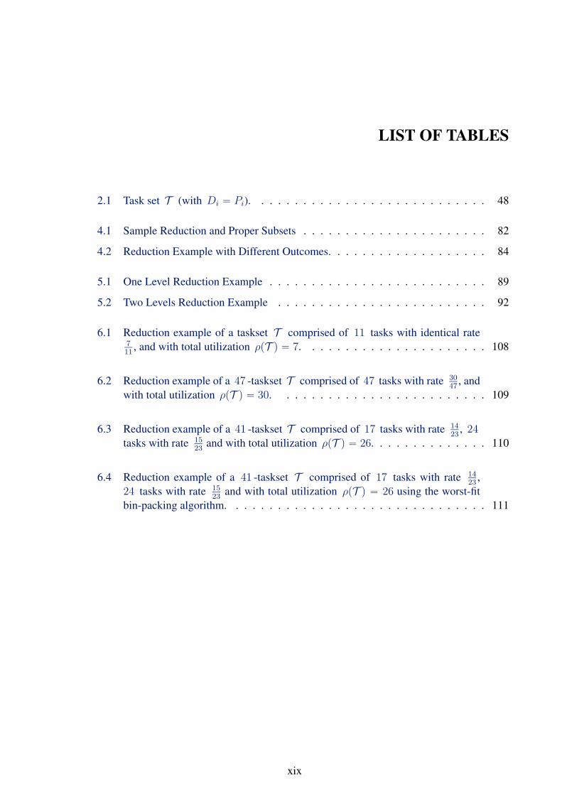
LIST OF TABLES
2.1 Task set T (with Di “ Pi). . . . . . . . . . . . . . . . . . . . . . . . . . . . 48
4.1 Sample Reduction and Proper Subsets . . . . . . . . . . . . . . . . . . . . . . 82
4.2 Reduction Example with Different Outcomes. . . . . . . . . . . . . . . . . . . 84
5.1 One Level Reduction Example . . . . . . . . . . . . . . . . . . . . . . . . . . 89
5.2 Two Levels Reduction Example . . . . . . . . . . . . . . . . . . . . . . . . . 92
6.1 Reduction example of a taskset T comprised of 11 tasks with identical rate7
11, and with total utilization ρpT q “ 7. . . . . . . . . . . . . . . . . . . . . . 108
6.2 Reduction example of a 47 -taskset T comprised of 47 tasks with rate 30
47, and
with total utilization ρpT q “ 30. . . . . . . . . . . . . . . . . . . . . . . . . 109
6.3 Reduction example of a 41 -taskset T comprised of 17 tasks with rate 14
23, 24
tasks with rate 15
23and with total utilization ρpT q “ 26. . . . . . . . . . . . . . 110
6.4 Reduction example of a 41 -taskset T comprised of 17 tasks with rate 14
23,
24 tasks with rate 15
23and with total utilization ρpT q “ 26 using the worst-fit
bin-packing algorithm. . . . . . . . . . . . . . . . . . . . . . . . . . . . . . . 111
xix

xx LIST OF TABLES
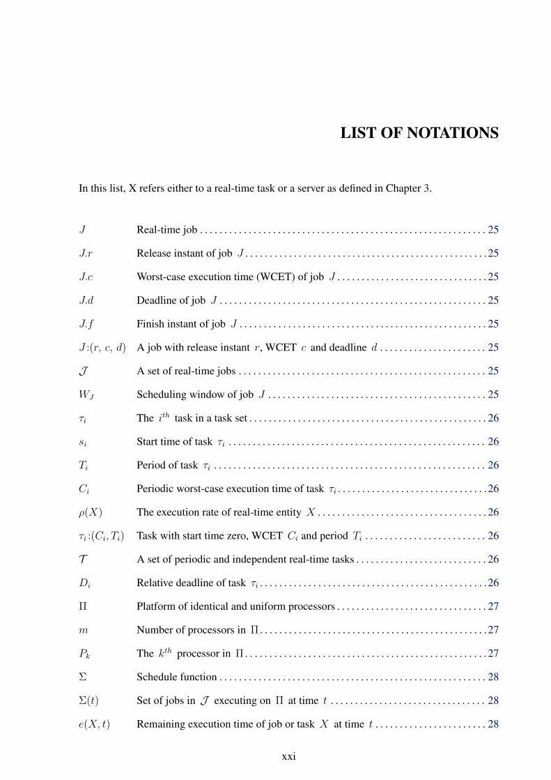
LIST OF NOTATIONS
In this list, X refers either to a real-time task or a server as defined in Chapter 3.
J Real-time job . . . . . . . . . . . . . . . . . . . . . . . . . . . . . . . . . . . . . . . . . . . . . . . . . . . . . . . . . . . 25
J.r Release instant of job J . . . . . . . . . . . . . . . . . . . . . . . . . . . . . . . . . . . . . . . . . . . . . . . . . .25
J.c Worst-case execution time (WCET) of job J . . . . . . . . . . . . . . . . . . . . . . . . . . . . . . . 25
J.d Deadline of job J . . . . . . . . . . . . . . . . . . . . . . . . . . . . . . . . . . . . . . . . . . . . . . . . . . . . . . . 25
J.f Finish instant of job J . . . . . . . . . . . . . . . . . . . . . . . . . . . . . . . . . . . . . . . . . . . . . . . . . . . 25
J :pr, c, dq A job with release instant r, WCET c and deadline d . . . . . . . . . . . . . . . . . . . . . . 25
J A set of real-time jobs . . . . . . . . . . . . . . . . . . . . . . . . . . . . . . . . . . . . . . . . . . . . . . . . . . . 25
WJ Scheduling window of job J . . . . . . . . . . . . . . . . . . . . . . . . . . . . . . . . . . . . . . . . . . . . . 25
τi The ith task in a task set . . . . . . . . . . . . . . . . . . . . . . . . . . . . . . . . . . . . . . . . . . . . . . . . . 26
si Start time of task τi . . . . . . . . . . . . . . . . . . . . . . . . . . . . . . . . . . . . . . . . . . . . . . . . . . . . . 26
Ti Period of task τi . . . . . . . . . . . . . . . . . . . . . . . . . . . . . . . . . . . . . . . . . . . . . . . . . . . . . . . . 26
Ci Periodic worst-case execution time of task τi . . . . . . . . . . . . . . . . . . . . . . . . . . . . . . .26
ρpXq The execution rate of real-time entity X . . . . . . . . . . . . . . . . . . . . . . . . . . . . . . . . . . . 26
τi :pCi, Tiq Task with start time zero, WCET Ci and period Ti . . . . . . . . . . . . . . . . . . . . . . . . . 26
T A set of periodic and independent real-time tasks . . . . . . . . . . . . . . . . . . . . . . . . . . . 26
Di Relative deadline of task τi . . . . . . . . . . . . . . . . . . . . . . . . . . . . . . . . . . . . . . . . . . . . . . .26
Π Platform of identical and uniform processors . . . . . . . . . . . . . . . . . . . . . . . . . . . . . . . 27
m Number of processors in Π . . . . . . . . . . . . . . . . . . . . . . . . . . . . . . . . . . . . . . . . . . . . . . .27
Pk The kth processor in Π . . . . . . . . . . . . . . . . . . . . . . . . . . . . . . . . . . . . . . . . . . . . . . . . . . 27
Σ Schedule function . . . . . . . . . . . . . . . . . . . . . . . . . . . . . . . . . . . . . . . . . . . . . . . . . . . . . . . 28
Σptq Set of jobs in J executing on Π at time t . . . . . . . . . . . . . . . . . . . . . . . . . . . . . . . . 28
epX, tq Remaining execution time of job or task X at time t . . . . . . . . . . . . . . . . . . . . . . . 28
xxi
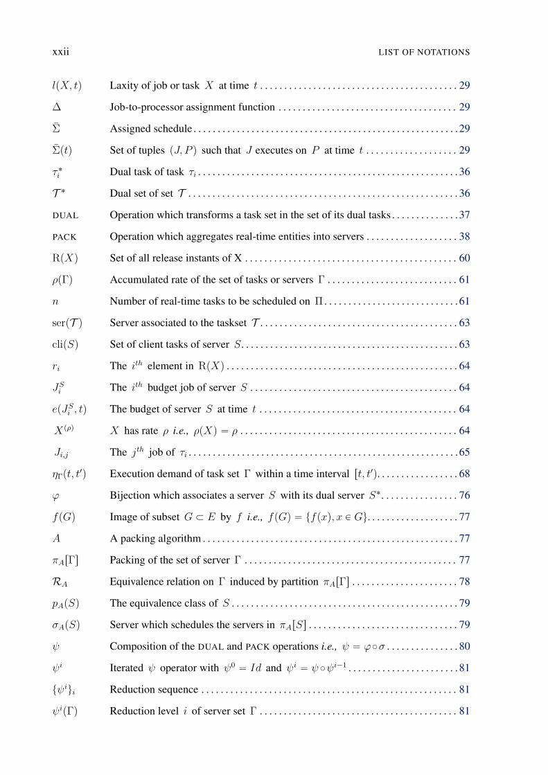
xxii LIST OF NOTATIONS
lpX, tq Laxity of job or task X at time t . . . . . . . . . . . . . . . . . . . . . . . . . . . . . . . . . . . . . . . . . 29
∆ Job-to-processor assignment function . . . . . . . . . . . . . . . . . . . . . . . . . . . . . . . . . . . . . 29
Σ Assigned schedule . . . . . . . . . . . . . . . . . . . . . . . . . . . . . . . . . . . . . . . . . . . . . . . . . . . . . . .29
Σptq Set of tuples pJ, P q such that J executes on P at time t . . . . . . . . . . . . . . . . . . . 29
τ˚i Dual task of task τi . . . . . . . . . . . . . . . . . . . . . . . . . . . . . . . . . . . . . . . . . . . . . . . . . . . . . . 36
T ˚ Dual set of set T . . . . . . . . . . . . . . . . . . . . . . . . . . . . . . . . . . . . . . . . . . . . . . . . . . . . . . . . 36
DUAL Operation which transforms a task set in the set of its dual tasks . . . . . . . . . . . . . . 37
PACK Operation which aggregates real-time entities into servers . . . . . . . . . . . . . . . . . . . 38
RpXq Set of all release instants of X . . . . . . . . . . . . . . . . . . . . . . . . . . . . . . . . . . . . . . . . . . . . 60
ρpΓq Accumulated rate of the set of tasks or servers Γ . . . . . . . . . . . . . . . . . . . . . . . . . . . 61
n Number of real-time tasks to be scheduled on Π . . . . . . . . . . . . . . . . . . . . . . . . . . . . 61
serpT q Server associated to the taskset T . . . . . . . . . . . . . . . . . . . . . . . . . . . . . . . . . . . . . . . . . 63
clipSq Set of client tasks of server S. . . . . . . . . . . . . . . . . . . . . . . . . . . . . . . . . . . . . . . . . . . . . 63
ri The ith element in RpXq . . . . . . . . . . . . . . . . . . . . . . . . . . . . . . . . . . . . . . . . . . . . . . . . 64
JSi The ith budget job of server S . . . . . . . . . . . . . . . . . . . . . . . . . . . . . . . . . . . . . . . . . . . 64
epJSi , tq The budget of server S at time t . . . . . . . . . . . . . . . . . . . . . . . . . . . . . . . . . . . . . . . . . 64
Xpρq X has rate ρ i.e., ρpXq “ ρ . . . . . . . . . . . . . . . . . . . . . . . . . . . . . . . . . . . . . . . . . . . . . 64
Ji,j The jth job of τi . . . . . . . . . . . . . . . . . . . . . . . . . . . . . . . . . . . . . . . . . . . . . . . . . . . . . . . .65
ηΓpt, t1q Execution demand of task set Γ within a time interval rt, t1q. . . . . . . . . . . . . . . . . 68
ϕ Bijection which associates a server S with its dual server S˚. . . . . . . . . . . . . . . . 76
fpGq Image of subset G Ă E by f i.e., fpGq “ tfpxq, x P Gu. . . . . . . . . . . . . . . . . . . 77
A A packing algorithm . . . . . . . . . . . . . . . . . . . . . . . . . . . . . . . . . . . . . . . . . . . . . . . . . . . . . 77
πArΓs Packing of the set of server Γ . . . . . . . . . . . . . . . . . . . . . . . . . . . . . . . . . . . . . . . . . . . . 77
RA Equivalence relation on Γ induced by partition πArΓs . . . . . . . . . . . . . . . . . . . . . . 78
pApSq The equivalence class of S . . . . . . . . . . . . . . . . . . . . . . . . . . . . . . . . . . . . . . . . . . . . . . . 79
σApSq Server which schedules the servers in πArSs . . . . . . . . . . . . . . . . . . . . . . . . . . . . . . . 79
ψ Composition of the DUAL and PACK operations i.e., ψ “ ϕ˝σ . . . . . . . . . . . . . . . 80
ψi Iterated ψ operator with ψ0 “ Id and ψi “ ψ ˝ψi´1 . . . . . . . . . . . . . . . . . . . . . . . 81
tψiui Reduction sequence . . . . . . . . . . . . . . . . . . . . . . . . . . . . . . . . . . . . . . . . . . . . . . . . . . . . . 81
ψipΓq Reduction level i of server set Γ . . . . . . . . . . . . . . . . . . . . . . . . . . . . . . . . . . . . . . . . . 81
Chapter
1A real-time system is an information processing system which has to respond to externally generated input stimuli
within a finite and specified period: the correctness depends not only on the logical result but also on the time it
was delivered; the failure to respond is as bad as the wrong response.
Alan Burns and Andy Wellings, 2009
INTRODUCTION
Over the last decade, improving the performance of uniprocessor computer systems has been
achieved mainly by increasing operation frequency. Recently such an approach has faced many
physical limitations such as excessive energy consumption, chip overheating, and memory size
and memory speed access. To overcome such limitations, the use of replicated hardware com-
ponents has become a necessary and practical solution. However, the organization of the con-
current use of hardware components by parallel software programs is a challenging task which
requires further investigation.
Indeed, dealing with the concurrency for resources caused by parallel execution of pro-
grams in recent multi-core and/or multiprocessor architectures has brought about new interest-
ing challenges. For instance, memory sharing must be organized to ensure data consistency
between different levels of cache and memory. Also, the organization of communication be-
tween the various hardware components must take competition for resources into account with-
out compromising aspects related to timeliness or throughput. In this context, the scheduling of
processes or threads must be optimized to ensure correctness and efficient resource usage.
This dissertation focuses on the problem of scheduling a set of actions, usually called jobs
or tasks, on a multiprocessor system. More specifically, we consider this problem in the context
of real-time systems, whose specification contains constraints in both time and value domains.
23
24 INTRODUCTION
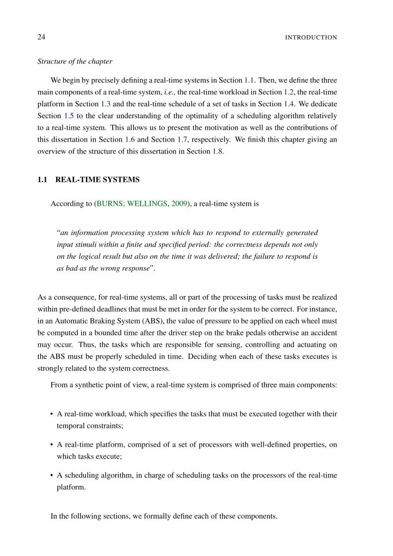
Structure of the chapter
We begin by precisely defining a real-time systems in Section 1.1. Then, we define the three
main components of a real-time system, i.e., the real-time workload in Section 1.2, the real-time
platform in Section 1.3 and the real-time schedule of a set of tasks in Section 1.4. We dedicate
Section 1.5 to the clear understanding of the optimality of a scheduling algorithm relatively
to a real-time system. This allows us to present the motivation as well as the contributions of
this dissertation in Section 1.6 and Section 1.7, respectively. We finish this chapter giving an
overview of the structure of this dissertation in Section 1.8.
1.1 REAL-TIME SYSTEMS
According to (BURNS; WELLINGS, 2009), a real-time system is
“an information processing system which has to respond to externally generated
input stimuli within a finite and specified period: the correctness depends not only
on the logical result but also on the time it was delivered; the failure to respond is
as bad as the wrong response”.
As a consequence, for real-time systems, all or part of the processing of tasks must be realized
within pre-defined deadlines that must be met in order for the system to be correct. For instance,
in an Automatic Braking System (ABS), the value of pressure to be applied on each wheel must
be computed in a bounded time after the driver step on the brake pedals otherwise an accident
may occur. Thus, the tasks which are responsible for sensing, controlling and actuating on
the ABS must be properly scheduled in time. Deciding when each of these tasks executes is
strongly related to the system correctness.
From a synthetic point of view, a real-time system is comprised of three main components:
• A real-time workload, which specifies the tasks that must be executed together with their
temporal constraints;
• A real-time platform, comprised of a set of processors with well-defined properties, on
which tasks execute;
• A scheduling algorithm, in charge of scheduling tasks on the processors of the real-time
platform.
In the following sections, we formally define each of these components.
1.2 REAL-TIME WORKLOAD 25
J J
J.r
J.d
J.f
δ1 δ2
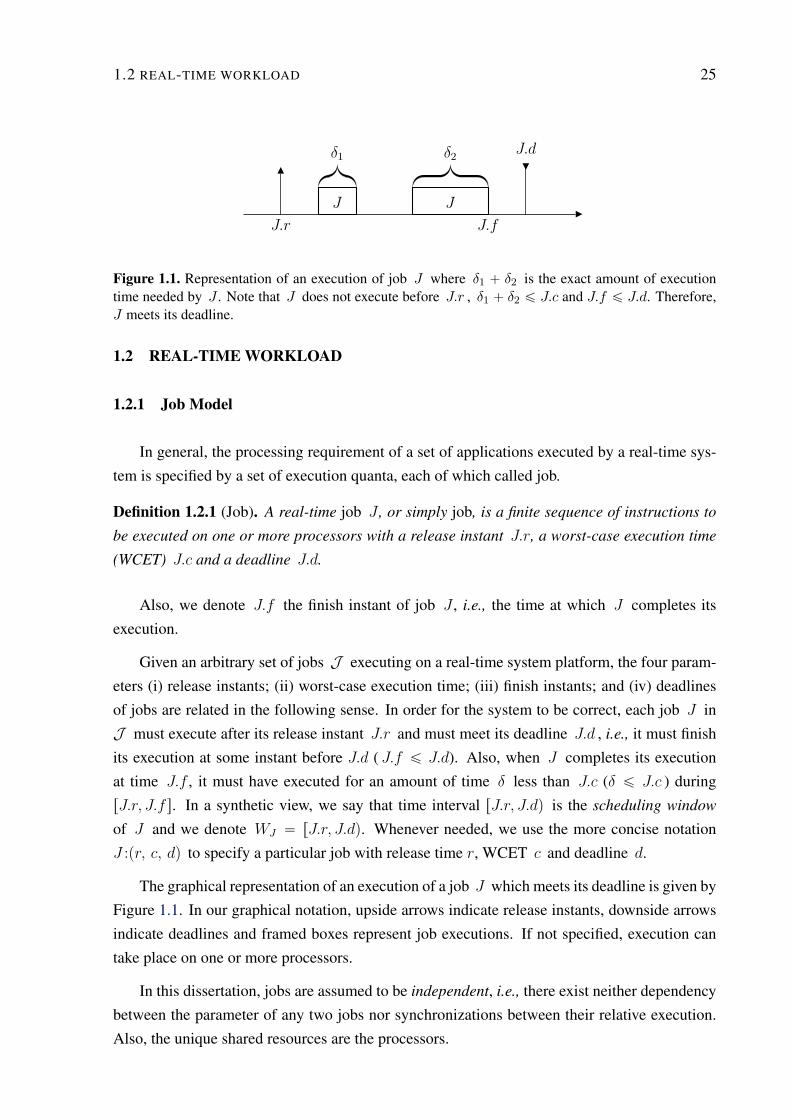
Figure 1.1. Representation of an execution of job J where δ1 ` δ2 is the exact amount of executiontime needed by J . Note that J does not execute before J.r , δ1 ` δ2 ď J.c and J.f ď J.d. Therefore,J meets its deadline.
1.2 REAL-TIME WORKLOAD
1.2.1 Job Model
In general, the processing requirement of a set of applications executed by a real-time sys-
tem is specified by a set of execution quanta, each of which called job.
Definition 1.2.1 (Job). A real-time job J , or simply job, is a finite sequence of instructions to
be executed on one or more processors with a release instant J.r, a worst-case execution time
(WCET) J.c and a deadline J.d.
Also, we denote J.f the finish instant of job J , i.e., the time at which J completes its
execution.
Given an arbitrary set of jobs J executing on a real-time system platform, the four param-
eters (i) release instants; (ii) worst-case execution time; (iii) finish instants; and (iv) deadlines
of jobs are related in the following sense. In order for the system to be correct, each job J in
J must execute after its release instant J.r and must meet its deadline J.d , i.e., it must finish
its execution at some instant before J.d ( J.f ď J.d). Also, when J completes its execution
at time J.f , it must have executed for an amount of time δ less than J.c (δ ď J.c ) during
rJ.r, J.f s. In a synthetic view, we say that time interval rJ.r, J.dq is the scheduling window
of J and we denote WJ “ rJ.r, J.dq. Whenever needed, we use the more concise notation
J :pr, c, dq to specify a particular job with release time r, WCET c and deadline d.
The graphical representation of an execution of a job J which meets its deadline is given by
Figure 1.1. In our graphical notation, upside arrows indicate release instants, downside arrows
indicate deadlines and framed boxes represent job executions. If not specified, execution can
take place on one or more processors.
In this dissertation, jobs are assumed to be independent, i.e., there exist neither dependency
between the parameter of any two jobs nor synchronizations between their relative execution.
Also, the unique shared resources are the processors.
26 INTRODUCTION
0 1 2 3 4 5 6
J1 J2
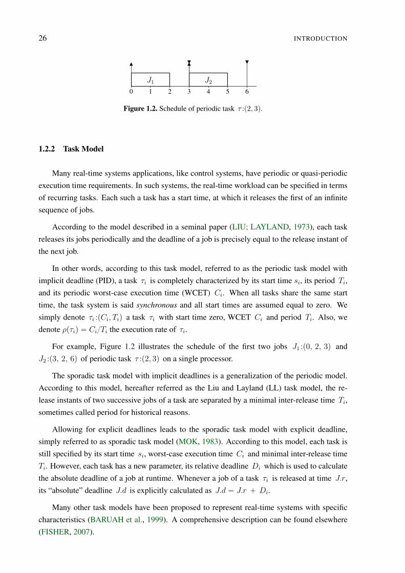
Figure 1.2. Schedule of periodic task τ :p2, 3q.
1.2.2 Task Model
Many real-time systems applications, like control systems, have periodic or quasi-periodic
execution time requirements. In such systems, the real-time workload can be specified in terms
of recurring tasks. Each such a task has a start time, at which it releases the first of an infinite
sequence of jobs.
According to the model described in a seminal paper (LIU; LAYLAND, 1973), each task
releases its jobs periodically and the deadline of a job is precisely equal to the release instant of
the next job.
In other words, according to this task model, referred to as the periodic task model with
implicit deadline (PID), a task τi is completely characterized by its start time si, its period Ti,
and its periodic worst-case execution time (WCET) Ci. When all tasks share the same start
time, the task system is said synchronous and all start times are assumed equal to zero. We
simply denote τi :pCi, Tiq a task τi with start time zero, WCET Ci and period Ti. Also, we
denote ρpτiq “ CiTi the execution rate of τi.
For example, Figure 1.2 illustrates the schedule of the first two jobs J1 :p0, 2, 3q and
J2 :p3, 2, 6q of periodic task τ :p2, 3q on a single processor.
The sporadic task model with implicit deadlines is a generalization of the periodic model.
According to this model, hereafter referred as the Liu and Layland (LL) task model, the re-
lease instants of two successive jobs of a task are separated by a minimal inter-release time Ti,
sometimes called period for historical reasons.
Allowing for explicit deadlines leads to the sporadic task model with explicit deadline,
simply referred to as sporadic task model (MOK, 1983). According to this model, each task is
still specified by its start time si, worst-case execution time Ci and minimal inter-release time
Ti. However, each task has a new parameter, its relative deadline Di which is used to calculate
the absolute deadline of a job at runtime. Whenever a job of a task τi is released at time J.r,
its “absolute” deadline J.d is explicitly calculated as J.d “ J.r ` Di.
Many other task models have been proposed to represent real-time systems with specific
characteristics (BARUAH et al., 1999). A comprehensive description can be found elsewhere
(FISHER, 2007).
1.3 REAL-TIME PLATFORM 27
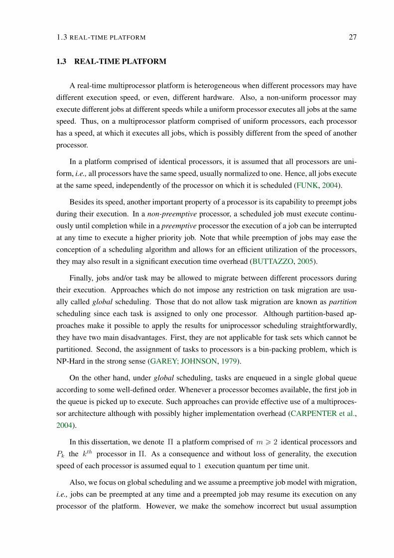
1.3 REAL-TIME PLATFORM
A real-time multiprocessor platform is heterogeneous when different processors may have
different execution speed, or even, different hardware. Also, a non-uniform processor may
execute different jobs at different speeds while a uniform processor executes all jobs at the same
speed. Thus, on a multiprocessor platform comprised of uniform processors, each processor
has a speed, at which it executes all jobs, which is possibly different from the speed of another
processor.
In a platform comprised of identical processors, it is assumed that all processors are uni-
form, i.e., all processors have the same speed, usually normalized to one. Hence, all jobs execute
at the same speed, independently of the processor on which it is scheduled (FUNK, 2004).
Besides its speed, another important property of a processor is its capability to preempt jobs
during their execution. In a non-preemptive processor, a scheduled job must execute continu-
ously until completion while in a preemptive processor the execution of a job can be interrupted
at any time to execute a higher priority job. Note that while preemption of jobs may ease the
conception of a scheduling algorithm and allows for an efficient utilization of the processors,
they may also result in a significant execution time overhead (BUTTAZZO, 2005).
Finally, jobs and/or task may be allowed to migrate between different processors during
their execution. Approaches which do not impose any restriction on task migration are usu-
ally called global scheduling. Those that do not allow task migration are known as partition
scheduling since each task is assigned to only one processor. Although partition-based ap-
proaches make it possible to apply the results for uniprocessor scheduling straightforwardly,
they have two main disadvantages. First, they are not applicable for task sets which cannot be
partitioned. Second, the assignment of tasks to processors is a bin-packing problem, which is
NP-Hard in the strong sense (GAREY; JOHNSON, 1979).
On the other hand, under global scheduling, tasks are enqueued in a single global queue
according to some well-defined order. Whenever a processor becomes available, the first job in
the queue is picked up to execute. Such approaches can provide effective use of a multiproces-
sor architecture although with possibly higher implementation overhead (CARPENTER et al.,
2004).
In this dissertation, we denote Π a platform comprised of m ě 2 identical processors and
Pk the kth processor in Π. As a consequence and without loss of generality, the execution
speed of each processor is assumed equal to 1 execution quantum per time unit.
Also, we focus on global scheduling and we assume a preemptive job model with migration,
i.e., jobs can be preempted at any time and a preempted job may resume its execution on any
processor of the platform. However, we make the somehow incorrect but usual assumption
28 INTRODUCTION
that preemption and migration take zero time. In an actual system, measured preemption and
migration overheads can be accommodated by adjusting the execution requirements of tasks.
1.4 REAL-TIME SCHEDULING
1.4.1 Schedule
Given a set of of jobs (or tasks) J to be executed on platform Π, a schedule of J on
Π usually specifies which jobs of J execute on which processor of Π at all times during
the system execution. However, since we assume a multiprocessor platform Π comprised of
m ě 2 identical processors, we adopt a slightly different definition for a schedule.
In this dissertation, we distinguish two nested steps for a scheduling procedure at some
scheduling instant t, namely the scheduling step and the assigning step.
Scheduling Step
In the scheduling step, which always precedes the assigning step, a subset J 1 of jobs in J
is chosen to execute.
Definition 1.4.1 (Schedule). For any set of jobs J on a platform of m ě 1 identical and
uniform processors, a schedule Σ is a function from all non-negative times t to the power set
of J such that Σptq is the subset of jobs in J executing at time t.
Within an executing schedule Σ, epJ, tq denotes the maximum work remaining for job J
at time t, so that epJ, tq equals J.c minus the amount of time that J has already executed as
of time t. Whenever no confusion is introduced doing so, we also denote epτ, tq the remaining
execution time of task τ at time t. Formally, if 1lΣptq is the indicator function of Σptq defined
by
1lΣptqpJq “
$
’
&
’
%
1 if J P Σptq
0 otherwise
then, the execution requirement of a job J at time t can be expressed as
epJ, tq “ J.c ´
ż t
J.r
1lΣpuqpJqdu
Some assumptions apply to schedules in order for the system to be legal. First, a job can neither
execute prior its release instant nor after its finishing instant. Second, there can be no more jobs
executing than processors at any time, or, in other words, a processor can not execute more than
one job at any time. We summarize those restrictions in the following definition:
1.4 REAL-TIME SCHEDULING 29
Definition 1.4.2 (Legal Schedule). The schedule Σ of a set of jobs J on a platform Π of
m ě 1 processors is legal if it satisfies the following:
(i) If a job J is scheduled at time t (J P Σptq), then the release instant of J is not after t
(J.r ď t) and the remaining execution time of J at t is greater than zero (epJ, tq ą 0);
(ii) No more than m jobs execute at any time, i.e., |Σptq| ď m for all t.
Note that this definition of a legal schedule also holds when J is specified as a recurrent
task system T as stated in Definition 1.2.2.
The laxity of job J , denoted lpJ, tq is defined as the maximum time that the execution
of job can be delayed without compromising its correct completion by its deadline. Formally,
lpJ, tq “ J.d´t´epJ, tq. Whenever no confusion is introduced doing so, we also denote lpτ, tq
the laxity of task τ at time t.
Assigning Step
In this step, the jobs chosen to execute at time t are allocated to processors in Π.
Definition 1.4.3 (Assignment). For any set of jobs J on a platform Π of m identical proces-
sors, an assignment function ∆ assigns a job scheduled at time t to a processor in Π.
We define an assigned schedule, denoted Σ, as the composition of the schedule function
Σ with an assignment function ∆ (Σ “ ∆˝Σ). Formally, at any non-negative time t, Σptq is
the set of tuples pJ, P q with J P J and P P Π such that J executes on P at time t.
Note that an assigned schedule corresponds to the usual definition of schedule. However,
we find it convenient to separate both scheduling and assigning steps since this will allow for a
more concise description of our original scheduling approach.
Also, since processors are identical and since migration is allowed with no penalty, the job-
to-processor assignment function can be considered as an implementation problem which can
be solved straightforwardly according to some previously established goal. In Chapter 6, we
present an assignment procedure devised to minimize preemptions.
Considering a legal schedule Σ, then the following restriction must be satisfied by the
assignment function ∆ in order for the system to be legal: a job can only execute on a single
processor at any time. We state this restriction as follows:
Definition 1.4.4 (Legal Assigned Schedule). Let Σ be a legal schedule of a set of jobs J on a
platform Π of m ě 1 processors. Then, the assigned schedule Σ, composition of Σ with an
assignment ∆, is legal if for any two tuples pJ, P q and pJ 1, P 1q in Σptq, J “ J 1 if and only if
P “ P 1.
30 INTRODUCTION
It is important to emphasize that this latter restriction, which states that there must be no
parallel execution of the same job on different processors, is the main restriction specific to
multiprocessor systems compared to uniprocessor systems. As a matter of fact,
the simple fact that a task can use only one processor even when several processors
are free at the same time adds a surprising amount of difficulty to the scheduling of
multiple processors.
as already stated by (LIU, 1969) as quoted in (BARUAH, 2001).
In this dissertation, we only consider “legal” assignment, according to which, given a legal
schedule as input, a legal assigned schedule is produced as output. It is easy to see that there
always exists such a legal assignment. Indeed, since a legal schedule chooses no more than m
jobs to execute at any time, a simple “legal” assignment is one which allocates a single job per
processor at any time in an arbitrary manner. Thus, in the remainder of the dissertation, we will
omit the assignment step whenever no confusion is introduced doing so.
Among the legal schedules of a job set, we further distinguish those schedules of interest
for real-time systems i.e., schedules in which all jobs meet their deadlines.
Definition 1.4.5 (Valid Schedule). A legal schedule Σ of a job set J is valid if all jobs in J
meet their deadlines, i.e., if for all J in J , J.f ď J.d.
The problem of generating valid schedules of an arbitrary job set on a real-time platform
Π raises two different questions. First, given an arbitrary job set J , is it feasible, i.e., is there
a valid schedule of J on Π? This decision problem, referred to as the feasibility problem,
is known to be NP-complete for arbitrary job sets (GAREY; JOHNSON, 1979). However, a
simple feasibility criterion may be found for specific task/job models. For instance, for a set of
jobs J generated by a set of periodic tasks T “ tτ1, . . . , τnu with execution time Ci , period
Ti and implicit deadlines, it was shown by (LIU; LAYLAND, 1973) that
nÿ
i“1
ρpτiq ď 1
is a sufficient and necessary feasibility condition of J on a single processor. This result was
later extended to identical multiprocessor platform (HORN, 1974; BARUAH, 2001) meaning
thatn
ÿ
i“1
ρpτiq ď m
is a sufficient and necessary feasibility condition of J on a platform comprised of m identical
processors.
The second question, referred to as the scheduling problem can be expressed as follows.
Assuming that J is feasible on Π, is it possible to devise a scheduling algorithm, say SA,
1.4 REAL-TIME SCHEDULING 31
that produces a valid schedule of J on Π? And, having devised SA, is it possible to find a
schedulability criterion which allows to decide whether another different job set is schedulable
by SA?
In general, the answer to this question is hard and sometimes negative. However, solutions
to both problems are known for some specific classes of task sets.
1.4.2 Scheduling Algorithm
Definition 1.4.6. A scheduling algorithm is a procedure which admits a set of jobs J as input
and produces a legal schedule Σ as output.
A scheduling algorithm is work-conserving, or alternatively, non-idling, if it never idles the
processor whenever there exist some jobs ready to execute in the system.
Definition 1.4.7 (Schedulability). A task set T is schedulable by a scheduling algorithm A if
the legal schedule Σ of T by A is valid, i.e., if all tasks in T meets their deadlines in Σ.
Definition 1.4.8 (Feasibility). A task set T is feasible if T is schedulable by some scheduling
algorithm.
Depending on the task and system model, i.e., the set of assumptions about jobs, tasks and
the relying multiprocessor system adopted, different scheduling approaches can be investigated.
For instance, according to the periodic task model, all release time and deadlines are completely
specified before the execution of the system. As a consequence, it is possible to find a valid
schedule of the system off-line, i.e., before its execution. Such a schedule can then be easily
implemented at execution time through a table-driven algorithm.
However, such an off-line scheduling approach may be impracticable when part or all of the
specification of the system is only known at execution time. This is the case, for instance, when
release instants are not known before the execution of the system, as in the sporadic model.
Also, the explicit deadline of a job may be only known at its release instant. In those systems
partly specified, an on-line scheduling procedure is required in order to decide which jobs must
execute on which processor at any time.
In general, a scheduling algorithm makes its choices based on the relative value of some
parameter, used to define the priority of the jobs. When the priority of each job is calculated (or
pre-set) in advance and remains fixed during the whole operation of the system, the scheduling
policy is said to have static priority. For instance, the rate-monotonic scheduling algorithm
(RM) proposed in (LIU; LAYLAND, 1973) is a static priority algorithm which defines the
priority of a job as the inverse of the period of its generating task. Thus, jobs of tasks with
lower periods turn to have higher priorities. Although such a priority policy has the advantage
32 INTRODUCTION
of simplicity and allows for an off-line table-driven approach, it fails to produce a valid schedule
of some feasible task set.
Another class of scheduling algorithms uses dynamic priorities for jobs defined at execu-
tion time. For instance, the Deadline Algorithm, also proposed in (LIU; LAYLAND, 1973)
and nowadays best known as Earliest Deadline First (EDF) algorithm, is a dynamic priority
algorithm according to which the priority of a job is inversely proportional to the value of its
absolute deadline. Thus, jobs with earlier deadlines have higher priorities than jobs with later
deadlines.
As discussed in (BUTTAZZO, 2005), an off-line fixed-priority algorithm, like rate-mono-
tonic, has the advantages of implementation simplicity and low runtime overhead. On the other
hand, dynamic on-line priority algorithms like EDF usually achieve a better utilization of pro-
cessors.
In this dissertation, we focus our attention on those latter dynamic on-line priority algo-
rithms which achieve a full utilization of the processors. However, even if we assume a fully
preemptive and migrating task model, we are interested in algorithms with low preemptions and
migrations overheads.
1.5 OPTIMALITY IN REAL-TIME SYSTEMS
As previously discussed, the description of real-time systems is done through a set of as-
sumptions upon the real-time workload and the multiprocessor platform. This set of assump-
tions defines a model of the system and allows for eventually proving interesting properties for
some particular class of scheduling algorithms.
Among those properties, one of the most relevant and considered is the optimality of the
scheduling algorithm, precisely defined as follows.
Definition 1.5.1. A scheduling algorithm is said to be optimal regarding a real-time system
model if it can produce a valid schedule for any feasible real-time job set possibly specified in
this model.
In the realm of uniprocessor systems, many optimal algorithms are know regarding the dif-
ferent task model described in Section 1.2.2. For example, the optimality of the EDF dynamic
priority algorithm regarding the periodic, preemptive and synchronous task model with implicit
deadlines is proved in (LIU; LAYLAND, 1973), since it achieves full-utilization of the sys-
tem, as mentioned in Section 1.2.2. The optimality result upon EDF was later extended to the
sporadic job model, for both preemptive and not preemptive systems by (DERTOUZOS, 1974;
GEORGE et al., 1996).
The least laxity first (LLF) algorithm proposed by (MOK, 1983) is another example of
1.6 MOTIVATION 33
optimal uniprocessor algorithm for sporadic task model when preemption is allowed. However,
the LLF algorithm has the drawbacks to require a possibly infinite number of preemptions under
a continuous time model (HOLMAN, 2004).
In a recent work, a characterization of all possible on-line preemptive scheduling algorithm
on one processor is given (UTHAISOMBUT, 2008). However, it is still an open problem to
determine whether a similar characterization can be found for optimal algorithms on platforms
comprised of two or more processors. As a matter of fact, it has been known since the end of the
eighties that no optimal on-line algorithm exists when considering a platform comprised of two
or more processors for an arbitrary collection of independent jobs when deadlines and release
times are not known a priori (HONG; LEUNG, 1988; DERTOUZOS; MOK, 1989). This result
was recently extended to the sporadic task model (FISHER et al., 2010). However, optimality
can be achieved for multiprocessor preemptive systems for more restrictive task model, like the
LL model for instance.
Since there exists no on-line optimal algorithm for the sporadic job model, the weaker
notion of suboptimality was introduced by (CHO et al., 2002).
Definition 1.5.2. A preemptive algorithm is suboptimal if it successfully schedules any feasible
set of ready jobs, where a ready job at time t is a job that has been released at or before t .
For instance, the Least Laxity First (LLF) algorithm is suboptimal (DERTOUZOS; MOK,
1989) on any number of processors.
1.6 MOTIVATION
Considering that the multicore / multiprocessor revolution as described in (BERTOGNA,
2007) is an overwhelming reality and since real-time systems are nowadays present in a wide
variety of fields, such as control systems, environmental monitoring, avionic and automotive ap-
plications, there exists a need to extend well-established solutions to the feasibility and schedul-
ing problems in uniprocessor systems to multiprocessor systems. However, the real-time mul-
tiprocessor scheduling problem is commonly acknowledged to be much more complex than
the real-time uniprocessor scheduling problem. Indeed, multiprocessor scheduling solutions
tend to be computationally more expensive and complicated than those used for uniprocessor
scheduling.
A straightforward approach to export uniprocessor scheduling results to multiprocessor
scheduling systems consists in partitioning the task set by statically assigning each task to a
static and single processor. In such an approach, each processor has a fixed set of tasks al-
located to it during the execution of the system. As a consequence, no migration of jobs is
necessary and the multiprocessor scheduling problem is reduced to m uniprocessor schedul-
34 INTRODUCTION
0 1 2 3 4 5 6
J1,1
J2,1
J1,2
J2,2
J3,1 J3,1
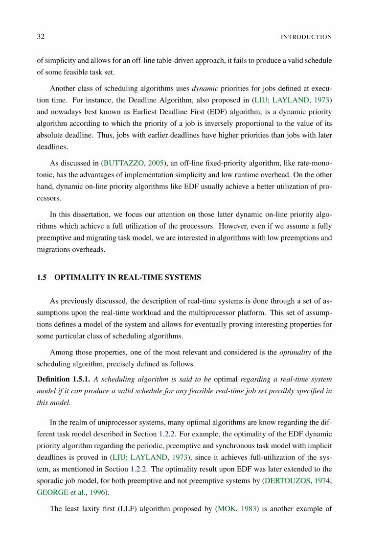
Figure 1.3. Assuming a partitioned approach or global EDF scheduling, the first job J3,1 of τ3 missesits deadline 6.
ing problems. Although elegant and practical, partitioned approaches have the drawbacks of
achieving a low utilization of the system, guaranteeing only 50% utilization in the worst case
(KOREN et al., 1998).
On the other hand, global scheduling approaches can achieve full utilization by migrating
tasks between processors, at the cost of increased runtime overhead. For example, consider a
3-task set T “ tτ1 :p2, 3q, τ2 :p2, 3q, τ3 :p4, 6qu to be schedule on a two-processor system. Since
3ÿ
i“1
ρpτiq “ 2
T is feasible on two processors.
However, if the jobs of tasks τ1 and τ2 are first scheduled on the two processors and run to
completion, then the third task cannot complete on time, as illustrated in Figure 1.3 where Ji,k
is the kth job of task τi. For instance, this would be the case in a partitioned approach or using
global EDF. Indeed, global EDF schedules the earliest deadline job sorted from a single global
queue on a processor whenever it becomes idle.
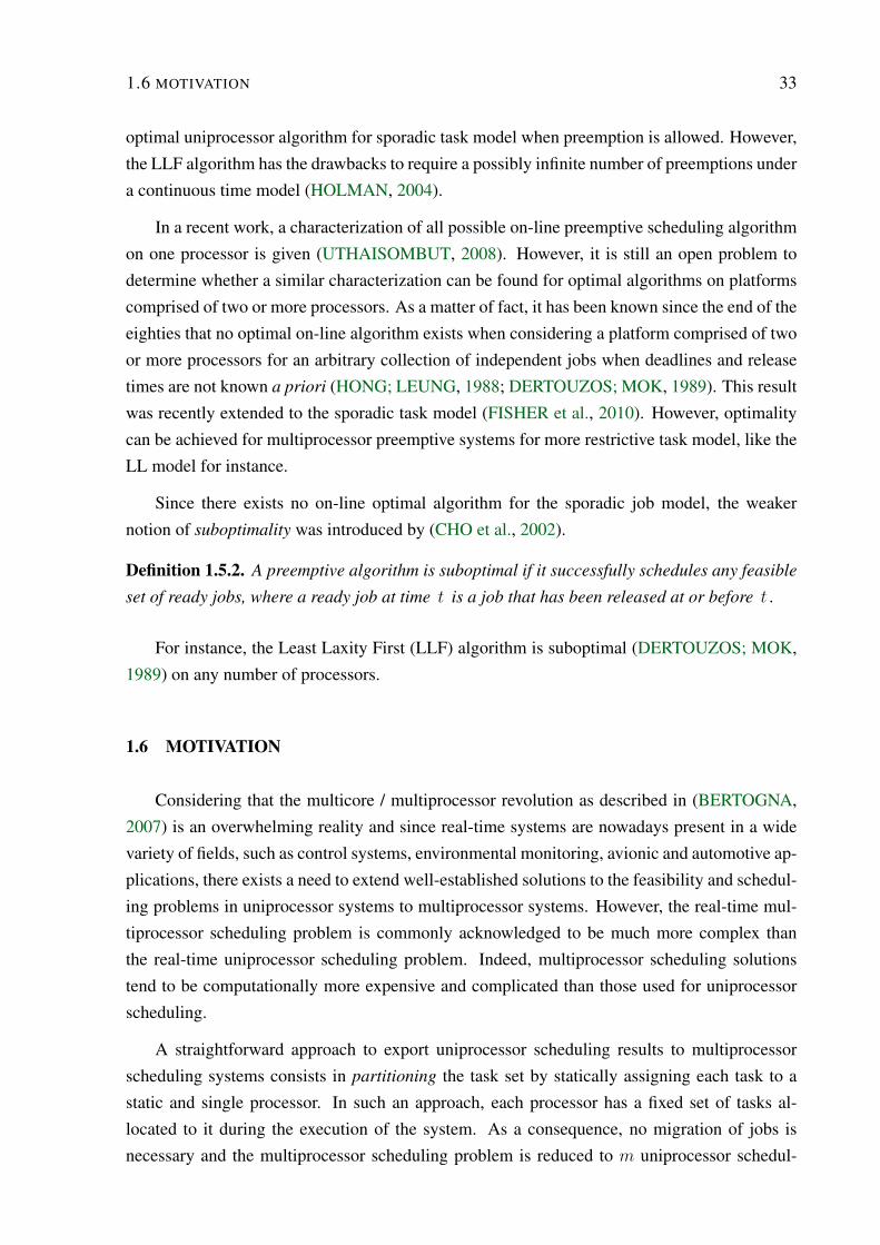
If tasks are allowed to migrate, even global EDZL, which raises the priority of a zero-
laxity job to the highest priority in the system (CHO et al., 2002), would fail to schedule this
simple task set as illustrated in Figure 1.4. Indeed, until time 3, no job reaches zero-laxity.
As a consequence, J1,1 and J2,1 which both have earliest deadline 3 at time 0 are scheduled
continuously during interval r0, 2q. Also, by the non-parallel execution constraint, J3,1 can
only execute on one of the two processors during r2, 3q and an idle slot occurs on one processor
during time interval r2, 3q. When J3,1 reaches zero-laxity at time 3, the idle slot already have
happened and either J1,2 or J2,2 misses its deadline at time 6.
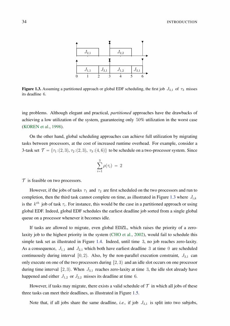
However, if tasks may migrate, there exists a valid schedule of T in which all jobs of these
three tasks can meet their deadlines, as illustrated in Figure 1.5.
Note that, if all jobs share the same deadline, i.e., if job J3,1 is split into two subjobs,
1.6 MOTIVATION 35
0 1 2 3 4 5 6
J1,1
J2,1 J1,2 J2,2
J3,1 J3,1
Figure 1.4. Under EDZL, either job J1,2 of τ1 or job J2,2 of τ2 misses its deadline 6.
0 1 2 3 4 5 6
J1,1 J2,1
J3,1J2,1
J1,2 J2,2
J3,1J2,2
Figure 1.5. A valid schedule produced by a global scheduling approach with migration.
each of which with execution time 2 and deadlines 3 and 6 , then the valid schedule shown
in Figure 1.5 is a simple example of McNaughton’s wrap-around algorithm (MCNAUGHTON,
1959).
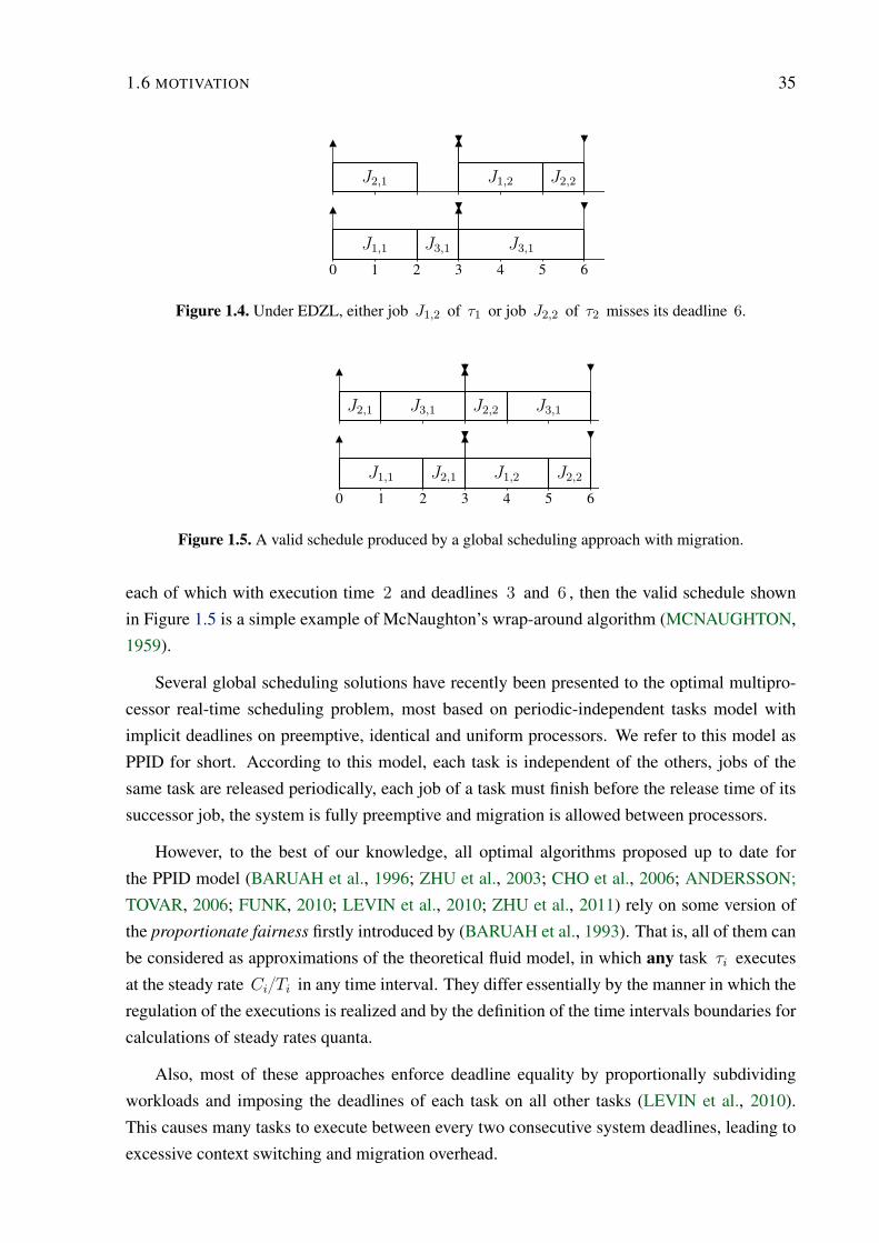
Several global scheduling solutions have recently been presented to the optimal multipro-
cessor real-time scheduling problem, most based on periodic-independent tasks model with
implicit deadlines on preemptive, identical and uniform processors. We refer to this model as
PPID for short. According to this model, each task is independent of the others, jobs of the
same task are released periodically, each job of a task must finish before the release time of its
successor job, the system is fully preemptive and migration is allowed between processors.
However, to the best of our knowledge, all optimal algorithms proposed up to date for
the PPID model (BARUAH et al., 1996; ZHU et al., 2003; CHO et al., 2006; ANDERSSON;
TOVAR, 2006; FUNK, 2010; LEVIN et al., 2010; ZHU et al., 2011) rely on some version of
the proportionate fairness firstly introduced by (BARUAH et al., 1993). That is, all of them can
be considered as approximations of the theoretical fluid model, in which any task τi executes
at the steady rate CiTi in any time interval. They differ essentially by the manner in which the
regulation of the executions is realized and by the definition of the time intervals boundaries for
calculations of steady rates quanta.
Also, most of these approaches enforce deadline equality by proportionally subdividing
workloads and imposing the deadlines of each task on all other tasks (LEVIN et al., 2010).
This causes many tasks to execute between every two consecutive system deadlines, leading to
excessive context switching and migration overhead.
36 INTRODUCTION
1.7 CONTRIBUTION
Assumptions
We consider a real-time platform Π comprised of m ě 2 identical and uniform processors,
each of which executing jobs at a speed of 1 execution quantum per time unit and we focus on
global scheduling.
Also, we assume a preemptive and independent job model with free migration, i.e., jobs
can be preempted at any time and a preempted job may resume its execution instantaneously on
another processor of the platform, with no penalty.
We address a generalization of the PPID model with the goal of finding an optimal on-line
and global scheduling algorithm.
Contribution 1
As a first contribution, we introduce the notion of Dual Scheduling Equivalence (DSE)
in (REGNIER et al., 2011) which is a generalization of (LEVIN et al., 2009). To the best
of our knowledge, this work is the first to propose an optimal multiprocessor algorithm based
on an efficient use of the DSE approach to ensuring the non-parallel execution of tasks in a
multiprocessor real-time system.
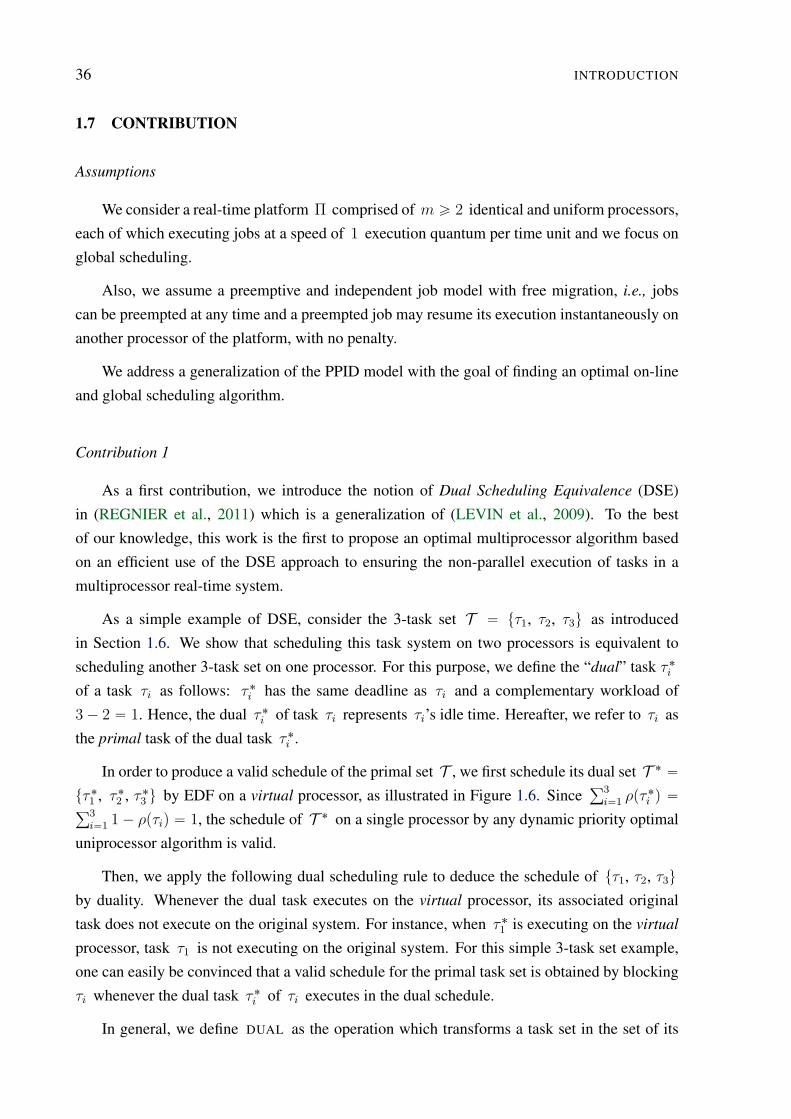
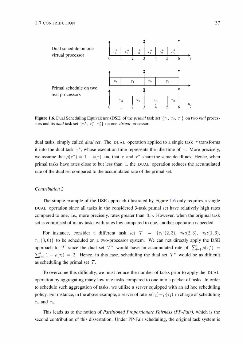
As a simple example of DSE, consider the 3-task set T “ tτ1, τ2, τ3u as introduced
in Section 1.6. We show that scheduling this task system on two processors is equivalent to
scheduling another 3-task set on one processor. For this purpose, we define the “dual” task τ˚i
of a task τi as follows: τ˚i has the same deadline as τi and a complementary workload of
3 ´ 2 “ 1. Hence, the dual τ˚i of task τi represents τi’s idle time. Hereafter, we refer to τi as
the primal task of the dual task τ˚i .
In order to produce a valid schedule of the primal set T , we first schedule its dual set T ˚ “
tτ˚1
, τ˚2
, τ˚3
u by EDF on a virtual processor, as illustrated in Figure 1.6. Sinceř
3
i“1ρpτ˚
i q “ř
3
i“11 ´ ρpτiq “ 1, the schedule of T ˚ on a single processor by any dynamic priority optimal
uniprocessor algorithm is valid.
Then, we apply the following dual scheduling rule to deduce the schedule of tτ1, τ2, τ3u
by duality. Whenever the dual task executes on the virtual processor, its associated original
task does not execute on the original system. For instance, when τ˚1
is executing on the virtual
processor, task τ1 is not executing on the original system. For this simple 3-task set example,
one can easily be convinced that a valid schedule for the primal task set is obtained by blocking
τi whenever the dual task τ˚i of τi executes in the dual schedule.
In general, we define DUAL as the operation which transforms a task set in the set of its
1.7 CONTRIBUTION 37
0 1 2 3 4 5 6 7
Dual schedule on onevirtual processor
τ˚1
τ˚2
τ˚3
τ˚1
τ˚2
τ˚3
Primal schedule on tworeal processors
0 1 2 3 4 5 6 7
τ3
τ2
τ2
τ1
τ3
τ2
τ2
τ1
Figure 1.6. Dual Scheduling Equivalence (DSE) of the primal task set tτ1, τ2, τ3u on two real proces-sors and its dual task set tτ˚
1, τ˚
2τ˚3
u on one virtual processor.
dual tasks, simply called dual set. The DUAL operation applied to a single task τ transforms
it into the dual task τ˚, whose execution time represents the idle time of τ . More precisely,
we assume that ρpτ˚q “ 1 ´ ρpτq and that τ and τ˚ share the same deadlines. Hence, when
primal tasks have rates close to but less than 1, the DUAL operation reduces the accumulated
rate of the dual set compared to the accumulated rate of the primal set.
Contribution 2
The simple example of the DSE approach illustrated by Figure 1.6 only requires a single
DUAL operation since all tasks in the considered 3-task primal set have relatively high rates
compared to one, i.e., more precisely, rates greater than 0.5. However, when the original task
set is comprised of many tasks with rates low compared to one, another operation is needed.
For instance, consider a different task set T “ tτ1 :p2, 3q, τ2 :p2, 3q, τ3 :p1, 6q,
τ4 :p3, 6qu to be scheduled on a two-processor system. We can not directly apply the DSE
approach to T since the dual set T ˚ would have an accumulated rate ofř
4
i“1ρpτ˚
i q “ř
4
i“11 ´ ρpτiq “ 2. Hence, in this case, scheduling the dual set T ˚ would be as difficult
as scheduling the primal set T .
To overcome this difficulty, we must reduce the number of tasks prior to apply the DUAL
operation by aggregating many low rate tasks compared to one into a packet of tasks. In order
to schedule such aggregation of tasks, we utilize a server equipped with an ad hoc scheduling
policy. For instance, in the above example, a server of rate ρpτ3q`ρpτ4q in charge of scheduling
τ3 and τ4.
This leads us to the notion of Partitioned Proportionate Fairness (PP-Fair), which is the
second contribution of this dissertation. Under PP-Fair scheduling, the original task system is
38 INTRODUCTION
partitioned into subsets of accumulated utilization no greater than one by a PACK operation.
Scheduling of tasks in each packed subset is managed in an isolated manner by a virtual server
which globally executes at a steady rate between any two deadlines of its clients, namely those
tasks it serves, according to some own scheduling policy. The system is partitioned proportion-
ate fair in the sense that each server is guaranteed to execute at a fixed rate which is precisely
equal to the sum of the rates of its clients.
However, differently from previous approaches, servers are not required to schedule their
clients at a steady rate. In this dissertation, we only consider EDF-servers which schedule their
clients by Earliest Deadline First (EDF). As a consequence of the schedule isolation of tasks
by servers, a task may essentially cause preemption or migration of another client of the same
server it is attended by. The remaining relatively “rare” preemptions/migrations are due to the
DSE approach which is used to ensure the non-parallel execution of servers.
Contribution 3
We now enunciate our third and primary contribution as the thesis of this dissertation
Optimal on-line algorithm for scheduling periodic and independent real-time tasks
with implicit deadlines on a platform of m ě 2 preemptive, uniform and identi-
cal processors can be built upon Partitioned Proportionate Fairness (PP-Fair) and
Dual Scheduling Equivalence (DSE) approaches. An example of such algorithm,
called RUN, is exhibited in this dissertation with the following properties.
• By performing a sequence of PACK and DUAL operations, RUN reduces the
problem of scheduling a given task set on m processors to an equivalent
problem of scheduling one or more different task sets on uniprocessor systems.
• RUN significantly outperforms existing optimal algorithms in terms of pre-
emptions with an upper bound of Oplogmq average preemptions per job on
m processors.
• RUN reduces to Partitioned-EDF whenever a proper partitioning is found.
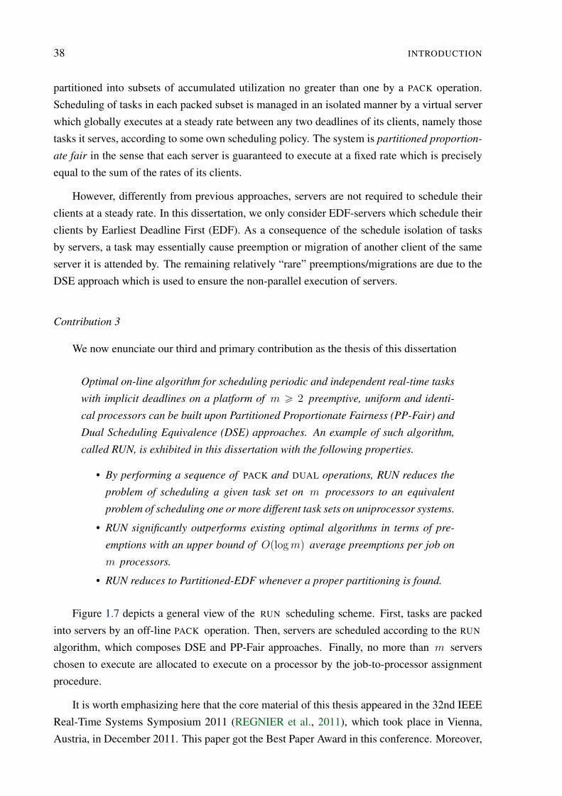
Figure 1.7 depicts a general view of the RUN scheduling scheme. First, tasks are packed
into servers by an off-line PACK operation. Then, servers are scheduled according to the RUN
algorithm, which composes DSE and PP-Fair approaches. Finally, no more than m servers
chosen to execute are allocated to execute on a processor by the job-to-processor assignment
procedure.
It is worth emphasizing here that the core material of this thesis appeared in the 32nd IEEE
Real-Time Systems Symposium 2011 (REGNIER et al., 2011), which took place in Vienna,
Austria, in December 2011. This paper got the Best Paper Award in this conference. Moreover,

1.8 STRUCTURE OF THIS DISSERTATION 39
PACK
DUAL&
PACK
DSE&
EDF
JOB-TO-PROCESSOR
ASSIGNMENTτ0
τ1
τ2
τ3
τ4
τ5
τ6
τ7
τn
S0
S1
S2
SN
UNI-PROCESSOR
SYSTEMS
U
OFF-LINE REDUCTION ON-LINE SCHEDULING
EDF
U
Sk0
Sk1
Sk2
Skm
π0
π1
π2
πm
Figure 1.7. RUN: a global scheduling approach using PACK and DUAL operations and job-to-processorassignment.
an extended version of this paper has been invited to be submitted to the Springer Real-Time
Systems journal.
1.8 STRUCTURE OF THIS DISSERTATION
Equipped with the theoretical background given in this chapter, we follow with an overview
of the state of the art of the multiprocessor real-time scheduling field in Chapter 2, focusing
mainly on global and optimal scheduling solutions.
In Chapter 3, we describe the task model adopted in this dissertation and we define the
server abstraction, first cornerstone of the RUN algorithm, which is used to aggregate low rate
task in order to reduce the total number of tasks to be scheduled.
Chapter 4 depicts the virtual scheduling approach by packing and duality. In particular, the
Dual Scheduling Equivalence, second cornerstone of the RUN algorithm, is established. Finally,
it is shown how a sequence of reduction by packing and duality transforms a multiprocessor task
system into a set of uniprocessor task systems.
Chapter 5 is dedicated to the description of the Reduction to Uniprocessor on-line proce-
dure, the associated on-line scheduling rules and the correctness of the overall RUN algorithm.
In particular, the optimality of the RUN algorithm for periodic task set with implicit deadlines
is established.
40 INTRODUCTION
A theoretical upper bound for the average number of preemptions and migrations per job is
given in Chapter 6, as well as the results of extended comparisons via simulations of RUN with
many other optimal multiprocessor scheduling algorithms.
Chapter 7 concludes this dissertation, introducing some perspectives for future works.
Chapter
2Most of the complexity of multiprocessor real-time scheduling comes from the impossibility for a task to execute
simultaneously on more than one processor. To surround this restriction and achieve optimality for periodic tasks
with implicit deadlines, most solutions proposed until now are based on proportionate fairness. However, the idle
scheduling idea has shown to be another way toward optimality.
MULTIPROCESSOR SCHEDULING SPECTRUM
2.1 INTRODUCTION
In the realm of uniprocessor, assuming a periodic or sporadic task model with implicit
deadline as stated in Definition 1.2.2, the Earliest Deadline First (EDF) and Least Deadline First
(LLF) algorithms are optimal scheduling algorithms (LIU; LAYLAND, 1973; DERTOUZOS,
1974; GEORGE et al., 1996). Moreover, a characterization of all possible on-line preemptive
scheduling algorithm on one processor is given in (UTHAISOMBUT, 2008). However, it is
still an open problem whether a similar characterization can be found for optimal algorithm on
platform comprised of two or more processors.
In fact, as previously stated in Section 1.5 of Chapter 1, it is known that no optimal on-
line algorithm exists when considering a platform comprised of two or more processors for
the sporadic task model (SAHNI, 1979; HONG; LEUNG, 1988; DERTOUZOS; MOK, 1989;
FISHER et al., 2010) with constrained deadlines. However, optimality can be achieved for
multiprocessor preemptive systems for more restrictive task models, like the LL model for
instance.
Structure of the chapter
We begin this Chapter by a brief description of different approaches for multiprocessor
scheduling of real-time tasks on identical processors in Section 2.2. Then, we present in Sec-
tion 2.3, some of the main simple global scheduling algorithms developed to date. In Sec-
tions 2.4 and 2.5, we focus our attention on most of the solutions known at the present time
41
42 MULTIPROCESSOR SCHEDULING SPECTRUM
which lead to optimality for periodic real-time tasks with implicit deadlines. Before to briefly
conclude this chapter with Section 2.7, we give a glimpse of the idle scheduling approach in
Section 2.6, the guiding idea which has led us, ultimately, to the finding of the RUN algorithm.
2.2 MULTIPROCESSOR SCHEDULING SPECTRUM
The spectrum of the real-time multiprocessor scheduling algorithms can be characterized
according to the way task migration is controlled. Approaches which prohibit task migration
are usually referred to as partition scheduling. According to such approaches, tasks are stati-
cally allocated to processors off-line, i.e., a single processor has a fixed set of tasks allocated
to it during the execution of the system. This allows for the use of uniprocessor scheduling
policies, which is a way of avoiding migrations and the consequent complexities of multipro-
cessor scheduling. However, if it is not possible to partition the considered task set into disjunct
subsets of accumulated rate less than or equal to one, this approach cannot be applied. As a
matter of fact, it was shown in (KOREN et al., 1998) that, in the worse case, there exist tasks
set with accumulated rate greater than but arbitrarily close to 50% of the computing bandwidth
that partitioned approaches fails to correctly schedule.
On the other side of the spectrum lies approaches which do not control task migration, usu-
ally referred as global scheduling. According to such approaches, the jobs of tasks are enqueued
in a global queue and are scheduled by a scheduling algorithm according to some priority or-
der of the jobs in the queue. This family of solutions usually generates higher implementation
overhead and are more complex to be analyzed. However, to the best of our knowledge, global
scheduling is the only known way to optimality for recurring task model like the LL task model
or the periodic preemptive and independent task model with implicit deadlines (PPID).
Other approaches lie in between global and partition scheduling (ANDERSSON et al.,
2008; EASWARAN et al., 2009; KATO et al., 2009; MASSA; LIMA, 2010), which are called
semi-partition approaches. The basic idea is to partition some tasks into disjunct subsets. Each
subset is allocated to processors off-line, similar to the partition approach. Some tasks are al-
lowed to be allocated to more than one processor and their migration is controlled at run-time.
In (BASTONI et al., 2011), it was shown that semi-partitioned approaches are sound. However,
they do not always lead to optimal solution for general periodic task sets and one shall be care-
ful on the implementation design to be adopted in order to reduce preemptions and migrations
as much as possible.
Since we are interested here in global scheduling algorithms for multiprocessor real-time
systems, we briefly describe in the following Section the main global scheduling solutions to
date.
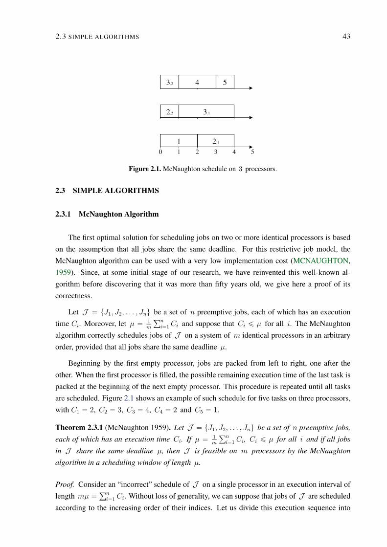
2.3 SIMPLE ALGORITHMS 43
0 1 2 3 4 5
1 2.1
2.2 3.1
3.2 4 5
Figure 2.1. McNaughton schedule on 3 processors.
2.3 SIMPLE ALGORITHMS
2.3.1 McNaughton Algorithm
The first optimal solution for scheduling jobs on two or more identical processors is based
on the assumption that all jobs share the same deadline. For this restrictive job model, the
McNaughton algorithm can be used with a very low implementation cost (MCNAUGHTON,
1959). Since, at some initial stage of our research, we have reinvented this well-known al-
gorithm before discovering that it was more than fifty years old, we give here a proof of its
correctness.
Let J “ tJ1, J2, . . . , Jnu be a set of n preemptive jobs, each of which has an execution
time Ci. Moreover, let µ “ 1
m
řn
i“1Ci and suppose that Ci ď µ for all i. The McNaughton
algorithm correctly schedules jobs of J on a system of m identical processors in an arbitrary
order, provided that all jobs share the same deadline µ.
Beginning by the first empty processor, jobs are packed from left to right, one after the
other. When the first processor is filled, the possible remaining execution time of the last task is
packed at the beginning of the next empty processor. This procedure is repeated until all tasks
are scheduled. Figure 2.1 shows an example of such schedule for five tasks on three processors,
with C1 “ 2, C2 “ 3, C3 “ 4, C4 “ 2 and C5 “ 1.
Theorem 2.3.1 (McNaughton 1959). Let J “ tJ1, J2, . . . , Jnu be a set of n preemptive jobs,
each of which has an execution time Ci. If µ “ 1
m
řn
i“1Ci, Ci ď µ for all i and if all jobs
in J share the same deadline µ, then J is feasible on m processors by the McNaughton
algorithm in a scheduling window of length µ.
Proof. Consider an “incorrect” schedule of J on a single processor in an execution interval of
length mµ “řn
i“1Ci. Without loss of generality, we can suppose that jobs of J are scheduled
according to the increasing order of their indices. Let us divide this execution sequence into
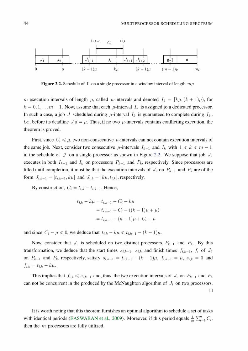
44 MULTIPROCESSOR SCHEDULING SPECTRUM
0 µ pk ´ 1qµ kµ pk ` 1qµ pm´ 1qµ mµ
J1 J2 Ji´1
Citi,k´1 ti,k
Ji Ji`1 Ji`2 n-1 n
Figure 2.2. Schedule of Γ on a single processor in a window interval of length mµ.
m execution intervals of length µ, called µ-intervals and denoted Ik “ rkµ, pk ` 1qµq, for
k “ 0, 1, . . . m ´ 1. Now, assume that each µ-interval Ik is assigned to a dedicated processor.
In such a case, a job J scheduled during µ-interval Ik is guaranteed to complete during Ik ,
i.e., before its deadline J.d “ µ. Thus, if no two µ-intervals contains conflicting execution, the
theorem is proved.
First, since Ci ď µ, two non-consecutive µ-intervals can not contain execution intervals of
the same job. Next, consider two consecutive µ-intervals Ik´1 and Ik with 1 ď k ď m ´ 1
in the schedule of J on a single processor as shown in Figure 2.2. We suppose that job Ji
executes in both Ik´1 and Ik on processors Pk´1 and Pk, respectively. Since processors are
filled until completion, it must be that the execution intervals of Ji on Pk´1 and Pk are of the
form Ji,k´1 “ rti,k´1, kµs and Ji,k “ rkµ, ti,ks, respectively.
By construction, Ci “ ti,k ´ ti,k´1. Hence,
ti,k ´ kµ “ ti,k´1 ` Ci ´ kµ
“ ti,k´1 ` Ci ´ ppk ´ 1qµ ` µq
“ ti,k´1 ´ pk ´ 1qµ ` Ci ´ µ
and since Ci ´ µ ď 0, we deduce that ti,k ´ kµ ď ti,k´1 ´ pk ´ 1qµ.
Now, consider that Ji is scheduled on two distinct processors Pk´1 and Pk. By this
transformation, we deduce that the start times si,k´1, si,k and finish times fi,k´1, fi of Jion Pk´1 and Pk, respectively, satisfy si,k´1 “ ti,k´1 ´ pk ´ 1qµ, fi,k´1 “ µ, si,k “ 0 and
fi,k “ ti,k ´ kµ.
This implies that fi,k ď si,k´1 and, thus, the two execution intervals of Ji on Pk´1 and Pk
can not be concurrent in the produced by the McNaughton algorithm of Ji on two processors.
It is worth noting that this theorem furnishes an optimal algorithm to schedule a set of tasks
with identical periods (EASWARAN et al., 2009). Moreover, if this period equals 1
m
řn
i“1Ci,
then the m processors are fully utilized.
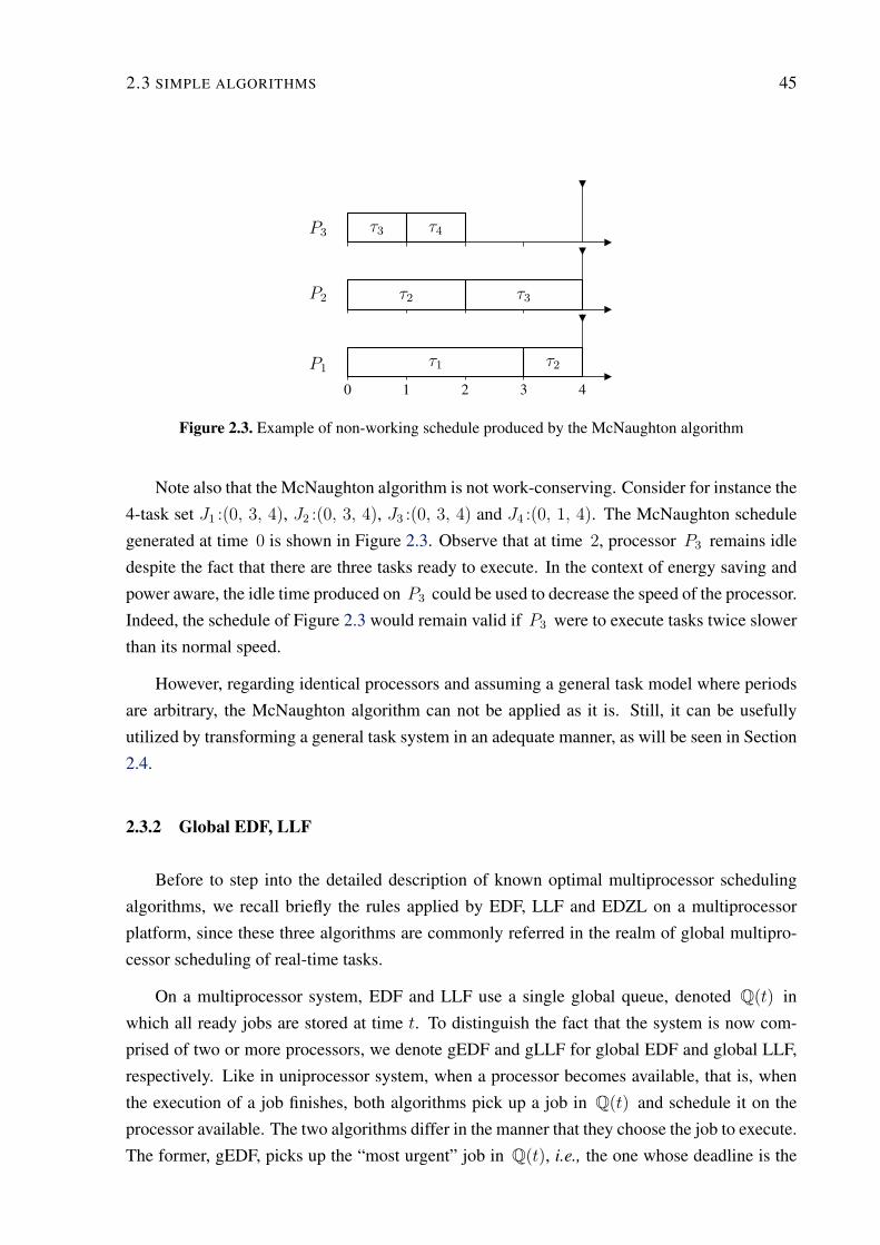
2.3 SIMPLE ALGORITHMS 45
0 1 2 3 4
τ1 τ2
τ2 τ3
τ3 τ4
P1
P2
P3
Figure 2.3. Example of non-working schedule produced by the McNaughton algorithm
Note also that the McNaughton algorithm is not work-conserving. Consider for instance the
4-task set J1 :p0, 3, 4q, J2 :p0, 3, 4q, J3 :p0, 3, 4q and J4 :p0, 1, 4q. The McNaughton schedule
generated at time 0 is shown in Figure 2.3. Observe that at time 2, processor P3 remains idle
despite the fact that there are three tasks ready to execute. In the context of energy saving and
power aware, the idle time produced on P3 could be used to decrease the speed of the processor.
Indeed, the schedule of Figure 2.3 would remain valid if P3 were to execute tasks twice slower
than its normal speed.
However, regarding identical processors and assuming a general task model where periods
are arbitrary, the McNaughton algorithm can not be applied as it is. Still, it can be usefully
utilized by transforming a general task system in an adequate manner, as will be seen in Section
2.4.
2.3.2 Global EDF, LLF
Before to step into the detailed description of known optimal multiprocessor scheduling
algorithms, we recall briefly the rules applied by EDF, LLF and EDZL on a multiprocessor
platform, since these three algorithms are commonly referred in the realm of global multipro-
cessor scheduling of real-time tasks.
On a multiprocessor system, EDF and LLF use a single global queue, denoted Qptq in
which all ready jobs are stored at time t. To distinguish the fact that the system is now com-
prised of two or more processors, we denote gEDF and gLLF for global EDF and global LLF,
respectively. Like in uniprocessor system, when a processor becomes available, that is, when
the execution of a job finishes, both algorithms pick up a job in Qptq and schedule it on the
processor available. The two algorithms differ in the manner that they choose the job to execute.
The former, gEDF, picks up the “most urgent” job in Qptq, i.e., the one whose deadline is the
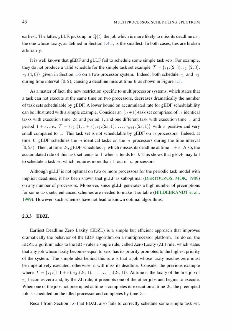
46 MULTIPROCESSOR SCHEDULING SPECTRUM
earliest. The latter, gLLF, picks up in Qptq the job which is more likely to miss its deadline i.e.,
the one whose laxity, as defined in Section 1.4.1, is the smallest. In both cases, ties are broken
arbitrarily.
It is well known that gEDF and gLLF fail to schedule some simple task sets. For example,
they do not produce a valid schedule for the simple task set example T “ tτ1 :p2, 3q, τ2 :p2, 3q,
τ3 :p4, 6qu given in Section 1.6 on a two-processor system. Indeed, both schedule τ1 and τ2
during time interval r0, 2q, causing a deadline miss at time 6 as shown in Figure 1.3.
As a matter of fact, the new restriction specific to multiprocessor systems, which states that
a task can not execute at the same time on two processors, decreases dramatically the number
of task sets schedulable by gEDF. A lower bound on accumulated rate for gEDF schedulability
can be illustrated with a simple example. Consider an pn`1q-task set comprised of n identical
tasks with execution time 2ε and period 1, and one different task with execution time 1 and
period 1 ` ε; i.e., T “ tτ1 :p1, 1 ` εq, τ2 :p2ε, 1q, . . . , τn`1 :p2ε, 1qu with ε positive and very
small compared to 1. This task set is not schedulable by gEDF on n processors. Indeed, at
time 0, gEDF schedules the n identical tasks on the n processors during the time interval
r0, 2εq. Then, at time 2ε, gEDF schedules τ1 which misses its deadline at time 1` ε. Also, the
accumulated rate of this task set tends to 1 when ε tends to 0. This shows that gEDF may fail
to schedule a task set which requires more than 1 out of n processors.
Although gLLF is not optimal on two or more processors for the periodic task model with
implicit deadlines, it has been shown that gLLF is suboptimal (DERTOUZOS; MOK, 1989)
on any number of processors. Moreover, since gLLF generates a high number of preemptions
for some task sets, enhanced schemes are needed to make it suitable (HILDEBRANDT et al.,
1999). However, such schemes have not lead to known optimal algorithms.
2.3.3 EDZL
Earliest Deadline Zero Laxity (EDZL) is a simple but efficient approach that improves
dramatically the behavior of the EDF algorithm on a multiprocessor platform. To do so, the
EDZL algorithm adds to the EDF rules a single rule, called Zero Laxity (ZL) rule, which states
that any job whose laxity becomes equal to zero has its priority promoted to the highest priority
of the system. The simple idea behind this rule is that a job whose laxity reaches zero must
be imperatively executed, otherwise, it will miss its deadline. Consider the previous example
where T “ tτ1 :p1, 1 ` εq, τ2 :p2ε, 1q, . . . , τn`1 :p2ε, 1qu. At time ε, the laxity of the first job of
τ1 becomes zero and, by the ZL rule, it preempts one of the other jobs and begins to execute.
When one of the jobs not preempted at time ε completes its execution at time 2ε, the preempted
job is scheduled on the idled processor and completes by time 3ε.
Recall from Section 1.6 that EDZL also fails to correctly schedule some simple task set.
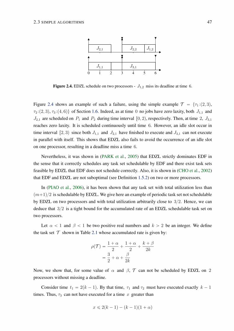
2.3 SIMPLE ALGORITHMS 47
0 1 2 3 4 5 6
J1,1
J2,1 J1,2J2,2
J3,1
Figure 2.4. EDZL schedule on two processors - J1,2 miss its deadline at time 6.
Figure 2.4 shows an example of such a failure, using the simple example T “ tτ1 :p2, 3q,
τ2 :p2, 3q, τ3 :p4, 6qu of Section 1.6. Indeed, as at time 0 no jobs have zero laxity, both J1,1 and
J2,1 are scheduled on P1 and P2 during time interval r0, 2q, respectively. Then, at time 2, J3,1reaches zero laxity. It is scheduled continuously until time 6. However, an idle slot occur in
time interval r2, 3q since both J1,1 and J2,1 have finished to execute and J3,1 can not execute
in parallel with itself. This shows that EDZL also fails to avoid the occurrence of an idle slot
on one processor, resulting in a deadline miss a time 6.
Nevertheless, it was shown in (PARK et al., 2005) that EDZL strictly dominates EDF in
the sense that it correctly schedules any task set schedulable by EDF and there exist task sets
feasible by EDZL that EDF does not schedule correctly. Also, it is shown in (CHO et al., 2002)
that EDF and EDZL are not suboptimal (see Definition 1.5.2) on two or more processors.
In (PIAO et al., 2006), it has been shown that any task set with total utilization less than
pm`1q2 is schedulable by EDZL. We give here an example of periodic task set not schedulable
by EDZL on two processors and with total utilization arbitrarily close to 32. Hence, we can
deduce that 32 is a tight bound for the accumulated rate of an EDZL schedulable task set on
two processors.
Let α ă 1 and β ă 1 be two positive real numbers and k ą 2 be an integer. We define
the task set T shown in Table 2.1 whose accumulated rate is given by:
ρpT q “1 ` α
2`
1 ` α
2`k ` β
2k
“3
2` α `
β
2k
Now, we show that, for some value of α and β, T can not be scheduled by EDZL on 2
processors without missing a deadline.
Consider time t1 “ 2pk ´ 1q. By that time, τ1 and τ2 must have executed exactly k ´ 1
times. Thus, τ3 can not have executed for a time x greater than
x ď 2pk ´ 1q ´ pk ´ 1qp1 ` αq
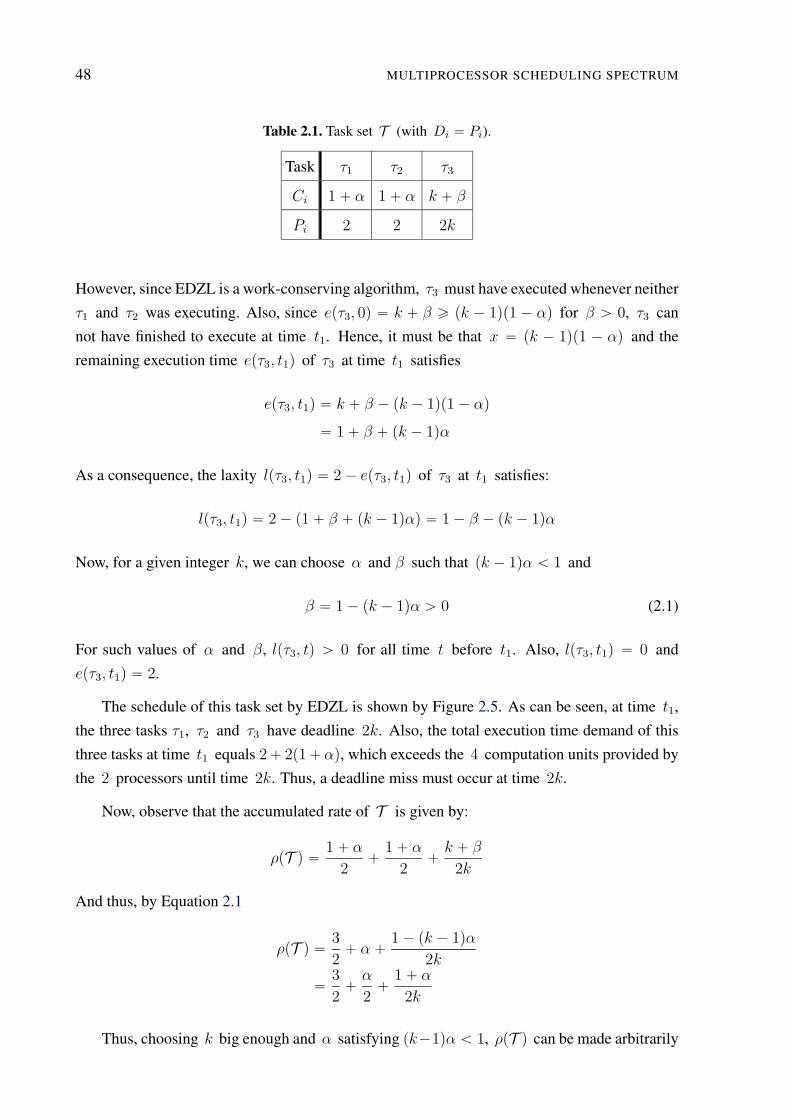
48 MULTIPROCESSOR SCHEDULING SPECTRUM
Table 2.1. Task set T (with Di “ Pi).
Task τ1 τ2 τ3
Ci 1 ` α 1 ` α k ` β
Pi 2 2 2k
However, since EDZL is a work-conserving algorithm, τ3 must have executed whenever neither
τ1 and τ2 was executing. Also, since epτ3, 0q “ k ` β ě pk ´ 1qp1 ´ αq for β ą 0, τ3 can
not have finished to execute at time t1. Hence, it must be that x “ pk ´ 1qp1 ´ αq and the
remaining execution time epτ3, t1q of τ3 at time t1 satisfies
epτ3, t1q “ k ` β ´ pk ´ 1qp1 ´ αq
“ 1 ` β ` pk ´ 1qα
As a consequence, the laxity lpτ3, t1q “ 2 ´ epτ3, t1q of τ3 at t1 satisfies:
lpτ3, t1q “ 2 ´ p1 ` β ` pk ´ 1qαq “ 1 ´ β ´ pk ´ 1qα
Now, for a given integer k, we can choose α and β such that pk ´ 1qα ă 1 and
β “ 1 ´ pk ´ 1qα ą 0 (2.1)
For such values of α and β, lpτ3, tq ą 0 for all time t before t1. Also, lpτ3, t1q “ 0 and
epτ3, t1q “ 2.
The schedule of this task set by EDZL is shown by Figure 2.5. As can be seen, at time t1,
the three tasks τ1, τ2 and τ3 have deadline 2k. Also, the total execution time demand of this
three tasks at time t1 equals 2` 2p1`αq, which exceeds the 4 computation units provided by
the 2 processors until time 2k. Thus, a deadline miss must occur at time 2k.
Now, observe that the accumulated rate of T is given by:
ρpT q “1 ` α
2`
1 ` α
2`k ` β
2k
And thus, by Equation 2.1
ρpT q “3
2` α `
1 ´ pk ´ 1qα
2k
“3
2`α
2`
1 ` α
2k
Thus, choosing k big enough and α satisfying pk´1qα ă 1, ρpT q can be made arbitrarily
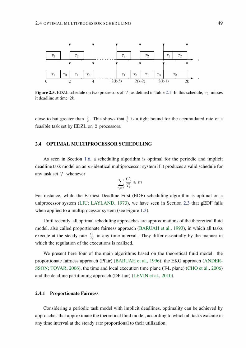
2.4 OPTIMAL MULTIPROCESSOR SCHEDULING 49
0 2 4 2(k-3) 2(k-2) 2(k-1) 2k
τ1
τ2
τ3 τ1
τ2
τ3 τ1
τ2
τ3 τ1
τ2
τ3
τ1 τ2
τ3
Figure 2.5. EDZL schedule on two processors of T as defined in Table 2.1. In this schedule, τ1 missesit deadline at time 2k.
close to but greater than 3
2. This shows that 3
2is a tight bound for the accumulated rate of a
feasible task set by EDZL on 2 processors.
2.4 OPTIMAL MULTIPROCESSOR SCHEDULING
As seen in Section 1.6, a scheduling algorithm is optimal for the periodic and implicit
deadline task model on an m-identical multiprocessor system if it produces a valid schedule for
any task set T wheneverÿ
τiPT
Ci
Tiď m
For instance, while the Earliest Deadline First (EDF) scheduling algorithm is optimal on a
uniprocessor system (LIU; LAYLAND, 1973), we have seen in Section 2.3 that gEDF fails
when applied to a multiprocessor system (see Figure 1.3).
Until recently, all optimal scheduling approaches are approximations of the theoretical fluid
model, also called proportionate fairness approach (BARUAH et al., 1993), in which all tasks
execute at the steady rate Ci
Tiin any time interval. They differ essentially by the manner in
which the regulation of the executions is realized.
We present here four of the main algorithms based on the theoretical fluid model: the
proportionate fairness approach (Pfair) (BARUAH et al., 1996), the EKG approach (ANDER-
SSON; TOVAR, 2006), the time and local execution time plane (T-L plane) (CHO et al., 2006)
and the deadline partitioning approach (DP-fair) (LEVIN et al., 2010).
2.4.1 Proportionate Fairness
Considering a periodic task model with implicit deadlines, optimality can be achieved by
approaches that approximate the theoretical fluid model, according to which all tasks execute in
any time interval at the steady rate proportional to their utilization.
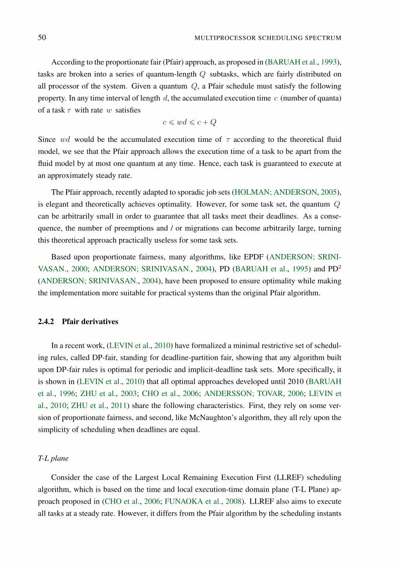
50 MULTIPROCESSOR SCHEDULING SPECTRUM
According to the proportionate fair (Pfair) approach, as proposed in (BARUAH et al., 1993),
tasks are broken into a series of quantum-length Q subtasks, which are fairly distributed on
all processor of the system. Given a quantum Q, a Pfair schedule must satisfy the following
property. In any time interval of length d, the accumulated execution time c (number of quanta)
of a task τ with rate w satisfies
c ď wd ď c ` Q
Since wd would be the accumulated execution time of τ according to the theoretical fluid
model, we see that the Pfair approach allows the execution time of a task to be apart from the
fluid model by at most one quantum at any time. Hence, each task is guaranteed to execute at
an approximately steady rate.
The Pfair approach, recently adapted to sporadic job sets (HOLMAN; ANDERSON, 2005),
is elegant and theoretically achieves optimality. However, for some task set, the quantum Q
can be arbitrarily small in order to guarantee that all tasks meet their deadlines. As a conse-
quence, the number of preemptions and / or migrations can become arbitrarily large, turning
this theoretical approach practically useless for some task sets.
Based upon proportionate fairness, many algorithms, like EPDF (ANDERSON; SRINI-
VASAN., 2000; ANDERSON; SRINIVASAN., 2004), PD (BARUAH et al., 1995) and PD2
(ANDERSON; SRINIVASAN., 2004), have been proposed to ensure optimality while making
the implementation more suitable for practical systems than the original Pfair algorithm.
2.4.2 Pfair derivatives
In a recent work, (LEVIN et al., 2010) have formalized a minimal restrictive set of schedul-
ing rules, called DP-fair, standing for deadline-partition fair, showing that any algorithm built
upon DP-fair rules is optimal for periodic and implicit-deadline task sets. More specifically, it
is shown in (LEVIN et al., 2010) that all optimal approaches developed until 2010 (BARUAH
et al., 1996; ZHU et al., 2003; CHO et al., 2006; ANDERSSON; TOVAR, 2006; LEVIN et
al., 2010; ZHU et al., 2011) share the following characteristics. First, they rely on some ver-
sion of proportionate fairness, and second, like McNaughton’s algorithm, they all rely upon the
simplicity of scheduling when deadlines are equal.
T-L plane
Consider the case of the Largest Local Remaining Execution First (LLREF) scheduling
algorithm, which is based on the time and local execution-time domain plane (T-L Plane) ap-
proach proposed in (CHO et al., 2006; FUNAOKA et al., 2008). LLREF also aims to execute
all tasks at a steady rate. However, it differs from the Pfair algorithm by the scheduling instants
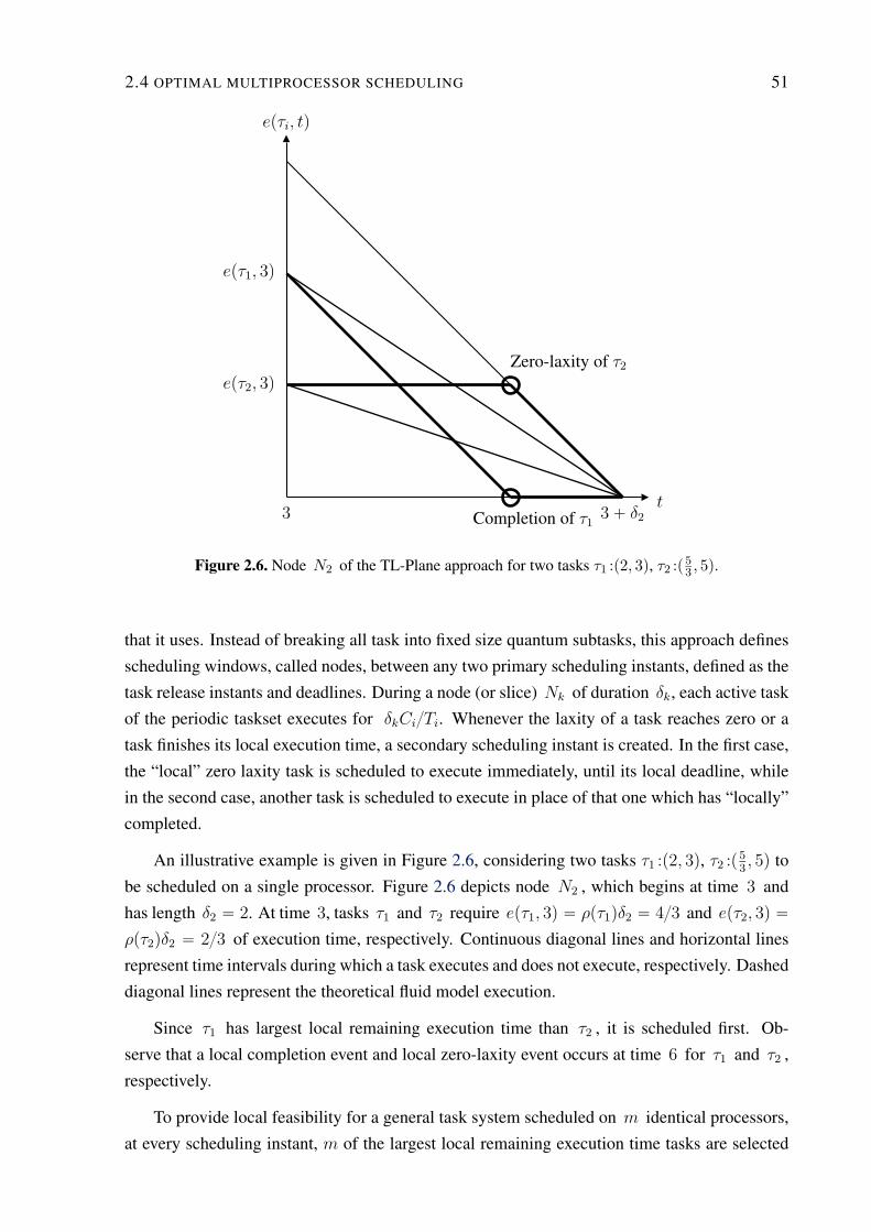
2.4 OPTIMAL MULTIPROCESSOR SCHEDULING 51
epτi, tq
t3 3 ` δ2
epτ1, 3q
epτ2, 3qZero-laxity of τ2
Completion of τ1
Figure 2.6. Node N2 of the TL-Plane approach for two tasks τ1 :p2, 3q, τ2 :p53 , 5q.
that it uses. Instead of breaking all task into fixed size quantum subtasks, this approach defines
scheduling windows, called nodes, between any two primary scheduling instants, defined as the
task release instants and deadlines. During a node (or slice) Nk of duration δk, each active task
of the periodic taskset executes for δkCiTi. Whenever the laxity of a task reaches zero or a
task finishes its local execution time, a secondary scheduling instant is created. In the first case,
the “local” zero laxity task is scheduled to execute immediately, until its local deadline, while
in the second case, another task is scheduled to execute in place of that one which has “locally”
completed.
An illustrative example is given in Figure 2.6, considering two tasks τ1 :p2, 3q, τ2 :p5
3, 5q to
be scheduled on a single processor. Figure 2.6 depicts node N2 , which begins at time 3 and
has length δ2 “ 2. At time 3, tasks τ1 and τ2 require epτ1, 3q “ ρpτ1qδ2 “ 43 and epτ2, 3q “
ρpτ2qδ2 “ 23 of execution time, respectively. Continuous diagonal lines and horizontal lines
represent time intervals during which a task executes and does not execute, respectively. Dashed
diagonal lines represent the theoretical fluid model execution.
Since τ1 has largest local remaining execution time than τ2 , it is scheduled first. Ob-
serve that a local completion event and local zero-laxity event occurs at time 6 for τ1 and τ2 ,
respectively.
To provide local feasibility for a general task system scheduled on m identical processors,
at every scheduling instant, m of the largest local remaining execution time tasks are selected
52 MULTIPROCESSOR SCHEDULING SPECTRUM
0 1 2 3 4 5 6 7 8 9 10 11 12 13 14 15
τ1 τ2
τ3
τ3
τ4 τ5
τ1 τ2 τ3
τ3 τ4 τ5
τ1 τ2 τ3
τ3 τ4 τ5
τ1 τ2 τ3
τ3 τ4 τ5
τ1 τ2 τ3
τ3 τ4 τ5
Figure 2.7. DP-wrap schedule of task set T “ tτ1 :p2, 5q, τ2 :p3.2, 8q, τ3 :p4, 10q,τ4 :p4.8, 12q, τ5 :p6, 15qu
first, hence the name LLREF of the scheduling policy.
In (FUNK, 2010), the T-L plane approach is extended to the sporadic task model with
unconstrained deadlines.
DP-wrap
As an example of a simple optimal algorithm built upon DP-fair rules, the DP-wrap schedul-
ing algorithm is proposed in (LEVIN et al., 2010). Similarly to T-L plane, time is divided into
time slices, i.e., the nodes in the T-L plane approach, of length equal to the distance between two
distinct and consecutive deadlines in the system. During a time slice k, each task τi executes
for its local execution time which is proportional to the rate of τi and the duration δk of slice k.
Precisely, if Ci,k is the local execution time of task τi during slice k, then
Ci,k “ ρpτiqδk
Doing so, the original problem is transformed into an easier problem in each slice since all
pieces of jobs in a slice share the same (slice) deadline. Differently from the T-L plane ap-
proach, this easier problem is then solved using the McNaughton algorithm (MCNAUGHTON,
1959), previously described in Section 2.3. Since the McNaughton algorithm is optimal when
deadlines of tasks are equal, the DP-wrap implementation of the DP-fair rules is optimal.
We illustrate the DP-wrap algorithm with the simple task set T “ tτ1 :p2, 5q, τ2 :p3.2, 8q,
τ3 :p4, 10q, τ4 :p4.8, 12q, τ5 :p6, 15qu . The corresponding DP-wrap schedule is shown in Figure
2.7.
EKG
The EKG approach, as a short-hand notation for EDF with task splitting and k processors
in a group, has been proposed in (ANDERSSON; TOVAR, 2006), a couple of years before
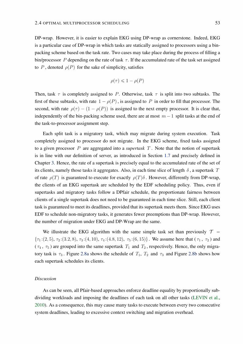
2.4 OPTIMAL MULTIPROCESSOR SCHEDULING 53
DP-wrap. However, it is easier to explain EKG using DP-wrap as cornerstone. Indeed, EKG
is a particular case of DP-wrap in which tasks are statically assigned to processors using a bin-
packing scheme based on the task rate. Two cases may take place during the process of filling a
bin/processor P depending on the rate of task τ . If the accumulated rate of the task set assigned
to P , denoted ρpP q for the sake of simplicity, satisfies
ρpτq ď 1 ´ ρpP q
Then, task τ is completely assigned to P . Otherwise, task τ is split into two subtasks. The
first of these subtasks, with rate 1 ´ ρpP q , is assigned to P in order to fill that processor. The
second, with rate ρpτq ´ p1 ´ ρpP qq is assigned to the next empty processor. It is clear that,
independently of the bin-packing scheme used, there are at most m´ 1 split tasks at the end of
the task-to-processor assignment step.
Each split task is a migratory task, which may migrate during system execution. Task
completely assigned to processor do not migrate. In the EKG scheme, fixed tasks assigned
to a given processor P are aggregated into a supertask T . Note that the notion of supertask
is in line with our definition of server, as introduced in Section 1.7 and precisely defined in
Chapter 3. Hence, the rate of a supertask is precisely equal to the accumulated rate of the set of
its clients, namely those tasks it aggregates. Also, in each time slice of length δ , a supertask T
of rate ρpT q is guaranteed to execute for exactly ρpT qδ . However, differently from DP-wrap,
the clients of an EKG supertask are scheduled by the EDF scheduling policy. Thus, even if
supertasks and migratory tasks follow a DPfair schedule, the proportionate fairness between
clients of a single supertask does not need to be guaranteed in each time slice. Still, each client
task is guaranteed to meet its deadlines, provided that its supertask meets them. Since EKG uses
EDF to schedule non-migratory tasks, it generates fewer preemptions than DP-wrap. However,
the number of migration under EKG and DP-Wrap are the same.
We illustrate the EKG algorithm with the same simple task set than previously T “
tτ1 :p2, 5q, τ2 :p3.2, 8q, τ3 :p4, 10q, τ4 :p4.8, 12q, τ5 :p6, 15qu . We assume here that ( τ1 , τ2 ) and
( τ4 , τ5 ) are grouped into the same supertask T1 and T2 , respectively. Hence, the only migra-
tory task is τ3 . Figure 2.8a shows the schedule of T1, T2 and τ3 and Figure 2.8b shows how
each supertask schedules its clients.
Discussion
As can be seen, all Pfair-based approaches enforce deadline equality by proportionally sub-
dividing workloads and imposing the deadlines of each task on all other tasks (LEVIN et al.,
2010). As a consequence, this may cause many tasks to execute between every two consecutive
system deadlines, leading to excessive context switching and migration overhead.
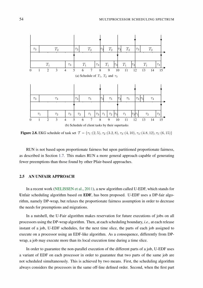
54 MULTIPROCESSOR SCHEDULING SPECTRUM
0 1 2 3 4 5 6 7 8 9 10 11 12 13 14 15
T1
τ3
τ3
T2
T1 τ3
τ3 T2
T1 τ3
τ3 T2
T1 τ3
τ3 T2
T1 τ3
τ3 T2
(a) Schedule of T1, T2 and τ3
0 1 2 3 4 5 6 7 8 9 10 11 12 13 14 15
τ1 τ2
τ3
τ3
τ4
τ2 τ1 τ3
τ3 τ5
τ1 τ2 τ3
τ3 τ5
τ1 τ3
τ3 τ5
τ1 τ2 τ3
τ3 τ5 τ4
(b) Schedule of client tasks by their supertasks
Figure 2.8. EKG schedule of task set T “ tτ1 :p2, 5q, τ2 :p3.2, 8q, τ3 :p4, 10q, τ4 :p4.8, 12q, τ5 :p6, 15qu
RUN is not based upon proportionate fairness but upon partitioned proportionate fairness,
as described in Section 1.7. This makes RUN a more general approach capable of generating
fewer preemptions than those found by other Pfair-based approaches.
2.5 AN UNFAIR APPROACH
In a recent work (NELISSEN et al., 2011), a new algorithm called U-EDF, which stands for
Unfair scheduling algorithm based on EDF, has been proposed. U-EDF uses a DP-fair algo-
rithm, namely DP-wrap, but relaxes the proportionate fairness assumption in order to decrease
the needs for preemptions and migrations.
In a nutshell, the U-Fair algorithm makes reservation for future executions of jobs on all
processors using the DP-wrap algorithm. Then, at each scheduling boundary, i.e., at each release
instant of a job, U-EDF schedules, for the next time slice, the parts of each job assigned to
execute on a processor using an EDF-like algorithm. As a consequence, differently from DP-
wrap, a job may execute more than its local execution time during a time slice.
In order to guarantee the non-parallel execution of the different parts of a job, U-EDF uses
a variant of EDF on each processor in order to guarantee that two parts of the same job are
not scheduled simultaneously. This is achieved by two means. First, the scheduling algorithm
always considers the processors in the same off-line defined order. Second, when the first part
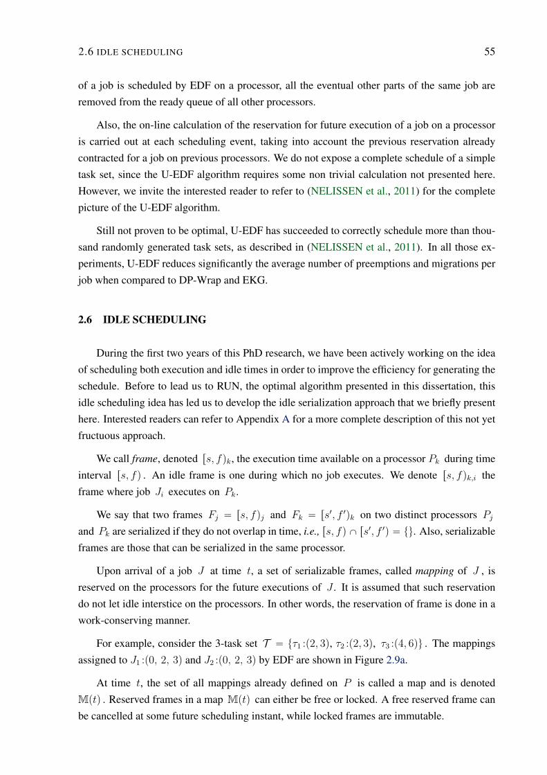
2.6 IDLE SCHEDULING 55
of a job is scheduled by EDF on a processor, all the eventual other parts of the same job are
removed from the ready queue of all other processors.
Also, the on-line calculation of the reservation for future execution of a job on a processor
is carried out at each scheduling event, taking into account the previous reservation already
contracted for a job on previous processors. We do not expose a complete schedule of a simple
task set, since the U-EDF algorithm requires some non trivial calculation not presented here.
However, we invite the interested reader to refer to (NELISSEN et al., 2011) for the complete
picture of the U-EDF algorithm.
Still not proven to be optimal, U-EDF has succeeded to correctly schedule more than thou-
sand randomly generated task sets, as described in (NELISSEN et al., 2011). In all those ex-
periments, U-EDF reduces significantly the average number of preemptions and migrations per
job when compared to DP-Wrap and EKG.
2.6 IDLE SCHEDULING
During the first two years of this PhD research, we have been actively working on the idea
of scheduling both execution and idle times in order to improve the efficiency for generating the
schedule. Before to lead us to RUN, the optimal algorithm presented in this dissertation, this
idle scheduling idea has led us to develop the idle serialization approach that we briefly present
here. Interested readers can refer to Appendix A for a more complete description of this not yet
fructuous approach.
We call frame, denoted rs, fqk, the execution time available on a processor Pk during time
interval rs, fq . An idle frame is one during which no job executes. We denote rs, fqk,i the
frame where job Ji executes on Pk.
We say that two frames Fj “ rs, fqj and Fk “ rs1, f 1qk on two distinct processors Pj
and Pk are serialized if they do not overlap in time, i.e., rs, fq X rs1, f 1q “ tu. Also, serializable
frames are those that can be serialized in the same processor.
Upon arrival of a job J at time t, a set of serializable frames, called mapping of J , is
reserved on the processors for the future executions of J . It is assumed that such reservation
do not let idle interstice on the processors. In other words, the reservation of frame is done in a
work-conserving manner.
For example, consider the 3-task set T “ tτ1 :p2, 3q, τ2 :p2, 3q, τ3 :p4, 6qu . The mappings
assigned to J1 :p0, 2, 3q and J2 :p0, 2, 3q by EDF are shown in Figure 2.9a.
At time t, the set of all mappings already defined on P is called a map and is denoted
Mptq . Reserved frames in a map Mptq can either be free or locked. A free reserved frame can
be cancelled at some future scheduling instant, while locked frames are immutable.
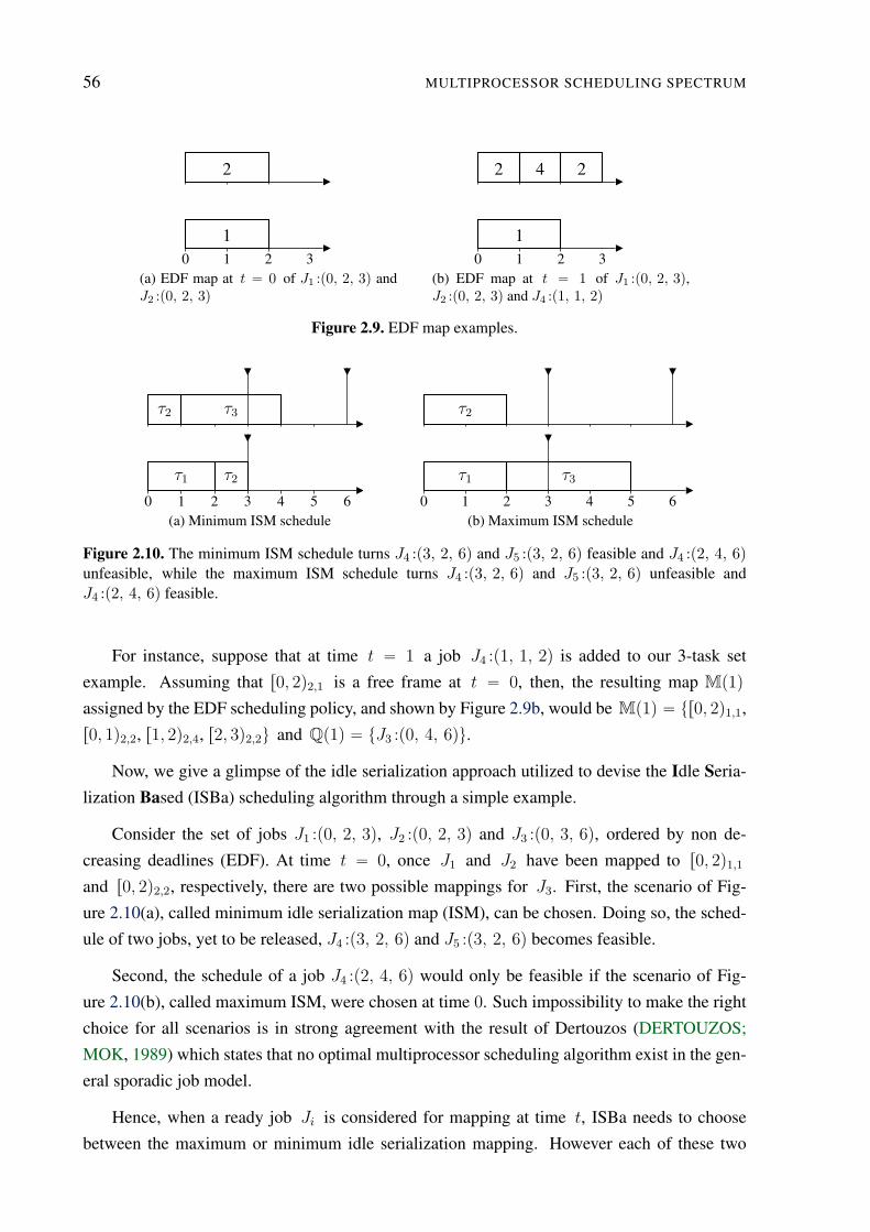
56 MULTIPROCESSOR SCHEDULING SPECTRUM
0 1 2 3
1
2
(a) EDF map at t “ 0 of J1 :p0, 2, 3q andJ2 :p0, 2, 3q
0 1 2 3
1
2 4 2
(b) EDF map at t “ 1 of J1 :p0, 2, 3q,J2 :p0, 2, 3q and J4 :p1, 1, 2q
Figure 2.9. EDF map examples.
0 1 2 3 4 5 6
τ1 τ2
τ2 τ3
(a) Minimum ISM schedule0 1 2 3 4 5 6
τ1
τ2
τ3
(b) Maximum ISM schedule
Figure 2.10. The minimum ISM schedule turns J4 :p3, 2, 6q and J5 :p3, 2, 6q feasible and J4 :p2, 4, 6qunfeasible, while the maximum ISM schedule turns J4 :p3, 2, 6q and J5 :p3, 2, 6q unfeasible andJ4 :p2, 4, 6q feasible.
For instance, suppose that at time t “ 1 a job J4 :p1, 1, 2q is added to our 3-task set
example. Assuming that r0, 2q2,1 is a free frame at t “ 0, then, the resulting map Mp1q
assigned by the EDF scheduling policy, and shown by Figure 2.9b, would be Mp1q “ tr0, 2q1,1,
r0, 1q2,2, r1, 2q2,4, r2, 3q2,2u and Qp1q “ tJ3 :p0, 4, 6qu.
Now, we give a glimpse of the idle serialization approach utilized to devise the Idle Seria-
lization Based (ISBa) scheduling algorithm through a simple example.
Consider the set of jobs J1 :p0, 2, 3q, J2 :p0, 2, 3q and J3 :p0, 3, 6q, ordered by non de-
creasing deadlines (EDF). At time t “ 0, once J1 and J2 have been mapped to r0, 2q1,1
and r0, 2q2,2, respectively, there are two possible mappings for J3. First, the scenario of Fig-
ure 2.10(a), called minimum idle serialization map (ISM), can be chosen. Doing so, the sched-
ule of two jobs, yet to be released, J4 :p3, 2, 6q and J5 :p3, 2, 6q becomes feasible.
Second, the schedule of a job J4 :p2, 4, 6q would only be feasible if the scenario of Fig-
ure 2.10(b), called maximum ISM, were chosen at time 0. Such impossibility to make the right
choice for all scenarios is in strong agreement with the result of Dertouzos (DERTOUZOS;
MOK, 1989) which states that no optimal multiprocessor scheduling algorithm exist in the gen-
eral sporadic job model.
Hence, when a ready job Ji is considered for mapping at time t, ISBa needs to choose
between the maximum or minimum idle serialization mapping. However each of these two
2.7 CONCLUSION 57
choices has consequences. Choosing the maximum ISM scenario may turn feasible a ready job,
taking advantage of the full length of the longest idle time. On the other hand, choosing the
minimum ISM may turn feasible two jobs with low laxity, yet to be released.
As a consequence, we adopted the following scheduling rules for the ISBa algorithm. While
no ready jobs can execute, thanks to the idle serialization, ISBa chooses the minimum idle
serialization schedule. Otherwise, ISBa opts for the maximum idle serialization schedule. In
other words, ISBa only chooses a maximum ISM schedule when this choice does not cause the
idling of a processor. Otherwise, ISBa chooses the minimum ISM schedule.
2.6.1 Discussion
We have successfully implemented the ISBa algorithm. However, after more than a year
of intensive work, we were disappointed because ISBa was only capable to schedule about
the same number of fully-utilization task sets as EDZL when using random task set generated
by the open-source random task generator developed by Emberson (EMBERSON et al., 2010;
EMBERSON et al., 2011). Since the ISBa implementation was much more complicated than
that of EDZL, we concluded that, in general, the idle serialization approach was not worth it
from an implementation viewpoint.
Nevertheless, the idea of scheduling the idle time of a task instead of its execution time
remained as a promising cornerstone from this unsuccessful serialization approach. A couple
of months latter, this idea gave birth to our reduction to uniprocessor algorithm, which is partly
based upon duality, i.e., idle scheduling.
Other related work may be found on the topics of duality. For instance, a recent and not
yet published work (LEVIN et al., 2009) establishes that if a set T of m ` 1 tasks have their
total utilization exactly equal to m, then a dual-based algorithm produces a feasible schedule
of these tasks on m processors. This result can be seen as a special case of the approach being
proposed here.
2.7 CONCLUSION
Up to date, optimality in multiprocessor scheduling has mainly been achieved through dif-
ferent variations of the proportionate fairness (Pfair) idea as proposed in (BARUAH et al.,
1993). It is only recently that a new approach U-EDF, based on a DP-fair algorithm, but re-
laxing the fairness constraint has been proposed in (NELISSEN et al., 2011). Although not
proved to achieve optimality for periodic task systems with implicit deadlines, the relaxation
of the fairness constraint allows U-EDF for achieving much lower preemption overhead than
previous Pfair-based algorithms.
58 MULTIPROCESSOR SCHEDULING SPECTRUM
As will be exposed in the remaining chapters of this dissertation, the RUN algorithm, first
published in (REGNIER et al., 2011), also achieves a low preemption overhead by relaxing
the fairness constraint through the clever use of servers to aggregate low rate tasks. Also, the
combination of such servers with the idle scheduling idea leads to the original reduction to
uniprocessor approach exposed in this dissertation, the first to our knowledge, not based on
Pfair and proven to be optimal for periodic task systems with implicit deadlines.
Chapter
3The reduction of the number of task of a general task system is obtained by aggregating many low rate tasks
compared to one into single servers of accumulated rate less than or equal to one. Since a server can schedule its
clients on a single processor, we establish the properties of servers simply considering a uniprocessor system.
TASKS AND SERVERS
3.1 INTRODUCTION
As briefly mentioned in Section 1.7 of Chapter 1, the partitioned proportionate fairness (PP-
Fair) approach relies on the aggregation of low rate tasks, the clients, into virtual scheduling
entities, the servers, such that each server has high, but less than one, accumulated rate.
For instance, in the first off-line step of the Reduction to Uniprocessor (RUN) scheduling
procedure, a set of servers is defined such that each primal task is associated to a unique primal
server. Regarding this primal system of servers, RUN is partitioned proportionate fair in the
sense that each server is guaranteed to execute at a fixed rate, equal to the sum of its clients’
rates, between any two of its clients’ deadlines.
Since tasks and servers play a central role in the RUN algorithm, we dedicated this chapter
to their precise definition and to the description of their properties.
Note that the concept of task servers has been extensively used to provide a mechanism to
schedule soft real-time tasks (LIU, 2000), for which timing attributes like period or execution
time are not known a priori. There are server mechanisms for uniprocessor systems which share
some similarities with the one presented here (DENG et al., 1997; SPURI; BUTTAZZO, 1996).
Other server mechanisms have been designed for multiprocessor systems, e.g., (MOIR; RA-
MAMURTHY, 1999; ANDERSSON; TOVAR, 2006; ANDERSSON et al., 2008). However,
unlike such approaches, the mechanism described here works as if each server were a unipro-
cessor system providing a useful scheduling framework which hides some complexities related
to the multiprocessor scheduling problem.
59
60 TASKS AND SERVERS
Structure of the chapter
In Section 3.2, we introduce a slightly more general specification for a real-time task than
the usual periodic-preemptive and independent with implicit deadlines (PPID) task model.
Then, we present the fully-utilization system assumption adopted in this dissertation in Sec-
tion 3.3, before to step into the full description of a server and its properties in Section 3.4. The
Chapter finishes with a discussion of partial knowledge in Section 3.5 and partitioned propor-
tionate fairness in Section 3.6.
3.2 FIXED-RATE TASK MODEL
Recall from Section 1.2.1 that a real-time job J is a finite sequence of instructions to be
executed on one or more processors with a release instant J.r, a worst-case execution time J.c
and a deadline J.d.
In order to represent possibly non-periodic execution requirements, like those of servers
in particular, we introduce a general real-time object, called fixed-rate task, whose execution
requirement is specified in terms of processor utilization within a given interval. Since a task
shall be able to execute on a single processor, its utilization cannot be greater than one. Although
the definition of a fixed-rate task is slightly different from the usual definition of real-time task
as given in Section 1.2.2, we somehow abusively will simply call task a fixed-rate task when no
confusion is introduced doing so in the remaining of this dissertation.
Definition 3.2.1 (Fixed-Rate Task). Let ρ ď 1 be a positive real number and K a countable
and unbounded set of positive real numbers, possibly including zero. The fixed-rate task τ
with rate ρ and release instants K, denoted τ :rρ,Ks, releases an infinite sequence of jobs
satisfying the following properties:
i) A job J of τ is released at time t if and only if t is in K;
ii) The deadline J.d of job J released at time J.r equals minttt P K, t ą J.ru;
iii) The execution time J.c of job J released at time J.r equals ρpJ.d ´ J.rq.
As can be seen from point (ii) of this definition, we assume an implicit deadline model,
i.e., the deadline of τ ’s job is precisely equal to the release instant of the next job of τ . As a
consequence, KztminpKqu is also the set of all deadlines of jobs of task τ .
Given a fixed-rate task τ , we denote ρpτq its rate and Rpτq the set of the release instants
of its jobs.
As a simple example of task, consider a periodic task τ characterized by three attributes:
(i) its start time s; (ii) its period T ; and (iii) its execution requirement C. Task τ generates
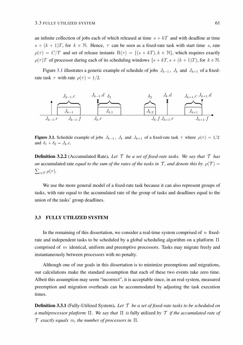
3.3 FULLY UTILIZED SYSTEM 61
an infinite collection of jobs each of which released at time s ` kT and with deadline at time
s ` pk ` 1qT , for k P N. Hence, τ can be seen as a fixed-rate task with start time s, rate
ρpτq “ CT and set of release instants Rpτq “ tps ` kT q, k P Nu, which requires exactly
ρpτqT of processor during each of its scheduling windows rs` kT, s` pk ` 1qT q, for k P N.
Figure 3.1 illustrates a generic example of schedule of jobs Jk´1 , Jk and Jk`1 of a fixed-
rate task τ with rate ρpτq “ 12.
Jk´1.r
Jk´1
Jk´1.c
Jk´1.f
Jk´1.d
Jk.r
Jk,1
δ1
Jk,2
δ2 Jk.d
Jk.f Jk`1.r
Jk`1
Jk`1.c
Jk`1.f
Jk`1.d
Figure 3.1. Schedule example of jobs Jk´1 , Jk and Jk`1 of a fixed-rate task τ where ρpτq “ 12and δ1 ` δ2 “ Jk.c.
Definition 3.2.2 (Accumulated Rate). Let T be a set of fixed-rate tasks. We say that T has
an accumulated rate equal to the sum of the rates of the tasks in T , and denote this by ρpT q “ř
τPT ρpτq.
We use the more general model of a fixed-rate task because it can also represent groups of
tasks, with rate equal to the accumulated rate of the group of tasks and deadlines equal to the
union of the tasks’ group deadlines.
3.3 FULLY UTILIZED SYSTEM
In the remaining of this dissertation, we consider a real-time system comprised of n fixed-
rate and independent tasks to be scheduled by a global scheduling algorithm on a platform Π
comprised of m identical, uniform and preemptive processors. Tasks may migrate freely and
instantaneously between processors with no penalty.
Although one of our goals in this dissertation is to minimize preemptions and migrations,
our calculations make the standard assumption that each of these two events take zero time.
Albeit this assumption may seem “incorrect”, it is acceptable since, in an real system, measured
preemption and migration overheads can be accommodated by adjusting the task execution
times.
Definition 3.3.1 (Fully-Utilized System). Let T be a set of fixed-rate tasks to be scheduled on
a multiprocessor platform Π . We say that Π is fully utilized by T if the accumulated rate of
T exactly equals m, the number of processors in Π.
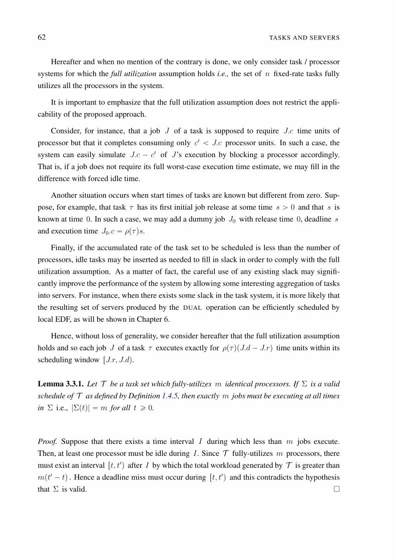
62 TASKS AND SERVERS
Hereafter and when no mention of the contrary is done, we only consider task / processor
systems for which the full utilization assumption holds i.e., the set of n fixed-rate tasks fully
utilizes all the processors in the system.
It is important to emphasize that the full utilization assumption does not restrict the appli-
cability of the proposed approach.
Consider, for instance, that a job J of a task is supposed to require J.c time units of
processor but that it completes consuming only c1 ă J.c processor units. In such a case, the
system can easily simulate J.c ´ c1 of J’s execution by blocking a processor accordingly.
That is, if a job does not require its full worst-case execution time estimate, we may fill in the
difference with forced idle time.
Another situation occurs when start times of tasks are known but different from zero. Sup-
pose, for example, that task τ has its first initial job release at some time s ą 0 and that s is
known at time 0. In such a case, we may add a dummy job J0 with release time 0, deadline s
and execution time J0.c “ ρpτqs.
Finally, if the accumulated rate of the task set to be scheduled is less than the number of
processors, idle tasks may be inserted as needed to fill in slack in order to comply with the full
utilization assumption. As a matter of fact, the careful use of any existing slack may signifi-
cantly improve the performance of the system by allowing some interesting aggregation of tasks
into servers. For instance, when there exists some slack in the task system, it is more likely that
the resulting set of servers produced by the DUAL operation can be efficiently scheduled by
local EDF, as will be shown in Chapter 6.
Hence, without loss of generality, we consider hereafter that the full utilization assumption
holds and so each job J of a task τ executes exactly for ρpτqpJ.d ´ J.rq time units within its
scheduling window rJ.r, J.dq.
Lemma 3.3.1. Let T be a task set which fully-utilizes m identical processors. If Σ is a valid
schedule of T as defined by Definition 1.4.5, then exactly m jobs must be executing at all times
in Σ i.e., |Σptq| “ m for all t ě 0.
Proof. Suppose that there exists a time interval I during which less than m jobs execute.
Then, at least one processor must be idle during I . Since T fully-utilizes m processors, there
must exist an interval rt, t1q after I by which the total workload generated by T is greater than
mpt1 ´ tq . Hence a deadline miss must occur during rt, t1q and this contradicts the hypothesis
that Σ is valid.
3.4 SERVERS 63
3.4 SERVERS
As mentioned in Section 1.7, the derivation of a schedule for a multiprocessor system will
be done by generating a schedule for a series of equivalent uniprocessor systems using the Dual
Scheduling Equivalence approach. But, prior to this, one may need to aggregate tasks into
servers via a PACK operation. However, since an aggregated task set must be feasible on a
single processor, we require that the rate of a server is not greater than one.
Hence, in this section we will not deal with the multiprocessor scheduling problem. The
focus here is on precisely defining the concept of server (Section 3.4.1) and showing that a
server correctly schedules the tasks associated to it (Section 3.4.2). In other words, one can
assume in this section that there is a single processor in the system. Later on we will show how
multiple servers are scheduled on a multiprocessor system by means of the Dual Scheduling
Equivalence approach.
3.4.1 Server model and notations
We treat servers as fixed-rate tasks with a sequence of jobs, but they are not actual tasks in
the system. In brief, each server can be seen as a proxy for a collection of client tasks that it
schedules according to an internal scheduling policy. Somehow abusively, we shall say that a
server is executing on a processor when the processor time is consumed by one of its clients.
We now give a precise definition of the server for a set of tasks.
Definition 3.4.1 (Server/Client). Let T be a set of fixed-rate tasks with total rate given by
ρpT q “ř
τPT ρpτq ď 1. A server S for T , denoted serpT q, is a virtual task with rate ρpT q,
release instant set RpSq “Ť
τPT Rpτq and equipped with a work-conserving scheduling policy
to schedule the tasks in T . A task in T is called an S’s client and T is the set of S’s clients,
also denoted clipSq.
We refer to a job of any client of S as a client job of S. If S is a server and Γ a set of
servers, then serpclipSqq “ S and clipserpΓqq “ Γ. Also, if S1 and S2 are two clients of the
same server S, then we say that S1 and S2 are siblings.
By Definition 3.4.1, the execution requirement of a server S in any interval rri, ri`1q equals
ρpSqpri`1´riq, where ri and ri`1 are consecutive release instants in RpSq. Then the workload
for job J of server S with J.r “ ri and J.d “ ri`1 equals J.c “ epJ, J.rq “ ρpSqpJ.d´J.rq,
just as with a “real” job.
However, just as a server S is a proxy for its clients, so too are the “jobs” of server S ,
which represent the budget allocated to S so that its clients’ jobs may execute. Hence, we
refer to a job JSi of server S as a budget job with the following interpretation. At each time
64 TASKS AND SERVERS
Γ p0.7q
Sp0.4q1
“ serptτ1uq
Sp0.3q2
“ serptτ2, τ3uq
Figure 3.2. A two-server set. The notation Xpρq means that ρpXq “ ρ.
ri in RpSq, server S replenishes its budget for the interval rri, ri`1q with ri`1 “ minttt P
RpSq, t ą riu by releasing a budget job JSi with JS
i .r “ ri and JSi .d “ ri`1. As a con-
sequence, at any given time t, the budget of S just equals epJSi , tq, where JS
i is the current
budget job of S at time t.
As will become clearer in Chapter 4, the PACK operation is an off-line procedure which
statically allocates tasks to servers. As a consequence, the client/server relationships are invari-
ant during an on-line schedule of the task system. This allows us to consistently define the rate
ρpSq of server S to be ρpclipSqq.
As an example, consider Figure 3.2, where Γ is a set comprised of the two servers S1 “
serptτ1uq and S2 “ serptτ2, τ3uq for the tasks τ1, and τ2 and τ3, respectively. If ρpτ1q “ 0.4,
ρpτ2q “ 0.2 and ρpτ3q “ 0.1, then ρpS1q “ 0.4 and ρpS2q “ 0.3. Also, if S “ serpΓq is the
server in charge of scheduling S1 and S2, then Γ “ clipSq “ tS1, S2u and ρpSq “ 0.7.
Note that since servers are themselves tasks, a set of servers of accumulated rate not greater
than one can be served by another “meta” server. Hence, we may speak of a server for a set of
servers. On the other hand, a server may have a single task as only client. In such a case, the
budget jobs of the server have the same deadlines and execution time as the “real” jobs of the
task. Since we assume that the scheduling policy of servers is work-conserving, there are no
difference between scheduling a single task τ or its dedicated server serptτuq. Hence, we see
that the concepts of fixed-rate task and server are largely interchangeable.
As task set with accumulated rate exactly equal to one will play a special role in this disser-
tation, we define a unit set and a unit server, both of which are feasible on a single processor.
Definition 3.4.2 (Unit Set/Unit Server). A set Γ of tasks/servers is a unit set if ρpΓq “ 1. The
server serpΓq for a unit set Γ is a unit server.
We say that a server meets its deadlines when all of its budget jobs meet theirs deadlines.
However, even if a server meets all its deadlines, it must use an appropriate scheduling policy
to ensure that its clients meet theirs.
For example, consider two periodic tasks τ1 :r12, 2Ns and τ2 :r13, 3Ns , with periods
equal to 2 and 3 and rates ρpτ1q “ 12 and ρpτ2q “ 13, respectively. Assume a synchronous
task system, i.e., start times equal to zero. Consider a server S scheduling these two tasks on
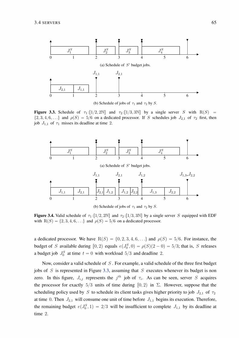
3.4 SERVERS 65
0 1 2 3 4 5 6
JS1
JS2
JS3
JS4
(a) Schedule of S’ budget jobs.
0 1 2 3 4 5 6
J2,1 J1,1
J1,1 J2,1
(b) Schedule of jobs of τ1 and τ2 by S.
Figure 3.3. Schedule of τ1 :r12, 2Ns and τ2 :r13, 3Ns by a single server S with RpSq “t2, 3, 4, 6, . . .u and ρpSq “ 56 on a dedicated processor. If S schedules job J2,1 of τ2 first, thenjob J1,1 of τ1 misses its deadline at time 2.
0 1 2 3 4 5 6
JS1
JS2
JS3
JS4
(a) Schedule of S’ budget jobs.
0 1 2 3 4 5 6
J1,1 J2,1 J2,1 J1,2 J1,2 J2,2 J1,3 J2,2
J1,1 J2,1 J1,2 J1,3,J2,2
(b) Schedule of jobs of τ1 and τ2 by S.
Figure 3.4. Valid schedule of τ1 :r12, 2Ns and τ2 :r13, 3Ns by a single server S equipped with EDFwith RpSq “ t2, 3, 4, 6, . . .u and ρpSq “ 56 on a dedicated processor.
a dedicated processor. We have RpSq “ t0, 2, 3, 4, 6, . . .u and ρpSq “ 56. For instance, the
budget of S available during r0, 2q equals epJS0, 0q “ ρpSqp2 ´ 0q “ 53; that is, S releases
a budget job JS0
at time t “ 0 with workload 53 and deadline 2.
Now, consider a valid schedule of S . For example, a valid schedule of the three first budget
jobs of S is represented in Figure 3.3, assuming that S executes whenever its budget is non
zero. In this figure, Ji,j represents the jth job of τi. As can be seen, server S acquires
the processor for exactly 53 units of time during r0, 2q in Σ. However, suppose that the
scheduling policy used by S to schedule its client tasks gives higher priority to job J2,1 of τ2at time 0. Then J2,1 will consume one unit of time before J1,1 begins its execution. Therefore,
the remaining budget epJS0, 1q “ 23 will be insufficient to complete J1,1 by its deadline at
time 2.
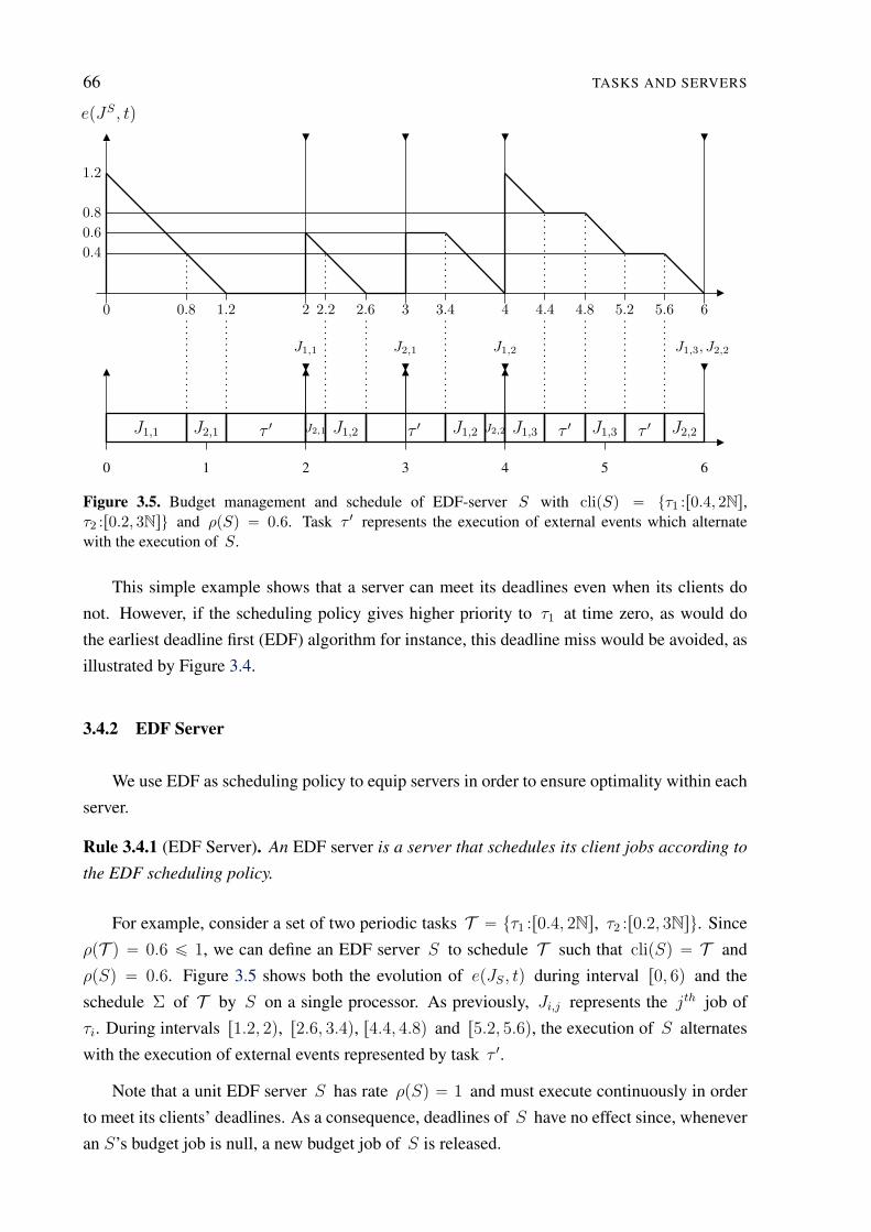
66 TASKS AND SERVERS
epJS, tq
0 0.8 1.2 2 2.2 2.6 3 3.4 4 4.4 4.8 5.2 5.6 6
1.2
0.6
0.8
0.4
0 1 2 3 4 5 6
J1,1 J2,1 τ 1 J2,1 J1,2 τ 1 J1,2 J2,2 J1,3 τ 1 J1,3 τ 1 J2,2
J1,1 J1,2J2,1 J1,3, J2,2
Figure 3.5. Budget management and schedule of EDF-server S with clipSq “ tτ1 :r0.4, 2Ns,τ2 :r0.2, 3Nsu and ρpSq “ 0.6. Task τ 1 represents the execution of external events which alternatewith the execution of S.
This simple example shows that a server can meet its deadlines even when its clients do
not. However, if the scheduling policy gives higher priority to τ1 at time zero, as would do
the earliest deadline first (EDF) algorithm for instance, this deadline miss would be avoided, as
illustrated by Figure 3.4.
3.4.2 EDF Server
We use EDF as scheduling policy to equip servers in order to ensure optimality within each
server.
Rule 3.4.1 (EDF Server). An EDF server is a server that schedules its client jobs according to
the EDF scheduling policy.
For example, consider a set of two periodic tasks T “ tτ1 :r0.4, 2Ns, τ2 :r0.2, 3Nsu. Since
ρpT q “ 0.6 ď 1, we can define an EDF server S to schedule T such that clipSq “ T and
ρpSq “ 0.6. Figure 3.5 shows both the evolution of epJS, tq during interval r0, 6q and the
schedule Σ of T by S on a single processor. As previously, Ji,j represents the jth job of
τi. During intervals r1.2, 2q, r2.6, 3.4q, r4.4, 4.8q and r5.2, 5.6q, the execution of S alternates
with the execution of external events represented by task τ 1.
Note that a unit EDF server S has rate ρpSq “ 1 and must execute continuously in order
to meet its clients’ deadlines. As a consequence, deadlines of S have no effect since, whenever
an S’s budget job is null, a new budget job of S is released.
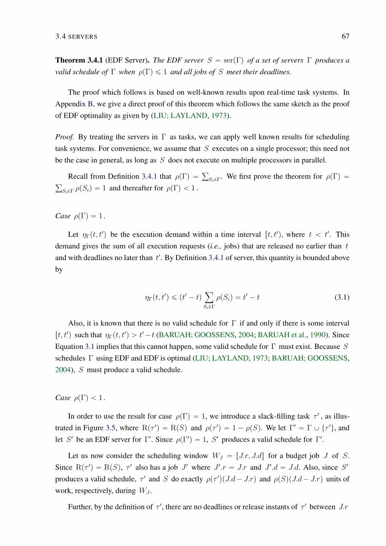
3.4 SERVERS 67
Theorem 3.4.1 (EDF Server). The EDF server S “ serpΓq of a set of servers Γ produces a
valid schedule of Γ when ρpΓq ď 1 and all jobs of S meet their deadlines.
The proof which follows is based on well-known results upon real-time task systems. In
Appendix B, we give a direct proof of this theorem which follows the same sketch as the proof
of EDF optimality as given by (LIU; LAYLAND, 1973).
Proof. By treating the servers in Γ as tasks, we can apply well known results for scheduling
task systems. For convenience, we assume that S executes on a single processor; this need not
be the case in general, as long as S does not execute on multiple processors in parallel.
Recall from Definition 3.4.1 that ρpΓq “ř
SiPΓ. We first prove the theorem for ρpΓq “
ř
SiPΓρpSiq “ 1 and thereafter for ρpΓq ă 1 .
Case ρpΓq “ 1 .
Let ηΓpt, t1q be the execution demand within a time interval rt, t1q, where t ă t1. This
demand gives the sum of all execution requests (i.e., jobs) that are released no earlier than t
and with deadlines no later than t1. By Definition 3.4.1 of server, this quantity is bounded above
by
ηΓpt, t1q ď pt1 ´ tqÿ
SiPΓ
ρpSiq “ t1 ´ t (3.1)
Also, it is known that there is no valid schedule for Γ if and only if there is some interval
rt, t1q such that ηΓpt, t1q ą t1 ´ t (BARUAH; GOOSSENS, 2004; BARUAH et al., 1990). Since
Equation 3.1 implies that this cannot happen, some valid schedule for Γ must exist. Because S
schedules Γ using EDF and EDF is optimal (LIU; LAYLAND, 1973; BARUAH; GOOSSENS,
2004), S must produce a valid schedule.
Case ρpΓq ă 1 .
In order to use the result for case ρpΓq “ 1, we introduce a slack-filling task τ 1 , as illus-
trated in Figure 3.5, where Rpτ 1q “ RpSq and ρpτ 1q “ 1 ´ ρpSq. We let Γ1 “ Γ Y tτ 1u, and
let S 1 be an EDF server for Γ1. Since ρpΓ1q “ 1, S 1 produces a valid schedule for Γ1.
Let us now consider the scheduling window WJ “ rJ.r, J.ds for a budget job J of S.
Since Rpτ 1q “ RpSq, τ 1 also has a job J 1 where J 1.r “ J.r and J 1.d “ J.d. Also, since S 1
produces a valid schedule, τ 1 and S do exactly ρpτ 1qpJ.d´ J.rq and ρpSqpJ.d´ J.rq units of
work, respectively, during WJ .
Further, by the definition of τ 1, there are no deadlines or release instants of τ 1 between J.r
68 TASKS AND SERVERS
and J.d. Consequently, the workload of τ 1 may be arbitrarily rearranged or subdivided within
the interval WJ without compromising the correctness of the schedule. Also, we may do this
for all budget jobs of S so as to reproduce any schedule of S where it meets its deadlines.
Finally, since S and S 1 both schedule tasks in Γ with EDF, S will produce the same valid
schedule for Γ as S 1, giving our desired result.
3.5 PARTIAL KNOWLEDGE
As first pointed by Greg Levin in (REGNIER et al., 2011), a server can correctly schedule
its clients without the need to “know” all arrival times of its clients’ jobs at the outset. Indeed,
the assumed system model only requires that there are no gaps or overlaps between jobs of task
or server. In other words, the deadline of a job of a task or server is the release instant of the
next job of the same task or server. As a consequence, at any time, the knowledge of the earliest
deadline of an EDF server S’s clients is the minimum and sufficient information that S needs
to take scheduling decision for its clients.
In practice, this knowledge is sufficient in order for a server to estimate its budget job for
its next scheduling window. In other words, the required and sufficient knowledge horizon of a
server is its next deadline. This is an important distinction with the PPID task model. Indeed,
unlike periodic tasks where all deadlines are known at the outset, the fixed-rate task model
allows for jobs whose complete set of deadlines is not known a priori.
However, the rates and first release instants of tasks and servers are parameters which must
be known prior the execution of the system.
3.6 PARTITIONED PROPORTIONATE FAIRNESS
Unlike previous Proportionate Fairness (Pfair) based approaches, client tasks scheduled by
servers do not receive their proportional shares between each system deadline nor between each
server deadline. Instead, each aggregating server responsible for scheduling a group of servers,
is guaranteed a constant processor bandwidth. Hence, according to the Partitioned Proportion-
ate Fairness approach (PP-Fair), the total bandwidth available in the system is “fairly” shared
between all aggregating servers, each of which is
i) guaranteed a budget proportional to the sum of its clients’ rates between any two consec-
utive deadlines of its clients;
ii) responsible for scheduling its clients in some correct fashion (e.g., EDF) between such
deadlines.
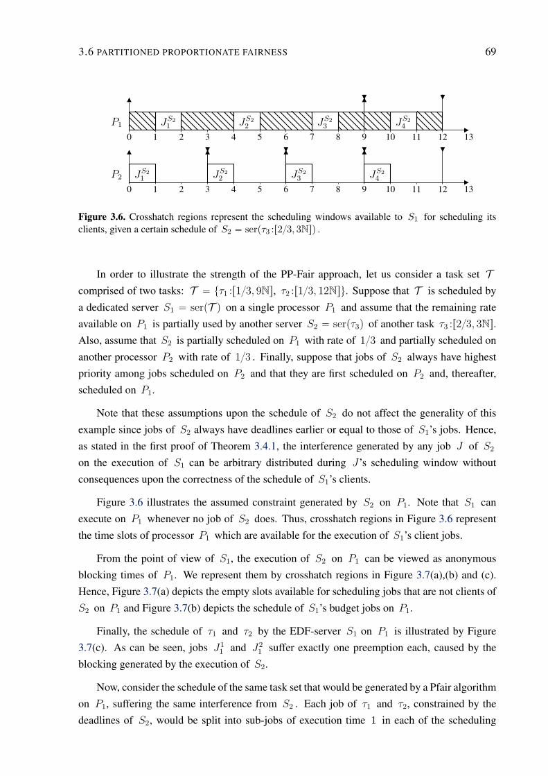
3.6 PARTITIONED PROPORTIONATE FAIRNESS 69
0 1 2 3 4 5 6 7 8 9 10 11 12 13
P1 JS2
1JS2
2JS2
3JS2
4
0 1 2 3 4 5 6 7 8 9 10 11 12 13
P2 JS2
1JS2
2JS2
3JS2
4
Figure 3.6. Crosshatch regions represent the scheduling windows available to S1 for scheduling itsclients, given a certain schedule of S2 “ serpτ3 :r23, 3Nsq .
In order to illustrate the strength of the PP-Fair approach, let us consider a task set T
comprised of two tasks: T “ tτ1 :r13, 9Ns, τ2 :r13, 12Nsu. Suppose that T is scheduled by
a dedicated server S1 “ serpT q on a single processor P1 and assume that the remaining rate
available on P1 is partially used by another server S2 “ serpτ3q of another task τ3 :r23, 3Ns.
Also, assume that S2 is partially scheduled on P1 with rate of 13 and partially scheduled on
another processor P2 with rate of 13 . Finally, suppose that jobs of S2 always have highest
priority among jobs scheduled on P2 and that they are first scheduled on P2 and, thereafter,
scheduled on P1.
Note that these assumptions upon the schedule of S2 do not affect the generality of this
example since jobs of S2 always have deadlines earlier or equal to those of S1’s jobs. Hence,
as stated in the first proof of Theorem 3.4.1, the interference generated by any job J of S2
on the execution of S1 can be arbitrary distributed during J’s scheduling window without
consequences upon the correctness of the schedule of S1’s clients.
Figure 3.6 illustrates the assumed constraint generated by S2 on P1. Note that S1 can
execute on P1 whenever no job of S2 does. Thus, crosshatch regions in Figure 3.6 represent
the time slots of processor P1 which are available for the execution of S1’s client jobs.
From the point of view of S1, the execution of S2 on P1 can be viewed as anonymous
blocking times of P1. We represent them by crosshatch regions in Figure 3.7(a),(b) and (c).
Hence, Figure 3.7(a) depicts the empty slots available for scheduling jobs that are not clients of
S2 on P1 and Figure 3.7(b) depicts the schedule of S1’s budget jobs on P1.
Finally, the schedule of τ1 and τ2 by the EDF-server S1 on P1 is illustrated by Figure
3.7(c). As can be seen, jobs J1
1and J2
1suffer exactly one preemption each, caused by the
blocking generated by the execution of S2.
Now, consider the schedule of the same task set that would be generated by a Pfair algorithm
on P1, suffering the same interference from S2 . Each job of τ1 and τ2, constrained by the
deadlines of S2, would be split into sub-jobs of execution time 1 in each of the scheduling
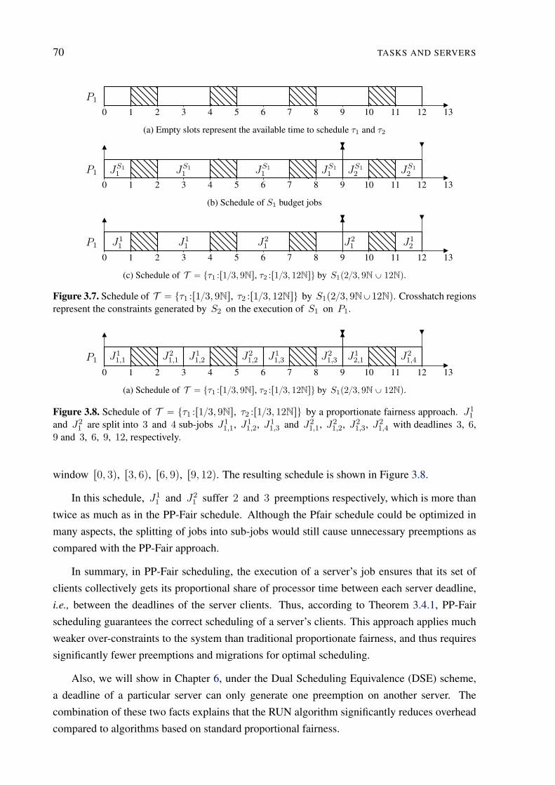
70 TASKS AND SERVERS
0 1 2 3 4 5 6 7 8 9 10 11 12 13
P1
(a) Empty slots represent the available time to schedule τ1 and τ2
0 1 2 3 4 5 6 7 8 9 10 11 12 13
P1 JS1
1JS1
1JS1
1JS1
1JS1
2JS1
2
(b) Schedule of S1 budget jobs
0 1 2 3 4 5 6 7 8 9 10 11 12 13
P1 J1
1J1
1J2
1J2
1J1
2
(c) Schedule of T “ tτ1 :r13, 9Ns, τ2 :r13, 12Nsu by S1p23, 9N Y 12Nq.
Figure 3.7. Schedule of T “ tτ1 :r13, 9Ns, τ2 :r13, 12Nsu by S1p23, 9NY12Nq. Crosshatch regionsrepresent the constraints generated by S2 on the execution of S1 on P1.
0 1 2 3 4 5 6 7 8 9 10 11 12 13
P1J1
1,1 J2
1,1 J1
1,2 J2
1,2 J1
1,3 J2
1,3 J1
2,1 J2
1,4
(a) Schedule of T “ tτ1 :r13, 9Ns, τ2 :r13, 12Nsu by S1p23, 9N Y 12Nq.
Figure 3.8. Schedule of T “ tτ1 :r13, 9Ns, τ2 :r13, 12Nsu by a proportionate fairness approach. J11
and J21
are split into 3 and 4 sub-jobs J11,1, J1
1,2, J11,3 and J2
1,1, J21,2, J2
1,3, J21,4 with deadlines 3, 6,
9 and 3, 6, 9, 12, respectively.
window r0, 3q, r3, 6q, r6, 9q, r9, 12q. The resulting schedule is shown in Figure 3.8.
In this schedule, J1
1and J2
1suffer 2 and 3 preemptions respectively, which is more than
twice as much as in the PP-Fair schedule. Although the Pfair schedule could be optimized in
many aspects, the splitting of jobs into sub-jobs would still cause unnecessary preemptions as
compared with the PP-Fair approach.
In summary, in PP-Fair scheduling, the execution of a server’s job ensures that its set of
clients collectively gets its proportional share of processor time between each server deadline,
i.e., between the deadlines of the server clients. Thus, according to Theorem 3.4.1, PP-Fair
scheduling guarantees the correct scheduling of a server’s clients. This approach applies much
weaker over-constraints to the system than traditional proportionate fairness, and thus requires
significantly fewer preemptions and migrations for optimal scheduling.
Also, we will show in Chapter 6, under the Dual Scheduling Equivalence (DSE) scheme,
a deadline of a particular server can only generate one preemption on another server. The
combination of these two facts explains that the RUN algorithm significantly reduces overhead
compared to algorithms based on standard proportional fairness.
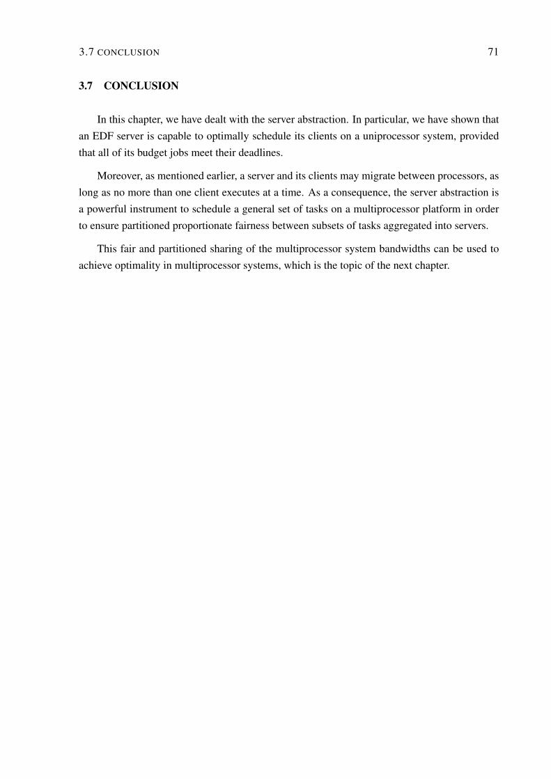
3.7 CONCLUSION 71
3.7 CONCLUSION
In this chapter, we have dealt with the server abstraction. In particular, we have shown that
an EDF server is capable to optimally schedule its clients on a uniprocessor system, provided
that all of its budget jobs meet their deadlines.
Moreover, as mentioned earlier, a server and its clients may migrate between processors, as
long as no more than one client executes at a time. As a consequence, the server abstraction is
a powerful instrument to schedule a general set of tasks on a multiprocessor platform in order
to ensure partitioned proportionate fairness between subsets of tasks aggregated into servers.
This fair and partitioned sharing of the multiprocessor system bandwidths can be used to
achieve optimality in multiprocessor systems, which is the topic of the next chapter.

72 TASKS AND SERVERS
Chapter
4Virtual Scheduling by reduction to uniprocessor ensures partitioned proportionate fairness (PP-Fair), which im-
poses a less restrictive set of constraints than those imposed by proportionate fairness (Pfair) for scheduling peri-
odic real-time tasks in multiprocessors. PP-Fairness can be achieved by the composition of duality and packing.
Moreover, this efficient combination allows for reducing a general task system with integer utilization greater than
or equal to two to a system of unit servers which can be efficiently scheduled on uniprocessor systems.
VIRTUAL SCHEDULING
In this chapter, we describe three operations, DUAL, PACK and REDUCE, which iteratively re-
duce the number of processors in a multiprocessor fixed-rate task or server system until a set of
uniprocessor server systems is obtained.
At execution time, the schedules for these unit servers are generated by the EDF scheduling
policy. Then, from these uniprocessor schedules, the corresponding schedule for the original
multiprocessor fixed-rate task system is deduced straightforwardly by following simple rules.
4.1 INTRODUCTION
As introduced in Section 1.7, the DUAL operation transforms a server S into the dual server
S˚, whose execution time represents the idle time of S. Since ρpS˚q “ 1 ´ ρpSq, the DUAL
operation reduces the total rate and the number of required processors in systems where most
tasks have high rates, i.e., rates close or equal to one. Also, we will see in Section 4.2 that the
Dual Scheduling Equivalence (DSE) can be efficiently used to deduce a valid schedule for those
particular sets of high-rate servers from the schedule of the set of their dual servers.
Next, we will show in Section 4.3 that such high-rate servers can always be generated via a
PACK operation. Indeed, sets of tasks whose rates sum to no more than one can be packed into
servers, reducing the number of tasks and producing the high-rate servers needed by the DSE
rule.
73
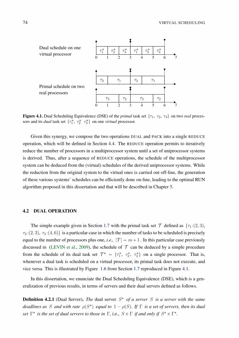
74 VIRTUAL SCHEDULING
0 1 2 3 4 5 6 7
Dual schedule on onevirtual processor
τ˚1
τ˚2
τ˚3
τ˚1
τ˚2
τ˚3
Primal schedule on tworeal processors
0 1 2 3 4 5 6 7
τ3
τ2
τ2
τ1
τ3
τ2
τ2
τ1
Figure 4.1. Dual Scheduling Equivalence (DSE) of the primal task set tτ1, τ2, τ3u on two real proces-sors and its dual task set tτ˚
1, τ˚
2τ˚3
u on one virtual processor.
Given this synergy, we compose the two operations DUAL and PACK into a single REDUCE
operation, which will be defined in Section 4.4. The REDUCE operation permits to iteratively
reduce the number of processors in a multiprocessor system until a set of uniprocessor systems
is derived. Thus, after a sequence of REDUCE operations, the schedule of the multiprocessor
system can be deduced from the (virtual) schedules of the derived uniprocessor systems. While
the reduction from the original system to the virtual ones is carried out off-line, the generation
of these various systems’ schedules can be efficiently done on-line, leading to the optimal RUN
algorithm proposed in this dissertation and that will be described in Chapter 5.
4.2 DUAL OPERATION
The simple example given in Section 1.7 with the primal task set T defined as tτ1 :p2, 3q,
τ2 :p2, 3q, τ3 :p4, 6qu is a particular case in which the number of tasks to be scheduled is precisely
equal to the number of processors plus one, i.e., |T | “ m`1 . In this particular case previously
discussed in (LEVIN et al., 2009), the schedule of T can be deduced by a simple procedure
from the schedule of its dual task set T ˚ “ tτ˚1
, τ˚2
, τ˚3
u on a single processor. That is,
whenever a dual task is scheduled on a virtual processor, its primal task does not execute, and
vice versa. This is illustrated by Figure 1.6 from Section 1.7 reproduced in Figure 4.1.
In this dissertation, we enunciate the Dual Scheduling Equivalence (DSE), which is a gen-
eralization of previous results, in terms of servers and their dual servers defined as follows.
Definition 4.2.1 (Dual Server). The dual server S˚ of a server S is a server with the same
deadlines as S and with rate ρpS˚q equal to 1 ´ ρpSq. If Γ is a set of servers, then its dual
set Γ˚ is the set of dual servers to those in Γ, i.e., S P Γ if and only if S˚ P Γ˚.
4.2 DUAL OPERATION 75
Note that the dual server of a primal unit server S, which has rate ρpSq “ 1 and must
execute continuously in order to meet its clients’ deadlines, is a null server, which has rate
ρpSq “ 0 and never executes.
As usual with duality, the relation pS˚q˚ “ S holds. Hereafter, S is referred to as the
primal server of its dual server S˚. We now enunciate the definition of the dual schedule of a
schedule of primal servers.
Definition 4.2.2 (Dual Schedule). Let Γ be a set of primal servers and Γ˚ be its dual set. Two
schedules Σ of Γ and Σ˚ of Γ˚ are duals if, for all times t and all S P Γ, S P Σptq if and
only if S˚ R Σ˚ptq; that is, S executes exactly when S˚ is idle, and vice versa.
Like for servers, Γ, and Σ are referred to as primal relative to their duals Γ˚, and Σ˚.
Here again, pΓ˚q˚ “ Γ and pΣ˚q˚ “ Σ. As a matter of fact, this latter identity is our main
motivation for adopting the unusual definition of schedule as given in Section 1.4.1. Indeed,
recall that according to Definition 1.4.1, a schedule does not specify on which processor each
server executes at any time as usual in real-time literature. Instead, a schedule of a set of servers
Γ just specifies which subset of servers in Γ execute at any time. Then, the assignment of
the subset of server jobs’ chosen to execute on the processors is done by the job-to-processor
assignment step as previously described in Section 1.4.3.
This disjunction between the scheduling step and the job-to-processor assignment step is
which allows for the identity pΣ˚q˚ “ Σ to be true, as expected for any “good” notion of
duality.
We now establish the Dual Scheduling Equivalence (DSE) which states that the schedule
of a primal set of servers is valid precisely when its dual schedule is valid. This equivalence
is enunciated for server set with integer rate. However, this assumption does not imply any
loss of generality. Indeed, consider a set of servers Γ with non-integer accumulated rate ρpΓq.
The minimal integer m of processors needed to feasibly schedule Γ equals tρpΓqu ` 1. As
previously explained in Section 3.3, we can complete Γ to obtain an integer accumulated rate
task system, by adding a slack-filling server of rate m ´ ρpΓq. Thus, the result presented here
can be applied to any server system with non-integer rate by filling it to achieve an integer rate.
Theorem 4.2.1 (Dual Scheduling Equivalence). Let Γ be a set of n “ m ` k servers with
k ě 1 and such that the accumulated rate ρpΓq of Γ equals m, an integer. Consider a
schedule Σ of Γ on m processors and let Σ˚ and Γ˚ be the duals of Σ and Γ, respectively.
Then ρpΓ˚q “ k, and so Γ˚ is feasible on k processors. Further, Σ is valid if and only if Σ˚
is valid.
76 VIRTUAL SCHEDULING
Proof. First,
ρpΓ˚q “ÿ
S˚PΓ˚
ρpS˚q
“ÿ
SPΓ
p1 ´ ρpSqq
“ n ´ ρpΓq
“ k
so k processors are sufficient to feasibly schedule Γ˚. Next, we prove that if Σ is valid for Γ
then Definitions 1.4.1 and 1.4.5 implies that Σ˚ is valid for Γ˚ .
Because Σ is a valid schedule on m processors and we assume full utilization, Σ always
executes m distinct tasks as shown by Lemma 3.3.1. The remaining k “ n ´ m tasks are
idle in Σ, and so are exactly the tasks executing in Σ˚. Hence Σ˚ is always executing exactly
k distinct tasks on its k (virtual) processors. Also, since Σ is valid, any job J of server
S P Γ does exactly J.c “ ρpSqpJ.d ´ J.rq units of work between its release instant J.r
and its deadline J.d. During this same time, S˚ has a matching job J˚ where J˚.r “ J.r,
J˚.d “ J.d, and
J˚.c “ ρpS˚qpJ˚.d ´ J˚.rq
“ p1 ´ ρpSqqpJ.d ´ J.rq
“ pJ.d ´ J.rq ´ J.c
That is, J˚’s execution time during the interval rJ.d, J.rq is exactly the length of time that J
must be idle. Thus, as J executes for J.c during this interval in Σ, J˚ executes for J˚.c in
Σ˚. Consequently, J˚ satisfies condition (ii) of Definition 1.4.1 and also meets its deadline.
Since this holds for all jobs of all dual servers, Σ˚ is a valid schedule for Γ˚.
The converse also follows from the above argument, since pΣ˚q˚ “ Σ.
Once again, see Figure 4.1 for a simple illustration. We now summarize this dual scheduling
rule for future reference.
Rule 4.2.1 (Dual Scheduling Equivalence). At any time, execute in Σ the servers of Γ whose
dual servers are not executing in Σ˚, and vice versa.
Finally, we define the DUAL operation ϕ as follows.
Definition 4.2.3 (DUAL Operation). The DUAL operation ϕ from a set of servers Γ to its dual
set Γ˚ is the bijection which associates a server S with its dual server S˚, i.e., ϕpSq “ S˚.
4.3 PACK OPERATION 77
In this dissertation, we adopt the usual definition for the image of a subset. That is, if
f : E Ñ F is a mapping from E to F and G Ď E is a subset of E, then the image fpGq of
G by f is defined as
fpGq “ tfpxq, x P Gu
For example, if Γ is a set of server, then the dual set of Γ is ϕpΓq “ tS˚, S P Γu “ Γ˚.
It is important to emphasize that Theorem 4.2.1 does not establish any scheduling rule to
generate feasible schedules. It only states that determining a valid schedule for a given server
set on m processors is equivalent to finding a valid schedule for the transformed set on n´m
virtual processors. Nonetheless, this theorem raises an interesting issue. Indeed, dealing with
n´m virtual processors instead of m can be advantageous if n´m ă m. In order to illustrate
this observation, consider our example set of three servers with utilization equal to 23. Instead
of searching for a valid schedule on two processors, one can focus on the schedule of the dual
servers on just one virtual processor, a problem whose solution is well known.
In order to guarantee that dealing with dual servers is indeed advantageous, the PACK oper-
ation plays a central role.
4.3 PACK OPERATION
As seen in the previous section, the DUAL operation is a powerful mechanism to reduce the
number of processors but it only works properly if n´m ă m where n and m are the number
of tasks and processors respectively. However, this is not the case for general task sets.
Consider for instance a simple set T of 5 tasks, all with rate 25 . Here, n “ 5 , m “
ρpT q “ 2 and n ´ m “ 3 ą 2. In such a case, directly applying duality does not simplify the
scheduling problem. Indeed, the dual T ˚ of T is comprised of 5 task all of which with rate
1 ´ 25 “ 35. Hence, the accumulated rate of T ˚ equals 3, which is greater than the initial
number of processors needed to schedule T . Hence, the DUAL operation directly applied to T
leads to a more complex problem than the primal one.
As can be deduced from this simple example, whenever n ´ m ě m, one needs to reduce
the number of tasks/servers to be scheduled, aggregating them into servers. This is achieved by
the PACK operation that we properly define in this section.
Definition 4.3.1 (Packing). Let Γ be a set of servers. A partition tΓ1, Γ2, . . ., Γku of Γ is a
packing of Γ if ρpΓiq ď 1 for all i and ρpΓiq ` ρpΓjq ą 1 for all i ‰ j. An algorithm A is
a packing algorithm if it partitions any set of servers into a packing. In such a case, we denote
the packing of Γ produced by A as πArΓs.
An illustrative example is given by Figure 4.2, where the three sets Γ1, Γ2 and Γ3 show a
packing of the set Γ of 7 servers.
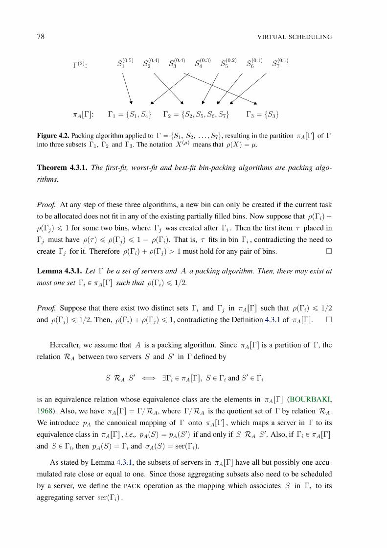
78 VIRTUAL SCHEDULING
Γp2q: Sp0.5q1
Sp0.4q2
Sp0.4q3
Sp0.3q4
Sp0.2q5
Sp0.1q6
Sp0.1q7
πArΓs: Γ1 “ tS1, S4u Γ2 “ tS2, S5, S6, S7u Γ3 “ tS3u
Figure 4.2. Packing algorithm applied to Γ “ tS1, S2, . . . , S7u, resulting in the partition πArΓs of Γ
into three subsets Γ1, Γ2 and Γ3. The notation Xpµq means that ρpXq “ µ.
Theorem 4.3.1. The first-fit, worst-fit and best-fit bin-packing algorithms are packing algo-
rithms.
Proof. At any step of these three algorithms, a new bin can only be created if the current task
to be allocated does not fit in any of the existing partially filled bins. Now suppose that ρpΓiq `
ρpΓjq ď 1 for some two bins, where Γj was created after Γi . Then the first item τ placed in
Γj must have ρpτq ď ρpΓjq ď 1 ´ ρpΓiq. That is, τ fits in bin Γi , contradicting the need to
create Γj for it. Therefore ρpΓiq ` ρpΓjq ą 1 must hold for any pair of bins.
Lemma 4.3.1. Let Γ be a set of servers and A a packing algorithm. Then, there may exist at
most one set Γi P πArΓs such that ρpΓiq ď 12.
Proof. Suppose that there exist two distinct sets Γi and Γj in πArΓs such that ρpΓiq ď 12
and ρpΓjq ď 12. Then, ρpΓiq ` ρpΓjq ď 1, contradicting the Definition 4.3.1 of πArΓs.
Hereafter, we assume that A is a packing algorithm. Since πArΓs is a partition of Γ, the
relation RA between two servers S and S 1 in Γ defined by
S RA S 1 ðñ DΓi P πArΓs, S P Γi and S 1 P Γi
is an equivalence relation whose equivalence class are the elements in πArΓs (BOURBAKI,
1968). Also, we have πArΓs “ ΓRA, where ΓRA is the quotient set of Γ by relation RA.
We introduce pA the canonical mapping of Γ onto πArΓs , which maps a server in Γ to its
equivalence class in πArΓs , i.e., pApSq “ pApS 1q if and only if S RA S 1. Also, if Γi P πArΓs
and S P Γi, then pApSq “ Γi and σApSq “ serpΓiq.
As stated by Lemma 4.3.1, the subsets of servers in πArΓs have all but possibly one accu-
mulated rate close or equal to one. Since those aggregating subsets also need to be scheduled
by a server, we define the PACK operation as the mapping which associates S in Γi to its
aggregating server serpΓiq .
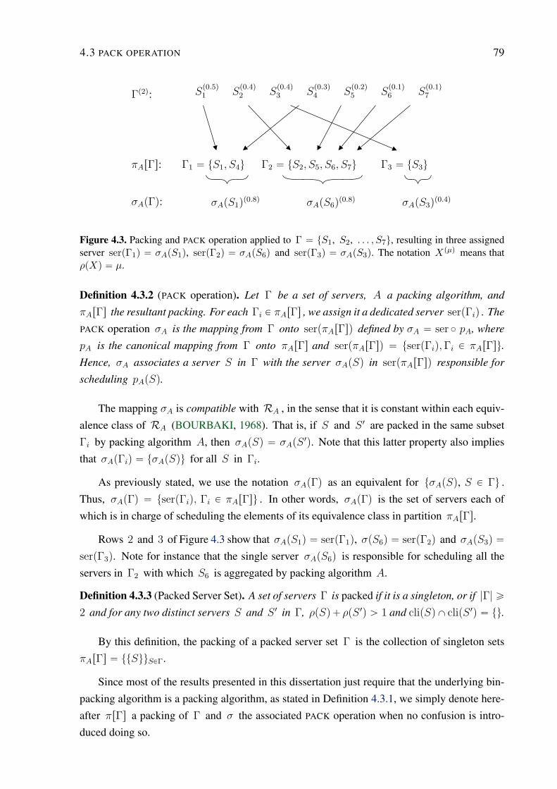
4.3 PACK OPERATION 79
Γp2q: Sp0.5q1
Sp0.4q2
Sp0.4q3
Sp0.3q4
Sp0.2q5
Sp0.1q6
Sp0.1q7
πArΓs:
σApΓq:
Γ1 “ tS1, S4u
σApS1qp0.8q
Γ2 “ tS2, S5, S6, S7u
σApS6qp0.8q
Γ3 “ tS3u
σApS3qp0.4q
Figure 4.3. Packing and PACK operation applied to Γ “ tS1, S2, . . . , S7u, resulting in three assignedserver serpΓ1q “ σApS1q, serpΓ2q “ σApS6q and serpΓ3q “ σApS3q. The notation Xpµq means thatρpXq “ µ.
Definition 4.3.2 (PACK operation). Let Γ be a set of servers, A a packing algorithm, and
πArΓs the resultant packing. For each Γi P πArΓs , we assign it a dedicated server serpΓiq . The
PACK operation σA is the mapping from Γ onto serpπArΓsq defined by σA “ ser ˝ pA, where
pA is the canonical mapping from Γ onto πArΓs and serpπArΓsq “ tserpΓiq,Γi P πArΓsu.
Hence, σA associates a server S in Γ with the server σApSq in serpπArΓsq responsible for
scheduling pApSq.
The mapping σA is compatible with RA , in the sense that it is constant within each equiv-
alence class of RA (BOURBAKI, 1968). That is, if S and S 1 are packed in the same subset
Γi by packing algorithm A, then σApSq “ σApS 1q. Note that this latter property also implies
that σApΓiq “ tσApSqu for all S in Γi.
As previously stated, we use the notation σApΓq as an equivalent for tσApSq, S P Γu .
Thus, σApΓq “ tserpΓiq, Γi P πArΓsu . In other words, σApΓq is the set of servers each of
which is in charge of scheduling the elements of its equivalence class in partition πArΓs.
Rows 2 and 3 of Figure 4.3 show that σApS1q “ serpΓ1q, σpS6q “ serpΓ2q and σApS3q “
serpΓ3q. Note for instance that the single server σApS6q is responsible for scheduling all the
servers in Γ2 with which S6 is aggregated by packing algorithm A.
Definition 4.3.3 (Packed Server Set). A set of servers Γ is packed if it is a singleton, or if |Γ| ě
2 and for any two distinct servers S and S 1 in Γ, ρpSq `ρpS 1q ą 1 and clipSq X clipS 1q “ tu.
By this definition, the packing of a packed server set Γ is the collection of singleton sets
πArΓs “ ttSuuSPΓ.
Since most of the results presented in this dissertation just require that the underlying bin-
packing algorithm is a packing algorithm, as stated in Definition 4.3.1, we simply denote here-
after πrΓs a packing of Γ and σ the associated PACK operation when no confusion is intro-
duced doing so.
80 VIRTUAL SCHEDULING
4.4 REDUCE OPERATION
We now compose the DUAL and PACK operations, as defined in 4.2.3 and 4.3.2 respectively,
into the REDUCE operation. As will be shown, a sequence of reductions transforms a multipro-
cessor scheduling problem to a collection of uniprocessor scheduling problems. Hence, the
REDUCE operation can be viewed as a cornerstone of the RUN algorithm presented in this dis-
sertation.
In order to see the effectiveness of the composition of the PACK and DUAL operations, we
first establish a lemma which characterizes the convergence of this composition in terms of
server set cardinality.
Lemma 4.4.1. Let Γ be a packed set of servers, and let ϕpΓq be the dual set of Γ . Suppose
we apply a PACK operation σ to ϕpΓq. Then
|σ ˝ϕpΓq | ď
R
|Γ| ` 1
2
V
.
Proof. Let n “ |Γ|. Since Γ is packed, there is at most one server S in Γ such that ρpSq ď
12 (by Lemma 4.3.1). This implies that at least n ´ 1 servers in ϕpΓq have rates less than
12. When these n ´ 1 dual servers are packed, they will be, at a minimum, paired off. Thus,
π will pack ϕpΓq into at most rpn ´ 1q2s ` 1 subsets. Hence,
|σ ˝ϕpΓq| ď
R
n ` 1
2
V
.
Thus, packing the dual of a packed set reduces the number of servers by about half. Since
we will use this pair of operations repeatedly, we define a REDUCE operation to be their com-
position.
Definition 4.4.1 (REDUCE Operation). Given a set of servers Γ and a packing algorithm A, a
REDUCE operation on a server S in Γ, denoted ψpSq, is the composition of the DUAL operation
ϕ with the PACK operation σ associated with A, i.e., ψ “ ϕ˝σ.
Figure 4.4 illustrates the steps of the REDUCE operation ψ. As we intend to apply REDUCE
repeatedly until we are left with only one or more unit servers, we now define a reduction
sequence.
Definition 4.4.2 (Reduction Level/Sequence). Let i ě 1 be an integer, Γ a set of servers,
and S a server in Γ. The operator ψi is recursively defined by ψ0pSq “ S and ψipSq “
ψ ˝ψi´1pSq. tψiui is a reduction sequence, and the server system ψipΓq is said to be at
reduction level i.
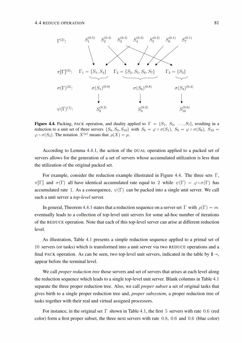
4.4 REDUCE OPERATION 81
Γp2q: Sp0.5q1
Sp0.4q2
Sp0.4q3
Sp0.3q4
Sp0.2q5
Sp0.1q6
Sp0.1q7
πrΓsp2q:
σpΓqp2q:
Γ1 “ tS1, S4u
σpS1qp0.8q
Γ2 “ tS2, S5, S6, S7u
σpS6qp0.8q
Γ3 “ tS3u
σpS3qp0.4q
ψpΓqp1q: Sp0.2q8
Sp0.2q9
Sp0.6q10
Figure 4.4. Packing, PACK operation, and duality applied to Γ “ tS1, S2, . . . , S7u, resulting in areduction to a unit set of three servers tS8, S9, S10u with S8 “ ϕ ˝ σpS1q, S9 “ ϕ ˝ σpS6q, S10 “ϕ ˝ σpS3q. The notation Xpµq means that ρpXq “ µ.
According to Lemma 4.4.1, the action of the DUAL operation applied to a packed set of
servers allows for the generation of a set of servers whose accumulated utilization is less than
the utilization of the original packed set.
For example, consider the reduction example illustrated in Figure 4.4. The three sets Γ,
πrΓs and σpΓq all have identical accumulated rate equal to 2 while ψpΓq “ ϕ˝σpΓq has
accumulated rate 1. As a consequence, ψpΓq can be packed into a single unit server. We call
such a unit server a top-level server.
In general, Theorem 4.4.1 states that a reduction sequence on a server set Γ with ρpΓq “ m
eventually leads to a collection of top-level unit servers for some ad-hoc number of iterations
of the REDUCE operation. Note that each of this top-level server can arise at different reduction
level.
As illustration, Table 4.1 presents a simple reduction sequence applied to a primal set of
10 servers (or tasks) which is transformed into a unit server via two REDUCE operations and a
final PACK operation. As can be seen, two top-level unit servers, indicated in the table by 1Ñ,
appear before the terminal level.
We call proper reduction tree those servers and set of servers that arises at each level along
the reduction sequence which leads to a single top-level unit server. Blank columns in Table 4.1
separate the three proper reduction tree. Also, we call proper subset a set of original tasks that
gives birth to a single proper reduction tree and, proper subsystem, a proper reduction tree of
tasks together with their real and virtual assigned processors.
For instance, in the original set Γ shown in Table 4.1, the first 5 servers with rate 0.6 (red
color) form a first proper subset, the three next servers with rate 0.8, 0.6 and 0.6 (blue color)
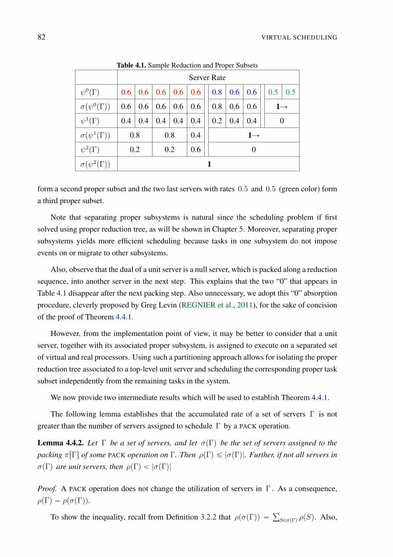
82 VIRTUAL SCHEDULING
Table 4.1. Sample Reduction and Proper Subsets
Server Rate
ψ0pΓq 0.6 0.6 0.6 0.6 0.6 0.8 0.6 0.6 0.5 0.5
σpψ0pΓqq 0.6 0.6 0.6 0.6 0.6 0.8 0.6 0.6 1Ñ
ψ1pΓq 0.4 0.4 0.4 0.4 0.4 0.2 0.4 0.4 0
σpψ1pΓqq 0.8 0.8 0.4 1Ñ
ψ2pΓq 0.2 0.2 0.6 0
σpψ2pΓqq 1
form a second proper subset and the two last servers with rates 0.5 and 0.5 (green color) form
a third proper subset.
Note that separating proper subsystems is natural since the scheduling problem if first
solved using proper reduction tree, as will be shown in Chapter 5. Moreover, separating proper
subsystems yields more efficient scheduling because tasks in one subsystem do not impose
events on or migrate to other subsystems.
Also, observe that the dual of a unit server is a null server, which is packed along a reduction
sequence, into another server in the next step. This explains that the two “0” that appears in
Table 4.1 disappear after the next packing step. Also unnecessary, we adopt this “0” absorption
procedure, cleverly proposed by Greg Levin (REGNIER et al., 2011), for the sake of concision
of the proof of Theorem 4.4.1.
However, from the implementation point of view, it may be better to consider that a unit
server, together with its associated proper subsystem, is assigned to execute on a separated set
of virtual and real processors. Using such a partitioning approach allows for isolating the proper
reduction tree associated to a top-level unit server and scheduling the corresponding proper task
subset independently from the remaining tasks in the system.
We now provide two intermediate results which will be used to establish Theorem 4.4.1.
The following lemma establishes that the accumulated rate of a set of servers Γ is not
greater than the number of servers assigned to schedule Γ by a PACK operation.
Lemma 4.4.2. Let Γ be a set of servers, and let σpΓq be the set of servers assigned to the
packing πrΓs of some PACK operation on Γ. Then ρpΓq ď |σpΓq|. Further, if not all servers in
σpΓq are unit servers, then ρpΓq ă |σpΓq|
Proof. A PACK operation does not change the utilization of servers in Γ . As a consequence,
ρpΓq “ ρpσpΓqq.
To show the inequality, recall from Definition 3.2.2 that ρpσpΓqq “ř
SPσpΓq ρpSq. Also,
4.4 REDUCE OPERATION 83
since ρpSq ď 1 for all servers S in σpΓq and
ÿ
SPσpΓq
1 “ |σpΓq|,
it follows that ρpσpΓqq ď |σpΓq|. Moreover, if not all servers in σpΓq are unit server, then there
exists at least one server S in σpΓq such that ρpSq ă 1 and the inequality is strict.
Lemma 4.4.3. Let Γ be a packed set of servers, not all of which are unit servers. If ρpΓq is a
positive integer, then |Γ| ě 3.
Proof. If Γ “ tS1u and S1 is not a unit server, then ρpΓq ă 1, not a positive integer. If
Γ “ tS1, S2u is a packed set, then ρpΓq “ ρpS1q ` ρpS2q ą 1; but ρpΓq is not 2 unless S1
and S2 are both unit servers. Thus |Γ| is not 1 or 2.
Theorem 4.4.1 (Reduction Convergence). Let Γ be a set of servers where ρpΓq is a positive
integer. Then for some p ě 0, σpψppΓqq is a set of unit servers.
Proof. We prove the theorem by finite induction on the number k of reduction level.
Let Γpkq “ ψkpΓq and suppose that ρpΓkq is a positive integer. If σpΓkq is a set of unit
servers, then p “ k and the induction is finished.
Otherwise, according to Lemma 4.4.3, |σpΓkq| ě 3. Next, consider Γk`1 “ ψk`1pΓq and
observe that
σpΓk`1q “ σ ˝ψk`1pΓq
“ σ ˝ψ ˝ψkpΓq
“ σ ˝ϕ˝σpΓpkqq
“ pσ ˝ϕqpσpΓpkqqq
Since σpΓkq is a packed set of servers, Lemma 4.4.1 tells us that
σpΓk`1q ď
R
|σpΓkq| ` 1
2
V
.
Since |σpΓkq| ě 3 and rpx ` 1q2s ă x for x ě 3, we deduce that
|σpΓk`1q| ă |σpΓkq|
Now, recall we assume that ρpσpΓkqq is a positive integer. Moreover, since σpΓkq are not all
unit servers, it follows from Lemma 4.4.2 that ρpσpΓkqq ă |σpΓkq| .
Further, Theorem 4.2.1 implies that ρpϕpσpΓkqqq is also a positive integer; as is
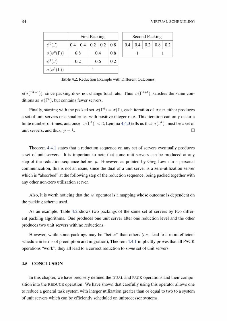
84 VIRTUAL SCHEDULING
First Packing Second Packing
ψ0pΓq 0.4 0.4 0.2 0.2 0.8 0.4 0.4 0.2 0.8 0.2
σpψ0pΓqq 0.8 0.4 0.8 1 1
ψ1pΓq 0.2 0.6 0.2
σpψ1pΓqq 1
Table 4.2. Reduction Example with Different Outcomes.
ρpσpΓk`1qq, since packing does not change total rate. Thus σpΓk`1q satisfies the same con-
ditions as σpΓkq, but contains fewer servers.
Finally, starting with the packed set σpΓ0q “ σpΓq, each iteration of σ ˝ϕ either produces
a set of unit servers or a smaller set with positive integer rate. This iteration can only occur a
finite number of times, and once |σpΓkq| ă 3, Lemma 4.4.3 tells us that σpΓkq must be a set of
unit servers, and thus, p “ k.
Theorem 4.4.1 states that a reduction sequence on any set of servers eventually produces
a set of unit servers. It is important to note that some unit servers can be produced at any
step of the reduction sequence before p. However, as pointed by Greg Levin in a personal
communication, this is not an issue, since the dual of a unit server is a zero-utilization server
which is “absorbed” at the following step of the reduction sequence, being packed together with
any other non-zero utilization server.
Also, it is worth noticing that the ψ operator is a mapping whose outcome is dependent on
the packing scheme used.
As an example, Table 4.2 shows two packings of the same set of servers by two differ-
ent packing algorithms. One produces one unit server after one reduction level and the other
produces two unit servers with no reductions.
However, while some packings may be “better” than others (i.e., lead to a more efficient
schedule in terms of preemption and migration), Theorem 4.4.1 implicitly proves that all PACK
operations “work”; they all lead to a correct reduction to some set of unit servers.
4.5 CONCLUSION
In this chapter, we have precisely defined the DUAL and PACK operations and their compo-
sition into the REDUCE operation. We have shown that carefully using this operator allows one
to reduce a general task system with integer utilization greater than or equal to two to a system
of unit servers which can be efficiently scheduled on uniprocessor systems.
4.5 CONCLUSION 85
However, one must observe that the REDUCE operation applied to a set of task does not
tell us anything about the on-line scheduling of that tasks. As a matter of fact, the reduction
sequence associated to a given packing can be determined off-line.
Thereafter, one must combine the Dual Scheduling Equivalence and the server schedul-
ing policy, assumed to be EDF in this dissertation, in order to deduce from the uniprocessor
schedules of the reduced server system an on-line schedule of the primal set of tasks.
In the next chapter, we focus on proper set of tasks for which a reduction sequence produces
a single unit server. For such sets, we show how one can use the associated proper reduction
tree to generate an on-line schedule of the primal tasks.
In general, the RUN scheduling algorithm can be used to schedule many proper subsystems,
since each of these subsystems are independent and can be scheduled in an isolated manner.

86 VIRTUAL SCHEDULING
Chapter
5An adequate sequence of REDUCE operations transforms a general multiprocessor primal task system into a set
of one or more unit servers which can be schedule on virtual uniprocessor systems. Then, the on-line schedule
of the primal multiprocessor task system can be deduced from the (virtual) schedules of the derived uniprocessor
systems. This is performed by combining the Dual Scheduling Equivalence and the EDF server scheduling policy.
REDUCTION TO UNIPROCESSOR (RUN)
5.1 INTRODUCTION
In Chapters 1, 3 and 4, we have described our real-time system model, namely the fixed-rate
task model as defined in Definition 3.2.1 for identical processors. We also have introduced new
abstractions, namely the EDF server abstraction as defined in Definition 3.4.1 and the operations
DUAL, PACK and REDUCE as defined in Definitions 4.2.3, 4.3.2 and 4.4.1, respectively. Hence,
we can now describe the reduction to uniprocessor (RUN) scheduling algorithm which is the
main contribution of this dissertation.
RUN is based on the original notion of partitioned proportionate fairness (PP-Fair), as
introduced in Section 1.7. PP-Fairness imposes a less restrictive set of constraints when com-
pared to those present in the notion of proportionate fairness (Pfair) from (BARUAH et al.,
1993), which has been used in previous optimal solutions for the problem of scheduling peri-
odic real-time tasks on multiprocessors up to now. Indeed, to the best of our knowledge, RUN
is the first optimal multiprocessor scheduling algorithm for periodic real-time task systems not
based on proportionate fairness.
Recall from Chapter 4 that the REDUCE operation is the composition of the DUAL and
PACK operations. First, the PACK operation, precisely defined in Section 4.3 of Chapter 4,
transforms a set of low-rate tasks compared to one into a set of high-rate servers compared to
one. Indeed, those sets of tasks whose rates sum up to no more than one are packed into servers,
reducing the number of tasks and producing a packed set of high-rate servers needed to apply
the Dual Scheduling Equivalence (DSE) rule. Second, the DUAL operation, precisely defined in
87
88 REDUCTION TO UNIPROCESSOR (RUN)
Section 4.2 of Chapter 4, transforms a server S into its dual server S˚, whose execution time
represents the idle time of S i.e., ρpS˚q “ 1´ρpSq. Then, given a schedule of the dual system
of a primal system of high-rate servers, the DSE rule allows for deducing a valid schedule for
the primal set of servers.
For some particular task system, this sequence of operations may need to be iterated, as first
pointed out by Ernesto Massa in (REGNIER et al., 2011), in order to obtain a set of unit servers,
each of which is feasible on a uniprocessor system. Hence, carefully composing the DUAL
and PACK operators into the REDUCE operator allows one to achieve partitioned proportional
fairness by reduction of any general periodic task system with integer accumulated rate greater
than or equal to two to a system of unit servers.
However, one must observe that the REDUCE operation applied to a primal set of tasks
does not tell us anything about the on-line scheduling of those tasks. As a matter of fact, the
reduction sequence associated to a given packing can be carried out off-line. As an interest-
ing consequence, given some particular goal, one can look for a packing with nice properties
according to this specific goal in off-line/during design time.
In this chapter, we show how the on-line schedule of the multiprocessor system can be
deduced from the (virtual) schedules of the derived uniprocessor systems. This is performed
by combining the Dual Scheduling Equivalence and the EDF server scheduling policy in order
to deduce from the uniprocessor schedules of the reduced server system an on-line schedule
of the primal set of tasks. This procedure leads us to the detailed presentation of RUN, the
multiprocessor on-line and optimal scheduling algorithm for periodic task systems proposed in
this dissertation.
For the sake of simplicity of this chapter, we focus on proper set of tasks for which a
reduction sequence produces a single unit server. For such sets, we show how one can use
the associated proper reduction tree to generate an on-line schedule of the primal tasks. This
simplification does not cause any loss of generality since, if more than one proper subsystem
are needed for the reduction of a general primal task system into proper subsystems, then each
of these proper subsystems can be scheduled in an isolated and independent way by the RUN
scheduling algorithm.
Structure of the chapter
Section 5.2 describes the RUN scheduling procedure and the associated on-line scheduling
rules while Section 5.3 depicts an alternative interpretation of the RUN tree, which may be
helpful for future works, as for example, a RUN based solution for the sporadic task model.
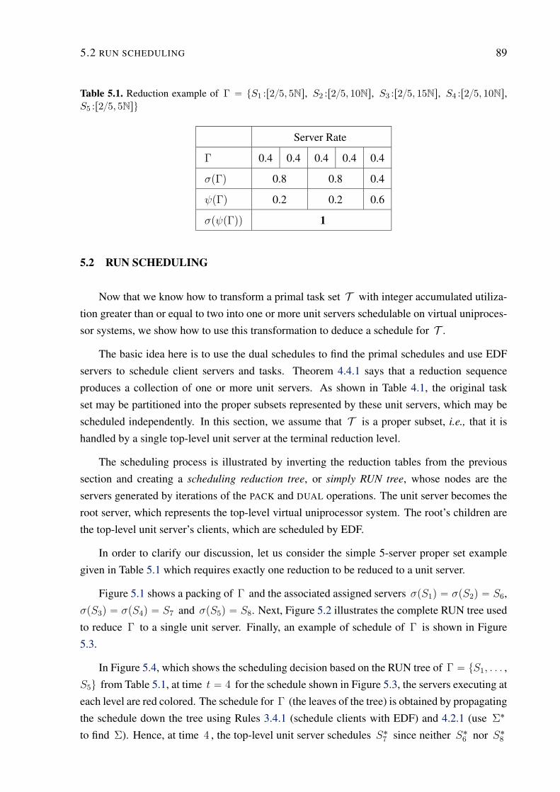
5.2 RUN SCHEDULING 89
Table 5.1. Reduction example of Γ “ tS1 :r25, 5Ns, S2 :r25, 10Ns, S3 :r25, 15Ns, S4 :r25, 10Ns,S5 :r25, 5Nsu
Server Rate
Γ 0.4 0.4 0.4 0.4 0.4
σpΓq 0.8 0.8 0.4
ψpΓq 0.2 0.2 0.6
σpψpΓqq 1
5.2 RUN SCHEDULING
Now that we know how to transform a primal task set T with integer accumulated utiliza-
tion greater than or equal to two into one or more unit servers schedulable on virtual uniproces-
sor systems, we show how to use this transformation to deduce a schedule for T .
The basic idea here is to use the dual schedules to find the primal schedules and use EDF
servers to schedule client servers and tasks. Theorem 4.4.1 says that a reduction sequence
produces a collection of one or more unit servers. As shown in Table 4.1, the original task
set may be partitioned into the proper subsets represented by these unit servers, which may be
scheduled independently. In this section, we assume that T is a proper subset, i.e., that it is
handled by a single top-level unit server at the terminal reduction level.
The scheduling process is illustrated by inverting the reduction tables from the previous
section and creating a scheduling reduction tree, or simply RUN tree, whose nodes are the
servers generated by iterations of the PACK and DUAL operations. The unit server becomes the
root server, which represents the top-level virtual uniprocessor system. The root’s children are
the top-level unit server’s clients, which are scheduled by EDF.
In order to clarify our discussion, let us consider the simple 5-server proper set example
given in Table 5.1 which requires exactly one reduction to be reduced to a unit server.
Figure 5.1 shows a packing of Γ and the associated assigned servers σpS1q “ σpS2q “ S6,
σpS3q “ σpS4q “ S7 and σpS5q “ S8. Next, Figure 5.2 illustrates the complete RUN tree used
to reduce Γ to a single unit server. Finally, an example of schedule of Γ is shown in Figure
5.3.
In Figure 5.4, which shows the scheduling decision based on the RUN tree of Γ “ tS1, . . . ,
S5u from Table 5.1, at time t “ 4 for the schedule shown in Figure 5.3, the servers executing at
each level are red colored. The schedule for Γ (the leaves of the tree) is obtained by propagating
the schedule down the tree using Rules 3.4.1 (schedule clients with EDF) and 4.2.1 (use Σ˚
to find Σ). Hence, at time 4 , the top-level unit server schedules S˚7
since neither S˚6
nor S˚8
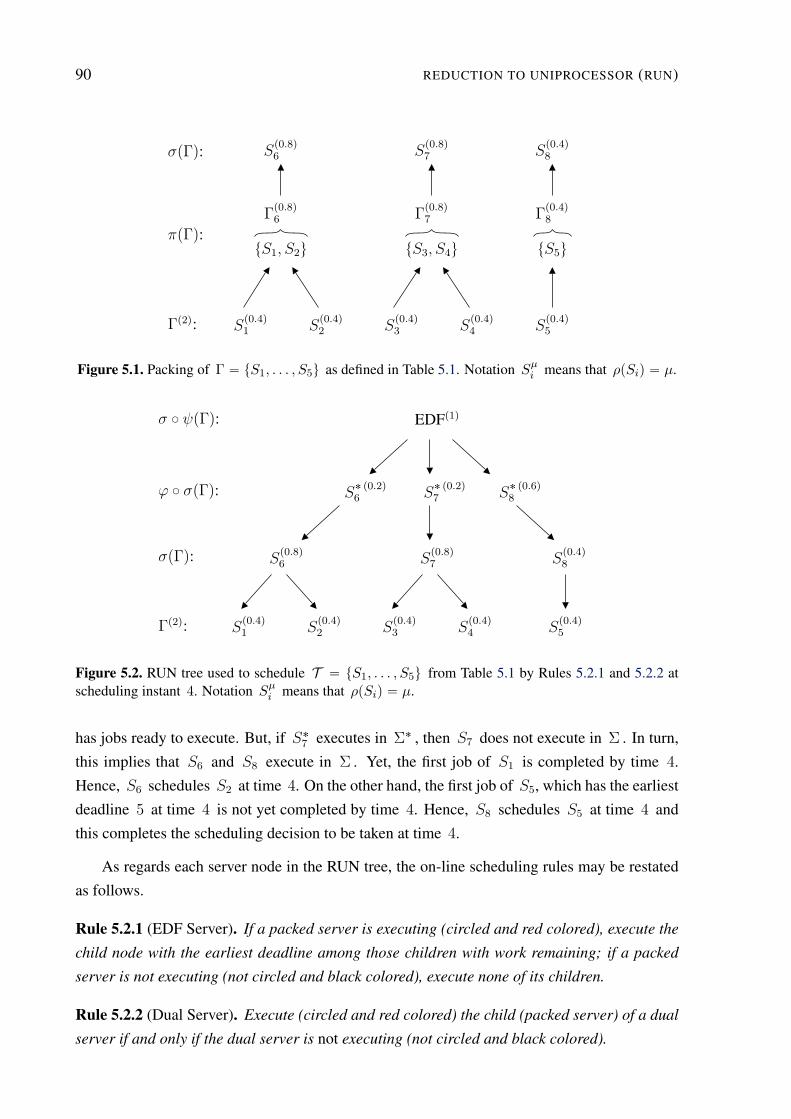
90 REDUCTION TO UNIPROCESSOR (RUN)
σpΓq:
πpΓq:
Sp0.8q6
Γp0.8q6
tS1, S2u
Sp0.8q7
Γp0.8q7
tS3, S4u
Sp0.4q8
Γp0.4q8
tS5u
Γp2q: Sp0.4q1
Sp0.4q2
Sp0.4q3
Sp0.4q4
Sp0.4q5
Figure 5.1. Packing of Γ “ tS1, . . . , S5u as defined in Table 5.1. Notation Sµi means that ρpSiq “ µ.
σ ˝ ψpΓq: EDFp1q
ϕ ˝ σpΓq: S˚ p0.2q6
S˚ p0.2q7
S˚ p0.6q8
σpΓq: Sp0.8q6
Sp0.8q7
Sp0.4q8
Γp2q: Sp0.4q1
Sp0.4q2
Sp0.4q3
Sp0.4q4
Sp0.4q5
Figure 5.2. RUN tree used to schedule T “ tS1, . . . , S5u from Table 5.1 by Rules 5.2.1 and 5.2.2 atscheduling instant 4. Notation S
µi means that ρpSiq “ µ.
has jobs ready to execute. But, if S˚7
executes in Σ˚ , then S7 does not execute in Σ . In turn,
this implies that S6 and S8 execute in Σ . Yet, the first job of S1 is completed by time 4.
Hence, S6 schedules S2 at time 4. On the other hand, the first job of S5, which has the earliest
deadline 5 at time 4 is not yet completed by time 4. Hence, S8 schedules S5 at time 4 and
this completes the scheduling decision to be taken at time 4.
As regards each server node in the RUN tree, the on-line scheduling rules may be restated
as follows.
Rule 5.2.1 (EDF Server). If a packed server is executing (circled and red colored), execute the
child node with the earliest deadline among those children with work remaining; if a packed
server is not executing (not circled and black colored), execute none of its children.
Rule 5.2.2 (Dual Server). Execute (circled and red colored) the child (packed server) of a dual
server if and only if the dual server is not executing (not circled and black colored).
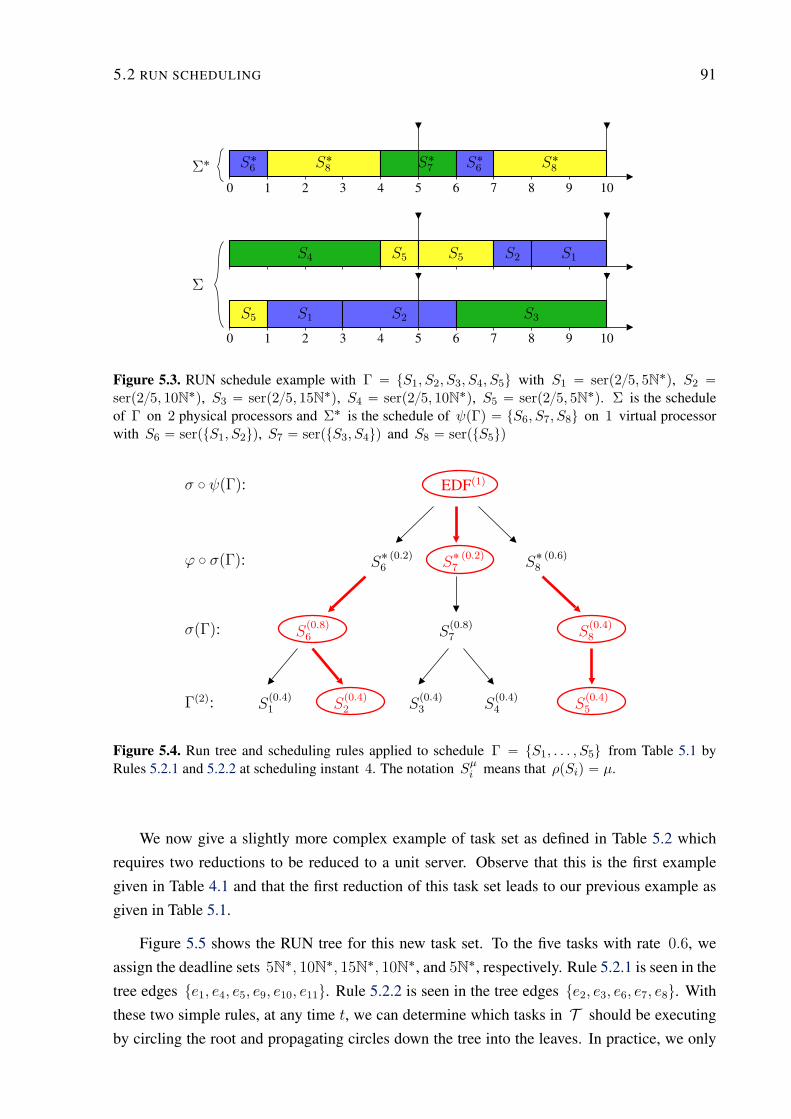
5.2 RUN SCHEDULING 91
Σ˚
0 1 2 3 4 5 6 7 8 9 10
S˚6
S˚8
S˚7
S˚6
S˚8
Σ
0 1 2 3 4 5 6 7 8 9 10
S4 S5 S5 S2 S1
S5 S1 S2 S3
Figure 5.3. RUN schedule example with Γ “ tS1, S2, S3, S4, S5u with S1 “ serp25, 5N˚q, S2 “serp25, 10N˚q, S3 “ serp25, 15N˚q, S4 “ serp25, 10N˚q, S5 “ serp25, 5N˚q. Σ is the scheduleof Γ on 2 physical processors and Σ˚ is the schedule of ψpΓq “ tS6, S7, S8u on 1 virtual processorwith S6 “ serptS1, S2uq, S7 “ serptS3, S4uq and S8 “ serptS5uq
σ ˝ ψpΓq: EDFp1q
ϕ ˝ σpΓq: S˚ p0.2q6
S˚ p0.2q7
S˚ p0.6q8
σpΓq: Sp0.8q6
Sp0.8q7
Sp0.4q8
Γp2q: Sp0.4q1
Sp0.4q2
Sp0.4q3
Sp0.4q4
Sp0.4q5
Figure 5.4. Run tree and scheduling rules applied to schedule Γ “ tS1, . . . , S5u from Table 5.1 byRules 5.2.1 and 5.2.2 at scheduling instant 4. The notation S
µi means that ρpSiq “ µ.
We now give a slightly more complex example of task set as defined in Table 5.2 which
requires two reductions to be reduced to a unit server. Observe that this is the first example
given in Table 4.1 and that the first reduction of this task set leads to our previous example as
given in Table 5.1.
Figure 5.5 shows the RUN tree for this new task set. To the five tasks with rate 0.6, we
assign the deadline sets 5N˚, 10N˚, 15N˚, 10N˚, and 5N˚, respectively. Rule 5.2.1 is seen in the
tree edges te1, e4, e5, e9, e10, e11u. Rule 5.2.2 is seen in the tree edges te2, e3, e6, e7, e8u. With
these two simple rules, at any time t, we can determine which tasks in T should be executing
by circling the root and propagating circles down the tree into the leaves. In practice, we only
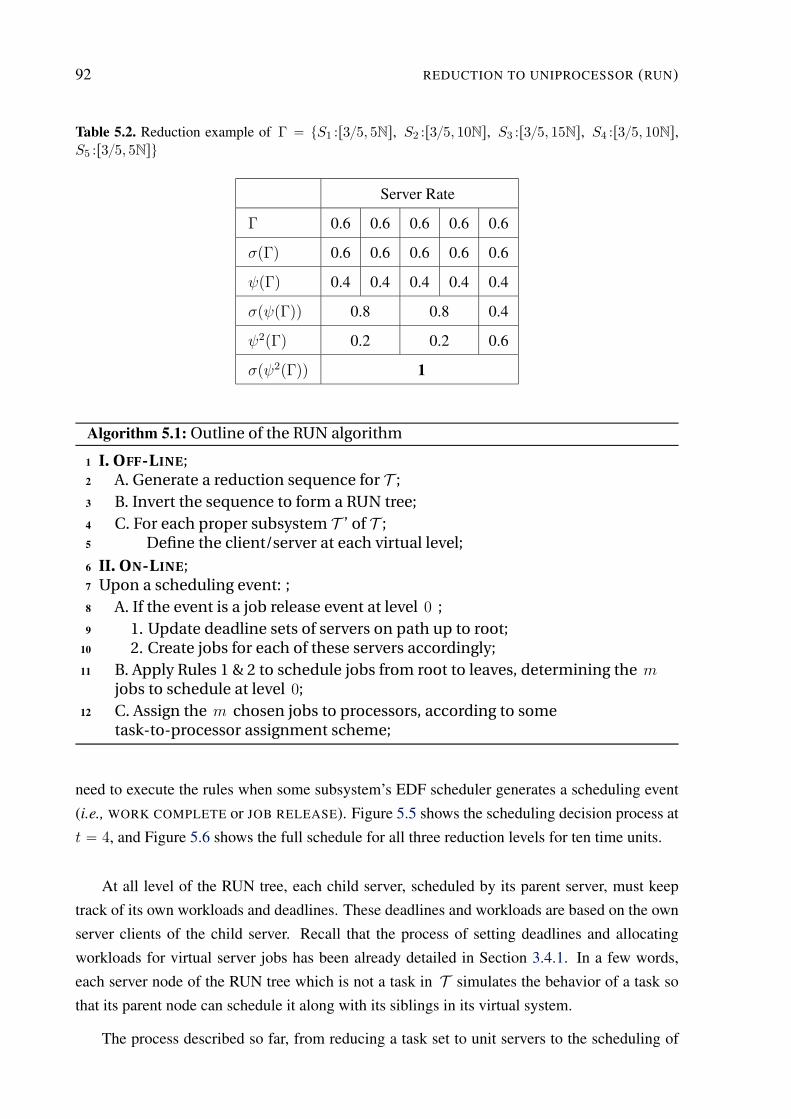
92 REDUCTION TO UNIPROCESSOR (RUN)
Table 5.2. Reduction example of Γ “ tS1 :r35, 5Ns, S2 :r35, 10Ns, S3 :r35, 15Ns, S4 :r35, 10Ns,S5 :r35, 5Nsu
Server Rate
Γ 0.6 0.6 0.6 0.6 0.6
σpΓq 0.6 0.6 0.6 0.6 0.6
ψpΓq 0.4 0.4 0.4 0.4 0.4
σpψpΓqq 0.8 0.8 0.4
ψ2pΓq 0.2 0.2 0.6
σpψ2pΓqq 1
Algorithm 5.1: Outline of the RUN algorithm
1 I. OFF-LINE;2 A. Generate a reduction sequence for T ;
3 B. Invert the sequence to form a RUN tree;
4 C. For each proper subsystem T ’ of T ;5 Define the client/server at each virtual level;
6 II. ON-LINE;7 Upon a scheduling event: ;
8 A. If the event is a job release event at level 0 ;
9 1. Update deadline sets of servers on path up to root;10 2. Create jobs for each of these servers accordingly;
11 B. Apply Rules 1 & 2 to schedule jobs from root to leaves, determining the m
jobs to schedule at level 0;
12 C. Assign the m chosen jobs to processors, according to sometask-to-processor assignment scheme;
need to execute the rules when some subsystem’s EDF scheduler generates a scheduling event
(i.e., WORK COMPLETE or JOB RELEASE). Figure 5.5 shows the scheduling decision process at
t “ 4, and Figure 5.6 shows the full schedule for all three reduction levels for ten time units.
At all level of the RUN tree, each child server, scheduled by its parent server, must keep
track of its own workloads and deadlines. These deadlines and workloads are based on the own
server clients of the child server. Recall that the process of setting deadlines and allocating
workloads for virtual server jobs has been already detailed in Section 3.4.1. In a few words,
each server node of the RUN tree which is not a task in T simulates the behavior of a task so
that its parent node can schedule it along with its siblings in its virtual system.
The process described so far, from reducing a task set to unit servers to the scheduling of
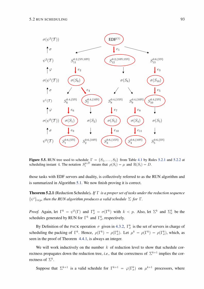
5.2 RUN SCHEDULING 93
σpψ2pT qq EDFp1q
σ e1
ψ2pT q S0.2,t5N,10Nu11
S0.2,t10N,15Nu12
S0.6,t5Nu13
ϕ e2 e3
σpψ1pT qq σpS6q σpS8q σpS10q
σ e4 e5
ψ1pT q S0.4,t5Nu6
S0.4,t10Nu7
S0.4,t15Nu8
S0.4,t10Nu9
S0.4,t5Nu10
ϕ e6 e7 e8
σpψ0pT qq σpS1q σpS2q σpS3q σpS4q σpS5q
σ e9 e10 e11
ψ0pT q S0.6,t5Nu1
S0.6,t10Nu2
S0.6,t15Nu3
S0.6,t10Nu4
S0.6,t5Nu5
Figure 5.5. RUN tree used to schedule Γ “ tS1, . . . , S5u from Table 4.1 by Rules 5.2.1 and 5.2.2 atscheduling instant 4. The notation S
µ,Di means that ρpSiq “ µ and RpSiq “ D.
those tasks with EDF servers and duality, is collectively referred to as the RUN algorithm and
is summarized in Algorithm 5.1. We now finish proving it is correct.
Theorem 5.2.1 (Reduction Schedule). If Γ is a proper set of tasks under the reduction sequence
tψiuiďp, then the RUN algorithm produces a valid schedule Σ for Γ.
Proof. Again, let Γk “ ψkpΓq and Γkσ “ σpΓkq with k ă p. Also, let Σk and Σk
σ be the
schedules generated by RUN for Γk and Γkσ, respectively.
By Definition of the PACK operation σ given in 4.3.2, Γkσ is the set of servers in charge of
scheduling the packing of Γk. Hence, ρpΓkq “ ρpΓkσq. Let µk “ ρpΓkq “ ρpΓk
σq, which, as
seen in the proof of Theorem 4.4.1, is always an integer.
We will work inductively on the number k of reduction level to show that schedule cor-
rectness propagates down the reduction tree, i.e., that the correctness of Σk`1 implies the cor-
rectness of Σk.
Suppose that Σk`1 is a valid schedule for Γk`1 “ ϕpΓkσq on µk`1 processors, where
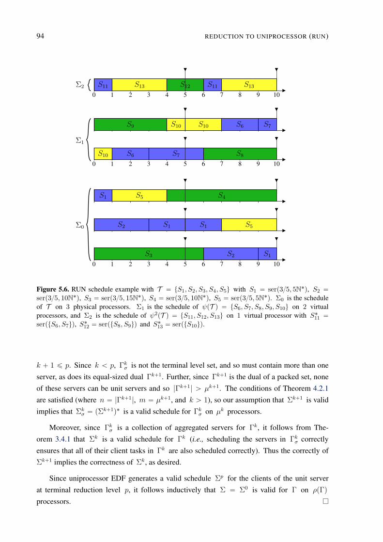
94 REDUCTION TO UNIPROCESSOR (RUN)
Σ2
0 1 2 3 4 5 6 7 8 9 10
S11 S13 S12 S11 S13
Σ1
0 1 2 3 4 5 6 7 8 9 10
S9 S10 S10 S6 S7
S10 S6 S7 S8
Σ0
0 1 2 3 4 5 6 7 8 9 10
S1 S5 S4
S2 S1 S1 S5
S3 S2 S1
Figure 5.6. RUN schedule example with T “ tS1, S2, S3, S4, S5u with S1 “ serp35, 5N˚q, S2 “serp35, 10N˚q, S3 “ serp35, 15N˚q, S4 “ serp35, 10N˚q, S5 “ serp35, 5N˚q. Σ0 is the scheduleof T on 3 physical processors. Σ1 is the schedule of ψpT q “ tS6, S7, S8, S9, S10u on 2 virtualprocessors, and Σ2 is the schedule of ψ2pT q “ tS11, S12, S13u on 1 virtual processor with S˚
11“
serptS6, S7uq, S˚12
“ serptS8, S9uq and S˚13
“ serptS10uq.
k ` 1 ď p. Since k ă p, Γkσ is not the terminal level set, and so must contain more than one
server, as does its equal-sized dual Γk`1. Further, since Γk`1 is the dual of a packed set, none
of these servers can be unit servers and so |Γk`1| ą µk`1. The conditions of Theorem 4.2.1
are satisfied (where n “ |Γk`1|, m “ µk`1, and k ą 1), so our assumption that Σk`1 is valid
implies that Σkσ “ pΣk`1q˚ is a valid schedule for Γk
σ on µk processors.
Moreover, since Γkσ is a collection of aggregated servers for Γk, it follows from The-
orem 3.4.1 that Σk is a valid schedule for Γk (i.e., scheduling the servers in Γkσ correctly
ensures that all of their client tasks in Γk are also scheduled correctly). Thus the correctly of
Σk`1 implies the correctness of Σk, as desired.
Since uniprocessor EDF generates a valid schedule Σp for the clients of the unit server
at terminal reduction level p, it follows inductively that Σ “ Σ0 is valid for Γ on ρpΓq
processors.
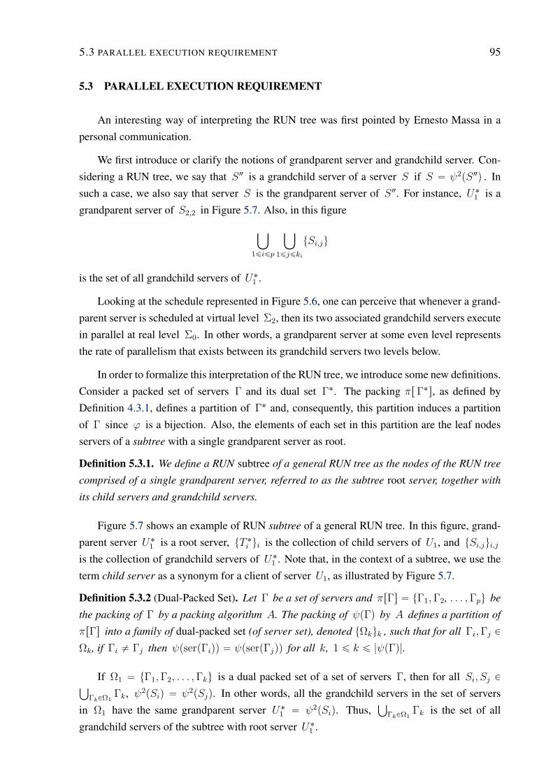
5.3 PARALLEL EXECUTION REQUIREMENT 95
5.3 PARALLEL EXECUTION REQUIREMENT
An interesting way of interpreting the RUN tree was first pointed by Ernesto Massa in a
personal communication.
We first introduce or clarify the notions of grandparent server and grandchild server. Con-
sidering a RUN tree, we say that S2 is a grandchild server of a server S if S “ ψ2pS2q . In
such a case, we also say that server S is the grandparent server of S2. For instance, U˚1
is a
grandparent server of S2,2 in Figure 5.7. Also, in this figure
ď
1ďiďp
ď
1ďjďki
tSi,ju
is the set of all grandchild servers of U˚1
.
Looking at the schedule represented in Figure 5.6, one can perceive that whenever a grand-
parent server is scheduled at virtual level Σ2, then its two associated grandchild servers execute
in parallel at real level Σ0. In other words, a grandparent server at some even level represents
the rate of parallelism that exists between its grandchild servers two levels below.
In order to formalize this interpretation of the RUN tree, we introduce some new definitions.
Consider a packed set of servers Γ and its dual set Γ˚. The packing πrΓ˚s, as defined by
Definition 4.3.1, defines a partition of Γ˚ and, consequently, this partition induces a partition
of Γ since ϕ is a bijection. Also, the elements of each set in this partition are the leaf nodes
servers of a subtree with a single grandparent server as root.
Definition 5.3.1. We define a RUN subtree of a general RUN tree as the nodes of the RUN tree
comprised of a single grandparent server, referred to as the subtree root server, together with
its child servers and grandchild servers.
Figure 5.7 shows an example of RUN subtree of a general RUN tree. In this figure, grand-
parent server U˚1
is a root server, tT ˚i ui is the collection of child servers of U1, and tSi,jui,j
is the collection of grandchild servers of U˚1
. Note that, in the context of a subtree, we use the
term child server as a synonym for a client of server U1, as illustrated by Figure 5.7.
Definition 5.3.2 (Dual-Packed Set). Let Γ be a set of servers and πrΓs “ tΓ1,Γ2, . . . ,Γpu be
the packing of Γ by a packing algorithm A. The packing of ψpΓq by A defines a partition of
πrΓs into a family of dual-packed set (of server set), denoted tΩkuk , such that for all Γi,Γj P
Ωk, if Γi ‰ Γj then ψpserpΓiqq “ ψpserpΓjqq for all k, 1 ď k ď |ψpΓq|.
If Ω1 “ tΓ1,Γ2, . . . ,Γku is a dual packed set of a set of servers Γ, then for all Si, Sj PŤ
ΓkPΩ1Γk, ψ2pSiq “ ψ2pSjq. In other words, all the grandchild servers in the set of servers
in Ω1 have the same grandparent server U˚1
“ ψ2pSiq. Thus,Ť
ΓkPΩ1Γk is the set of all
grandchild servers of the subtree with root server U˚1
.
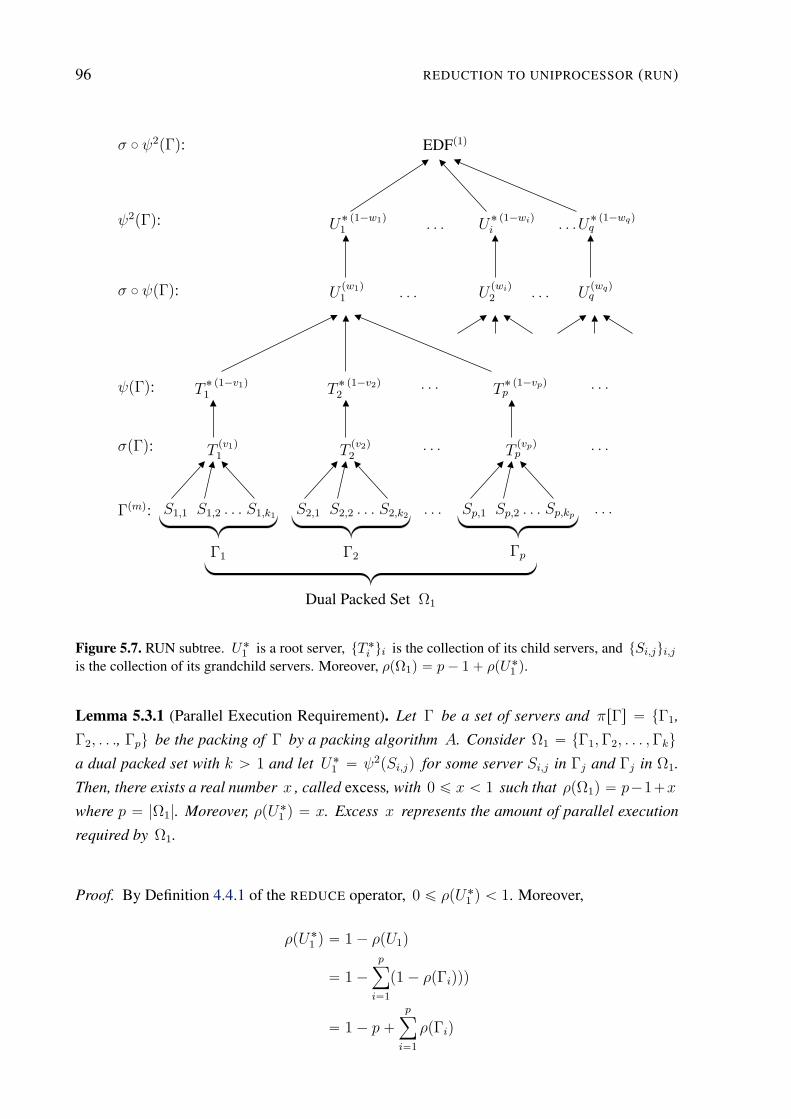
96 REDUCTION TO UNIPROCESSOR (RUN)
σ ˝ ψ2pΓq:
ψ2pΓq:
σ ˝ ψpΓq:
EDFp1q
U˚ p1´w1q1
. . . U˚ p1´wiqi . . .U
˚ p1´wqqq
Upw1q1
. . . Upwiq2
. . . Upwqqq
ψpΓq: T˚ p1´v1q1
T˚ p1´v2q2
. . . T˚ p1´vpqp
. . .
σpΓq: Tpv1q1
Tpv2q2
. . . Tpvpqp
. . .
Γpmq: S1,1 S1,2 . . . S1,k1 S2,1 S2,2 . . . S2,k2 . . . Sp,1 Sp,2 . . . Sp,kp . . .
Γ1 Γ2 Γp
Dual Packed Set Ω1
Figure 5.7. RUN subtree. U˚1
is a root server, tT ˚i ui is the collection of its child servers, and tSi,jui,j
is the collection of its grandchild servers. Moreover, ρpΩ1q “ p´ 1 ` ρpU˚1
q.
Lemma 5.3.1 (Parallel Execution Requirement). Let Γ be a set of servers and πrΓs “ tΓ1,
Γ2, . . ., Γpu be the packing of Γ by a packing algorithm A. Consider Ω1 “ tΓ1,Γ2, . . . ,Γku
a dual packed set with k ą 1 and let U˚1
“ ψ2pSi,jq for some server Si,j in Γj and Γj in Ω1.
Then, there exists a real number x , called excess, with 0 ď x ă 1 such that ρpΩ1q “ p´1`x
where p “ |Ω1|. Moreover, ρpU˚1
q “ x. Excess x represents the amount of parallel execution
required by Ω1.
Proof. By Definition 4.4.1 of the REDUCE operator, 0 ď ρpU˚1
q ă 1. Moreover,
ρpU˚1
q “ 1 ´ ρpU1q
“ 1 ´p
ÿ
i“1
p1 ´ ρpΓiqqq
“ 1 ´ p `p
ÿ
i“1
ρpΓiq
5.3 PARALLEL EXECUTION REQUIREMENT 97
ψ2pΓq: Up0.1q1
σ ˝ ψpΓq: U˚ p0.9q1
ϕ ˝ σpΓq: Tp0.3q1
Tp0.3q2
Tp0.3q3
σpΓq: T˚ p0.7q1
T˚ p0.7q2
T˚ p0.7q3
Γp2.1q: Sp0.7q1
Sp0.7q2
Sp0.7q3
Figure 5.8. A reduction subtree of the primal packed set of servers S1, S2 and S3. The notation Sµi
means that ρpSiq “ µ.
“ 1 ´ p ` ρpΩ1q
Hence, ρpΩ1q “ p ´ 1 ` x with x “ ρpU˚1
q.
It is important to emphasize that this latter equality means that a dual-packed set can be
scheduled on |Ωi| ´ 1 fully utilized processors and one partially utilized processor with rate x.
Also, note that if x “ 0, then the dual set of Ωi is a unit server and the scheduling problem
of Ωi can be solved, as shown by Theorem 4.2.1.
Let us consider a simple subtree example where root server U1 has only three grandchild
servers S1, S2 and S3, all of them with utilization 0.7, as illustrated in Figure 5.8. Observe
that, in this example, x “ 0.1 and that ρpΓq “ 2.1. Thus, two processors are “almost” enough to
schedule Γ. More precisely, the valid schedule of Γ requires two full processors and a fraction
0.1 of a third processor. In other words, two processors must be executing continuously two of
the three servers in Γ, and, when the third processor executes a server in Γ, for a fraction 0.1 of
its bandwidth, then the three servers in Γ are executing in parallel. As can be seen, 0.1 is the
computing requirement excess which prevents Γ to be feasible on two processors.
In this example, root server U˚1
has its rate precisely equal to excess 0.1 . Thus, U˚1
deals
with the amount of parallelism on three processors that the 3-server set Γ requires. This is
coherent with the RUN scheduling rules exposed earlier. Indeed, if U˚1
executes at time t, then
U1 does not by Rule 5.2.2. Hence, by Rule 5.2.1 at time t, T ˚1
, T ˚2
and T ˚3
, the U1 ’s clients,
do not execute. In turn, this implies, by Rule 5.2.2, that T1, T2 and T3 execute and finally, by
Rule 5.2.1, that S1, S2 and S3 execute in parallel on three processors at time t.
98 REDUCTION TO UNIPROCESSOR (RUN)
On the other hand, when U˚1
does not execute at time t, then U1 does. Hence, one of the
three servers T ˚1
, T ˚2
and T ˚3
executes whereas the two others do not. Assume for instance that
T ˚2
is the server with earliest deadline that executes at time t . Hence, T ˚1
and T ˚3
do not, and,
as a consequence, both T1 and S1 , and T3 and S3 execute at time t while T2 and S2 do not.
Summarizing, if Ω1 “ tΓ1,Γ2, . . . ,Γpu is a dual packed set of accumulated rate p´ 1`x
with 0 ď x ă 1, then, for any Si P Γj with Γj P Ω1, the grandparent server U˚1
“ ψ2pSiq of
Si has rate x, and whenever U˚1
executes, all servers serpΓjq in Ω1 execute on p processors
in parallel. Otherwise, when U˚1
does not execute, then p´ 1 servers in Ω1 execute on p´ 1
processors.
Also, the dual level ψpΩ1q guarantees the correct exclusion between executions of the p
servers in Ω1 while they are scheduled on p ´ 1 processors.
In appendix C, we will see how the decomposition of a general RUN tree into distinct
subtrees can possibly be used to develop a RUN-based solution for the sporadic task model
with implicit deadlines.
5.4 CONCLUSION
In this chapter, we have enunciated and explained the on-line scheduling rules used by the
RUN algorithm once computed the off-line reduction tree of a set of tasks.
Although the RUN tree incurs some complexity in the overall algorithm, it is computed
off-line. The on-line scheduling decisions use the previously computed RUN tree but follows
straightforward rules.
Further, an alternative interpretation of the RUN tree, based on its decomposition in distinct
subtrees, has been presented. More precisely, we have shown that in each subtree, comprised of
a grandparent root server, its child and grandchild servers, the parallel execution requirements
existing at the grandchild server level strictly corresponds to the executions of the root server.
In the next chapter, the whole RUN scheduling framework will be evaluated by simulation.
Chapter
6The number of reduction levels in a RUN tree is a logarithmic function of the total number of primal tasks. As
a consequence, RUN significantly outperforms existing optimal algorithms with an upper bound of Oplogmq
average preemptions per job on m processors ( ď 3 per job in all of our simulated task sets).
ASSESSMENT
6.1 INTRODUCTION
Now that we have completely and precisely described the reduction to uniprocessor real-
time scheduling algorithm, we establish in this chapter results on the number of preemption and
migration per job. Also, we characterize the complexity of the RUN algorithm.
As previously stated, for some particular task system, one or more iterations of the DUAL
and PACK operations may be needed in order to reach a set of unit servers. Hence, the complex-
ity of RUN depends upon the number m of identical processors, the total number n of tasks of
the primal set to be scheduled and the number of reduction levels required by this task system.
However, as will be seen in this chapter, the number of reduction levels is a logarithmic
function of the total number of primal tasks. As a consequence, we establish an upper bound
on the average number of preemptions per job, which is a function of m and n .
Structure of the chapter
Section 6.2 deals with implementation details, describing how the bin-packing procedure
can take profit of some slack in the task system. Then, the overall complexity of the RUN
scheme is shown in Section 6.3.
The theoretical results presented in Section 6.4 and 6.5 were originally proposed by Greg
Levin in (REGNIER et al., 2011). For the sake of completeness, we include these results in the
dissertation.
99
100 ASSESSMENT
In Section 6.6, the RUN algorithm is compared with many other optimal scheduling algo-
rithms through intensive simulations, using randomly generated tasks sets.
6.2 RUN IMPLEMENTATION
At the first reduction level, we have m bins, i.e., processors, each of which has size, i.e.,
bandwidth, equal to one. On the other hand, we have a real-time set of n primal tasks that must
be packed into at least m servers of rate less than or equal to one according to some bin-packing
policy with property enunciated in Definition 4.3.1. Thereafter, at each supplementary level of
reduction needed, child servers are packed into parent servers to be scheduled on less virtual
processors than what would be needed at the child level.
In order to pack tasks at the primal level as well as at each reduction level, our implemen-
tation of RUN uses the worst-fit bin-packing heuristic, which runs in Opk log kq time where k
is the number of tasks to be packed.
Also, our reduction procedure isolates off proper subsystems as soon as unit servers are
found. In other words, each unit server and its descendants make an isolated scheduling reduc-
tion tree in which servers and primal tasks are scheduled by the RUN algorithm applied to this
isolated subsystem, independently from all other subsystems required to schedule the complete
primal task set.
As for the job-to-processor assignment algorithm, at each scheduler invocation, once the
set of m running tasks is determined by the RUN algorithm (as in Figure 5.5), we use a simple
greedy assignment scheme. In three passes through these m tasks, we first leave executing
tasks on their current processors; second, we assign idle tasks to their last-used processor, when
available, to avoid unnecessary migrations; and third, we assign remaining tasks to the remain-
ing free processors arbitrarily.
Recall from Chapter 4 that duality is only defined for task sets with 100% utilization. For
the sake of simplicity, we have assumed in Chapter 3 a fully-utilized system of m identical
processors. However, when a primal task set does not fully-utilizes the m processors in the
system, one can define dummy tasks to fill in the difference when needed. In such a case, it is
possible to take advantage of the possible slack in the task system to improve performance.
To this end, we introduce the slack packing heuristic, as originally formalized by Greg
Levin in (REGNIER et al., 2011), to distribute a task system’s slack (defined as m ´ ρpT q)
among the aggregated servers at the end of the initial PACK step. Servers are filled to become
unit servers, and then isolated from the system. The result is that some or all processors are
assigned only non-migrating tasks and behave as they would in a partitioned schedule.
For example, suppose that the task set from Figure 5.5 runs on four processors instead
6.3 REDUCTION COMPLEXITY 101
of three. The initial PACK can only place one 0.6 utilization task per server. From the 1
unit of slack provided by our fourth processor, we create a dummy task Sd1
with ρpSd1q “
0.4 (and arbitrarily large deadline), pack it with S1 to get a unit server and give it its own
processor. Similarly, S2 also gets a dedicated processor. Since S1 and S2 never need preempt
or migrate, the schedule is more efficient. With 5 processors, this approach yields a fully
partitioned system, where each task has its own processor. With low enough utilization, the first
PACK usually results in m or fewer servers. In these cases, slack packing gracefully reduces
RUN to Partitioned EDF.
It is important to note here that RUN does not rely on task synchronization like in previous
optimal approaches based on Pfair. As a consequence, RUN is more compatible with symmetric
multiprocessor (SMP) architectures than previous approaches since RUN generates less bus
contention than Pfair approaches. Indeed, the quantum-based approach of Pfair implies that
tasks may need to reload data into local caches at the start of each quantum, resulting in a
period of increased bus traffic (HOLMAN, 2004). Since, under Pfair scheduling, quanta begin
synchronously on all processors, the resulting bus traffic bursts generate a heavy bus contention
at the start of each quantum. However, no such synchronization occurs under RUN scheduling,
resulting in less bus contention than Pfair scheduling approaches.
6.3 REDUCTION COMPLEXITY
We now observe that the time complexity of a reduction procedure is polynomial and is
dominated by the PACK operation. However, as there is no specific requirement on the (off-line)
reduction procedure, any polynomial-time heuristic suffices. There are, for example, linear
and log-linear time packing algorithms available (COFFMAN JR. et al., 1997; HOCHBAUM,
1997).
The following lemma establishes an upper bound on the number of servers obtained by
packing an arbitrary number of servers.
Lemma 6.3.1. Let Γ be a set of servers. Then, |σpΓq| ă 2 ρpΓq.
Proof. Let q “ |σpΓq| and ui “ ρpSiq for Si P σpΓq. Since σpΓq is packed, there exists
at most one server in σpΓq, as stated by Lemma 4.3.1, say Sq, such that uq ă 12. All other
servers have utilization greater that 12. Thus,
q´2ÿ
i“1
ui ąpq ´ 2q
2.
102 ASSESSMENT
As uq´1 ` uq ą 1, it follows that
qÿ
i“1
ui “ ρpΓq ą n2.
Theorem 6.3.1 (Reduction Complexity). RUN’s off-line generation of a reduction sequence for
n tasks on m processors requires Oplogmq reduction steps and Opfpnqq time, where fpnq
is the time needed to pack n tasks.
Proof. Let tψiuiďp be a reduction sequence on T , where p is the terminal level described in
Theorem 4.4.1. Lemma 4.4.1 shows that a REDUCE operation, at worst, reduces the number of
servers by about half, so p “ Oplog nq.
Also, since T is a full utilization task set, ρpT q “ m. If we let n1 “ |σpT q|, Lemma
6.3.1 tells us that m “ ρpT q “ ρpσpT qq ą n12. But as σpT q is just the one initial packing, it
follows that p also is Oplog n1q, and hence Oplogmq.
Finally, since constructing the dual of a system primarily requires computing n dual rates,
a single REDUCE operation requires Opfpnq ` nq time. Hence, the time needed to perform
the entire reduction sequence is described by T pnq ď T pn2q ` Opfpnq ` nq, which gives
T pnq “ Opfpnqq.
6.4 ON-LINE COMPLEXITY
As already seen, the RUN reduction is computed off-line, i.e., during design time. Thus,
the on-line complexity of RUN can be estimated using the off-line computed RUN tree and
calculating the time and complexity introduced by on-line scheduling according to Rules 3.4.1
and 4.2.1. In order to do so, we consider a time window during which j jobs are released by
the system of n tasks to be scheduled.
Theorem 6.4.1 (On-line Complexity). Each scheduler invocation of RUN takes Opnq time, for
a total of Opjn logmq scheduling overhead during any time interval when n tasks releasing a
total of j jobs are scheduled on m processors.
Proof. First, let’s count the nodes in the RUN tree. In practice, a primal/dual pair comprised
by a server S and its dual server S˚ may be implemented as a single node. Also, there are n
leaves at the primal level of the RUN tree, and as many as n servers in σpT q. Above that, each
level of the RUN tree has at most (approximately) half as many nodes as the preceding level.
This gives us an approximate node bound of n`n`n2`n4` . . . “ n`np1p1´12qq “ 3n
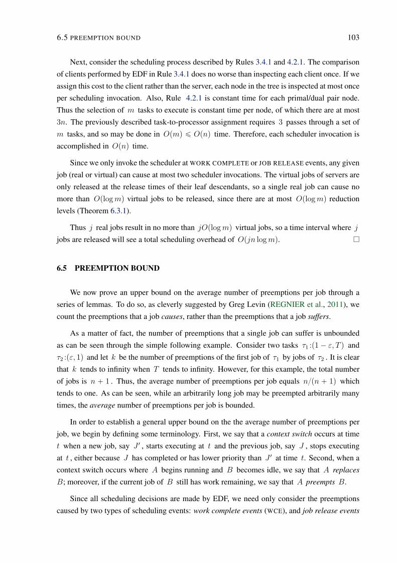
6.5 PREEMPTION BOUND 103
Next, consider the scheduling process described by Rules 3.4.1 and 4.2.1. The comparison
of clients performed by EDF in Rule 3.4.1 does no worse than inspecting each client once. If we
assign this cost to the client rather than the server, each node in the tree is inspected at most once
per scheduling invocation. Also, Rule 4.2.1 is constant time for each primal/dual pair node.
Thus the selection of m tasks to execute is constant time per node, of which there are at most
3n. The previously described task-to-processor assignment requires 3 passes through a set of
m tasks, and so may be done in Opmq ď Opnq time. Therefore, each scheduler invocation is
accomplished in Opnq time.
Since we only invoke the scheduler at WORK COMPLETE or JOB RELEASE events, any given
job (real or virtual) can cause at most two scheduler invocations. The virtual jobs of servers are
only released at the release times of their leaf descendants, so a single real job can cause no
more than Oplogmq virtual jobs to be released, since there are at most Oplogmq reduction
levels (Theorem 6.3.1).
Thus j real jobs result in no more than jOplogmq virtual jobs, so a time interval where j
jobs are released will see a total scheduling overhead of Opjn logmq.
6.5 PREEMPTION BOUND
We now prove an upper bound on the average number of preemptions per job through a
series of lemmas. To do so, as cleverly suggested by Greg Levin (REGNIER et al., 2011), we
count the preemptions that a job causes, rather than the preemptions that a job suffers.
As a matter of fact, the number of preemptions that a single job can suffer is unbounded
as can be seen through the simple following example. Consider two tasks τ1 :p1 ´ ε, T q and
τ2 :pε, 1q and let k be the number of preemptions of the first job of τ1 by jobs of τ2 . It is clear
that k tends to infinity when T tends to infinity. However, for this example, the total number
of jobs is n ` 1 . Thus, the average number of preemptions per job equals npn ` 1q which
tends to one. As can be seen, while an arbitrarily long job may be preempted arbitrarily many
times, the average number of preemptions per job is bounded.
In order to establish a general upper bound on the the average number of preemptions per
job, we begin by defining some terminology. First, we say that a context switch occurs at time
t when a new job, say J 1 , starts executing at t and the previous job, say J , stops executing
at t , either because J has completed or has lower priority than J 1 at time t. Second, when a
context switch occurs where A begins running and B becomes idle, we say that A replaces
B; moreover, if the current job of B still has work remaining, we say that A preempts B.
Since all scheduling decisions are made by EDF, we need only consider the preemptions
caused by two types of scheduling events: work complete events (WCE), and job release events
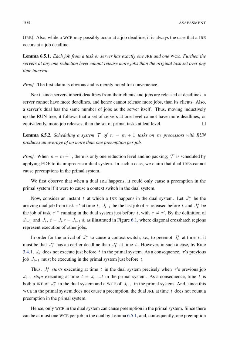
104 ASSESSMENT
(JRE). Also, while a WCE may possibly occur at a job deadline, it is always the case that a JRE
occurs at a job deadline.
Lemma 6.5.1. Each job from a task or server has exactly one JRE and one WCE. Further, the
servers at any one reduction level cannot release more jobs than the original task set over any
time interval.
Proof. The first claim is obvious and is merely noted for convenience.
Next, since servers inherit deadlines from their clients and jobs are released at deadlines, a
server cannot have more deadlines, and hence cannot release more jobs, than its clients. Also,
a server’s dual has the same number of jobs as the server itself. Thus, moving inductively
up the RUN tree, it follows that a set of servers at one level cannot have more deadlines, or
equivalently, more job releases, than the set of primal tasks at leaf level.
Lemma 6.5.2. Scheduling a system T of n “ m ` 1 tasks on m processors with RUN
produces an average of no more than one preemption per job.
Proof. When n “ m` 1, there is only one reduction level and no packing; T is scheduled by
applying EDF to its uniprocessor dual system. In such a case, we claim that dual JREs cannot
cause preemptions in the primal system.
We first observe that when a dual JRE happens, it could only cause a preemption in the
primal system if it were to cause a context switch in the dual system.
Now, consider an instant t at which a JRE happens in the dual system. Let J˚i be the
arriving dual job from task τ˚ at time t , Ji´1 be the last job of τ released before t and J˚k be
the job of task τ 1 ˚ running in the dual system just before t, with τ ‰ τ 1. By the definition of
Ji´1 and Ji , t “ Ji.r “ Ji´1.d, as illustrated in Figure 6.1, where diagonal crosshatch regions
represent execution of other jobs.
In order for the arrival of J˚i to cause a context switch, i.e., to preempt J˚
k at time t , it
must be that J˚i has an earlier deadline than J˚
k at time t . However, in such a case, by Rule
3.4.1, Jk does not execute just before t in the primal system. As a consequence, τ ’s previous
job Ji´1 must be executing in the primal system just before t.
Thus, J˚i starts executing at time t in the dual system precisely when τ ’s previous job
Ji´1 stops executing at time t “ Ji´1.d in the primal system. As a consequence, time t is
both a JRE of J˚i in the dual system and a WCE of Ji´1 in the primal system. And, since this
WCE in the primal system does not cause a preemption, the dual JRE at time t does not count a
preemption in the primal system.
Hence, only WCE in the dual system can cause preemption in the primal system. Since there
can be at most one WCE per job in the dual by Lemma 6.5.1, and, consequently, one preemption
6.5 PREEMPTION BOUND 105
Dual SystemJ˚k
J˚i´1.d
t “ J˚i .r
J˚i
J˚i .d
Primal System
Ji´1.r
Ji´1
Ji´1.d
t “ Ji.r
Ji
Ji.d
Jk
Figure 6.1. In the dual, the arrival of J˚i preempts J˚
k . The matching primal event is just the previousjob Ji´1 finishing its work at its deadline, and is not a preemption.
in the primal, we conclude that there can be only one preemption in the primal system for each
job released by a task in T , as desired.
Lemma 6.5.3. A context switch at any level of the RUN tree causes exactly one context switch
between two primal leaf tasks in T .
Proof. We proceed by induction on the number of levels, showing that a context switch at any
level of the RUN tree causes exactly one context switch in the next level below (less reduced
than) it.
Consider some tree level where a context switch occurs at time t and suppose we have a pair
of client nodes (not necessarily of the same server parent) C`,0 and C´,1, where C`,0 replaces
C´,1. We use the ` and ´ signals to indicate that C`,0 preempts C´,1 . Moreover, indexes
0 and 1 allow us to distinguishes between clients of a same server. All other jobs’ “running”
statuses at this level remain unchanged at time t.
Now, let S`,0 and S´,1 be the dual children of C`,0 and C´,1 in the RUN tree, respectively
(i.e., C`,0 “ S˚`,0 and C´,1 “ S˚
´,1). By the dual scheduling Rule 4.2.1, it must be that S´,1
replaces S`,0 (see Figure 6.2 for node relationships).
Now, when server S`,0 was running, it was executing exactly one of its client children, say
C`,0,1, and when S`,0 gets switched off, so does C`,0,1. Similarly, when S´,0 was off, none
of its clients were running, and when it gets switched on, exactly one of its clients, say C´,1,0,
begins to execute.
Also, just as the context switch at the higher (more reduced) level only effects the two
servers C`,0 and C´,1, so too are these two clients C`,0,1 and C´,1,0 the only clients at this
106 ASSESSMENT
Not running before or after J.r
Running before and after J.r
Starts running at time J.r
Stops running at time J.r
A replaces BA B
Dual nodes˚
S
C`,0 C´,1
(i)˚
S`,0
˚
S´,0
C`,0,0
˚
S`,0,0
C`,0,1
˚
S`,0,1
C´,1,0
˚
S´,1,0
(ii)
C`,0,0,0 C`,0,0,1
(iv)
C`,0,1,0 C`,0,1,1 C´,1,1,0 C´,1,1,1
(iii)τ
Figure 6.2. Two Preemptions from one job release In this 3-level part of a RUN tree, only relevantnodes are shown. A job release by τ corresponds to a job release and context switch at the top level(i), which propagates down to the right of the tree (ii, iii). That same job release by τ can cause it topreempt (iv) another client C`,0,0,1 of its parent server S`,0,0.
lower level affected by this operation; thus, C´,1,0 must be replacing C`,0,1. So here we see
that a context switch at one client level of the RUN tree causes only a single context switch at
the next lower client level of the tree (in terms of Figure 6.2, (i) causes (ii)).
This one context switch propagates down to the leaves, so inductively, a context switch
anywhere in the RUN tree causes exactly one context switch in T .
Lemma 6.5.4. If RUN requires p reduction levels for a task set T , then any JRE by a task
τ P T can cause at most rpp ` 1q2s preemptions in T .
Proof. Suppose task τ releases job J at time J.r. This causes a job release at each ancestor
server node above τ in the RUN tree (i.e., on the path from leaf τ to the root). We will
use Figure 6.2 for reference. Note that this figure represents only the relevant nodes for our
discussion of a particular subtree, as stated in Definition 5.3.1, of a general RUN tree.
Let S be the highest ancestor server of τ in the RUN tree (S may be the root of the RUN
tree) for which this JRE causes a context switch among its clients. As a consequence, some
client of S , say C`,0, has a job arrive with an earlier deadline than the currently executing
client, say C´,1, so C`,0 preempts C´,1. As described in the proof of Lemma 6.5.3, C´,1’s
dual S´,1 replaces C`,0’s dual S`,0, and this context switch propagates down to a context
switch between two tasks in T , i.e., preemption (iii) in Figure 6.2.
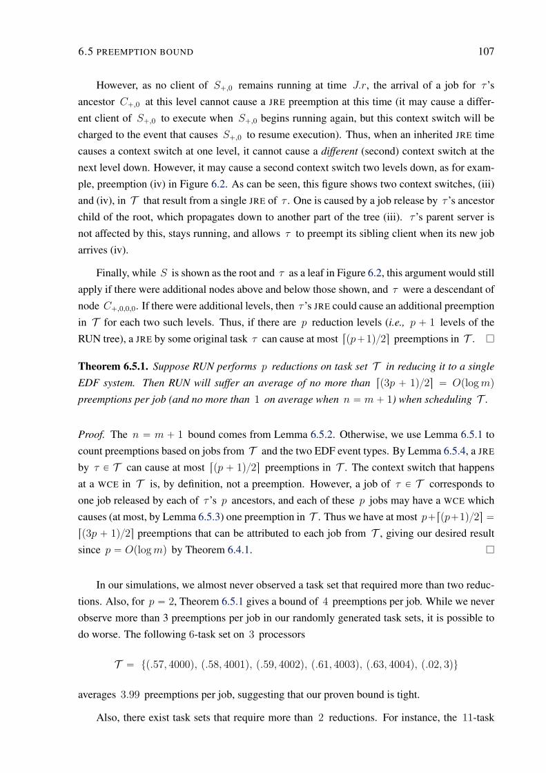
6.5 PREEMPTION BOUND 107
However, as no client of S`,0 remains running at time J.r, the arrival of a job for τ ’s
ancestor C`,0 at this level cannot cause a JRE preemption at this time (it may cause a differ-
ent client of S`,0 to execute when S`,0 begins running again, but this context switch will be
charged to the event that causes S`,0 to resume execution). Thus, when an inherited JRE time
causes a context switch at one level, it cannot cause a different (second) context switch at the
next level down. However, it may cause a second context switch two levels down, as for exam-
ple, preemption (iv) in Figure 6.2. As can be seen, this figure shows two context switches, (iii)
and (iv), in T that result from a single JRE of τ . One is caused by a job release by τ ’s ancestor
child of the root, which propagates down to another part of the tree (iii). τ ’s parent server is
not affected by this, stays running, and allows τ to preempt its sibling client when its new job
arrives (iv).
Finally, while S is shown as the root and τ as a leaf in Figure 6.2, this argument would still
apply if there were additional nodes above and below those shown, and τ were a descendant of
node C`,0,0,0. If there were additional levels, then τ ’s JRE could cause an additional preemption
in T for each two such levels. Thus, if there are p reduction levels (i.e., p ` 1 levels of the
RUN tree), a JRE by some original task τ can cause at most rpp`1q2s preemptions in T .
Theorem 6.5.1. Suppose RUN performs p reductions on task set T in reducing it to a single
EDF system. Then RUN will suffer an average of no more than rp3p ` 1q2s “ Oplogmq
preemptions per job (and no more than 1 on average when n “ m ` 1) when scheduling T .
Proof. The n “ m ` 1 bound comes from Lemma 6.5.2. Otherwise, we use Lemma 6.5.1 to
count preemptions based on jobs from T and the two EDF event types. By Lemma 6.5.4, a JRE
by τ P T can cause at most rpp ` 1q2s preemptions in T . The context switch that happens
at a WCE in T is, by definition, not a preemption. However, a job of τ P T corresponds to
one job released by each of τ ’s p ancestors, and each of these p jobs may have a WCE which
causes (at most, by Lemma 6.5.3) one preemption in T . Thus we have at most p`rpp`1q2s “
rp3p ` 1q2s preemptions that can be attributed to each job from T , giving our desired result
since p “ Oplogmq by Theorem 6.4.1.
In our simulations, we almost never observed a task set that required more than two reduc-
tions. Also, for p “ 2, Theorem 6.5.1 gives a bound of 4 preemptions per job. While we never
observe more than 3 preemptions per job in our randomly generated task sets, it is possible to
do worse. The following 6-task set on 3 processors
T “ tp.57, 4000q, p.58, 4001q, p.59, 4002q, p.61, 4003q, p.63, 4004q, p.02, 3qu
averages 3.99 preemptions per job, suggesting that our proven bound is tight.
Also, there exist task sets that require more than 2 reductions. For instance, the 11-task
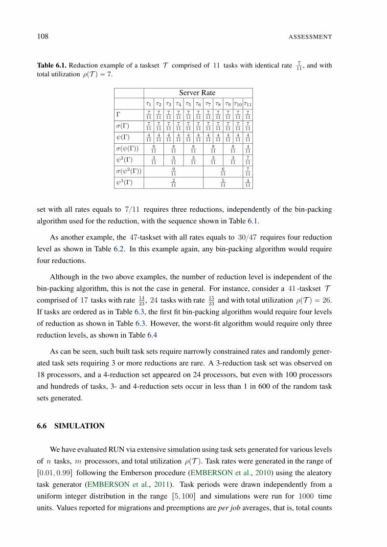
108 ASSESSMENT
Table 6.1. Reduction example of a taskset T comprised of 11 tasks with identical rate 7
11, and with
total utilization ρpT q “ 7.
Server Rateτ1 τ2 τ3 τ4 τ5 τ6 τ7 τ8 τ9 τ10 τ11
Γ 7
11
7
11
7
11
7
11
7
11
7
11
7
11
7
11
7
11
7
11
7
11
σpΓq 7
11
7
11
7
11
7
11
7
11
7
11
7
11
7
11
7
11
7
11
7
11
ψpΓq 4
11
4
11
4
11
4
11
4
11
4
11
4
11
4
11
4
11
4
11
4
11
σpψpΓqq 8
11
8
11
8
11
8
11
8
11
4
11
ψ2pΓq 3
11
3
11
3
11
3
11
3
11
7
11
σpψ2pΓqq 9
11
6
11
7
11
ψ3pΓq 2
11
5
11
4
11
set with all rates equals to 711 requires three reductions, independently of the bin-packing
algorithm used for the reduction, with the sequence shown in Table 6.1.
As another example, the 47-taskset with all rates equals to 3047 requires four reduction
level as shown in Table 6.2. In this example again, any bin-packing algorithm would require
four reductions.
Although in the two above examples, the number of reduction level is independent of the
bin-packing algorithm, this is not the case in general. For instance, consider a 41 -taskset T
comprised of 17 tasks with rate 14
23, 24 tasks with rate 15
23and with total utilization ρpT q “ 26.
If tasks are ordered as in Table 6.3, the first fit bin-packing algorithm would require four levels
of reduction as shown in Table 6.3. However, the worst-fit algorithm would require only three
reduction levels, as shown in Table 6.4
As can be seen, such built task sets require narrowly constrained rates and randomly gener-
ated task sets requiring 3 or more reductions are rare. A 3-reduction task set was observed on
18 processors, and a 4-reduction set appeared on 24 processors, but even with 100 processors
and hundreds of tasks, 3- and 4-reduction sets occur in less than 1 in 600 of the random task
sets generated.
6.6 SIMULATION
We have evaluated RUN via extensive simulation using task sets generated for various levels
of n tasks, m processors, and total utilization ρpT q. Task rates were generated in the range of
r0.01, 0.99s following the Emberson procedure (EMBERSON et al., 2010) using the aleatory
task generator (EMBERSON et al., 2011). Task periods were drawn independently from a
uniform integer distribution in the range r5, 100s and simulations were run for 1000 time
units. Values reported for migrations and preemptions are per job averages, that is, total counts
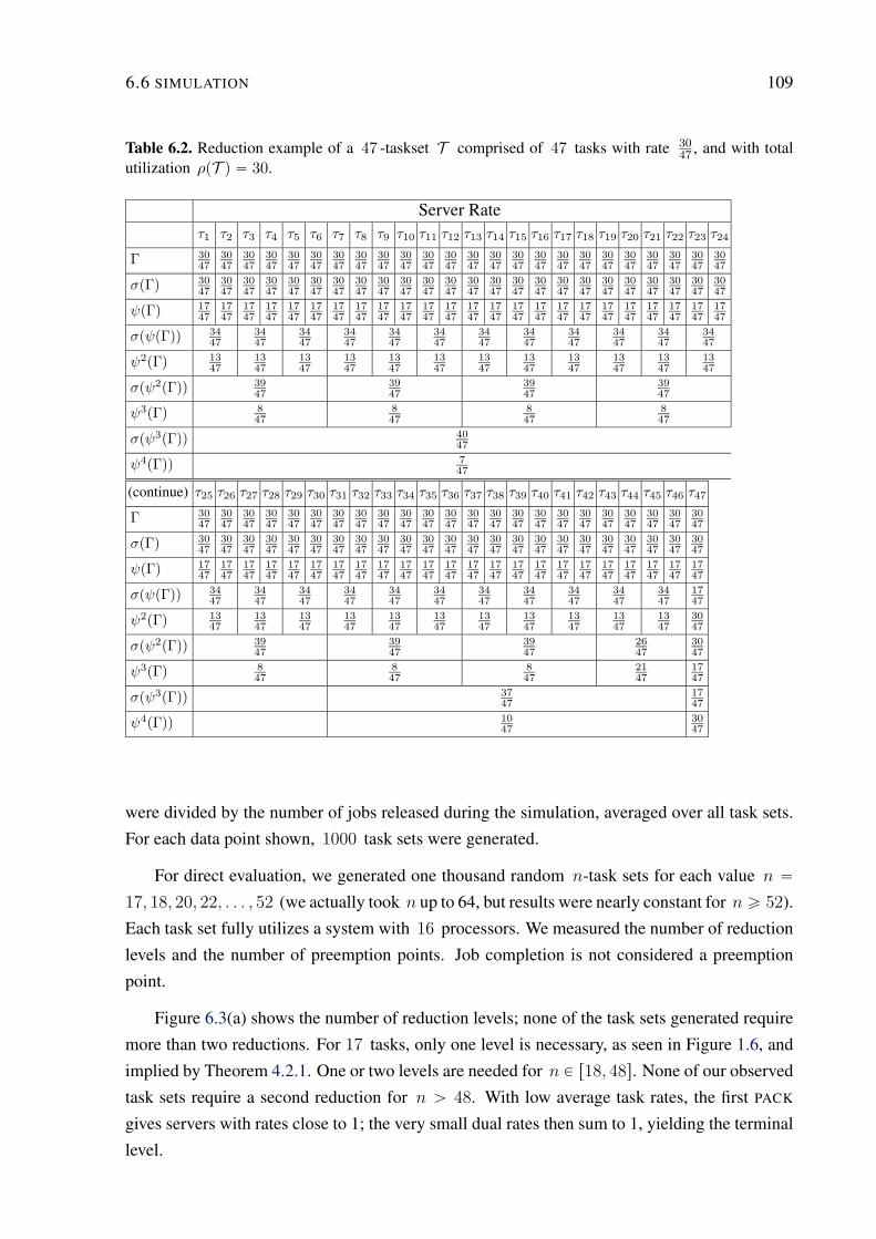
6.6 SIMULATION 109
Table 6.2. Reduction example of a 47 -taskset T comprised of 47 tasks with rate 30
47, and with total
utilization ρpT q “ 30.
Server Rateτ1 τ2 τ3 τ4 τ5 τ6 τ7 τ8 τ9 τ10 τ11 τ12 τ13 τ14 τ15 τ16 τ17 τ18 τ19 τ20 τ21 τ22 τ23 τ24
Γ 30
47
30
47
30
47
30
47
30
47
30
47
30
47
30
47
30
47
30
47
30
47
30
47
30
47
30
47
30
47
30
47
30
47
30
47
30
47
30
47
30
47
30
47
30
47
30
47
σpΓq 30
47
30
47
30
47
30
47
30
47
30
47
30
47
30
47
30
47
30
47
30
47
30
47
30
47
30
47
30
47
30
47
30
47
30
47
30
47
30
47
30
47
30
47
30
47
30
47
ψpΓq 17
47
17
47
17
47
17
47
17
47
17
47
17
47
17
47
17
47
17
47
17
47
17
47
17
47
17
47
17
47
17
47
17
47
17
47
17
47
17
47
17
47
17
47
17
47
17
47
σpψpΓqq 34
47
34
47
34
47
34
47
34
47
34
47
34
47
34
47
34
47
34
47
34
47
34
47
ψ2pΓq 13
47
13
47
13
47
13
47
13
47
13
47
13
47
13
47
13
47
13
47
13
47
13
47
σpψ2pΓqq 39
47
39
47
39
47
39
47
ψ3pΓq 8
47
8
47
8
47
8
47
σpψ3pΓqq 40
47
ψ4pΓqq 7
47
(continue) τ25 τ26 τ27 τ28 τ29 τ30 τ31 τ32 τ33 τ34 τ35 τ36 τ37 τ38 τ39 τ40 τ41 τ42 τ43 τ44 τ45 τ46 τ47
Γ 30
47
30
47
30
47
30
47
30
47
30
47
30
47
30
47
30
47
30
47
30
47
30
47
30
47
30
47
30
47
30
47
30
47
30
47
30
47
30
47
30
47
30
47
30
47
σpΓq 30
47
30
47
30
47
30
47
30
47
30
47
30
47
30
47
30
47
30
47
30
47
30
47
30
47
30
47
30
47
30
47
30
47
30
47
30
47
30
47
30
47
30
47
30
47
ψpΓq 17
47
17
47
17
47
17
47
17
47
17
47
17
47
17
47
17
47
17
47
17
47
17
47
17
47
17
47
17
47
17
47
17
47
17
47
17
47
17
47
17
47
17
47
17
47
σpψpΓqq 34
47
34
47
34
47
34
47
34
47
34
47
34
47
34
47
34
47
34
47
34
47
17
47
ψ2pΓq 13
47
13
47
13
47
13
47
13
47
13
47
13
47
13
47
13
47
13
47
13
47
30
47
σpψ2pΓqq 39
47
39
47
39
47
26
47
30
47
ψ3pΓq 8
47
8
47
8
47
21
47
17
47
σpψ3pΓqq 37
47
17
47
ψ4pΓqq 10
47
30
47
were divided by the number of jobs released during the simulation, averaged over all task sets.
For each data point shown, 1000 task sets were generated.
For direct evaluation, we generated one thousand random n-task sets for each value n “
17, 18, 20, 22, . . . , 52 (we actually took n up to 64, but results were nearly constant for n ě 52).
Each task set fully utilizes a system with 16 processors. We measured the number of reduction
levels and the number of preemption points. Job completion is not considered a preemption
point.
Figure 6.3(a) shows the number of reduction levels; none of the task sets generated require
more than two reductions. For 17 tasks, only one level is necessary, as seen in Figure 1.6, and
implied by Theorem 4.2.1. One or two levels are needed for n P r18, 48s. None of our observed
task sets require a second reduction for n ą 48. With low average task rates, the first PACK
gives servers with rates close to 1; the very small dual rates then sum to 1, yielding the terminal
level.
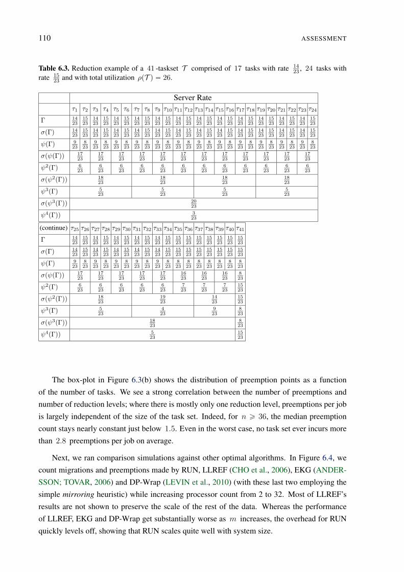
110 ASSESSMENT
Table 6.3. Reduction example of a 41 -taskset T comprised of 17 tasks with rate 14
23, 24 tasks with
rate 15
23and with total utilization ρpT q “ 26.
Server Rateτ1 τ2 τ3 τ4 τ5 τ6 τ7 τ8 τ9 τ10 τ11 τ12 τ13 τ14 τ15 τ16 τ17 τ18 τ19 τ20 τ21 τ22 τ23 τ24
Γ 14
23
15
23
14
23
15
23
14
23
15
23
14
23
15
23
14
23
15
23
14
23
15
23
14
23
15
23
14
23
15
23
14
23
15
23
14
23
15
23
14
23
15
23
14
23
15
23
σpΓq 14
23
15
23
14
23
15
23
14
23
15
23
14
23
15
23
14
23
15
23
14
23
15
23
14
23
15
23
14
23
15
23
14
23
15
23
14
23
15
23
14
23
15
23
14
23
15
23
ψpΓq 9
23
8
23
9
23
8
23
9
23
8
23
9
23
8
23
9
23
8
23
9
23
8
23
9
23
8
23
9
23
8
23
9
23
8
23
9
23
8
23
9
23
8
23
9
23
8
23
σpψpΓqq 17
23
17
23
17
23
17
23
17
23
17
23
17
23
17
23
17
23
17
23
17
23
17
23
ψ2pΓq 6
23
6
23
6
23
6
23
6
23
6
23
6
23
6
23
6
23
6
23
6
23
6
23
σpψ2pΓqq 18
23
18
23
18
23
18
23
ψ3pΓq 5
23
5
23
5
23
5
23
σpψ3pΓqq 20
23
ψ4pΓqq 3
23
(continue) τ25 τ26 τ27 τ28 τ29 τ30 τ31 τ32 τ33 τ34 τ35 τ36 τ37 τ38 τ39 τ40 τ41
Γ 14
23
15
23
14
23
15
23
14
23
15
23
14
23
15
23
14
23
15
23
15
23
15
23
15
23
15
23
15
23
15
23
15
23
σpΓq 14
23
15
23
14
23
15
23
14
23
15
23
14
23
15
23
14
23
15
23
15
23
15
23
15
23
15
23
15
23
15
23
15
23
ψpΓq 9
23
8
23
9
23
8
23
9
23
8
23
9
23
8
23
9
23
8
23
8
23
8
23
8
23
8
23
8
23
8
23
8
23
σpψpΓqq 17
23
17
23
17
23
17
23
17
23
16
23
16
23
16
23
8
23
ψ2pΓq 6
23
6
23
6
23
6
23
6
23
7
23
7
23
7
23
15
23
σpψ2pΓqq 18
23
19
23
14
23
15
23
ψ3pΓq 5
23
4
23
9
23
8
23
σpψ3pΓqq 18
23
8
23
ψ4pΓqq 5
23
15
23
The box-plot in Figure 6.3(b) shows the distribution of preemption points as a function
of the number of tasks. We see a strong correlation between the number of preemptions and
number of reduction levels; where there is mostly only one reduction level, preemptions per job
is largely independent of the size of the task set. Indeed, for n ě 36, the median preemption
count stays nearly constant just below 1.5. Even in the worst case, no task set ever incurs more
than 2.8 preemptions per job on average.
Next, we ran comparison simulations against other optimal algorithms. In Figure 6.4, we
count migrations and preemptions made by RUN, LLREF (CHO et al., 2006), EKG (ANDER-
SSON; TOVAR, 2006) and DP-Wrap (LEVIN et al., 2010) (with these last two employing the
simple mirroring heuristic) while increasing processor count from 2 to 32. Most of LLREF’s
results are not shown to preserve the scale of the rest of the data. Whereas the performance
of LLREF, EKG and DP-Wrap get substantially worse as m increases, the overhead for RUN
quickly levels off, showing that RUN scales quite well with system size.
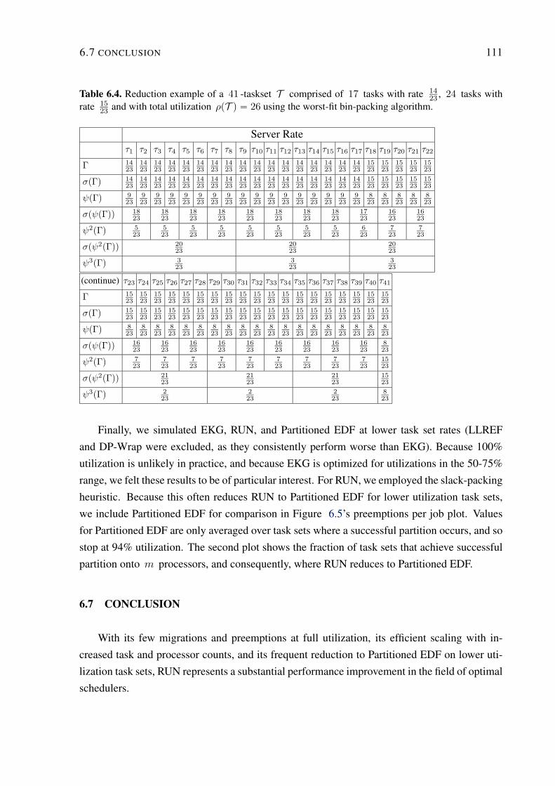
6.7 CONCLUSION 111
Table 6.4. Reduction example of a 41 -taskset T comprised of 17 tasks with rate 14
23, 24 tasks with
rate 15
23and with total utilization ρpT q “ 26 using the worst-fit bin-packing algorithm.
Server Rateτ1 τ2 τ3 τ4 τ5 τ6 τ7 τ8 τ9 τ10 τ11 τ12 τ13 τ14 τ15 τ16 τ17 τ18 τ19 τ20 τ21 τ22
Γ 14
23
14
23
14
23
14
23
14
23
14
23
14
23
14
23
14
23
14
23
14
23
14
23
14
23
14
23
14
23
14
23
14
23
15
23
15
23
15
23
15
23
15
23
σpΓq 14
23
14
23
14
23
14
23
14
23
14
23
14
23
14
23
14
23
14
23
14
23
14
23
14
23
14
23
14
23
14
23
14
23
15
23
15
23
15
23
15
23
15
23
ψpΓq 9
23
9
23
9
23
9
23
9
23
9
23
9
23
9
23
9
23
9
23
9
23
9
23
9
23
9
23
9
23
9
23
9
23
8
23
8
23
8
23
8
23
8
23
σpψpΓqq 18
23
18
23
18
23
18
23
18
23
18
23
18
23
18
23
17
23
16
23
16
23
ψ2pΓq 5
23
5
23
5
23
5
23
5
23
5
23
5
23
5
23
6
23
7
23
7
23
σpψ2pΓqq 20
23
20
23
20
23
ψ3pΓq 3
23
3
23
3
23
(continue) τ23 τ24 τ25 τ26 τ27 τ28 τ29 τ30 τ31 τ32 τ33 τ34 τ35 τ36 τ37 τ38 τ39 τ40 τ41
Γ 15
23
15
23
15
23
15
23
15
23
15
23
15
23
15
23
15
23
15
23
15
23
15
23
15
23
15
23
15
23
15
23
15
23
15
23
15
23
σpΓq 15
23
15
23
15
23
15
23
15
23
15
23
15
23
15
23
15
23
15
23
15
23
15
23
15
23
15
23
15
23
15
23
15
23
15
23
15
23
ψpΓq 8
23
8
23
8
23
8
23
8
23
8
23
8
23
8
23
8
23
8
23
8
23
8
23
8
23
8
23
8
23
8
23
8
23
8
23
8
23
σpψpΓqq 16
23
16
23
16
23
16
23
16
23
16
23
16
23
16
23
16
23
8
23
ψ2pΓq 7
23
7
23
7
23
7
23
7
23
7
23
7
23
7
23
7
23
15
23
σpψ2pΓqq 21
23
21
23
21
23
15
23
ψ3pΓq 2
23
2
23
2
23
8
23
Finally, we simulated EKG, RUN, and Partitioned EDF at lower task set rates (LLREF
and DP-Wrap were excluded, as they consistently perform worse than EKG). Because 100%
utilization is unlikely in practice, and because EKG is optimized for utilizations in the 50-75%
range, we felt these results to be of particular interest. For RUN, we employed the slack-packing
heuristic. Because this often reduces RUN to Partitioned EDF for lower utilization task sets,
we include Partitioned EDF for comparison in Figure 6.5’s preemptions per job plot. Values
for Partitioned EDF are only averaged over task sets where a successful partition occurs, and so
stop at 94% utilization. The second plot shows the fraction of task sets that achieve successful
partition onto m processors, and consequently, where RUN reduces to Partitioned EDF.
6.7 CONCLUSION
With its few migrations and preemptions at full utilization, its efficient scaling with in-
creased task and processor counts, and its frequent reduction to Partitioned EDF on lower uti-
lization task sets, RUN represents a substantial performance improvement in the field of optimal
schedulers.
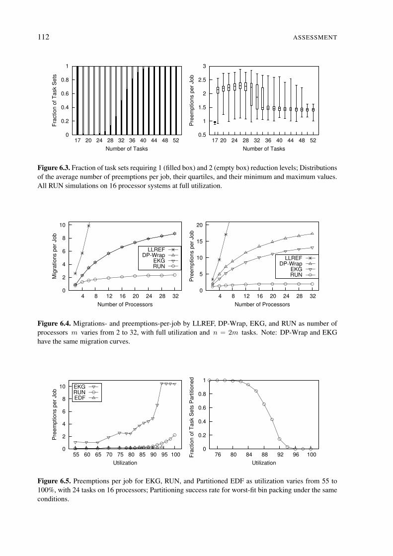
112 ASSESSMENT
0
0.2
0.4
0.6
0.8
1
17 20 24 28 32 36 40 44 48 52
Fra
ctio
n o
f T
ask S
ets
Number of Tasks
0.5
1
1.5
2
2.5
3
17 20 24 28 32 36 40 44 48 52
Pre
em
ptio
ns p
er
Jo
b
Number of Tasks
Figure 6.3. Fraction of task sets requiring 1 (filled box) and 2 (empty box) reduction levels; Distributionsof the average number of preemptions per job, their quartiles, and their minimum and maximum values.All RUN simulations on 16 processor systems at full utilization.
0
2
4
6
8
10
4 8 12 16 20 24 28 32
Mig
ratio
ns p
er
Jo
b
Number of Processors
LLREF DP-Wrap
EKGRUN
0
5
10
15
20
4 8 12 16 20 24 28 32
Pre
em
ptio
ns p
er
Jo
b
Number of Processors
LLREF DP-Wrap
EKGRUN
Figure 6.4. Migrations- and preemptions-per-job by LLREF, DP-Wrap, EKG, and RUN as number ofprocessors m varies from 2 to 32, with full utilization and n “ 2m tasks. Note: DP-Wrap and EKGhave the same migration curves.
0
2
4
6
8
10
55 60 65 70 75 80 85 90 95 100
Pre
em
ptio
ns p
er
Jo
b
Utilization
EKGRUN EDF
0
0.2
0.4
0.6
0.8
1
76 80 84 88 92 96 100Fra
ctio
n o
f T
ask S
ets
Pa
rtitio
ne
d
Utilization
Figure 6.5. Preemptions per job for EKG, RUN, and Partitioned EDF as utilization varies from 55 to100%, with 24 tasks on 16 processors; Partitioning success rate for worst-fit bin packing under the sameconditions.
Chapter
7Reduction to Uniprocessor: a seminal path to optimality.
CONCLUSION
We have presented the optimal RUN multiprocessor real-time scheduling algorithm. RUN trans-
forms the problem of scheduling a set of periodic real-time task with implicit deadlines on two
or more processors into a collection of one or more of the same problem on uniprocessor sys-
tems. As a consequence, the RUN algorithm furnishes a polynomial transformation from the
multiprocessor to the uniprocessor scheduling problem, showing that the first problem is not
more complicated than the latter.
RUN employs a semi-partitioned approach, but partitions tasks among servers rather than
processors. RUN also does not proportional fairness but instead partitioned proportionate fair-
ness. That is, each server generates a job between consecutive deadlines of any client tasks, and
that job is assigned a workload proportional to the server’s rate. Thus, servers globally shares
the total processing bandwidth. As regards the jobs of a server clients, they collectively perform
a proportionally “fair” amount of work between any two client deadlines, but such deadlines do
not demand fairness among the individual client tasks. As a consequence, tasks in different
branches of the server tree may have little influence on each others’ scheduling. This is in stark
contrast to previous optimal algorithms, where every unique system deadline imposes a new
time slice and such slices cause preemptions for many or all tasks.
The limited isolation of groups of tasks provided by server partitioning and the reduced con-
text switching imposed by minimal proportional fairness make RUN significantly more efficient
than previous optimal algorithms.
Instead of statically allocating tasks to specific processors, the approach described in this
work controls migration at run-time via the dual and packing operations. A series of opera-
tion is carried out aiming at transforming a multiprocessor scheduling problem into equivalent
uniprocessor scheduling problems. Like partition-based approaches, solutions to uniproces-
sor scheduling can be used. Differently from other migration-control schemes, the proposed
113
114 CONCLUSION
approach makes use of servers as a means of scheduling transformed systems and generating
migration necessary points.
It is worth emphasizing that the approach being proposed here shares some aspects with
global-based approaches. Among these aspects are the possibility of optimality and the absence
of static allocation to processors.
As regards the overhead of RUN, a theoretical upper bound of Oplogmq average preemp-
tions per job on m processors. Also, extensive simulations have shown that only a few pre-
emption points per job are generated on average, allowing the RUN algorithm to significantly
outperform prior optimal algorithms. Simulations of a varying number of processors have also
shown that RUN scales well as the number of tasks and processors increase.
For non fully-utilized systems, it was shown that the system slack can be efficiently shared
between processors in order to increase the chance for the bin packing procedure to find a proper
partition. In such a case, RUN reduces to the more efficient partitioned approach of Partitioned
EDF.
These results have both practical and theoretical implications. The overhead of RUN is low
enough to justify implementation on actual multiprocessor architectures.
At present, our approach only works for fixed-rate task sets with implicit deadlines. Theo-
retical challenges include extending the model to more general problem domains such as spo-
radic tasks with constrained deadlines.
Also, the use of uniprocessor scheduling results to solve the multiprocessor problem raises
interesting questions in the analysis of fault tolerance, energy consumption and adaptability.
We believe that this novel approach to optimal scheduling introduces a fertile field of re-
search to explore and further build upon. Examples of open research topics could be:
• Avoid the necessity of the reduction tree, or at least, of the dual scheduling level;
• Study the possibility of eliminating some preemption points by skipping unnecessary
deadlines inherited by a server from its clients;
• Explore the impact of using other uniprocessor scheduling algorithm different from EDF
as policy for servers;
• Take profit of the possible slack in the task system to improve bin-packing and/or reduce
the needed number of reduction levels;
• Extend the RUN algorithm to the sporadic task model with implicit or constrained dead-
lines;
• Explore the impact of using some other optimal uniprocessor scheduling algorithm than
EDF as policy for servers;
CONCLUSION 115
• Characterize the impact of the floating point arithmetic or discrete arithmetic used by the
practical multiprocessor system on the schedulability of tasksets using less or 100% of
the processing power.

116 CONCLUSION
BIBLIOGRAPHY
ANDERSON, J.; SRINIVASAN., A. Pfair scheduling: Beyond periodic task systems. In: Pro-
ceedings of the 7th International Conference on Real-time Computing Systems and Applica-
tions. [S.l.: s.n.], 2000. p. 297–306.
ANDERSON, J.; SRINIVASAN., A. Mixed pfair/erfair scheduling of asynchronous periodic
tasks. Journal of Computer and System Sciences, v. 68, p. 157–204, February 2004.
ANDERSSON, B.; BLETSAS, K.; BARUAH, S. Scheduling arbitrary-deadline sporadic task
systems on multiprocessors. In: IEEE RTSS. [S.l.: s.n.], 2008. p. 385–394.
ANDERSSON, B.; TOVAR, E. Multiprocessor scheduling with few preemptions. In: IEEE
Embedded and Real-Time Computing Systems and Applications. [S.l.: s.n.], 2006. p. 322–334.
BARUAH, S. Scheduling periodic tasks on uniform multiprocessors. Inf. Process. Lett., Elsevier
North-Holland, Inc., Amsterdam, The Netherlands, The Netherlands, v. 80, p. 97–104, October
2001. ISSN 0020-0190. Disponível em: ăhttp://dl.acm.org/citation.cfm?id=511722.511727ą.
BARUAH, S.; CHEN, D.; GORINSKY, S.; MOK, A. Generalized multiframe tasks.
Real-Time Systems, Springer Netherlands, v. 17, p. 5–22, 1999. ISSN 0922-6443.
10.1023/A:1008030427220. Disponível em: ăhttp://dx.doi.org/10.1023/A:1008030427220ą.
BARUAH, S.; COHEN, N. K.; PLAXTON, C. G.; VARVEL, D. A. Proportionate progress: a
notion of fairness in resource allocation. Algorithmica, v. 15, n. 6, p. 600–625, 1996.
BARUAH, S.; GEHRKE, J.; PLAXTON, C. Fast scheduling of periodic tasks on multiple re-
sources. In: Proceedings of the 9th International Parallel Processing Symposium. [S.l.: s.n.],
1995. p. 280–288.
BARUAH, S.; GOOSSENS, J. Scheduling real-time tasks: Algorithms and complexity. In: LE-
UNG, J. Y.-T. (Ed.). Handbook of Scheduling: Algorithms, Models, and Performance Analysis.
[S.l.]: Chapman Hall/CRC Press, 2004.
BARUAH, S.; MOK, A.; ROSIER, L. Preemptively scheduling hard-real-time sporadic tasks
on one processor. In: IEEE RTSS. [S.l.: s.n.], 1990. p. 182 –190.
117
118 BIBLIOGRAPHY
BARUAH, S. K.; COHEN, N. K.; PLAXTON, C. G.; VARVEL, D. A. Proportionate progress:
a notion of fairness in resource allocation. In: Proceedings of the twenty-fifth annual ACM
symposium on Theory of computing. New York, NY, USA: ACM, 1993. (STOC ’93), p. 345–
354. ISBN 0-89791-591-7. Disponível em: ăhttp://doi.acm.org/10.1145/167088.167194ą.
BASTONI, A.; BRANDENBURG, B.; ANDERSON, J. Is semi-partitioned scheduling practi-
cal? In: Real-Time Systems (ECRTS), 2011 23rd Euromicro Conference on. [S.l.: s.n.], 2011. p.
125 –135. ISSN 1068-3070.
BERTOGNA, M. Real-Time Scheduling Analysis for Multiprocessor Platforms. Tese
(Doutorado) — Scuola Superiore Sant’Anna, Pisa, 2007.
BOURBAKI, N. Theory of Sets. [S.l.]: Addison-Wesley, 1968. (Elements of Mathematics).
BURNS, A.; WELLINGS, A. Real-Time Systems and Programming Languages. 4. ed. [S.l.]:
Addison Wesley Longmain, 2009.
BUTTAZZO, G. C. Rate monotonic vs. EDF: judgment day. Real-Time Syst., Kluwer Academic
Publishers, Norwell, MA, USA, v. 29, p. 5–26, January 2005. ISSN 0922-6443. Disponível em:
ăhttp://dl.acm.org/citation.cfm?id=1035387.1035388ą.
CARPENTER, J.; FUNK, S.; HOLMAN, P.; SRINIVASAN, A.; ANDERSON, J.; BARUAH,
S. A categorization of real-time multiprocessor scheduling problems and algorithms. In: Hand-
book on Scheduling Algorithms, Methods, and Models. [S.l.]: Chapman Hall/CRC, Boca, 2004.
CHO, H.; RAVINDRAN, B.; JENSEN, E. D. An optimal real-time scheduling algorithm for
multiprocessors. In: IEEE RTSS. [S.l.: s.n.], 2006. p. 101–110.
CHO, S.; LEE, S.-K.; AHN, S.; LIN, K.-J. Efficient real-time scheduling algorithms for mul-
tiprocessor systems. IEICE Trans. Communications, Gothenburg, Sweden, E85-B, n. 12, p.
2859–2867, 2002.
COFFMAN JR., E. G.; GAREY, M. R.; JOHNSON, D. S. Approximation algorithms for bin
packing: a survey. In: . Boston, MA, USA: PWS Publishing Co., 1997. p. 46–93. ISBN
0-534-94968-1. Disponível em: ăhttp://dl.acm.org/citation.cfm?id=241938.241940ą.
DENG, Z.; LIU, J. W.-S.; SUN, J. Scheme for scheduling hard real-time applications in open
system environment. In: ECRTS. [S.l.: s.n.], 1997. p. 191–199.
DERTOUZOS, M.; MOK, A. Multiprocessor Online Scheduling of Hard-Real-Time Tasks.
IEEE Transactions on Software Engineering, IEEE Computer Society, Los Alamitos, CA, USA,
v. 15, n. 12, p. 1497–1506, 1989. ISSN 0098-5589.
DERTOUZOS, M. L. Control robotics: The procedural control of physical processes. In: IFIP
Congress’74. [S.l.: s.n.], 1974. p. 807–813.
BIBLIOGRAPHY 119
EASWARAN, A.; SHIN, I.; LEE, I. Optimal virtual cluster-based multiprocessor scheduling.
Real-Time Syst., Kluwer Academic Publishers, Norwell, MA, USA, v. 43, n. 1, p. 25–59, 2009.
ISSN 0922-6443.
EMBERSON, P.; STAFFORD, R.; DAVIS, R. I. Techniques for the synthesis of multiprocessor
tasksets. In: WATERS. [S.l.: s.n.], 2010. p. 6–11.
EMBERSON, P.; STAFFORD, R.; DAVIS, R. I. A taskset generator for experiments with real-
time task sets. Jan. 2011. http://retis.sssup.it/waters2010/data/taskgen-0.1.tar.gz.
FISHER, N.; GOOSSENS, J.; BARUAH, S. Optimal online multiprocessor scheduling of spo-
radic real-time tasks is impossible. Real-Time Syst., Kluwer Academic Publishers, Norwell,
MA, USA, v. 45, n. 1-2, p. 26–71, 2010. ISSN 0922-6443.
FISHER, N. W. The Multiprocessor Real-Time Scheduling of General Task Systems. Tese
(Doutorado) — University of North Carolina, Chapel Hill, 2007.
FUNAOKA, K.; KATO, S.; YAMASAKI, N. Work-conserving optimal real-time scheduling on
multiprocessors. In: IEEE ECRTS. [S.l.: s.n.], 2008. p. 13–22.
FUNK, S. LRE-TL: An optimal multiprocessor algorithm for sporadic task sets with uncon-
strained deadlines. Real-Time Syst., v. 46, p. 332–359, 2010.
FUNK, S. H. EDF Scheduling on Heterogeneous Multiprocessors. Tese (Doutorado) — Uni-
versity of North Carolina, 2004.
GAREY, M. R.; JOHNSON, D. S. Computers and Intractability: A Guide to the Theory of
NP-Completeness. [S.l.]: W. H. Freeman and Company, 1979.
GEORGE, L.; RIVIERRE, N.; SPURI, M. Preemptive and Non-Preemptive Real-Time Unipro-
cessor Scheduling. [S.l.], 1996.
HILDEBRANDT, J.; GOLATOWSKI, F.; TIMMERMANN, D. Scheduling coprocessor for
enhanced least-laxity-first scheduling in hard real-time systems. Real-Time Systems, Euromicro
Conference on, IEEE Computer Society, Los Alamitos, CA, USA, v. 0, p. 0208, 1999.
HOCHBAUM, D. S. (Ed.). Approximation algorithms for NP-hard problems. Boston, MA,
USA: PWS Publishing Co., 1997. ISBN 0-534-94968-1.
HOLMAN, P.; ANDERSON, J. H. Adapting Pfair Scheduling for Symmetric Multiprocessors.
Journal of Embedded Computing, IOS Press, v. 1, n. 4, p. 543–564, 2005.
HOLMAN, P. L. On the Implementation of Pfair-scheduled Multiprocessor Systems. Tese
(Doutorado) — University of North Carolina, Chapel Hill, 2004.
120 BIBLIOGRAPHY
HONG, K.; LEUNG, J.-T. On-Line Scheduling of Real-Time Tasks. In: In Proceedings of the
Real-Time Systems Symposium. Huntsville, AL, USA: IEEE Computer Society, 1988. p. 244–
250.
HORN, W. A. Some simple scheduling algorithms. Naval Research Logistics Quarterly, Wiley
Subscription Services, Inc., A Wiley Company, v. 21, n. 1, p. 177–185, 1974.
KATO, S.; YAMASAKI, N.; ISHIKAWA, Y. Semi-partitioned scheduling of sporadic task sys-
tems on multiprocessors. In: IEEE ECRTS. [S.l.: s.n.], 2009. p. 249–258.
KOREN, G.; AMIR, A.; DAR, E. The power of migration in multi-processor scheduling of
real-time systems. In: ACM-SIAM symposium on Discrete algorithms. [S.l.: s.n.], 1998. (SODA
’98), p. 226–235.
LEVIN, G.; FUNK, S.; SADOWSKI, C.; PYE, I.; BRANDT, S. DP-FAIR: a simple model for
understanding optimal multiprocessor scheduling. In: IEEE ECRTS. [S.l.: s.n.], 2010. p. 3–13.
LEVIN, G.; SADOWSKI, C.; PYE, I.; BRANDT, S. SNS: a simple model for understanding
optimal hard real-time multi-processor scheduling. [S.l.], 2009.
LIU, C. L. Scheduling algorithms for multiprogram in a hard real-time environment. JPL Space
Programs Summary, II, p. 37–60, 1969.
LIU, C. L.; LAYLAND, J. W. Scheduling algorithms for multiprogram in a hard real-time
environment. Journal of ACM, v. 20, n. 1, p. 40–61, 1973.
LIU, J. W. S. Real-Time Systems. [S.l.]: Prentice-Hall, 2000.
MASSA, E.; LIMA, G. A bandwidth reservation strategy for multiprocessor real-time schedul-
ing. In: IEEE RTAS. [S.l.: s.n.], 2010. p. 175 –183.
MCNAUGHTON, R. Scheduling with deadlines and loss functions. Management Science, v. 6,
n. 1, p. 1–12, 1959.
MOIR, M.; RAMAMURTHY, S. Pfair scheduling of fixed and migrating periodic tasks on
multiple resources. In: IEEE RTSS. [S.l.: s.n.], 1999. p. 294 –303.
MOK, A. K.-L. Fundamental Design Problems of Distributed Systems for the Hard Real-Time
Environment. Tese (Doutorado) — Massachusetts Institute of Technology, 1983.
NELISSEN, G.; BERTEN, V.; GOOSSENS, J.; MILOJEVIC, D. Reducing preemptions and
migrations in real-time multiprocessor scheduling algorithms by releasing the fairness. In: Em-
bedded and Real-Time Computing Systems and Applications (RTCSA), 2011 IEEE 17th Inter-
national Conference on. [S.l.: s.n.], 2011. v. 1, p. 15 –24. ISSN 1533-2306.
BIBLIOGRAPHY 121
PARK, M.; HAN, S.; KIM, H.; CHO, S.; CHO, Y. Zl scheme: Generalization of edzl scheduling
algorithm for real-time multiprocessor systems. Information: An International Interdisciplinary
Journal, v. 8, n. 5, p. 683–691, October 2005.
PIAO, X.; HAN, S.; KIM, H.; PARK, M.; CHO, Y.; CHO, S. Predictability of earliest dead-
line zero laxity algorithm for multiprocessor real-time systems. In: Proc. of the 9th IEEE In-
ternational Symposium on Object and Component-Oriented Real-Time Distributed Computing
(ISORC). [S.l.: s.n.], 2006. p. 359–364.
REGNIER, P.; LIMA, G.; MASSA, E.; LEVIN, G.; BRANDT, S. Run: Optimal multiprocessor
real-time scheduling via reduction to uniprocessor. In: Real-Time Systems Symposium (RTSS),
2011 IEEE 32nd. [S.l.: s.n.], 2011. p. 104 –115. ISSN 1052-8725.
SAHNI, S. Preemptive Scheduling with Due Dates. Operations Research, v. 27, n. 5, p. 925–
934, 1979. Disponível em: ăhttp://or.journal.informs.org/cgi/content/abstract/27/5/925ą.
SPURI, M.; BUTTAZZO, G. Scheduling aperiodic tasks in dynamic priority systems. Real-
Time Syst., v. 10, n. 2, p. 179–210, 1996.
UTHAISOMBUT, P. Generalization of EDF and LLF: Identifying all optimal online algo-
rithms for minimizing maximum lateness. Algorithmica, Springer New York, v. 50, p. 312–328,
2008. ISSN 0178-4617. 10.1007/s00453-007-9083-9. Disponível em: ăhttp://dx.doi.org/10-
.1007/s00453-007-9083-9ą.
ZHU, D.; MOSSÉ, D.; MELHEM, R. Multiple-resource periodic scheduling problem: how
much fairness is necessary? In: IEEE RTSS. Washington, DC, USA: IEEE Computer Soci-
ety, 2003. p. 142–151. ISBN 0-7695-2044-8. Disponível em: ăhttp://portal.acm.org/citation-
.cfm?id=956418.956616ą.
ZHU, D.; QI, X.; MOSSÉ, D.; MELHEM, R. An optimal boundary fair scheduling algorithm
for multiprocessor real-time systems. Journal of Parallel and Distributed Computing, v. 71,
n. 10, p. 1411 – 1425, 2011. ISSN 0743-7315.

122 BIBLIOGRAPHY

APPENDIX

124 BIBLIOGRAPHY
Appendix
AScheduling idle time is somehow equivalent to scheduling execution time.
IDLE SERIALIZATION
During the first two years of this PhD research, we have been actively working on the idea of
scheduling both execution and idle times in order to improve the efficiency for generating a
schedule.
As a first attempt of idle scheduling procedure, we have developed a new approach based
on serializing idle time. We give here a brief description of this idle serialization approach,
since this idea has finally led us to devise our actual proposal, RUN, an optimal algorithm for
periodic task set with implicit deadlines.
We warn the reader that the material presented here has not be validated by any referee
based procedure. Thus, it may contain some imprecision. However, since we have developed
an algorithm based on idle serialization and estimated its efficiency through simulations, we
find it convenient to expose this material here.
A.1 FRAME
Time is mapped to the non-negative real set and time intervals are the usual intervals of R.
We call frame, denoted rs, fqk, the execution time available on a processor Pk during time
interval rs, fq . An idle frame is one during which no job executes. We denote rs, fqk,i the
frame in processor during which job Ji executes continuously.
At any time t, a scheduling policy assigns frames to the current active jobs. The set of
active jobs at t, denoted Aptq, represents all jobs released at or before t but not yet finished by
t. Note that Aptq contains jobs partially executed by t and so, can be defined as the set of jobs
such that Ji.r ď t and epJi, tq ą 0.
125
126 IDLE SERIALIZATION
Definition A.1.1 (Serialized, Parallel, Concurrent and Adjacent Frames). Consider two frames
Fj “ rs, fqj and Fk “ rs1, f 1qk on two processors Pj and Pk, respectively.
•Fj and Fk are serialized if both j “ k and rs, fq X rs1, f 1q “ tu;
•Fj and Fk are serializable if rs, fq X rs1, f 1q “ tu. In words, serializable frames are
those that can be serialized in the same processor;
•Fj and Fk are adjacent if Fj and Fk are serialized and if f “ s1 or f 1 “ s.
A.2 MAPPING
Definition A.2.1 (Mapping of a job). A mapping of a job Ji on a multiprocessor system Π,
denoted Miptq, is a set of frames reserved at time t on a subset of Π for the future execution
of Ji such that:
•The first frame of Miptq begins after the release time of Ji;
•The frames of Miptq are pairwise serializable and they do not overlap with frames of any
other mapping;
•The cumulative length of all frames of Miptq equals epJi, tq.
Upon arrival of a job Ji at time t, three scenarios are possible. First, a mapping may be
assigned to Ji immediately. Second, Ji may be rejected according to some admission criterion.
Third, the mapping assignment of Ji may be delayed to some future instant. In this later case,
Ji remains in the ready queue Qptq until the eventual assignment of a mapping to Ji or the
rejection of Ji. Thus, Qptq is the set of released jobs at t, not yet mapped nor rejected.
Definition A.2.2 (Map). A map Mptq at time t is the set of all mappings defined on Π at t.
Formally,
Mptq “ tMiptq, Ji P J zQptq ^ ri ď tu
A processor map Mkptq is the set of all frames of Mptq reserved on processor Pk for the
execution of some job. Formally,
Mkptq “ tF P Mptq, F X r0,`8qk “ F u
For example, consider the 3-task set T “ tτ1 :p2, 3q, τ2 :p2, 3q, τ3 :p4, 6qu . The mappings
assigned to J1 :p0, 2, 3q and J2 :p0, 2, 3q by EDF are shown in Figure A.1a. The resulting
processor maps M1p0q and M2p0q equals tr0, 2q1,1u and tr0, 2q2,2u, respectively; the map
Mp0q equals M1p0q Y M2p0q and the ready queue Qp0q equals tJ3 :p0, 4, 6qu.
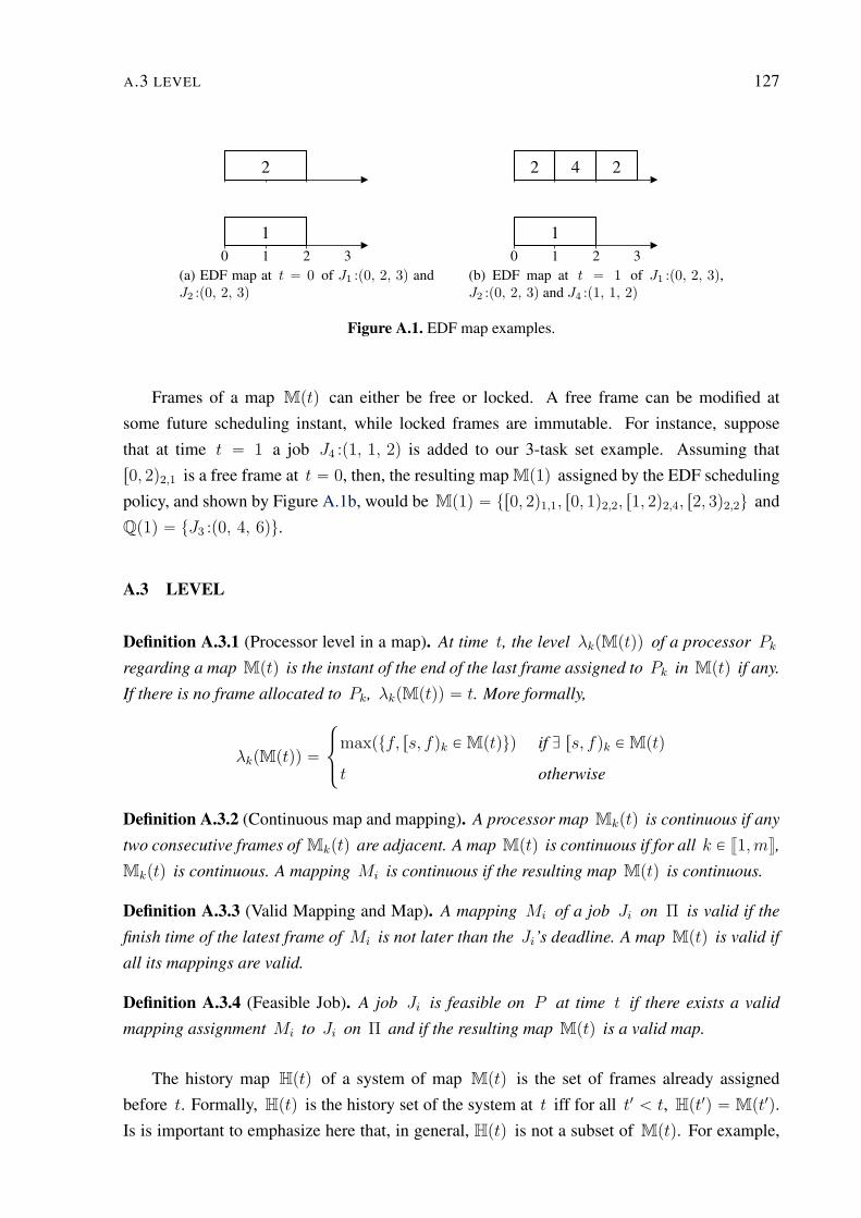
A.3 LEVEL 127
0 1 2 3
1
2
(a) EDF map at t “ 0 of J1 :p0, 2, 3q andJ2 :p0, 2, 3q
0 1 2 3
1
2 4 2
(b) EDF map at t “ 1 of J1 :p0, 2, 3q,J2 :p0, 2, 3q and J4 :p1, 1, 2q
Figure A.1. EDF map examples.
Frames of a map Mptq can either be free or locked. A free frame can be modified at
some future scheduling instant, while locked frames are immutable. For instance, suppose
that at time t “ 1 a job J4 :p1, 1, 2q is added to our 3-task set example. Assuming that
r0, 2q2,1 is a free frame at t “ 0, then, the resulting map Mp1q assigned by the EDF scheduling
policy, and shown by Figure A.1b, would be Mp1q “ tr0, 2q1,1, r0, 1q2,2, r1, 2q2,4, r2, 3q2,2u and
Qp1q “ tJ3 :p0, 4, 6qu.
A.3 LEVEL
Definition A.3.1 (Processor level in a map). At time t, the level λkpMptqq of a processor Pk
regarding a map Mptq is the instant of the end of the last frame assigned to Pk in Mptq if any.
If there is no frame allocated to Pk, λkpMptqq “ t. More formally,
λkpMptqq “
$
&
%
maxptf, rs, fqk P Mptquq if D rs, fqk P Mptq
t otherwise
Definition A.3.2 (Continuous map and mapping). A processor map Mkptq is continuous if any
two consecutive frames of Mkptq are adjacent. A map Mptq is continuous if for all k P v1,mw,
Mkptq is continuous. A mapping Mi is continuous if the resulting map Mptq is continuous.
Definition A.3.3 (Valid Mapping and Map). A mapping Mi of a job Ji on Π is valid if the
finish time of the latest frame of Mi is not later than the Ji’s deadline. A map Mptq is valid if
all its mappings are valid.
Definition A.3.4 (Feasible Job). A job Ji is feasible on P at time t if there exists a valid
mapping assignment Mi to Ji on Π and if the resulting map Mptq is a valid map.
The history map Hptq of a system of map Mptq is the set of frames already assigned
before t. Formally, Hptq is the history set of the system at t iff for all t1 ă t, Hpt1q “ Mpt1q.
Is is important to emphasize here that, in general, Hptq is not a subset of Mptq. For example,
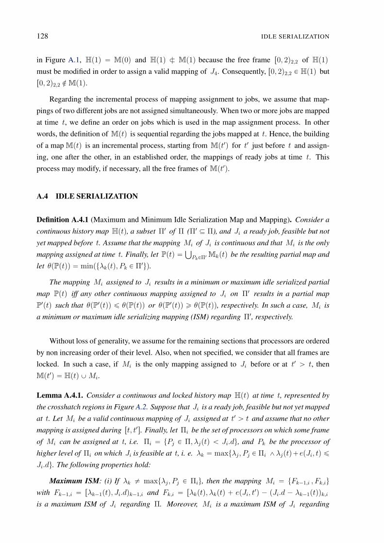
128 IDLE SERIALIZATION
in Figure A.1, Hp1q “ Mp0q and Hp1q Ć Mp1q because the free frame r0, 2q2,2 of Hp1q
must be modified in order to assign a valid mapping of J4. Consequently, r0, 2q2,2 P Hp1q but
r0, 2q2,2 R Mp1q.
Regarding the incremental process of mapping assignment to jobs, we assume that map-
pings of two different jobs are not assigned simultaneously. When two or more jobs are mapped
at time t, we define an order on jobs which is used in the map assignment process. In other
words, the definition of Mptq is sequential regarding the jobs mapped at t. Hence, the building
of a map Mptq is an incremental process, starting from Mpt1q for t1 just before t and assign-
ing, one after the other, in an established order, the mappings of ready jobs at time t. This
process may modify, if necessary, all the free frames of Mpt1q.
A.4 IDLE SERIALIZATION
Definition A.4.1 (Maximum and Minimum Idle Serialization Map and Mapping). Consider a
continuous history map Hptq, a subset Π1 of Π (Π1 Ď Π), and Ji a ready job, feasible but not
yet mapped before t. Assume that the mapping Mi of Ji is continuous and that Mi is the only
mapping assigned at time t. Finally, let Pptq “Ť
PkPΠ1 Mkptq be the resulting partial map and
let θpPptqq “ minptλkptq, Pk P Π1uq.
The mapping Mi assigned to Ji results in a minimum or maximum idle serialized partial
map Pptq iff any other continuous mapping assigned to Ji on Π1 results in a partial map
P1ptq such that θpP1ptqq ď θpPptqq or θpP1ptqq ě θpPptqq, respectively. In such a case, Mi is
a minimum or maximum idle serializing mapping (ISM) regarding Π1, respectively.
Without loss of generality, we assume for the remaining sections that processors are ordered
by non increasing order of their level. Also, when not specified, we consider that all frames are
locked. In such a case, if Mi is the only mapping assigned to Ji before or at t1 ą t, then
Mpt1q “ Hptq Y Mi.
Lemma A.4.1. Consider a continuous and locked history map Hptq at time t, represented by
the crosshatch regions in Figure A.2. Suppose that Ji is a ready job, feasible but not yet mapped
at t. Let Mi be a valid continuous mapping of Ji assigned at t1 ą t and assume that no other
mapping is assigned during rt, t1s. Finally, let Πi be the set of processors on which some frame
of Mi can be assigned at t, i.e. Πi “ tPj P Π, λjptq ă Ji.du, and Pk be the processor of
higher level of Πi on which Ji is feasible at t, i. e. λk “ maxtλj, Pj P Πi ^λjptq`epJi, tq ď
Ji.du. The following properties hold:
Maximum ISM: (i) If λk ‰ maxtλj, Pj P Πiu, then the mapping Mi “ tFk´1,i , Fk,iu
with Fk´1,i “ rλk´1ptq, Ji.dqk´1,i and Fk,i “ rλkptq, λkptq ` epJi, t1q ´ pJi.d ´ λk´1ptqqk,i
is a maximum ISM of Ji regarding Π. Moreover, Mi is a maximum ISM of Ji regarding
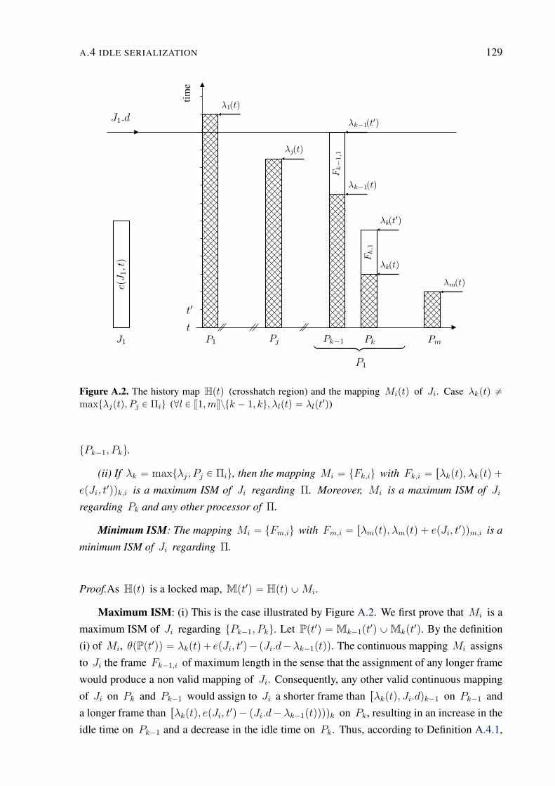
A.4 IDLE SERIALIZATION 129
J1.d
t
t1
tim
e
P1 Pj Pk´1 Pk Pm
epJ
1,t
q
J1
λ1ptq
λjptq
λk´1ptq
λkptq
λmptq
Fk
´1,1
λk´1pt1q
Fk,1
λkpt1q
looooooooooomooooooooooon
P1
Figure A.2. The history map Hptq (crosshatch region) and the mapping Miptq of Ji. Case λkptq ‰maxtλjptq, Pj P Πiu (@l P v1,mwztk ´ 1, ku, λlptq “ λlpt
1q)
tPk´1, Pku.
(ii) If λk “ maxtλj, Pj P Πiu, then the mapping Mi “ tFk,iu with Fk,i “ rλkptq, λkptq `
epJi, t1qqk,i is a maximum ISM of Ji regarding Π. Moreover, Mi is a maximum ISM of Ji
regarding Pk and any other processor of Π.
Minimum ISM: The mapping Mi “ tFm,iu with Fm,i “ rλmptq, λmptq ` epJi, t1qqm,i is a
minimum ISM of Ji regarding Π.
Proof.As Hptq is a locked map, Mpt1q “ Hptq Y Mi.
Maximum ISM: (i) This is the case illustrated by Figure A.2. We first prove that Mi is a
maximum ISM of Ji regarding tPk´1, Pku. Let Ppt1q “ Mk´1pt1q Y Mkpt1q. By the definition
(i) of Mi, θpPpt1qq “ λkptq ` epJi, t1q ´ pJi.d´λk´1ptqq. The continuous mapping Mi assigns
to Ji the frame Fk´1,i of maximum length in the sense that the assignment of any longer frame
would produce a non valid mapping of Ji. Consequently, any other valid continuous mapping
of Ji on Pk and Pk´1 would assign to Ji a shorter frame than rλkptq, Ji.dqk´1 on Pk´1 and
a longer frame than rλkptq, epJi, t1q ´ pJi.d´ λk´1ptqqqqk on Pk, resulting in an increase in the
idle time on Pk´1 and a decrease in the idle time on Pk. Thus, according to Definition A.4.1,
130 IDLE SERIALIZATION
Mi is the maximum ISM of Ji regarding tPk´1, Pku.
To prove that Mi is the maximum ISM of Ji regarding Π, we distinguish two cases. First,
if k ‰ m, then θpMpt1qq “ λmptq and Mi is a maximum ISM regarding Π. Second, if k “ m,
then λmpt1q “ λmptq ` epJi, t1q ´ pJi.d ´ λm´1ptqq and we have mintλjpt
1q, j P v1,mwu “
λmpt1q because λmpt1q ă λm´1ptq, by the definition of Mi. Hence, θpMpt1qq “ λmpt1q which
proves that, in this case also, Mi is a maximum ISM regarding Π.
(ii) Let Pj be a processor different from Pk. We must prove that Mi is a maximum ISM
regarding tPj, Pku. However, as Ji is feasible on Pk, the mapping Mi defined by (ii) is valid.
Moreover, as Mi defined by (ii) is the only continuous mapping of Ji on the single processor
Pk, the assignment of part of the execution time of Ji to another frame Fj,i on Pj ‰ Pk would
result in an later idle time on Pj . Thus, according to A.4.1, Mi is the maximum ISM of Jiregarding tPj, Pku.
Minimum ISM: Here again, we distinguish two cases. First, if λmptq ` epJi, t1qqm,i ď
λm´1ptq, then θpMpt1q “ λmpt1q. Thus, any other mapping of Ji would result in an earlier
idle time on Pm. Otherwise, θpMpt1qq “ λm´1ptq. However, as Mi is continuous, the only
frame that could be assigned to Pm´1 by another mapping of Ji would be rλm´1ptq, λm´1ptq`
epJi, t1q ´ pλm´1ptq ´ λmptqqqm´1,i. But, such an assignment would result in the same value of
θpMpt1qq that would be achieve on Pm instead of Pm´1. This establishes the Lemma.
Given an history map at time t, Lemma A.4.1 characterizes which different mappings of a
job achieved minimum and maximum idle serialization. The next lemma quantifies the differ-
ences between each of this mappings in terms of idle serialization.
Lemma A.4.2. Consider the minimum and maximum ISM of a ready job Ji P Qptq on two
processors Pj and Pk at time t. The length δ of the idle time that happens earlier in the maximum
ISM of Ji than in the minimum ISM of Ji is δ “ minpepJi, tq, pλj ´ λkq ´ maxp0, epJi, tq ´
pJi.d ´ λjptqqq.
Proof.This is a consequence of the Definition of maximum and minimum ISM, as illustrated in
Figure A.3. Note that we must distinguish whether λj ` epJi, tq ě Ji.d or not.
A.5 ON-LINE SCHEDULING
We enunciate here the criterion of an on-line scheduling policy for the Idle Serialization
Based (ISBa) scheduling algorithm. When a job Ji P Qptq is considered for mapping at
time t, ISBa needs to choose between the maximum or minimum idle serialization mapping.
However each of this two choices has consequences. Choosing the maximum ISM scenario
may make a ready job feasible, taking advantage of the full length of the longest idle time. On
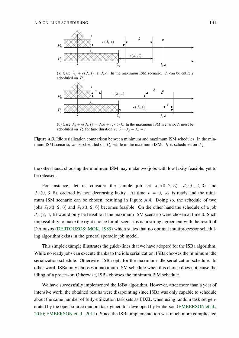
A.5 ON-LINE SCHEDULING 131
Pj
Pk
t λj
λk
epJi, tq
epJi, tq
δ
Ji.d
(a) Case λj ` epJi, tq ď Ji.d. In the maximum ISM scenario, Ji can be entirelyscheduled on Pj .
Pj
Pk
t λj
λk
epJi, tq
epJi, tqr
r δ
Ji.d
(b) Case λj ` epJi, tq “ Ji.d ` r, r ą 0. In the maximum ISM scenario, Ji must bescheduled on Pk for time duration r. δ “ λj ´ λk ´ r
Figure A.3. Idle serialization comparison between minimum and maximum ISM schedules. In the min-imum ISM scenario, Ji is scheduled on Pk while in the maximum ISM, Ji is scheduled on Pj .
the other hand, choosing the minimum ISM may make two jobs with low laxity feasible, yet to
be released.
For instance, let us consider the simple job set J1 :p0, 2, 3q, J2 :p0, 2, 3q and
J3 :p0, 3, 6q, ordered by non decreasing laxity. At time t “ 0, J3 is ready and the mini-
mum ISM scenario can be chosen, resulting in Figure A.4. Doing so, the schedule of two
jobs J4 :p3, 2, 6q and J5 :p3, 2, 6q becomes feasible. On the other hand the schedule of a job
J4 :p2, 4, 6q would only be feasible if the maximum ISM scenario were chosen at time 0. Such
impossibility to make the right choice for all scenarios is in strong agreement with the result of
Dertouzos (DERTOUZOS; MOK, 1989) which states that no optimal multiprocessor schedul-
ing algorithm exists in the general sporadic job model.
This simple example illustrates the guide-lines that we have adopted for the ISBa algorithm.
While no ready jobs can execute thanks to the idle serialization, ISBa chooses the minimum idle
serialization schedule. Otherwise, ISBa opts for the maximum idle serialization schedule. In
other word, ISBa only chooses a maximum ISM schedule when this choice does not cause the
idling of a processor. Otherwise, ISBa chooses the minimum ISM schedule.
We have successfully implemented the ISBa algorithm. However, after more than a year of
intensive work, the obtained results were disapointing since ISBa was only capable to schedule
about the same number of fully-utilization task sets as EDZL when using random task set gen-
erated by the open-source random task generator developed by Emberson (EMBERSON et al.,
2010; EMBERSON et al., 2011). Since the ISBa implementation was much more complicated
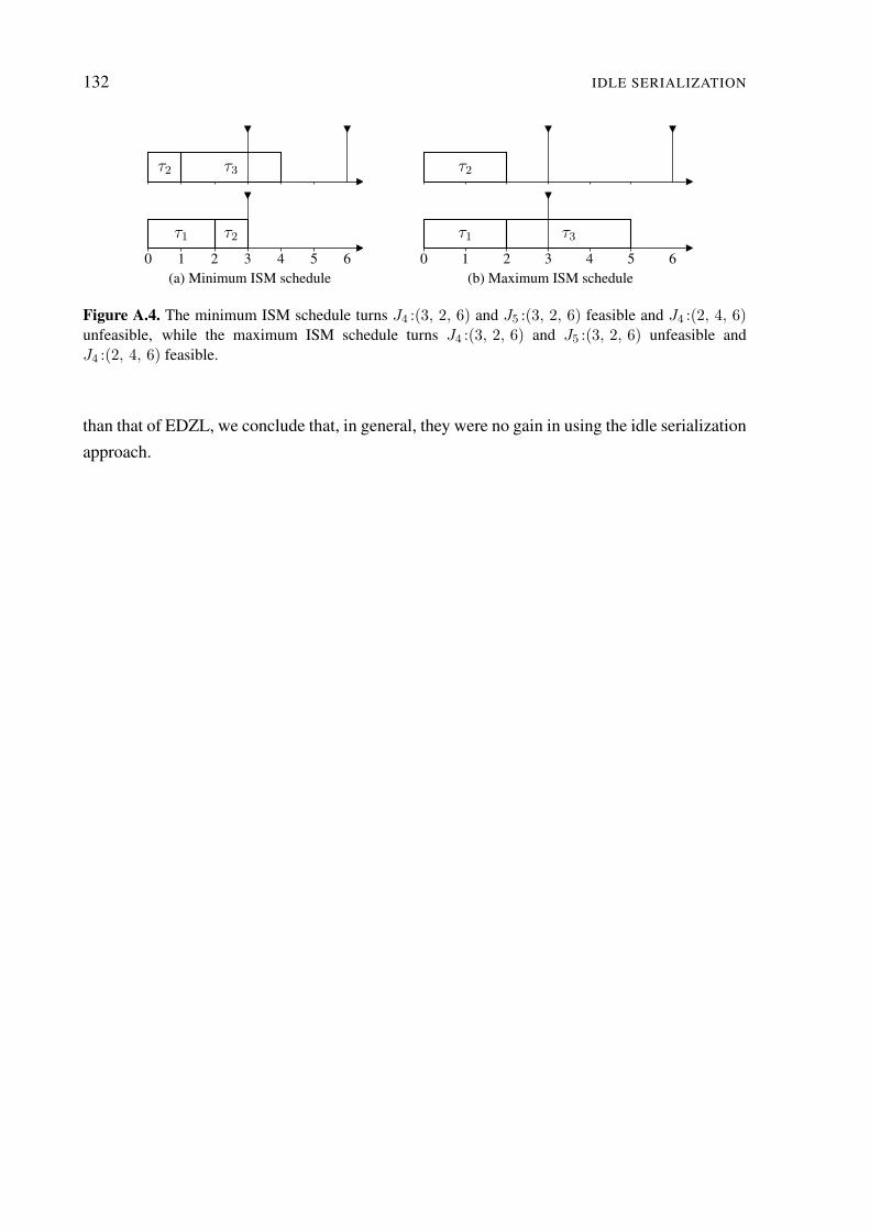
132 IDLE SERIALIZATION
0 1 2 3 4 5 6
τ1 τ2
τ2 τ3
(a) Minimum ISM schedule0 1 2 3 4 5 6
τ1
τ2
τ3
(b) Maximum ISM schedule
Figure A.4. The minimum ISM schedule turns J4 :p3, 2, 6q and J5 :p3, 2, 6q feasible and J4 :p2, 4, 6qunfeasible, while the maximum ISM schedule turns J4 :p3, 2, 6q and J5 :p3, 2, 6q unfeasible andJ4 :p2, 4, 6q feasible.
than that of EDZL, we conclude that, in general, they were no gain in using the idle serialization
approach.
Appendix
BElegance likes shortness. Beauty do not necessarily.
EDF SERVER THEOREM: ANOTHER PROOF
In order to give a direct proof of Theorem 3.4.1, we first present some intermediate results.
B.1 SCALING
Definition B.1.1. Let S be a server, Γ a set of servers with ρpΓq ď 1, and α a real such that
0 ă α ď 1 ρpSq. The α-scaled server of S, denoted αS, is the server with utilization α ρpSq
and deadlines equal to those of S. The α-scaled set of Γ is the set of the α-scaled servers of
all servers in Γ.
As illustration, consider Γ “ tS1, S2, S3u a set of servers with ρpS1q “ 0.1, ρpS2q “ 0.15 ,
ρpS3q “ 0.25 and ρpΓq “ 0.5. The 2-scaled set of Γ is Γ1 “ tS 11, S 1
2, S 1
3u with ρpΓ1q “ 1,
ρpS 11q “ 0.2, ρpS 1
2q “ 0.3 and ρpS 1
3q “ 0.5.
Lemma B.1.1. Let Γ be a set of EDF servers with ρpΓq ď 1. Consider the EDF servers S
and S 1 associated to Γ and Γ1 where Γ1 is α-scaled set of Γ and let Σ and Σ1 are their
corresponding schedules, respectively. Then Σ is valid if and only if Σ1 is valid.
Proof.Suppose that Σ is valid. Consider a deadline d in RpSqzt0u. Since S and S 1 use EDF
and RpSq “ RpS 1q, S and S 1 execute their client jobs in the same order. As a consequence,
all the executions of servers in clipSq during r0, dq must have a corresponding execution of a
server in clipS 1q during r0, dq.
Also, since S executes for ρpSqd during r0, dq and α ď 1 ρpSq, the execution time
ρpS 1qd of S 1 during r0, dq satisfies α ρpSqd ď d. Hence, a client job of S 1 corresponding to
133
134 EDF SERVER THEOREM: ANOTHER PROOF
an execution which completes in Σ before d, completes before d in Σ1. Hence, since Σ is
valid, so is Σ1 .
The converse also follows from the above argument, using a scale factorale equal to α1 “
1α.
B.2 DIRECT PROOF OF THE EDF SERVER THEOREM
The proof presented now of Theorem 3.4.1 is an adaptation of the proof of Theorem 7 from
(LIU; LAYLAND, 1973). Since our server model is a generalization of the PPID task model,
this direct proof does not use more recent results established for this model.
Lemma B.2.1. The unit EDF server S “ serpΓq of a set of synchronous servers Γ with
ρpΓq “ 1 produces a valid schedule of Γ if all jobs of S meet their deadlines.
Proof.We proceed by contradiction.
Assume that there exists an instant D in RpSq at which a deadline miss occurs for a budget
job J of some client server of S in Γ. Also, without loss of generality, assume that no deadline
miss occurs before D i.e., J is the first job after time t “ 0 which misses its deadline at time
D “ J.d.
We define t1 as the start time of the latest idle time interval before J.d if such idle time
exists and t1 “ 0 otherwise. Consider D1 the earliest deadline in RpSq after or at t1. It
must be that D1 ă D otherwise no job of server in Γ would be released between t1 and D,
contradicting the fact that J misses its deadline at time D.
If D1 is not equal to zero, then the processor must be idle during rt1, D1q. Indeed, if there
were some job J 1 executing just before D1, it would have been released after t1 since t1 is the
start time of an idle time. Consequently, the release instant of J 1 would be a deadline in RpSq
occurring before D1 and after t1, which would contradict the definition of D1.
We now show that the total demand of servers in Γ within interval rD1, Dq is not greater
than D ´ D1 , reaching a contradiction, since no idle time exists within rD1, Dq. There are
two cases to be distinguished depending on whether some lower priority server executes within
rD1, Dq.
Case 1
Illustrated by Figure B.1. Assume that no job of servers in Γ with lower priority than J
executes within rD1, Dq. Since there is no processor idle time within rD1, Dq and a deadline
miss occurs at time D, it must be that the accumulated execution time of all budget jobs in Γ
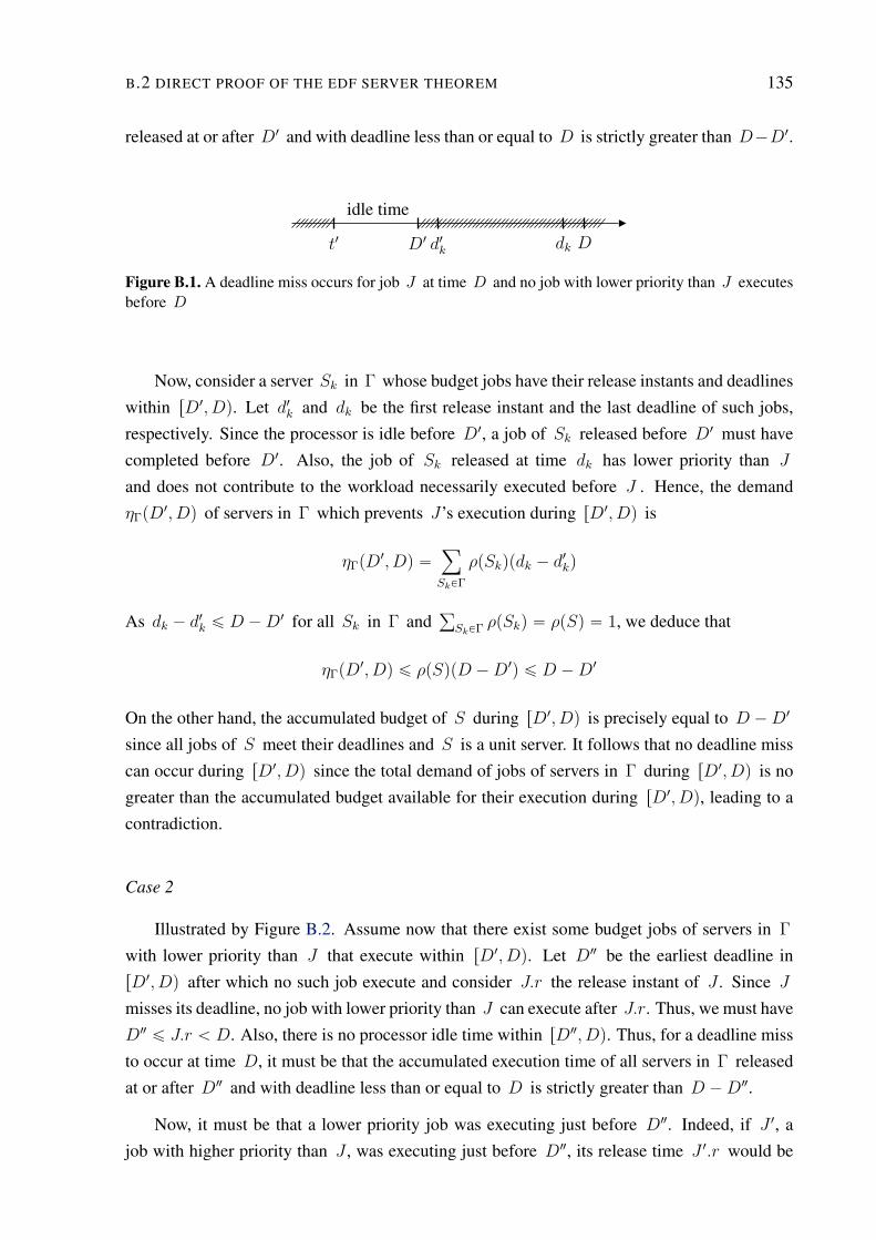
B.2 DIRECT PROOF OF THE EDF SERVER THEOREM 135
released at or after D1 and with deadline less than or equal to D is strictly greater than D´D1.
idle time
t1 D1 d1k dk D
Figure B.1. A deadline miss occurs for job J at time D and no job with lower priority than J executesbefore D
Now, consider a server Sk in Γ whose budget jobs have their release instants and deadlines
within rD1, Dq. Let d1k and dk be the first release instant and the last deadline of such jobs,
respectively. Since the processor is idle before D1, a job of Sk released before D1 must have
completed before D1. Also, the job of Sk released at time dk has lower priority than J
and does not contribute to the workload necessarily executed before J . Hence, the demand
ηΓpD1, Dq of servers in Γ which prevents J’s execution during rD1, Dq is
ηΓpD1, Dq “ÿ
SkPΓ
ρpSkqpdk ´ d1kq
As dk ´ d1k ď D ´ D1 for all Sk in Γ and
ř
SkPΓ ρpSkq “ ρpSq “ 1, we deduce that
ηΓpD1, Dq ď ρpSqpD ´ D1q ď D ´ D1
On the other hand, the accumulated budget of S during rD1, Dq is precisely equal to D ´ D1
since all jobs of S meet their deadlines and S is a unit server. It follows that no deadline miss
can occur during rD1, Dq since the total demand of jobs of servers in Γ during rD1, Dq is no
greater than the accumulated budget available for their execution during rD1, Dq, leading to a
contradiction.
Case 2
Illustrated by Figure B.2. Assume now that there exist some budget jobs of servers in Γ
with lower priority than J that execute within rD1, Dq. Let D2 be the earliest deadline in
rD1, Dq after which no such job execute and consider J.r the release instant of J . Since J
misses its deadline, no job with lower priority than J can execute after J.r. Thus, we must have
D2 ď J.r ă D. Also, there is no processor idle time within rD2, Dq. Thus, for a deadline miss
to occur at time D, it must be that the accumulated execution time of all servers in Γ released
at or after D2 and with deadline less than or equal to D is strictly greater than D ´ D2.
Now, it must be that a lower priority job was executing just before D2. Indeed, if J 1, a
job with higher priority than J , was executing just before D2, its release time J 1.r would be
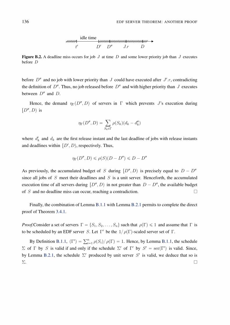
136 EDF SERVER THEOREM: ANOTHER PROOF
idle time
t1 D1 D2 J.r D
Figure B.2. A deadline miss occurs for job J at time D and some lower priority job than J executesbefore D
before D2 and no job with lower priority than J could have executed after J 1.r, contradicting
the definition of D2. Thus, no job released before D2 and with higher priority than J executes
between D2 and D.
Hence, the demand ηΓpD2, Dq of servers in Γ which prevents J’s execution during
rD2, Dq is
ηΓpD2, Dq “ÿ
SkPΓ
ρpSkqpdk ´ d2kq
where d1k and dk are the first release instant and the last deadline of jobs with release instants
and deadlines within rD1, Dq, respectively. Thus,
ηΓpD2, Dq ď ρpSqpD ´ D2q ď D ´ D2
As previously, the accumulated budget of S during rD2, Dq is precisely equal to D ´ D2
since all jobs of S meet their deadlines and S is a unit server. Henceforth, the accumulated
execution time of all servers during rD2, Dq in not greater than D ´ D2, the available budget
of S and no deadline miss can occur, reaching a contradiction.
Finally, the combination of Lemma B.1.1 with Lemma B.2.1 permits to complete the direct
proof of Theorem 3.4.1.
Proof.Consider a set of servers Γ “ tS1, S2, . . . , Snu such that ρpΓq ď 1 and assume that Γ is
to be scheduled by an EDF server S. Let Γ1 be the 1 ρpΓq-scaled server set of Γ.
By Definition B.1.1, pΓ1q “řn
i“1ρpSiq ρpΓq “ 1. Hence, by Lemma B.1.1, the schedule
Σ of Γ by S is valid if and only if the schedule Σ1 of Γ1 by S 1 “ serpΓ1q is valid. Since,
by Lemma B.2.1, the schedule Σ1 produced by unit server S 1 is valid, we deduce that so is
Σ.
Appendix
CWhy shall one use a complex solution whenever a simple exists?
X-RUN: A PROPOSAL FOR SPORADIC TASKS
In this appendix, we discuss some of our ideas to extend RUN to the sporadic task model with
implicit deadlines. Since none of the material presented here is confirmed by theoretical proofs
or simulation results, we can not guarantee its correctness. However, we believe that an optimal
solution for scheduling sporadic task systems with implicit deadlines should emerge soon from
this documented discussion.
C.1 TASK MODEL
We consider a sporadic task model with implicit deadline, further referred as STID model.
According to this model, two jobs of a task τi of period Ti are separated by at least Ti. That
is, Ti is the minimum inter-arrival time between any two jobs of task τi . Formally, if Jk and
Jk`1 are two consecutive jobs of task τi , then Jk`1.r´ Jk.r ě Ti . Note that, since we assume
implicit deadlines, for any job Jk of a task τi, we have Jk.d “ Jk.r ` Ti .
We say that a server Si is active whenever there are one or more client’s jobs of Si ready
to execute. Otherwise, we say that Si is idle.
C.2 RUN SUBTREE
One of the key idea we want to present here for the extension of RUN to the STID model is
based on the concept of subtree that we recall now.
As stated by Definition 5.3.1, a RUN subtree of a general RUN tree is comprised of a single
grandparent server, referred to as root server of the subtree, together with its child servers and
grandchild servers.
137
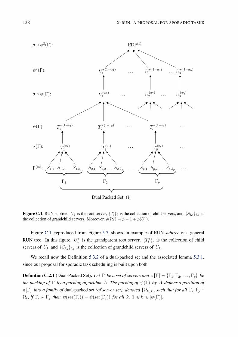
138 X-RUN: A PROPOSAL FOR SPORADIC TASKS
σ ˝ ψ2pΓq:
ψ2pΓq:
σ ˝ ψpΓq:
EDFp1q
U˚ p1´w1q1
. . . U˚ p1´wiqi . . . U
˚ p1´wqqq
Upw1q1
. . . Upwiq2
. . . Upwqqq
ψpΓq: T˚ p1´v1q1
T˚ p1´v2q2
. . . T˚ p1´vpqp
. . .
σpΓq: Tpv1q1
Tpv2q2
. . . Tpvpqp
. . .
Γpmq: S1,1 S1,2 . . . S1,k1 S2,1 S2,2 . . . S2,k2 . . . Sp,1 Sp,2 . . . Sp,kp . . .
Γ1 Γ2 Γp
Dual Packed Set Ω1
Figure C.1. RUN subtree. U1 is the root server, tTiui is the collection of child servers, and tSi,jui,j isthe collection of grandchild servers. Moreover, ρpΩ1q “ p´ 1 ` ρpU1q.
Figure C.1, reproduced from Figure 5.7, shows an example of RUN subtree of a general
RUN tree. In this figure, U˚1
is the grandparent root server, tT ˚i ui is the collection of child
servers of U1, and tSi,jui,j is the collection of grandchild servers of U1.
We recall now the Definition 5.3.2 of a dual-packed set and the associated lemma 5.3.1,
since our proposal for sporadic task scheduling is built upon both.
Definition C.2.1 (Dual-Packed Set). Let Γ be a set of servers and πrΓs “ tΓ1,Γ2, . . . ,Γpu be
the packing of Γ by a packing algorithm A. The packing of ψpΓq by A defines a partition of
πrΓs into a family of dual-packed set (of server set), denoted tΩkuk , such that for all Γi,Γj P
Ωk, if Γi ‰ Γj then ψpserpΓiqq “ ψpserpΓjqq for all k, 1 ď k ď |ψpΓq|.
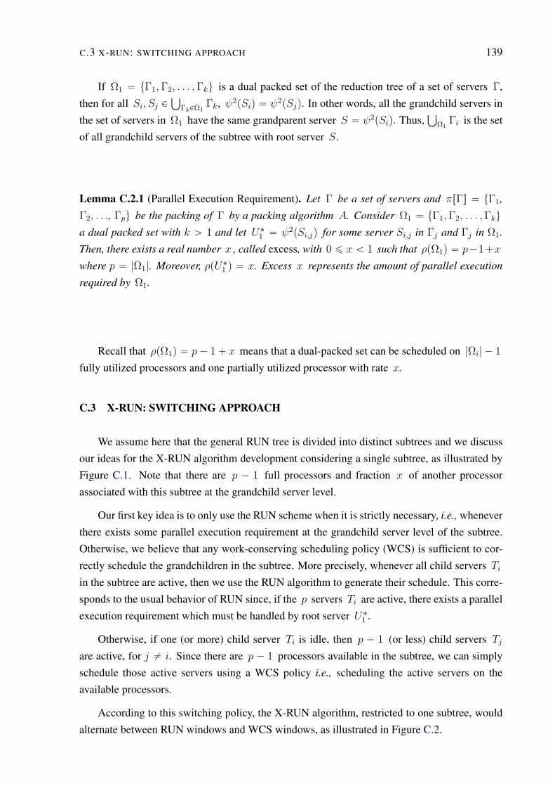
C.3 X-RUN: SWITCHING APPROACH 139
If Ω1 “ tΓ1,Γ2, . . . ,Γku is a dual packed set of the reduction tree of a set of servers Γ,
then for all Si, Sj PŤ
ΓkPΩ1Γk, ψ2pSiq “ ψ2pSjq. In other words, all the grandchild servers in
the set of servers in Ω1 have the same grandparent server S “ ψ2pSiq. Thus,Ť
Ω1Γi is the set
of all grandchild servers of the subtree with root server S.
Lemma C.2.1 (Parallel Execution Requirement). Let Γ be a set of servers and πrΓs “ tΓ1,
Γ2, . . ., Γpu be the packing of Γ by a packing algorithm A. Consider Ω1 “ tΓ1,Γ2, . . . ,Γku
a dual packed set with k ą 1 and let U˚1
“ ψ2pSi,jq for some server Si,j in Γj and Γj in Ω1.
Then, there exists a real number x , called excess, with 0 ď x ă 1 such that ρpΩ1q “ p´1`x
where p “ |Ω1|. Moreover, ρpU˚1
q “ x. Excess x represents the amount of parallel execution
required by Ω1.
Recall that ρpΩ1q “ p´ 1 ` x means that a dual-packed set can be scheduled on |Ωi| ´ 1
fully utilized processors and one partially utilized processor with rate x.
C.3 X-RUN: SWITCHING APPROACH
We assume here that the general RUN tree is divided into distinct subtrees and we discuss
our ideas for the X-RUN algorithm development considering a single subtree, as illustrated by
Figure C.1. Note that there are p ´ 1 full processors and fraction x of another processor
associated with this subtree at the grandchild server level.
Our first key idea is to only use the RUN scheme when it is strictly necessary, i.e., whenever
there exists some parallel execution requirement at the grandchild server level of the subtree.
Otherwise, we believe that any work-conserving scheduling policy (WCS) is sufficient to cor-
rectly schedule the grandchildren in the subtree. More precisely, whenever all child servers Tiin the subtree are active, then we use the RUN algorithm to generate their schedule. This corre-
sponds to the usual behavior of RUN since, if the p servers Ti are active, there exists a parallel
execution requirement which must be handled by root server U˚1
.
Otherwise, if one (or more) child server Ti is idle, then p ´ 1 (or less) child servers Tj
are active, for j ‰ i. Since there are p ´ 1 processors available in the subtree, we can simply
schedule those active servers using a WCS policy i.e., scheduling the active servers on the
available processors.
According to this switching policy, the X-RUN algorithm, restricted to one subtree, would
alternate between RUN windows and WCS windows, as illustrated in Figure C.2.
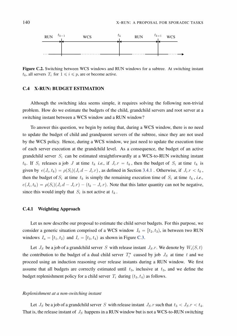
140 X-RUN: A PROPOSAL FOR SPORADIC TASKS
RUN tk´1 WCS tk RUN tk`1 WCS
Figure C.2. Switching between WCS windows and RUN windows for a subtree. At switching instanttk, all servers Ti for 1 ď i ď p, are or become active.
C.4 X-RUN: BUDGET ESTIMATION
Although the switching idea seems simple, it requires solving the following non-trivial
problem. How do we estimate the budgets of the child, grandchild servers and root server at a
switching instant between a WCS window and a RUN window?
To answer this question, we begin by noting that, during a WCS window, there is no need
to update the budget of child and grandparent servers of the subtree, since they are not used
by the WCS policy. Hence, during a WCS window, we just need to update the execution time
of each server execution at the grandchild level. As a consequence, the budget of an active
grandchild server Si can be estimated straightforwardly at a WCS-to-RUN switching instant
tk. If Si releases a job J at time tk i.e., if Ji.r “ tk , then the budget of Si at time tk is
given by epJi, tkq “ ρpSiqpJi.d ´ Ji.rq , as defined in Section 3.4.1 . Otherwise, if Ji.r ă tk ,
then the budget ofSi at time tk is simply the remaining execution time of Si at time tk , i.e.,
epJi, tkq “ ρpSiqpJi.d ´ Ji.rq ´ ptk ´ Ji.rq. Note that this latter quantity can not be negative,
since this would imply that Si is not active at tk .
C.4.1 Weighting Approach
Let us now describe our proposal to estimate the child server budgets. For this purpose, we
consider a generic situation comprised of a WCS window Ib “ rt2, t3q, in between two RUN
windows Ia “ rt1, t2q and Ic “ rt3, t4q as shown in Figure C.3.
Let JS be a job of a grandchild server S with release instant JS.r. We denote by WipS, tq
the contribution to the budget of a dual child server T ˚i caused by job JS at time t and we
proceed using an induction reasoning over release instants during a RUN window. We first
assume that all budgets are correctly estimated until t3, inclusive at t3, and we define the
budget replenishment policy for a child server Ti during pt3, t4q as follows.
Replenishment at a non-switching instant
Let JS be a job of a grandchild server S with release instant JS.r such that t3 ă JS.r ă t4.
That is, the release instant of JS happens in a RUN window but is not a WCS-to-RUN switching
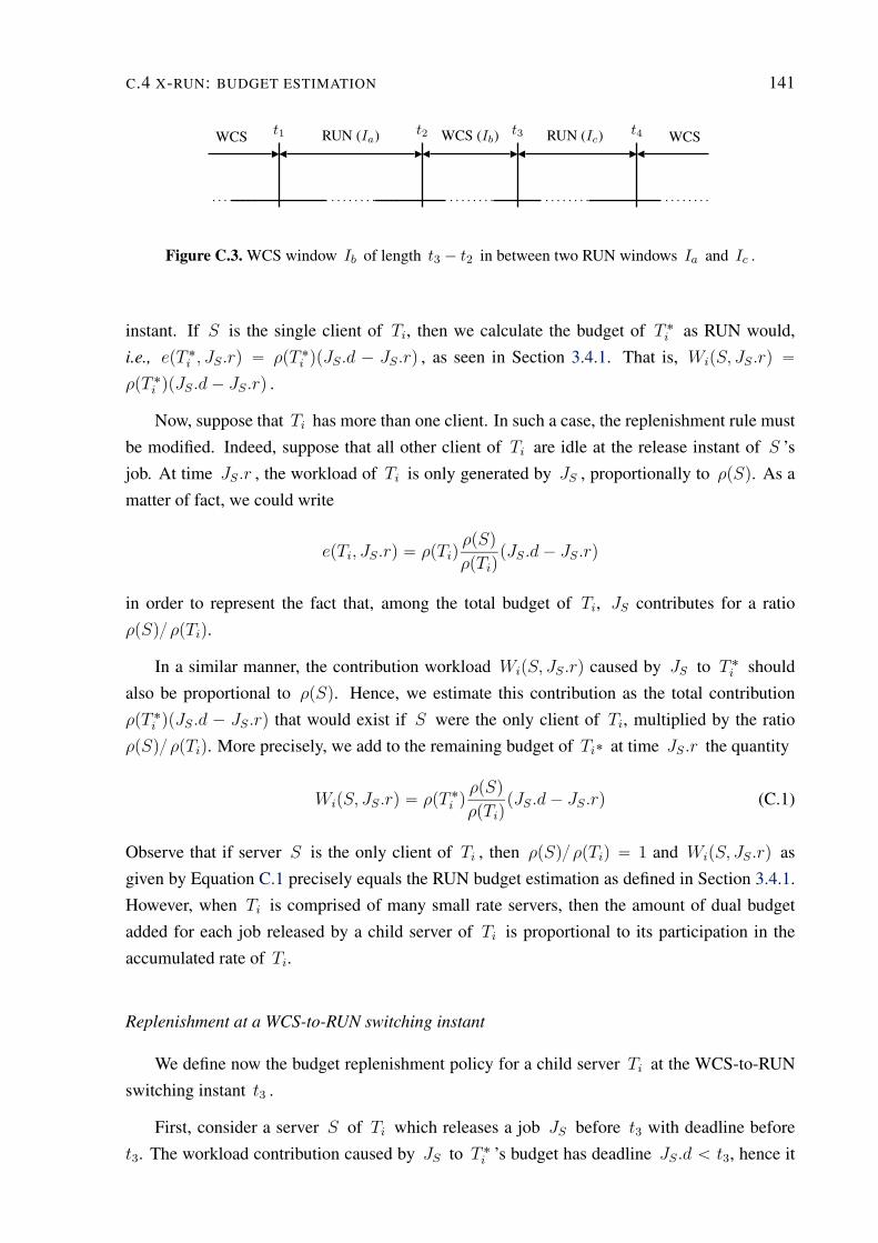
C.4 X-RUN: BUDGET ESTIMATION 141
WCS t1 RUN (Ia) t2 WCS (Ib) t3 RUN (Ic) t4 WCS
Figure C.3. WCS window Ib of length t3 ´ t2 in between two RUN windows Ia and Ic .
instant. If S is the single client of Ti, then we calculate the budget of T ˚i as RUN would,
i.e., epT ˚i , JS.rq “ ρpT ˚
i qpJS.d ´ JS.rq , as seen in Section 3.4.1. That is, WipS, JS.rq “
ρpT ˚i qpJS.d ´ JS.rq .
Now, suppose that Ti has more than one client. In such a case, the replenishment rule must
be modified. Indeed, suppose that all other client of Ti are idle at the release instant of S ’s
job. At time JS.r , the workload of Ti is only generated by JS , proportionally to ρpSq. As a
matter of fact, we could write
epTi, JS.rq “ ρpTiqρpSq
ρpTiqpJS.d ´ JS.rq
in order to represent the fact that, among the total budget of Ti, JS contributes for a ratio
ρpSq ρpTiq.
In a similar manner, the contribution workload WipS, JS.rq caused by JS to T ˚i should
also be proportional to ρpSq. Hence, we estimate this contribution as the total contribution
ρpT ˚i qpJS.d ´ JS.rq that would exist if S were the only client of Ti, multiplied by the ratio
ρpSq ρpTiq. More precisely, we add to the remaining budget of Ti˚ at time JS.r the quantity
WipS, JS.rq “ ρpT ˚i qρpSq
ρpTiqpJS.d ´ JS.rq (C.1)
Observe that if server S is the only client of Ti , then ρpSq ρpTiq “ 1 and WipS, JS.rq as
given by Equation C.1 precisely equals the RUN budget estimation as defined in Section 3.4.1.
However, when Ti is comprised of many small rate servers, then the amount of dual budget
added for each job released by a child server of Ti is proportional to its participation in the
accumulated rate of Ti.
Replenishment at a WCS-to-RUN switching instant
We define now the budget replenishment policy for a child server Ti at the WCS-to-RUN
switching instant t3 .
First, consider a server S of Ti which releases a job JS before t3 with deadline before
t3. The workload contribution caused by JS to T ˚i ’s budget has deadline JS.d ă t3, hence it
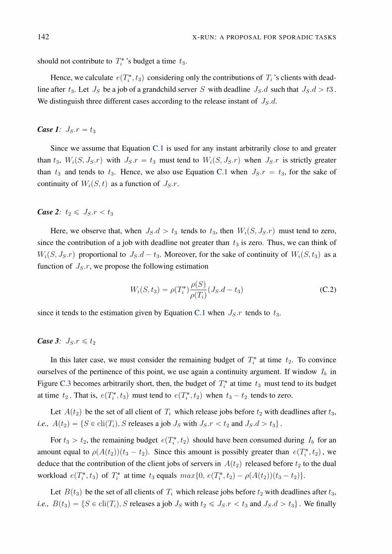
142 X-RUN: A PROPOSAL FOR SPORADIC TASKS
should not contribute to T ˚i ’s budget a time t3.
Hence, we calculate epT ˚i , t3q considering only the contributions of Ti ’s clients with dead-
line after t3. Let JS be a job of a grandchild server S with deadline JS.d such that JS.d ą t3 .
We distinguish three different cases according to the release instant of JS.d.
Case 1: JS.r “ t3
Since we assume that Equation C.1 is used for any instant arbitrarily close to and greater
than t3, WipS, JS.rq with JS.r “ t3 must tend to WipS, JS.rq when JS.r is strictly greater
than t3 and tends to t3. Hence, we also use Equation C.1 when JS.r “ t3, for the sake of
continuity of WipS, tq as a function of JS.r.
Case 2: t2 ď JS.r ă t3
Here, we observe that, when JS.d ą t3 tends to t3, then WipS, JS.rq must tend to zero,
since the contribution of a job with deadline not greater than t3 is zero. Thus, we can think of
WipS, JS.rq proportional to JS.d ´ t3. Moreover, for the sake of continuity of WipS, t3q as a
function of JS.r, we propose the following estimation
WipS, t3q “ ρpT ˚i qρpSq
ρpTiqpJS.d ´ t3q (C.2)
since it tends to the estimation given by Equation C.1 when JS.r tends to t3.
Case 3: JS.r ď t2
In this later case, we must consider the remaining budget of T ˚i at time t2. To convince
ourselves of the pertinence of this point, we use again a continuity argument. If window Ib in
Figure C.3 becomes arbitrarily short, then, the budget of T ˚i at time t3 must tend to its budget
at time t2 . That is, epT ˚i , t3q must tend to epT ˚
i , t2q when t3 ´ t2 tends to zero.
Let Apt2q be the set of all client of Ti which release jobs before t2 with deadlines after t3,
i.e., Apt2q “ tS P clipTiq, S releases a job JS with JS.r ă t2 and JS.d ą t3u .
For t3 ą t2, the remaining budget epT ˚i , t2q should have been consumed during Ib for an
amount equal to ρpApt2qqpt3 ´ t2q. Since this amount is possibly greater than epT ˚i , t2q , we
deduce that the contribution of the client jobs of servers in Apt2q released before t2 to the dual
workload epT ˚i , t3q of T ˚
i at time t3 equals maxt0, epT ˚i , t2q ´ ρpApt2qqpt3 ´ t2qu.
Let Bpt3q be the set of all clients of Ti which release jobs before t2 with deadlines after t3,
i.e., Bpt3q “ tS P clipTiq, S releases a job JS with t2 ď JS.r ă t3 and JS.d ą t3u . We finally
C.4 X-RUN: BUDGET ESTIMATION 143
obtain the following proposal for the estimation of T ˚i ’s budget at the WCS-to-RUN switching
instant t3:
epT ˚i , t3q “ maxtepT ˚
i , t2q ´ ρpApt2qqpt3 ´ t2qu `ÿ
SPBpt3q
WipS, t3q
“ maxtepT ˚i , t2q ´ ρpApt2qqpt3 ´ t2qu `
ÿ
SPBpt3q
ρpT ˚i qρpSq
ρpTiqpJS.d ´ t3q
C.4.2 Horizon Approach
In order to complete the picture of our proposal for the X-RUN algorithm, we must establish
the replenishment policy for the root server of a subtree.
For this purpose, we define the horizon hpU˚, tq of a root server U˚ of a subtree as the
earliest possible deadline among the jobs already active at time t or yet to be released after t.
Indeed, a grandchild server S , idle at time t , can release a job JS at any time after t . Then,
at time JS.r, the deadline JS.d would become the earliest deadline in the system. Thus, if
the budget of the root server U˚ had been estimated at time t using only the earliest inherited
deadline from the active servers at time t, then, at time JS.r, the earlier deadline JS.d would
decrease the U˚’s budget. Moreover, the budget estimated at time t could have been already
consumed at time JS.r, resulting in a possibly negative budget of U˚.
We prevent such event to happen by only replenishing the budget of root server U˚ until its
horizon, i.e.,, at a replenishment instant of U˚, we estimate its budget
epU˚, tq “ ρpU˚qphpU˚, tq ´ tq
Also, the next replenishment instants of U˚ after t is the earliest instant between hpU˚, tq
and the next release instant of a U˚ ’s grandchild job.
This last equation completes what we think that RUN must look like in order to cope with
the STID model. As mentioned before, this piece of work must still be and implemented and
proved correct.