Monte Carlo Localization for Robocup 3D Soccer Simulation League

Luis AguiarElectronic Engineering Division

Aeronautics Institute of TechnologyPraça Marechal Eduardo Gomes, 50

Vila das Acácias, 12228-900São José dos Campos, SP, Brazil

Email: luis.guilherme@aluno.ita.br

Marcos MáximoComputer Science Division

Aeronautics Institute of TechnologyPraça Marechal Eduardo Gomes, 50

Vila das Acácias, 12228-900São José dos Campos, SP, Brazil

Email: mmaximo@ita.br

Samuel PintoElectronic Engineering Division

Aeronautics Institute of TechnologyPraça Marechal Eduardo Gomes, 50

Vila das Acácias, 12228-900São José dos Campos, SP, Brazil

Email: sacepi@gmail.com

Abstract—This paper presents the application of the localiza-tion technique known as Monte Carlo Localization for theestimation of the global pose of virtual robots agents in theRobocup 3D Soccer Simulation League. It includes the overalltheoretical background concerning this filtering algorithm, thestochastic modeling for this localization problem, an overviewof this method’s implementation, simulation results and per-formance evaluation.

1. Introduction

Mobile robots have been recently accomplishing greattechnological advancements and visibility due to their widerange of applications in the real world. Latest efforts con-cerning humanoid robotics, one of the forefronts of roboticsresearch, include the necessity for the robot to interact withthe environment and therefore self-localize precisely. Thetask of estimating the robot’s global position and orientationusing its movement commands and sensor information iscalled localization, and that field has been proving to havegreat importance for performing sophisticated strategies anddecision making algorithms in humanoid soccer.

RoboCup Soccer 3D Simulation League is a particularlyinteresting challenge concerning humanoid robot soccer. Itconsists of a simulation environment of a soccer match withtwo teams, each one composed by up to 11 simulated NAORobots from Aldebaran Robotics, the official robot used forRoboCup Standard Platform League since 2008. RoboCupSoccer 3D competition allows the possibility for great en-hancements in the design and implementation of multi-agenthigh-level behaviors at the same time it provides a solidlow level platform for a realistic physical simulation of thegame. Hence, through this combination, it is a opportunityto research, implement and test advanced algorithms in therobot soccer challenge before moving to the next step andapply these techniques in real robots.

This work is based on the the development of a localiza-tion system for the team ITAndroids Soccer3D. ITAndroidsis a robotics research group at Technological Institute ofAeronautics which was refounded in mid-2011 after yearsof inactivity. To motivate the research, the group participates

in national and international competitions of RoboCup’sSoccer 2D, Soccer 3D and Humanoid Kid Size Leagues, asalso of IEEE’s Humanoid Robot Racing and IEEE’s VerySmall Size Soccer (VSS) categories. ITAndroids Soccer3Dteam has achieved some significant results in latest editionsof RoboCup (top 12 in 2013 and 2015) and Latin AmericaRobotics Competition (LARC) (1st place in 2012; 2nd placein 2013, 2014 and 2015).

For approaching this localization problem for this com-petition, it was used an extensively widespread probabilistictechnique called Monte Carlo Localization. This technique,known for a good estimation performance, draw particleswhich represent the posterior non-parametric distribution ofthe global agent pose. This model merges the informationfrom the robot’s locomotion with sensor measurements, andparticularly, in this case, sensoring is based on landmarksobservations. Moreover, the localization needs to deal withSoccer 3D’s simulator frequently teleporting the agent whencertain situations occur, which is an instance of the problemknown as robot kidnapping

The purpose of this paper is to present the imple-mentation of the mentioned localization technique in thedescribed problem, as well as assessing its performancebased on the Root Square Error (RSE), calculated duringthe simulation, and the computational time. In this work,Section 1 gives a presentation and overview of the problem,Section 2 describes the applied algorithm with some the-oretical background and Section 3 provides the stochasticmodel of the RoboCup Soccer 3D problem. In Section 4follows some simulation results, in Section 5 we can seethe main conclusions, future works and final considerations,and finally, Section 6 presents the people and entities whocontributed to this work.

2. Probabilistic Localization

The key idea about localization from a probabilisticapproach is representing robot’s pose xt at time step t by itsprobability distribution function (pdf) throughout the space,and by using mathematical techniques it is possible to reachgreater precision in estimating robot’s real position. The

probabilistic problem is usually modeled as a first orderMarkov Chain as described below:

xt+1 = f(xt, εt) + ut (1)

zt = h(xt) + vt (2)

Equation (1) represents the movement model of ouragent, where f is its propagation function, εk is the controlinput and ut a random noise associated with the process. Atthe same time, equation (2) is the measurement model ofthe system, given sensor observation zt and another additiverandom noise associated vt.

Our purpose, therefore, is to inductively merge thesemodels and obtain a final pose xt, given by the pdfp(xt|z1:t). The approach is through sample representation,exploiting the duality between the distribution functionand random samples generated by it. In particle filter,the algorithm used in this work, these samples are calledparticles, being of the same nature of the robot’s state.Xt := x

[1]t , x

[2]t , ..., x

[M ]t .

Algorithm 1 Monte Carlo Localization, derived from [[1]p.252][ [2]p.10]

1: Initialization2: Draw x

[m]0 ∼ p(x0),m = 1, . . . ,M

3: w[m]0 ← p(z0|x0)

4: w[m]0 ← w

[m]0∑M

m=0 w[m]0

5: X0 ← X0 ∪ 〈x[m]0 , w

[m]0 〉

6: function PARTICLE FILTER(Xt−1, zt)7: Xt = Xt ← ∅8: for m = 1 to M do9: draw x

[m]t ∼ p(xt|x[m]

t−1)

10: calculate w[m]t ←∝ p(zt|x[m]

t )

11: Xt ← Xt ∪ 〈x[m]t , w

[m]t 〉

12: end for13: Xt ← RESAMPLE(Xt)14: x̂t ← 1

M

∑Mm=0 x

[m]t

15: return x̂t, Xt

16: end function

As can be also seen in [1] and in [3], the overall ideaabout the algorithm follows other traditional techniques. Weassume that the particle set Xt−1 represents the previousiteration distribution, then we draw new particles fromthe previous one sampling from the importance functionp(xt|x[m]

t−1). This step is called prediction phase, as youcan predict the actual position based on the motion model,however it is corrupted by the random process noise and ina long term prediction-only simulation, the estimation tendsto run away from the real position.

In order to control this natural error, the key pointof the technique is approximating a specific distributionsampling from another distribution, since the intended finalpdf p(xt|z1:t) is originally unknown. Thus, starting from theset of particles Xt, distributed according to the importance

function p(xt|x[m]t−1), if we introduce the weight w[m]

t as inEq. (3), given by the ratio of the two distribution functionsin x[m]

t , Eq. (4) holds, where the function g(x) can be anymeasurable function.

w[m]t =

p(x[m]t |z1:t)

p(x[m]t |x

[m]t−1)

(3)

[M∑m=1

w[m]t

]−1 M∑m=1

g(x[m]t )w

[m]t

M→∞−−−−→∫A

g(xt)p(xt|z1:t) dxt

(4)In other words, it is possible to calculate any expectancy

over the posterior distribution in any given area A throughthe particles from the prediction phase, as long as we haveenough particles. Moreover, can be proven that w[m]

t can begiven in a calculable form, present in (5). This step is calledfiltering phase, as the target function reaches the desirabledistribution with estimate closer to the robot’s real position.

w[m]t =

w[m]t−1p(zt|x

[m]t )∑M

m=1 w[m]t

(5)

In the resample step we draw, from the predict set ofparticles, M particles according to each weight and allowingrepetition, compounding the final set Xt. The purpose isto decrease particles’ variance, reducing the number ofparticles with low weight too far from the actual position,otherwise it would be necessary many more particles toreach the same approximation performance. Since this pro-cedure incorporates the weights into the sampling process,it changes the particles distribution to the desired posteriorone. The weights can be reseted to 1

M , and the final poseestimate can be computed by the average of particles posi-tions.

The resample algorithm used can be found in [1] andin [4] and it’s advantage is the fact that, instead of inde-pendently resampling, the algorithm consists of a sequentialstochastic process, covering all the particle space and sortingparticles according to a single random number. The mainadvantage of this resampling algorithm is its computationalcomplexity of O(M), essential for a practical performanceand the computational viability of the particle filter.

Despite self-localizing properly, Algorithm (1) is limiteddealing with practical issues, such as false positives, sensorerrors and the eventual lost of the robot, in the case of thekidnapping problem. As proposed in [1](p. 256-261) and in[5], an augmented Monte Carlo Localization (Algorithm 2)is able to deal with these restrictions.

The main idea is to compute experimentally the observa-tion likelihood and store short-term and long-term values ofthis probability. It can be made by the parameters αslow andαfast, where αslow << αfast, which represent the decayrates for calculating the observation qualities. Then, eachparticle is resetted with probability max(0.0, 1.0 − wfast

wslow),

suggesting that if the short-term observation quality is worsethan the long-term one, particles must be resetted accordingto this difference, otherwise no further action is needed.

Algorithm 2 Augmented Monte Carlo Localization1: Initialization2: draw uniform particles3: wslow = wfast ← −1.0, w

[m]t ← 1/M,∀m

4: X0 ← X0 ∪ 〈x[m]0 , w

[m]0 〉

5: function UPDATE(Xt−1, Zt, wslow, wfast)6: wobs ← 0, Xt = Xt = ∅7: for m = 1 to M do8: x

[m]t ∼ p(x[m]

t |x[m]t−1)

9: pobs ← p(Zt, x[m]t )

10: wobs ← wobs + pobs11: w

[m]t ← w

[m]t−1pobs

12: end for13: w

[m]t ← w

[m]t∑M

m=0 w[m]t

14: Xt ← Xt ∪ 〈x[m]t , w

[m]t 〉,∀m

15: wslow ← (1− αslow)wslow + αslowwobs16: wfast ← (1− αfast)wfast + αfastwobs17: preset ← MAX(0.0, 1.0− wfast

wslow)

18: Xt ← RESAMPLE(Xt)19: for m = 1 to M do20: if RANDOM() < preset then21: (z1, z2)←SAMPLETWOLANDMARKS(Zt)22: SENSORPARTICLERESET(z1, z2, x

[m]t )

23: end if24: end for25: x̂t ← 1

M

∑Mm=0 x

[m]t

26: return x̂t, Xt, wslow, wfast27: end function

That action implies that, when occurring a big shift inthe measurement likelihood, is better to change particleslocation based on sensor information solely (see [6]) thancontinuously losing particles variety in the resample step.Moreover, the smoothed calculation of wfast and wslowreduce the error caused by false positives and momentarysensor failures (see Algorithm 2).

3. Stochastic Modeling for 3D Soccer Simula-tion

In RoboCup 3D Soccer Simulation, for the global lo-calization problem, the robot’s pose is given by its twodimensional coordinates in the field, x e y, and by thehorizontal angle its torso is heading, therefore, it is of theform x

[m]t = [x, y, ψ].

The motion model is given by the information providedby the walking engine in the control layer, in the formof 3-dimensional displacement of the center of the torso,given in the local torso coordinates frame of the previousiteration. In that way, locomotion information is a vector∆dt = [∆xt,∆yt,∆ψt]. However, it presents a significantdifference from the real movement due to slip, mostly inhigh speed circumstances. For solving this issue, we multi-ply each element of the vector ∆dt by a constant parameter,as can be seen in 6.

d′t =

∆x′t∆y′t∆ψ′t

=

α∆xtβ∆ytγ∆ψt

(6)

This new vector represents the actual displacement usedin the movement model, the parameters α, β and γ weremanually tuned comparing the real position evolution andits estimation through the walk algorithm. Therefore, wereach the following model for the position update of eachparticle.

x[m]t

y[m]t

ψ[m]t

=

x[m]t−1 + ∆x′tcos(ψt−1)−∆y′tsin(ψt−1)

y[m]t−1 + ∆x′tsin(ψt−1) + ∆y′tcos(ψt−1)

ψ[m]t−1 + ∆ψ′t

+

uxuyuψ

(7)

Where ux ∼ N(0, σ2x), uy ∼ N(0, σ2

y) and uψ ∼N(0, σ2

ψ) are Gaussian noises associated with the process.The values σ2

x, σ2y and σ2

ψ were also manually tweakedcomparing the real evolution and the predict one.

The observation model is given by landmarks detections(flags and goal posts). In Robocup Soccer 3D, this infor-mation is provided by the server in the form of perceptors,strings which contain the distance to the center of the objectsdescribed as a vector in spherical coordinates, which is the3-dimensional distance and also the horizontal and latitudi-nal angle in relation to the camera. In the perception layer,this information is decodified and the distances passed fromthe camera’s referential to the same two-dimensional systemof the robot’s pose, thus giving the horizontal distance andbearing angle from the object. The perceptors documentationcan be found in [7].

Landmarks observations are also corrupted by Gaussiannoise, in both horizontal distance and angle, described by thevariances σ2

d and σ2ψ. We also assume that these measure-

ments, and also from different landmarks, are independent ofeach other. Therefore, a suitable rule for updating particles’weights follows in (8).

w[m]t = w

[m]t−1

∏j

exp

[− (dj − d̂j

[m])2

2σ2d

]exp

[− (ψj − ψ̂j

[m])2

2σ2ψ

](8)

In this model, dj and ψj are the measured horizontaldistance and horizontal angle between the robot and the j-thlandmark, and d̂j

[m]and ψ̂j

[m]are the calculated expected

horizontal distance and horizontal angle between the j-thlandmark and the robot in the m-th particle position. Again,the variances were determined empirically, starting from thegiven ones in Simspark’s documentation [7], these valueswere manually tuned comparing the measurement predictionand the real model.

Note that weights update, and therefore the resample andparticles reset steps, are only performed when vision updateis detected. Data from vision is reported by the server every3 simulation cycles (0.06 sec), meanwhile the estimationprocess consider only the update from the motion model,happening each cycle.

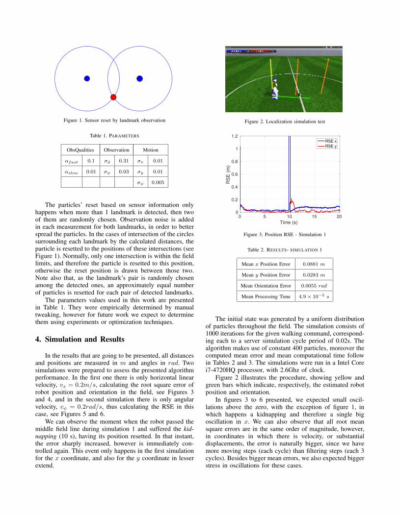
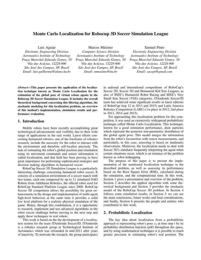
Figure 1. Sensor reset by landmark observation

Table 1. PARAMETERS

ObsQualities Observation Motion

αfast 0.1 σd 0.31 σx 0.01

αslow 0.01 σψ 0.03 σy 0.01

σψ 0.005

The particles’ reset based on sensor information onlyhappens when more than 1 landmark is detected, then twoof them are randomly chosen. Observation noise is addedin each measurement for both landmarks, in order to betterspread the particles. In the cases of intersection of the circlessurrounding each landmark by the calculated distances, theparticle is resetted to the positions of these intersections (seeFigure 1). Normally, only one intersection is within the fieldlimits, and therefore the particle is resetted to this position,otherwise the reset position is drawn between those two.Note also that, as the landmark’s pair is randomly chosenamong the detected ones, an approximately equal numberof particles is resetted for each pair of detected landmarks.

The parameters values used in this work are presentedin Table 1. They were empirically determined by manualtweaking, however for future work we expect to determinethem using experiments or optimization techniques.

4. Simulation and Results

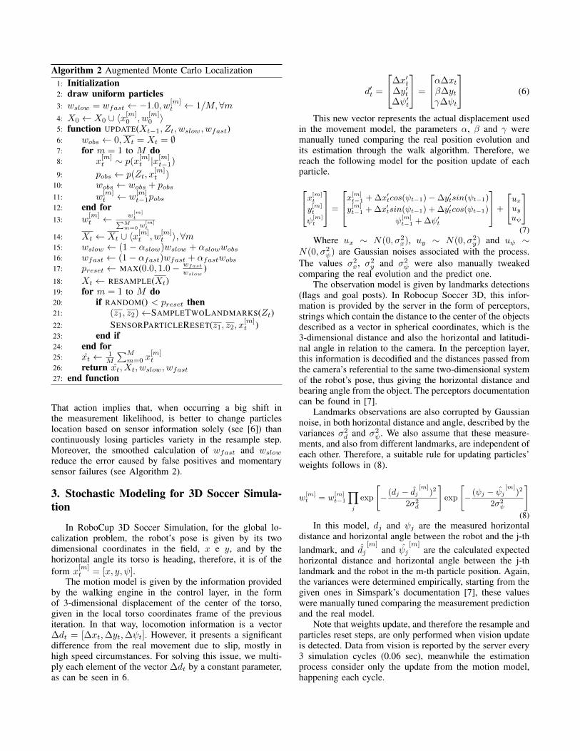
In the results that are going to be presented, all distancesand positions are measured in m and angles in rad. Twosimulations were prepared to assess the presented algorithmperformance. In the first one there is only horizontal linearvelocity, vx = 0.2m/s, calculating the root square error ofrobot position and orientation in the field, see Figures 3and 4, and in the second simulation there is only angularvelocity, vψ = 0.2rad/s, thus calculating the RSE in thiscase, see Figures 5 and 6.

We can observe the moment when the robot passed themiddle field line during simulation 1 and suffered the kid-napping (10 s), having its position resetted. In that instant,the error sharply increased, however is immediately con-trolled again. This event only happens in the first simulationfor the x coordinate, and also for the y coordinate in lesserextend.

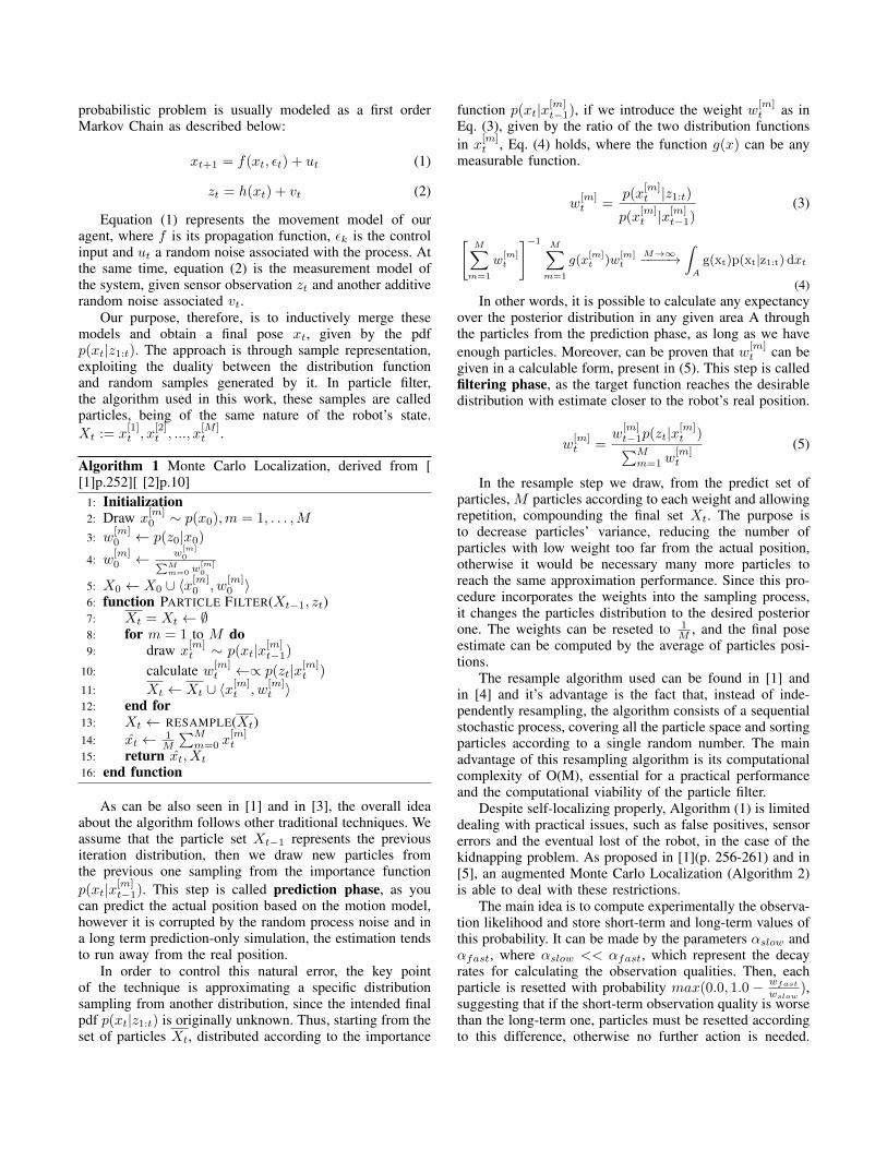
Figure 2. Localization simulation test

0 5 10 15 20

Time (s)

0

0.2

0.4

0.6

0.8

1

1.2

RS

E (

m)

RSE x

RSE y

Figure 3. Position RSE - Simulation 1

Table 2. RESULTS- SIMULATION 1

Mean x Position Error 0.0881 m

Mean y Position Error 0.0283 m

Mean Orientation Error 0.0055 rad

Mean Processing Time 4.9× 10−5 s

The initial state was generated by a uniform distributionof particles throughout the field. The simulation consists of1000 iterations for the given walking command, correspond-ing each to a server simulation cycle period of 0.02s. Thealgorithm makes use of constant 400 particles, moreover thecomputed mean error and mean computational time followin Tables 2 and 3. The simulations were run in a Intel Corei7-4720HQ processor, with 2.6Ghz of clock.

Figure 2 illustrates the procedure, showing yellow andgreen bars which indicate, respectively, the estimated robotposition and orientation.

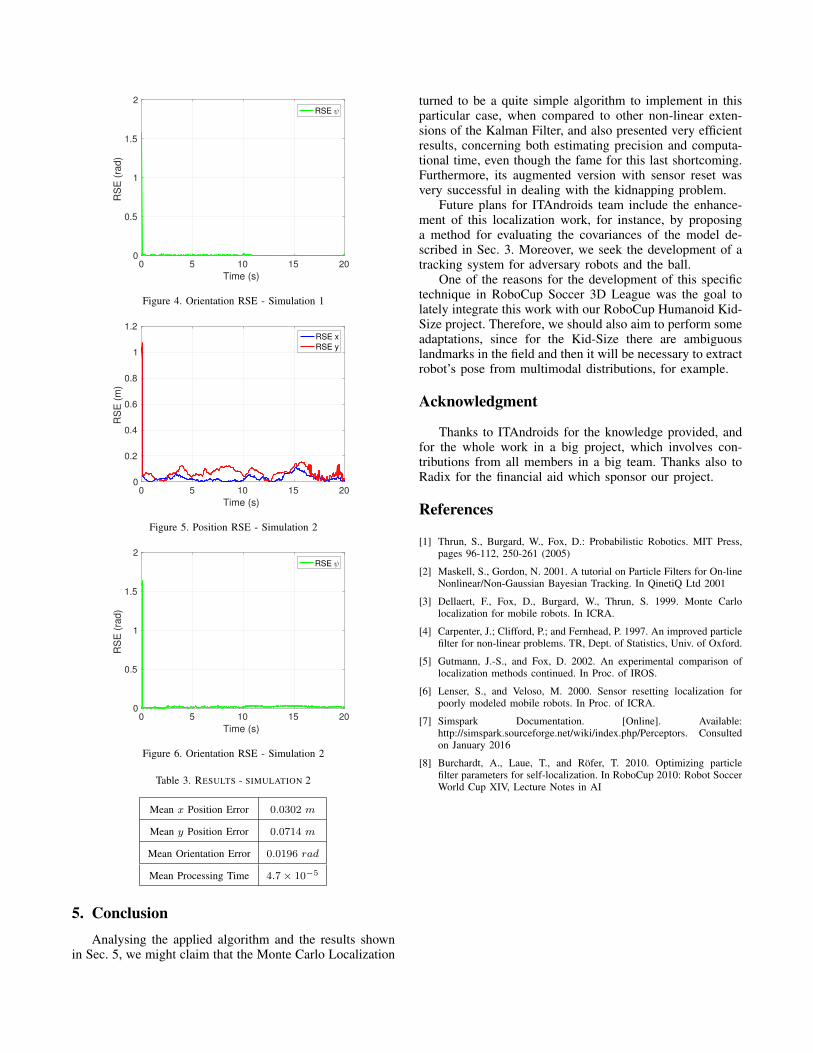
In figures 3 to 6 presented, we expected small oscil-lations above the zero, with the exception of figure 1, inwhich happens a kidnapping and therefore a single bigoscillation in x. We can also observe that all root meansquare errors are in the same order of magnitude, however,in coordinates in which there is velocity, or substantialdisplacements, the error is naturally bigger, since we havemore moving steps (each cycle) than filtering steps (each 3cycles). Besides bigger mean errors, we also expected biggerstress in oscillations for these cases.

0 5 10 15 20

Time (s)

0

0.5

1

1.5

2

RS

E (

rad

)RSE ψ

Figure 4. Orientation RSE - Simulation 1

0 5 10 15 20

Time (s)

0

0.2

0.4

0.6

0.8

1

1.2

RS

E (

m)

RSE x

RSE y

Figure 5. Position RSE - Simulation 2

0 5 10 15 20

Time (s)

0

0.5

1

1.5

2

RS

E (

rad

)

RSE ψ

Figure 6. Orientation RSE - Simulation 2

Table 3. RESULTS - SIMULATION 2

Mean x Position Error 0.0302 m

Mean y Position Error 0.0714 m

Mean Orientation Error 0.0196 rad

Mean Processing Time 4.7× 10−5

5. ConclusionAnalysing the applied algorithm and the results shown

in Sec. 5, we might claim that the Monte Carlo Localization

turned to be a quite simple algorithm to implement in thisparticular case, when compared to other non-linear exten-sions of the Kalman Filter, and also presented very efficientresults, concerning both estimating precision and computa-tional time, even though the fame for this last shortcoming.Furthermore, its augmented version with sensor reset wasvery successful in dealing with the kidnapping problem.

Future plans for ITAndroids team include the enhance-ment of this localization work, for instance, by proposinga method for evaluating the covariances of the model de-scribed in Sec. 3. Moreover, we seek the development of atracking system for adversary robots and the ball.

One of the reasons for the development of this specifictechnique in RoboCup Soccer 3D League was the goal tolately integrate this work with our RoboCup Humanoid Kid-Size project. Therefore, we should also aim to perform someadaptations, since for the Kid-Size there are ambiguouslandmarks in the field and then it will be necessary to extractrobot’s pose from multimodal distributions, for example.

Acknowledgment

Thanks to ITAndroids for the knowledge provided, andfor the whole work in a big project, which involves con-tributions from all members in a big team. Thanks also toRadix for the financial aid which sponsor our project.

References

[1] Thrun, S., Burgard, W., Fox, D.: Probabilistic Robotics. MIT Press,pages 96-112, 250-261 (2005)

[2] Maskell, S., Gordon, N. 2001. A tutorial on Particle Filters for On-lineNonlinear/Non-Gaussian Bayesian Tracking. In QinetiQ Ltd 2001

[3] Dellaert, F., Fox, D., Burgard, W., Thrun, S. 1999. Monte Carlolocalization for mobile robots. In ICRA.

[4] Carpenter, J.; Clifford, P.; and Fernhead, P. 1997. An improved particlefilter for non-linear problems. TR, Dept. of Statistics, Univ. of Oxford.

[5] Gutmann, J.-S., and Fox, D. 2002. An experimental comparison oflocalization methods continued. In Proc. of IROS.

[6] Lenser, S., and Veloso, M. 2000. Sensor resetting localization forpoorly modeled mobile robots. In Proc. of ICRA.

[7] Simspark Documentation. [Online]. Available:http://simspark.sourceforge.net/wiki/index.php/Perceptors. Consultedon January 2016

[8] Burchardt, A., Laue, T., and Röfer, T. 2010. Optimizing particlefilter parameters for self-localization. In RoboCup 2010: Robot SoccerWorld Cup XIV, Lecture Notes in AI