Universidade do MinhoEscola de EngenhariaDepartamento de Informatica

Marta Vasconcelos Castro Azevedo

Correct Translation of Imperative Programsto Single Assignment Form

January 2017

Universidade do MinhoEscola de EngenhariaDepartamento de Informatica

Marta Vasconcelos Castro Azevedo

Correct Translation of Imperative Programsto Single Assignment Form

Master dissertationMaster Degree in Computer Science

Dissertation supervised byProfessor Maria Joao FradeProfessor Luıs Pinto

January 2017

A B S T R AC T

A common practice in compiler design is to have an intermediate representation of the source code

in Static Single-Assignment (SSA) form in order to simplify the code optimization process and make

it more efficient. Generally, one says that an imperative program is in SSA form if each variable is

assigned exactly once.

In this thesis we study the central ideas of SSA-programs in the context of a simple imperative lan-

guage including jump instructions. The focus of this work is the proof of correctness of a translation

from programs of the source imperative language into the SSA format. In particular, we formally intro-

duce the syntax and the semantics of the source imperative language (GL ) and the SSA language; we

define and implement a function that translates from source imperative programs into SSA-programs;

we develop an alternative operational semantics, in order to be able to relate the execution of a source

program and of its SSA translation; we prove soundness and completeness results for the translation,

relatively to the alternative operational semantics, and from these results we prove correctness of the

translation relatively to the initial small-step semantics.

i

R E S U M O

Uma pratica comum no design de compiladores e ter uma representacao intermedia do codigo fonte

em formato Static Single Assigment (SSA), de modo a facilitar o processo subsequente de analise e

optimizacao de codigo. Em termos gerais, diz-se que um programa imperativo esta no formato SSA

se cada variavel do programa e atribuıda exatamente uma vez.

Nesta tese estudamos as ideias principais do SSA no contexto de uma linguagem imperativa simples

com instrucoes de salto. O foco deste trabalho e a prova de correccao de uma traducao dos programas

fonte para formato SSA. Concretamente, definimos formalmente a sintaxe e a semantica da linguagem

fonte (GL) e da linguagem em formato SSA; definimos e implementamos a funcao de traducao; desen-

volvemos semanticas operacionais alternativas de modo a permitir relacionar a execucao do programa

fonte com a sua traducao SSA; provamos a idoneidade e a completude do processo de traducao relati-

vamente as semanticas alternativas definidas; e a partir destes resultados demostramos a correccao da

traducao em ordem as semanticas operacionais estruturais definidas inicialmente.

ii

C O N T E N T S

1 I N T RO D U C T I O N 2

1.1 Imperative and functional programming 2

1.2 Compilation process 3

1.3 Single assignment form 4

1.4 Continuation passing style 6

1.5 Contributions and document structure 7

2 I M P E R AT I V E L A N G UAG E A N D S I N G L E A S S I G N M E N T F O R M 9

2.1 The Goto Language GL 9

2.1.1 Syntax 10

2.1.2 Semantics 12

2.2 SA language 15

2.2.1 Syntax 15

2.2.2 Operational semantics in SA programs 17

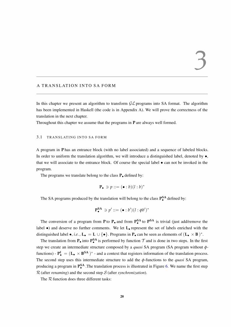
3 A T R A N S L AT I O N I N T O S A F O R M 20

3.1 Translating into SA form 20

4 C O R R E C T N E S S O F T H E T R A N S L AT I O N I N T O S A F O R M 27

4.1 Splitting the transition relation of the source language GL 27

4.1.1 Computation inside block 27

4.1.2 Computation across blocks 28

4.2 Splitting the transition relation in the SA language 31

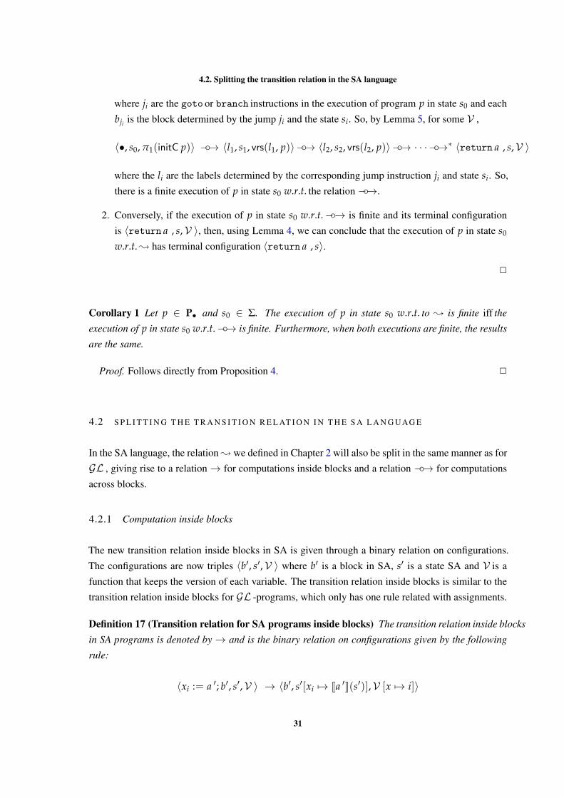
4.2.1 Computation inside blocks 31

4.2.2 Computation across blocks 32

4.3 Properties of the translation into SA form 35

4.3.1 Soundness 36

4.3.2 Completeness 40

4.3.3 Correctness 46

5 F I N A L R E M A R K S 48

5.1 SA Translation 48

5.1.1 Optimal placement of φ-functions 48

5.1.2 Adapting the translation function T 50

5.2 Relation with Functional Programming 52

5.3 Conclusions and Future Work 54

A A P P E N D I X 58

iii

Contents

B A P P E N D I X 65

iv

L I S T O F F I G U R E S

Figure 1 Example of a imperative program 3

Figure 2 Example of a functional program 3

Figure 3 Translation in a simple program in SA 4

Figure 4 Example of a transformation into SSA form 6

Figure 5 CFG corresponding to example presented in Figure 1 6

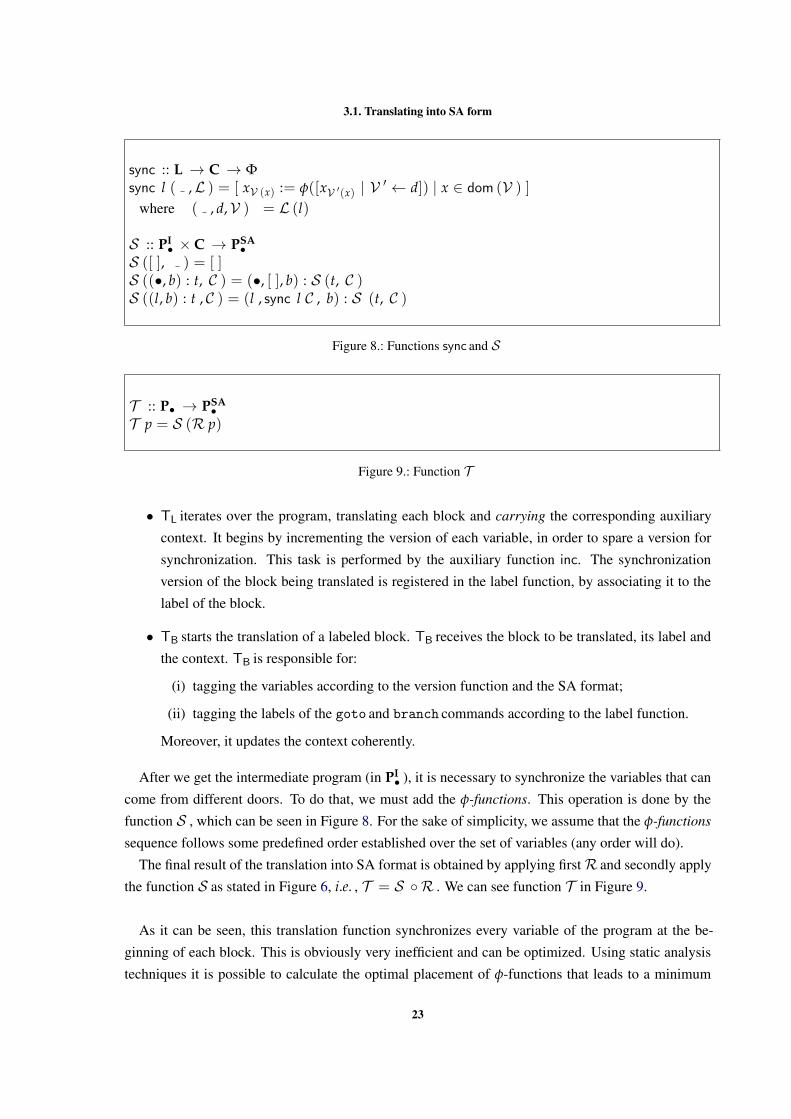
Figure 6 Translation into SA format 21

Figure 7 FunctionR and its auxiliary functions 22

Figure 8 Functions sync and S 23

Figure 9 Function T 23

Figure 10 Program sum and its CFG 49

Figure 11 Translation into SA format with OP 50

Figure 12 FunctionR and its auxiliary functions 51

Figure 13 Function S 51

Figure 14 Function T 52

Figure 15 The program sum and its translations with the two versions of T 53

v

L I S T O F A B B R E V I AT I O N S

CPS Continuation Passing Style

SA Single Assignment

SSA Static Single Assignment

CFG Control Flow Graph

1

1

I N T RO D U C T I O N

1.1 I M P E R AT I V E A N D F U N C T I O N A L P RO G R A M M I N G

A programming language is a notation for writing programs, which are specifications of a computation

to be performed by a machine. Different approaches to programming have been developed over

time. There are many different programming paradigms that allow the possibility to determine the

programmer’s view of the problem. Despite some languages are designed to support one particular

paradigm, there are others that support multiple paradigms.

This work focuses on two of these paradigms, which have drawn programmers and computer scien-

tists’ attention since early times: the imperative programming paradigm and the functional program-

ming paradigm. Both paradigms are built upon different ideas.

In imperative languages computation is specified in an imperative form (i.e., as a sequence of

operations to perform). The model of computation in the imperative paradigm relies on the notion of

state (seen as the content of the program variables which represent storage/memory locations, at any

given point in the program’s execution ) and statements/commands that change a program’s state. So,

an imperative program consists of a sequence of commands for the computer to perform. A program

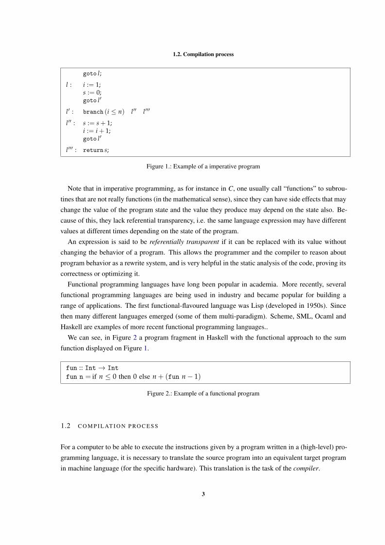
describes how a program operates. In Figure 1 we can see a snippet of a imperative program. This

program sums all the numbers from 0 to n.

The first imperative programming languages were machine languages with simple instructions.

Gradually, some more complex languages were introduced such as C, Pascal or Java.

Contrasting with imperative programming, functional programming focuses on what the program

should accomplish without specifying how the program should achieve the result. Functional program-

ming has its roots in λ-calculus (Church, 1932). The functional programming paradigm is based on

the notion of mathematical function (a program is a collection of functions) and program execution

corresponds to the evaluation of expressions (involving the functions defined in the program). Func-

tional programs deal only with mathematical variables (the formal arguments of the functions). The

output value of a function depends only on the arguments that are inputs to the function. So, calling a

function twice with the same argument values will produce the same result each time. This property

is called referential transparency and make it much easier to understand and predict the behavior of a

program.

2

1.2. Compilation process

goto l;

l : i := 1;s := 0;goto l′

l′ : branch (i ≤ n) l′′ l′′′

l′′ : s := s + 1;i := i + 1;goto l′

l′′′ : return s;

Figure 1.: Example of a imperative program

Note that in imperative programming, as for instance in C, one usually call “functions” to subrou-

tines that are not really functions (in the mathematical sense), since they can have side effects that may

change the value of the program state and the value they produce may depend on the state also. Be-

cause of this, they lack referential transparency, i.e. the same language expression may have different

values at different times depending on the state of the program.

An expression is said to be referentially transparent if it can be replaced with its value without

changing the behavior of a program. This allows the programmer and the compiler to reason about

program behavior as a rewrite system, and is very helpful in the static analysis of the code, proving its

correctness or optimizing it.

Functional programming languages have long been popular in academia. More recently, several

functional programming languages are being used in industry and became popular for building a

range of applications. The first functional-flavoured language was Lisp (developed in 1950s). Since

then many different languages emerged (some of them multi-paradigm). Scheme, SML, Ocaml and

Haskell are examples of more recent functional programming languages..

We can see, in Figure 2 a program fragment in Haskell with the functional approach to the sum

function displayed on Figure 1.

fun :: Int→ Int

fun n = if n ≤ 0 then 0 else n + (fun n− 1)

Figure 2.: Example of a functional program

1.2 C O M P I L AT I O N P RO C E S S

For a computer to be able to execute the instructions given by a program written in a (high-level) pro-

gramming language, it is necessary to translate the source program into an equivalent target program

in machine language (for the specific hardware). This translation is the task of the compiler.

3

1.3. Single assignment form

Original Program SA Program

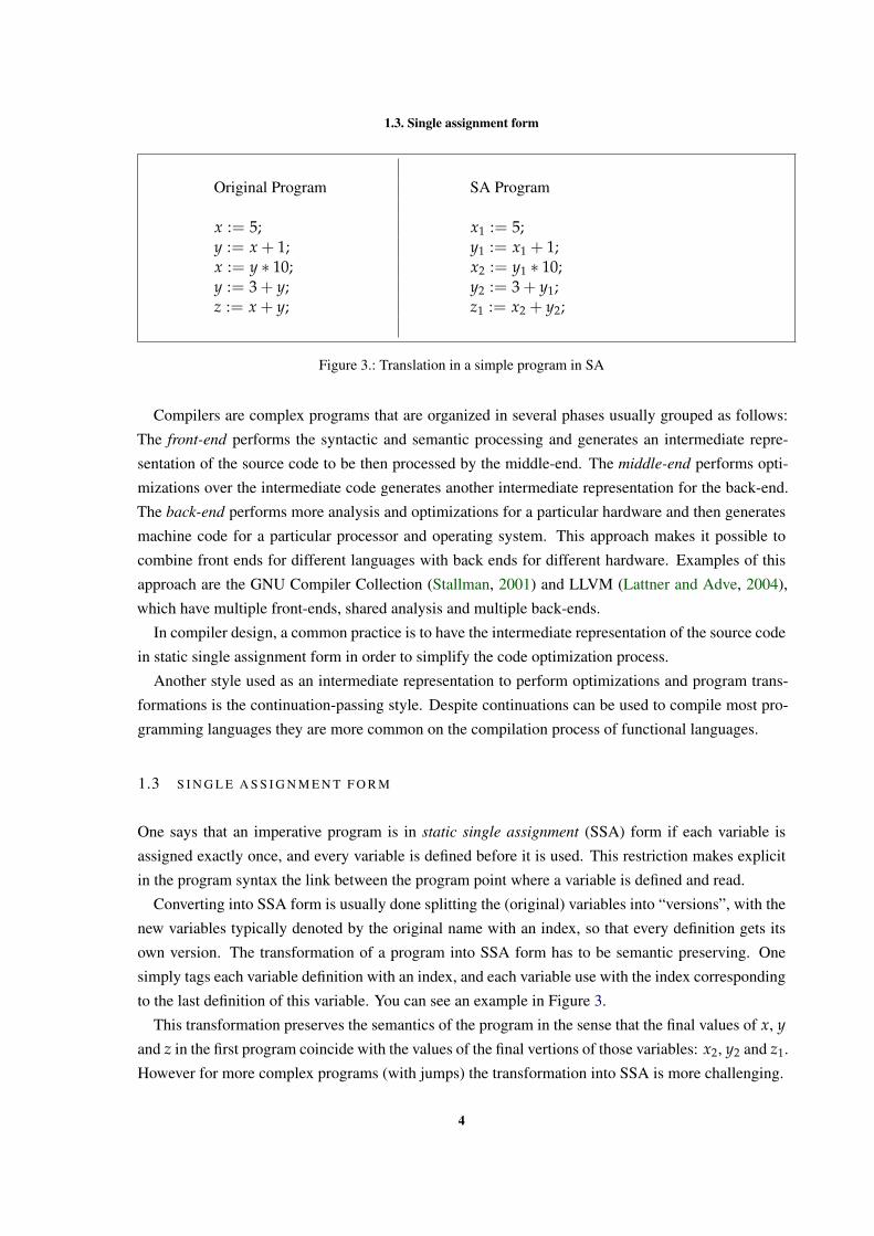
x := 5; x1 := 5;y := x + 1; y1 := x1 + 1;x := y ∗ 10; x2 := y1 ∗ 10;y := 3 + y; y2 := 3 + y1;z := x + y; z1 := x2 + y2;

Figure 3.: Translation in a simple program in SA

Compilers are complex programs that are organized in several phases usually grouped as follows:

The front-end performs the syntactic and semantic processing and generates an intermediate repre-

sentation of the source code to be then processed by the middle-end. The middle-end performs opti-

mizations over the intermediate code generates another intermediate representation for the back-end.

The back-end performs more analysis and optimizations for a particular hardware and then generates

machine code for a particular processor and operating system. This approach makes it possible to

combine front ends for different languages with back ends for different hardware. Examples of this

approach are the GNU Compiler Collection (Stallman, 2001) and LLVM (Lattner and Adve, 2004),

which have multiple front-ends, shared analysis and multiple back-ends.

In compiler design, a common practice is to have the intermediate representation of the source code

in static single assignment form in order to simplify the code optimization process.

Another style used as an intermediate representation to perform optimizations and program trans-

formations is the continuation-passing style. Despite continuations can be used to compile most pro-

gramming languages they are more common on the compilation process of functional languages.

1.3 S I N G L E A S S I G N M E N T F O R M

One says that an imperative program is in static single assignment (SSA) form if each variable is

assigned exactly once, and every variable is defined before it is used. This restriction makes explicit

in the program syntax the link between the program point where a variable is defined and read.

Converting into SSA form is usually done splitting the (original) variables into “versions”, with the

new variables typically denoted by the original name with an index, so that every definition gets its

own version. The transformation of a program into SSA form has to be semantic preserving. One

simply tags each variable definition with an index, and each variable use with the index corresponding

to the last definition of this variable. You can see an example in Figure 3.

This transformation preserves the semantics of the program in the sense that the final values of x, yand z in the first program coincide with the values of the final vertions of those variables: x2, y2 and z1.

However for more complex programs (with jumps) the transformation into SSA is more challenging.

4

1.3. Single assignment form

The SSA form was introduced in the 1980s by Ron Cytron et al (Cytron et al., 1991) and it is

a popular intermediate representation for compiler optimizations. The considerable strength of the

SSA form, where variables are statically assigned exactly once, simplifies the definition of many

optimizations, and improves their efficiency and the quality of their results. The SSA format plays

a central role in a range of optimization algorithms relying on data flow information, and hence,

to the correctness of compilers employing those algorithms. Examples of optimization algorithms

which benefit from the use of SSA form include, among others, constant propagation, value range

propagation, dead code elimination and register allocation. Many modern optimizing compilers, such

as the GNU Compiler Collection and LLVM Compiler Infrastructure rely heavily on SSA form.

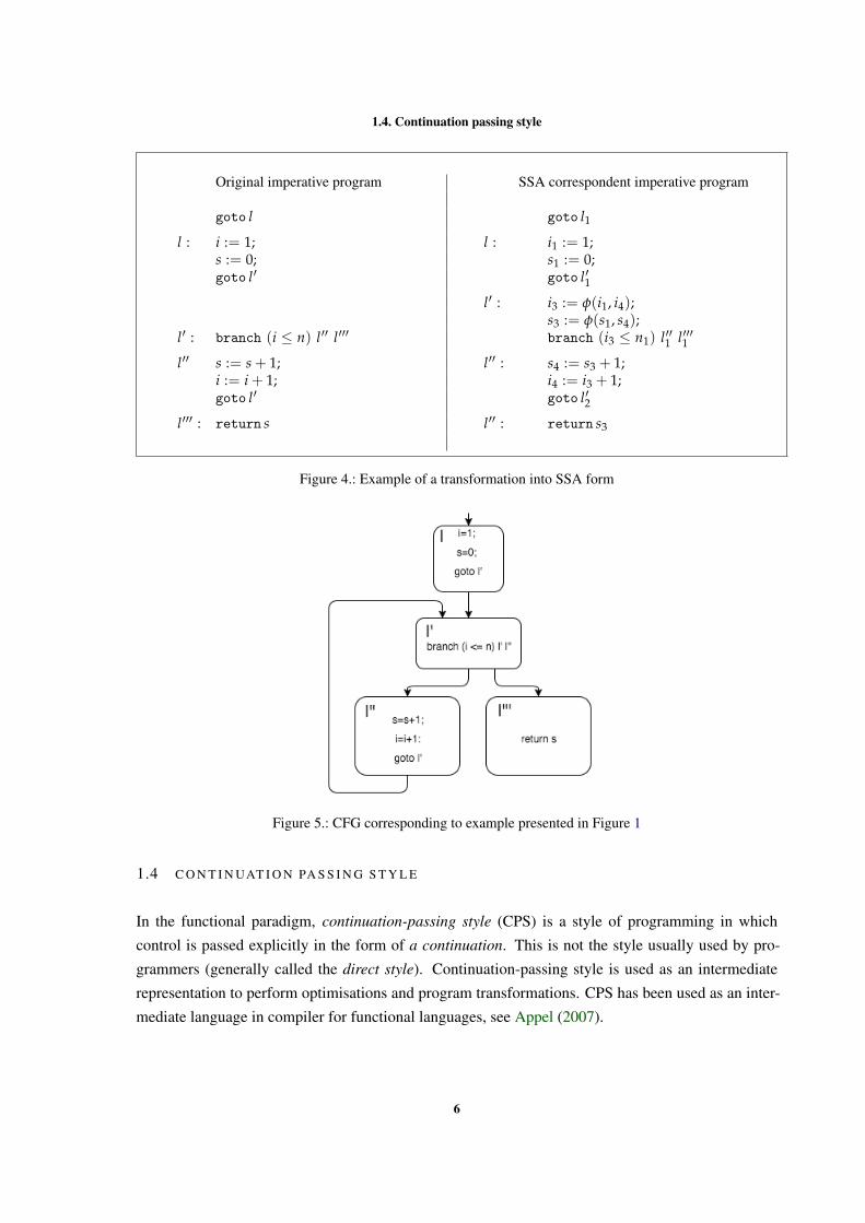
The apparent simplicity of the SSA conversion of the code snippet example given above is mis-

leading. For program with control flow commands (for instance, if and while or goto commands)

the translation to SSA form cannot be done solely by tagging variables: to handle it one must insert

the so-called φ-functions, which control the merging of data flow edges entering code blocks. For

instance, where two control-flow edges join together, carrying different values of some variable, one

must somehow merge the two values. This is done with the help of a φ-function, which is a notational

trick. In some node with two in-edges, the expression φ(a, b) has the value a if one reaches this node

on the first in-edge, and b if one comes in on the second in-edge. The semantics of φ-functions is in

the seminal paper by Cytron et al. (1991):

”If control reaches node j from its kth predecessor, then the run-time support remembers

k while executing the φ-functions in j. The value of φ(x1, x2, ...) is just the value of the

kth operand. Each execution of a φ-function uses only one of the operands, but which

one depends on the flow of control just before entering j.”

Let us illustrate the translation to SSA form with an example in Figure 4.

There may be several SSA forms for a single control-flow graph program. As the number of φ-

functions directly impacts size of the SSA form and the quality of the subsequent optimisations it

is important that SSA generators for real compilers produce a SSA form with a minimal number of

φ-functions. Implementations of minimal SSA generally rely on the notion of dominance frontier to

choose where to insert φ-functions, as indicated, for instance, in (Cytron et al., 1991).

The Control Flow Graph (CFG) is a representation, using graph notation, of all paths that might be

traversed a program during execution. In a CFG, node A dominates node B if any path from the start

to node B must go though A. There is a vast body of work on efficient methods of computing min-

imal SSA form and SSA-based optimisations. General references are Appel (1998b) and Muchnick

(1997a).

5

1.4. Continuation passing style

Original imperative program SSA correspondent imperative program

goto l goto l1

l : i := 1; l : i1 := 1;s := 0; s1 := 0;goto l′ goto l′1

l′ : i3 := φ(i1, i4);s3 := φ(s1, s4);

l′ : branch (i ≤ n) l′′ l′′′ branch (i3 ≤ n1) l′′1 l′′′1

l′′ s := s + 1; l′′ : s4 := s3 + 1;i := i + 1; i4 := i3 + 1;goto l′ goto l′2

l′′′ : return s l′′ : return s3

Figure 4.: Example of a transformation into SSA form

Figure 5.: CFG corresponding to example presented in Figure 1

1.4 C O N T I N UAT I O N PA S S I N G S T Y L E

In the functional paradigm, continuation-passing style (CPS) is a style of programming in which

control is passed explicitly in the form of a continuation. This is not the style usually used by pro-

grammers (generally called the direct style). Continuation-passing style is used as an intermediate

representation to perform optimisations and program transformations. CPS has been used as an inter-

mediate language in compiler for functional languages, see Appel (2007).

6

1.5. Contributions and document structure

A function written in CPS takes an extra argument, the continuation function, which is a function of

one argument. When the CPS function comes to a result value, it returns it by calling the continuation

function with this value as the argument. The continuation represents what should be done with the

result of the function being calculated. This feature, along with some other restrictions on the form

of expressions, makes a number of things explicit (such as function returns, intermediate values, the

order of argument evaluation and tail calls) which are implicit in direct style. λ-calculus in CPS, as

an intermediate representation, is used to expose the semantics of programs, making them easier to

analyze and the optimization process more efficient for functional-language compilers.

It is well known that the SSA form is closely related to λ-terms . (Kelsey, 1995) pointed to a

correspondence between programs in SSA form and λ-terms in CPS. In CPS there is exactly one

binding form for every variable and variable uses are lexically scoped. In SSA there is exactly one

assignment statement for every variable and that statement dominates all uses of the variable.

In Kelsey (1995), Kelsey define syntactic transformation that convert CPS programs into SSA and

vice-versa. Some CPS programs cannot be converted to SSA but these are not pro duced by the usual

CPS transformation. The transformations from CPS into SSA is especially helpful for compiling func-

tional programs. Many optimizations that normally require flow analysis can be performed directly

on functional CPS programs by viewing them as SSA programs.

1.5 C O N T R I B U T I O N S A N D D O C U M E N T S T RU C T U R E

In this work we study the central ideas of static single assignment programs in a context of a simple

imperative language including jump instructions. The fundamental contribution of this thesis is the

proof of correctness of a translation from programs of the base imperative language into the SSA

format. In particular,

• we defined small-step operational semantics for the base imperative language and for the corre-

sponding SSA language;

• we defined a translation from programs of the base language into SSA-programs, and proto-

typed it in Haskell in https://goo.gl/PtfqGJ;

• we developed alternative operational semantics, both for the base imperative language and for

the SSA language, which split the computation, according to whether it involves a jump or not,

and keeps track of information about the variables in order to identify the adequate version of

each variable, when relating execution of a base program and of its SSA translation;

• we proved each of these alternative semantics equivalent to the corresponding small-step se-

mantics;

7

1.5. Contributions and document structure

• we proved soundness and completeness results for the translation, relatively to the alternative

operational semantics, and from these results we proved correctness of the translation relatively

to the initial small-step semantics.

The thesis is organized as follows: In Chapter 2 we formally introduce the syntax and the semantics

of the base imperative language and the SSA language that are used in this work. In Chapter 3 we

present in every detail a function that translates from base imperative programs into SSA-programs.

Chapter 4 is entirely devoted to the proof of correctness of the translation defined. In Chapter 5 we

discuss some possible improvements to the translation function and the relation of SSA-programs and

the functional programming paradigm. Finally we draw some conclusions and directions for future

work.

8

2

I M P E R AT I V E L A N G UAG E A N D S I N G L E A S S I G N M E N T F O R M

In this chapter we introduce a base imperative language and a SSA language that will be used in our

study. For the sake of simplicity we will refer to SSA format just as SA form. We will call GL (short

for Goto Language) to the imperative language. Let us begin by introducing some general notation

used for functions and lists.

N OTAT I O N : Given a function f , dom ( f ) denotes the domain of f and f [x 7→ a] denotes the

function that maps x to a and any other value y to f (y). We also use the notation [x 7→ g(x)| x ∈A] to represent the function with domain A generated by g. For a set B ⊆ dom ( f ), f (B) =

{ f (x) | x ∈ B}.For every A, we let A∗ denote the set of lists of elements of A, and [ ] denote the empty list. ~a ranges

over A+, if a ranges over A. #~a denotes the length of~a. ~a[n] with n≤#~a denotes the nth element of~a.

For convenience, we will sometimes write non-empty lists in the form h : t, where h denotes the first

element of the list (its head) and t the rest of it (its tail).

We use the ++ infix operator for the concatenation of two lists.

Given a total function f : X → Y and a partial function g : X ⇀ Y, we define f ⊕ g : X → Y as

follows:

( f ⊕ g)(x) =

{g(x) if x ∈ dom (g)f (x) if x 6∈ dom (g)

i.e., g overrides f but leaves f unchanged at points where g is not defined.

2.1 T H E G OT O L A N G UAG E GL

GL is a simple “goto” language whose programs are defined as sequences of labeled blocks with an

entry point. Blocks are sequences of assignments that end with a jump or a return instruction, if the

program ends in the block. Labels are used as names for the blocks.

9

2.1. The Goto Language GL

2.1.1 Syntax

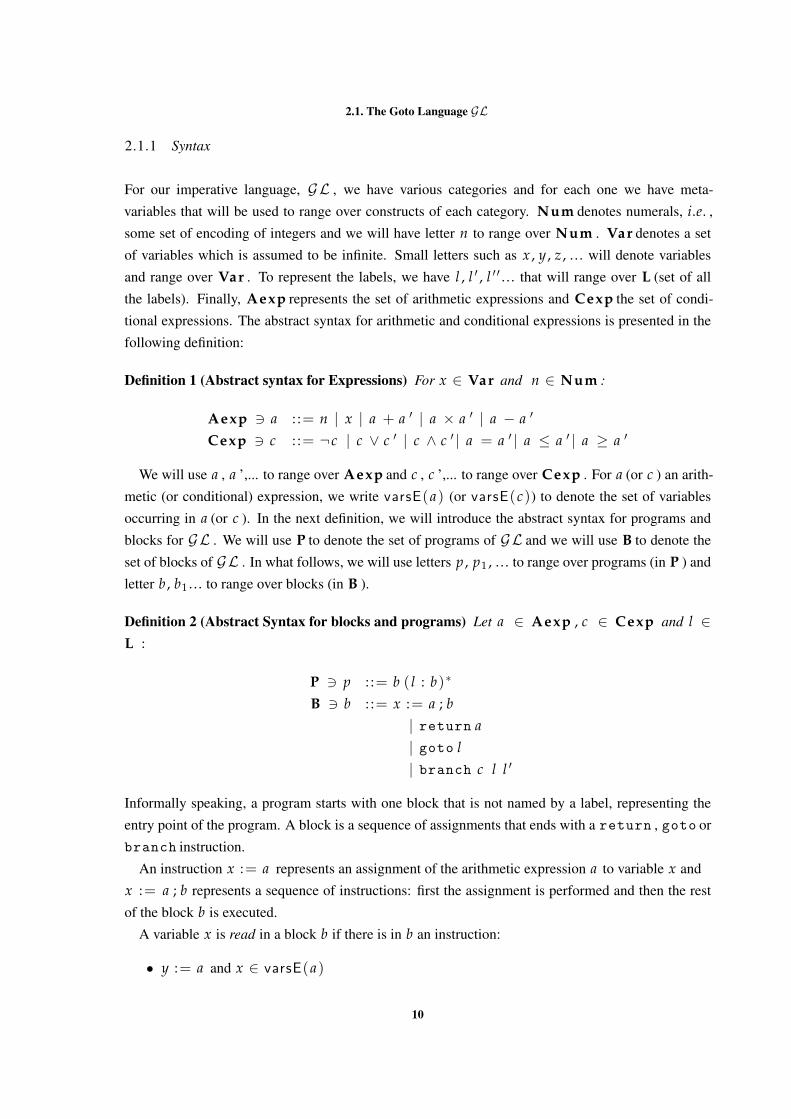
For our imperative language, GL , we have various categories and for each one we have meta-

variables that will be used to range over constructs of each category. Num denotes numerals, i.e. ,

some set of encoding of integers and we will have letter n to range over Num . Var denotes a set

of variables which is assumed to be infinite. Small letters such as x , y , z , . . . will denote variables

and range over Var . To represent the labels, we have l , l ′ , l ′ ′ . . . that will range over L (set of all

the labels). Finally, Aexp represents the set of arithmetic expressions and Cexp the set of condi-

tional expressions. The abstract syntax for arithmetic and conditional expressions is presented in the

following definition:

Definition 1 (Abstract syntax for Expressions) For x ∈ Var and n ∈ Num :

Aexp 3 a : := n | x | a + a ′ | a × a ′ | a − a ′

Cexp 3 c : := ¬c | c ∨ c ′ | c ∧ c ′ | a = a ′ | a ≤ a ′ | a ≥ a ′

We will use a , a ’,... to range over Aexp and c , c ’,... to range over Cexp . For a (or c ) an arith-

metic (or conditional) expression, we write varsE(a) (or varsE(c)) to denote the set of variables

occurring in a (or c ). In the next definition, we will introduce the abstract syntax for programs and

blocks for GL . We will use P to denote the set of programs of GL and we will use B to denote the

set of blocks of GL . In what follows, we will use letters p , p1 , . . . to range over programs (in P ) and

letter b , b1 . . . to range over blocks (in B ).

Definition 2 (Abstract Syntax for blocks and programs) Let a ∈ Aexp , c ∈ Cexp and l ∈L :

P 3 p : := b ( l : b)∗

B 3 b : := x := a ; b| return a| goto l| branch c l l ′

Informally speaking, a program starts with one block that is not named by a label, representing the

entry point of the program. A block is a sequence of assignments that ends with a return , goto or

branch instruction.

An instruction x := a represents an assignment of the arithmetic expression a to variable x and

x := a ; b represents a sequence of instructions: first the assignment is performed and then the rest

of the block b is executed.

A variable x is read in a block b if there is in b an instruction:

• y := a and x ∈ varsE(a)

10

2.1. The Goto Language GL

• return a and x ∈ varsE(a)

• branch c l l ′ and x ∈ varsE(c)

We say that a variable is used in a block b if is read or assigned in that block. The blocks, B , are a

sequences of assignments that end with a jump instruction in which:

• goto l represents a jump from the current block to the block labeled l;

• branch c l l′ represents a conditional jump, which means it only jumps to the block labeled lif c is evaluated to true , otherwise it jumps to the block labeled l′;

• return a instruction finishes execution and returns expression a as “result”.

We say that a label is defined in a program p when it is the identifier/name for some block b. We

write (l : b) ∈ p to denote that in program p there is a block b labeled with l. We say that a label is

invoked by an instruction in a program p, if there is a goto or branch instruction that uses the label

as argument, i.e. , we say that l is invoked in a block b if b contains an instruction branch c l l′ ,branch c l′ l or goto l . We say that l is invoked in a program p, if it is invoked in a block of p.

We will be interested only in a subset of P , well formed programs that we define now.

Definition 3 (Well-formed program) Let p ∈ P . We say that p is well-formed, denoted wfProg(p) ,

if:

1. each label is defined at most once;

2. each label invoked in an instruction of p, is defined in p.

Note that, for a well-formed program p, if a label l is defined we use (l : b) ∈ p to identify the

block b associated to l.A control flow graph (CFG) is a graphical representation, of all paths that might be traversed

through a program during its execution. Let us give a small example of a well formed program.

11

2.1. The Goto Language GL

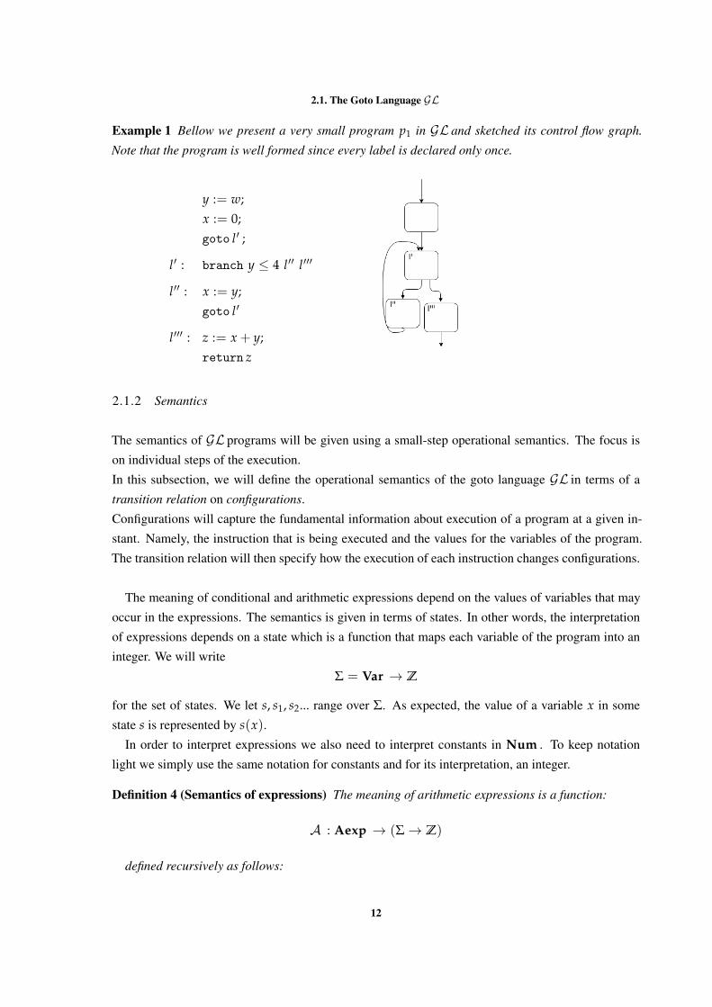
Example 1 Bellow we present a very small program p1 in GL and sketched its control flow graph.

Note that the program is well formed since every label is declared only once.

y := w;x := 0;goto l′ ;

l′ : branch y ≤ 4 l′′ l′′′

l′′ : x := y;goto l′

l′′′ : z := x + y;return z

2.1.2 Semantics

The semantics of GL programs will be given using a small-step operational semantics. The focus is

on individual steps of the execution.

In this subsection, we will define the operational semantics of the goto language GL in terms of a

transition relation on configurations.

Configurations will capture the fundamental information about execution of a program at a given in-

stant. Namely, the instruction that is being executed and the values for the variables of the program.

The transition relation will then specify how the execution of each instruction changes configurations.

The meaning of conditional and arithmetic expressions depend on the values of variables that may

occur in the expressions. The semantics is given in terms of states. In other words, the interpretation

of expressions depends on a state which is a function that maps each variable of the program into an

integer. We will write

Σ = Var → Z

for the set of states. We let s, s1, s2... range over Σ. As expected, the value of a variable x in some

state s is represented by s(x).In order to interpret expressions we also need to interpret constants in Num . To keep notation

light we simply use the same notation for constants and for its interpretation, an integer.

Definition 4 (Semantics of expressions) The meaning of arithmetic expressions is a function:

A : Aexp → (Σ→ Z)

defined recursively as follows:

12

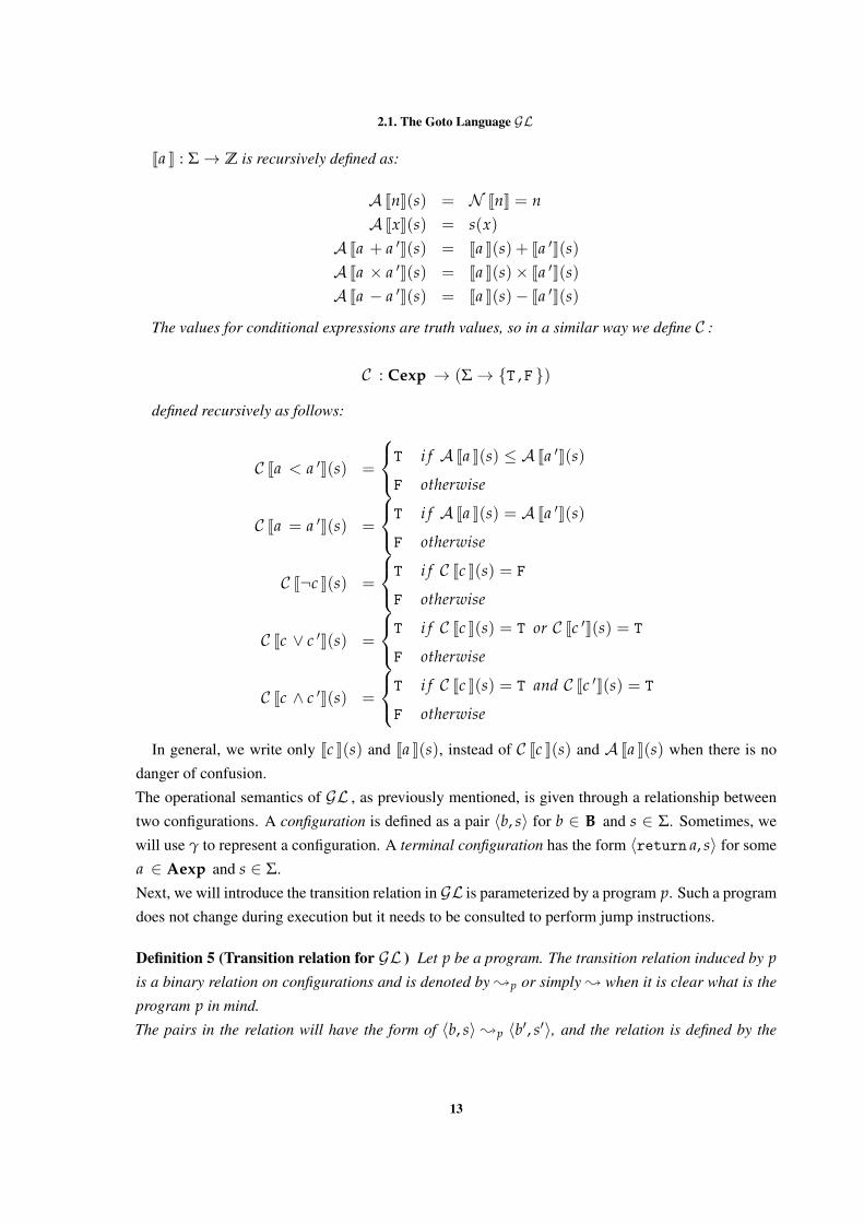
2.1. The Goto Language GL

Ja K : Σ→ Z is recursively defined as:

A JnK(s) = N JnK = nA JxK(s) = s(x)

A Ja + a ′K(s) = Ja K(s) + Ja ′K(s)A Ja × a ′K(s) = Ja K(s)× Ja ′K(s)A Ja − a ′K(s) = Ja K(s)− Ja ′K(s)

The values for conditional expressions are truth values, so in a similar way we define C :

C : Cexp → (Σ→ {T , F })

defined recursively as follows:

C Ja < a ′K(s) =

T i f A Ja K(s) ≤ A Ja ′K(s)

F otherwise

C Ja = a ′K(s) =

T i f A Ja K(s) = A Ja ′K(s)

F otherwise

C J¬c K(s) =

T i f C Jc K(s) = F

F otherwise

C Jc ∨ c ′K(s) =

T i f C Jc K(s) = T or C Jc ′K(s) = T

F otherwise

C Jc ∧ c ′K(s) =

T i f C Jc K(s) = T and C Jc ′K(s) = T

F otherwise

In general, we write only Jc K(s) and Ja K(s), instead of C Jc K(s) and A Ja K(s) when there is no

danger of confusion.

The operational semantics of GL , as previously mentioned, is given through a relationship between

two configurations. A configuration is defined as a pair 〈b, s〉 for b ∈ B and s ∈ Σ. Sometimes, we

will use γ to represent a configuration. A terminal configuration has the form 〈return a, s〉 for some

a ∈ Aexp and s ∈ Σ.

Next, we will introduce the transition relation in GL is parameterized by a program p. Such a program

does not change during execution but it needs to be consulted to perform jump instructions.

Definition 5 (Transition relation for GL ) Let p be a program. The transition relation induced by pis a binary relation on configurations and is denoted by ;p or simply ; when it is clear what is the

program p in mind.

The pairs in the relation will have the form of 〈b, s〉;p 〈b′, s′〉, and the relation is defined by the

13

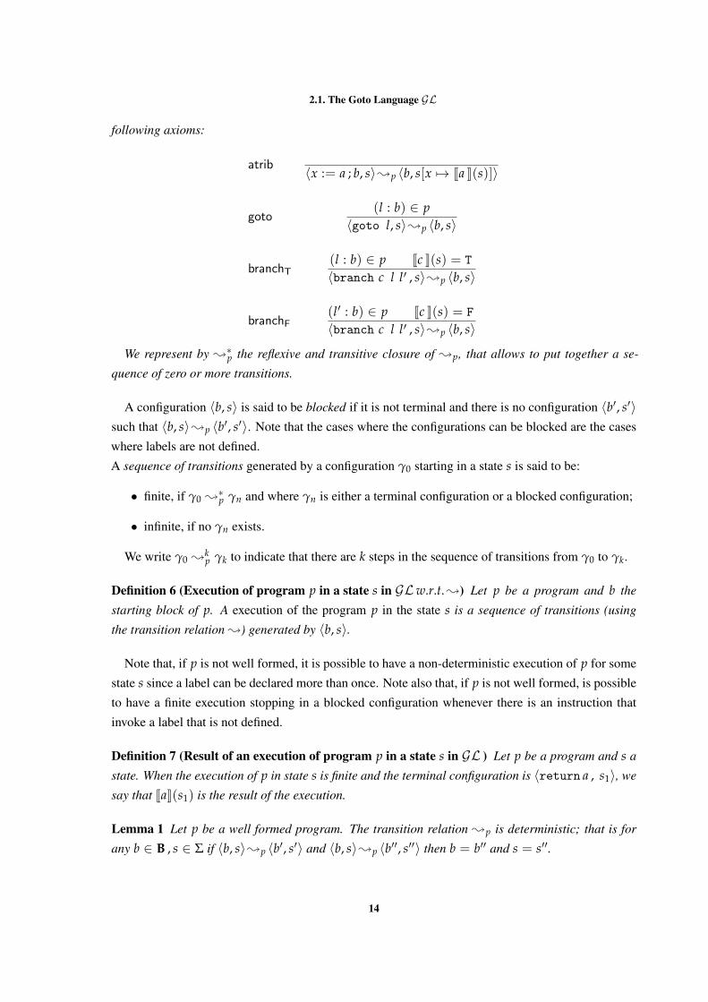
2.1. The Goto Language GL

following axioms:

atrib 〈x := a ; b, s〉;p 〈b, s[x 7→ Ja K(s)]〉

goto(l : b) ∈ p

〈goto l, s〉;p 〈b, s〉

branchT(l : b) ∈ p Jc K(s) = T

〈branch c l l′ , s〉;p 〈b, s〉

branchF(l′ : b) ∈ p Jc K(s) = F

〈branch c l l′ , s〉;p 〈b, s〉

We represent by ;∗p the reflexive and transitive closure of ;p, that allows to put together a se-

quence of zero or more transitions.

A configuration 〈b, s〉 is said to be blocked if it is not terminal and there is no configuration 〈b′, s′〉such that 〈b, s〉;p 〈b′, s′〉. Note that the cases where the configurations can be blocked are the cases

where labels are not defined.

A sequence of transitions generated by a configuration γ0 starting in a state s is said to be:

• finite, if γ0 ;∗p γn and where γn is either a terminal configuration or a blocked configuration;

• infinite, if no γn exists.

We write γ0 ;kp γk to indicate that there are k steps in the sequence of transitions from γ0 to γk.

Definition 6 (Execution of program p in a state s in GLw.r.t.;) Let p be a program and b the

starting block of p. A execution of the program p in the state s is a sequence of transitions (using

the transition relation ;) generated by 〈b, s〉.

Note that, if p is not well formed, it is possible to have a non-deterministic execution of p for some

state s since a label can be declared more than once. Note also that, if p is not well formed, is possible

to have a finite execution stopping in a blocked configuration whenever there is an instruction that

invoke a label that is not defined.

Definition 7 (Result of an execution of program p in a state s in GL ) Let p be a program and s a

state. When the execution of p in state s is finite and the terminal configuration is 〈return a , s1〉, we

say that JaK(s1) is the result of the execution.

Lemma 1 Let p be a well formed program. The transition relation ;p is deterministic; that is for

any b ∈ B , s ∈ Σ if 〈b, s〉;p 〈b′, s′〉 and 〈b, s〉;p 〈b′′, s′′〉 then b = b′′ and s = s′′.

14

2.2. SA language

Proof. If follows from item 1 of Definition 3 and with induction on the derivation. 2

Proposition 1 Let p be a well-formed program.

(i) The execution of program p in state s is deterministic: given a state s ∈ Σ, exists exactly one

sequence of transitions generated by 〈b, s〉 where b is the starting block of program p;

(ii) The execution of program p in state is finite: if it ends, it ends in a terminal configuration.

Proof. It follows directly from Lemma 1. Also, it is a direct consequence of item 2 of Definition 3.

2

Example 2 The execution of the program p1 of Example 1 with a initial state s0 such that s0(w) = 5is:

〈y := 5; x := 0; goto l′ , s0〉;p1 〈x := 0; goto l′ , s1〉;p1 〈goto l′ , s2〉;p1

〈branch y ≤ 4 l′′ l′′′ , s2 〉;p1 〈z := x + y; return z , s2〉;p1 〈return z , s3〉where: s1 = s0[y 7→ 5], s2 = s1[x 7→ 0] and s3 = s2[z 7→ 5]In this example, the result of the execution is 5.

Example 3 The execution of the program p1 of Example 1) with a initial state s0 such that s0(w) = 3is:

〈y := 3; x := 0; goto l′ , s0〉;p1 〈x := 0; goto l′ , s1〉;p1 〈goto l′ , s2〉;p1

〈branch y ≤ 4 l′′ l′′′ , s2 〉;p1 〈x := y; goto l′ , s2〉;p1 〈branch y ≤ 4 l′′ l′′′ , s2 〉;p1 〈x :=y; goto l′ , s2〉;p1 (...)

where: s1 = s0[y 7→ 3] and s2 = s1[x 7→ 0].Therefore, the program loops.

2.2 S A L A N G UAG E

We will now present a variant of the programs in P that are in SSA form. For the sake of simplicity,

we will call those single assignment (SA) programs and represent them by PSA . The basic idea in

the SA programs is to create versions of variables so that a version of a variable does not get assigned

more than once in a SA block.

2.2.1 Syntax

In this subsection, we present a variant of the GLwhere the program is in single assignment form.

Syntactically, relatively to the GL , there are essentially three differences:

15

2.2. SA language

1. Variables now come with an index over N. We let a VarSA = Var ×N be the set of SA

variables and we will write xi to denote (x, i) ∈ VarSA ;

2. Similarly, labels come with an index over N. We let a LSA = L ×N be the set of SA labels

and we will write li to denote (l, i) ∈ LSA ;

3. There is a new ingredient that, as usually in the literature, we call φ-functions, which syntacti-

cally we write as φ(~xj) where ~xj is a vector of SA variables, and semantically will be responsible

to control what is the correct version of a variable to use at a given point of program execution.

More specifically, the φ-functions let us decide which version of the variable should we use

by knowing from which block came the edge. The k’th argument of φ(~xj) will be used when

control reach the block from goto lk . In the rest of the document, instead of using the word edge

we will normally use the word door, so goto lk can be read as: execute the block l knowing we

arrive at it through door k.

The synchronization of variables will happen at the beginning of the blocks. An SA block will

start with a list of assignments of φ-functions, which we generally represent by φ and let Φdenote the set of lists of arguments of φ-functions. We denote by dom (φ) the set of variables

assigned in φ. For instance, dom (x1 := φ(x5, x3), y2 := φ(y1, y4)) = {x1, y2}.

The specification of SA Programs is captured by the abstract syntax:

Definition 8 (Abstract syntax for SA programs)

Φ 3 φ ::= (xi := φ(~xj))∗

PSA 3 p′ ::= b(l : φb)∗

BSA 3 b′ ::= xi := a ; b| return a| goto li| branch c li l′j

We will use p′, p′′, ... to represent SA programs (in PSA ) and b′, b′′.. to represent SA blocks (in BSA ).

Recall that p, p1, ... are used for programs in P .

Example 4 Example of program p′1 - SA version of program p1 presented in Example 1:

16

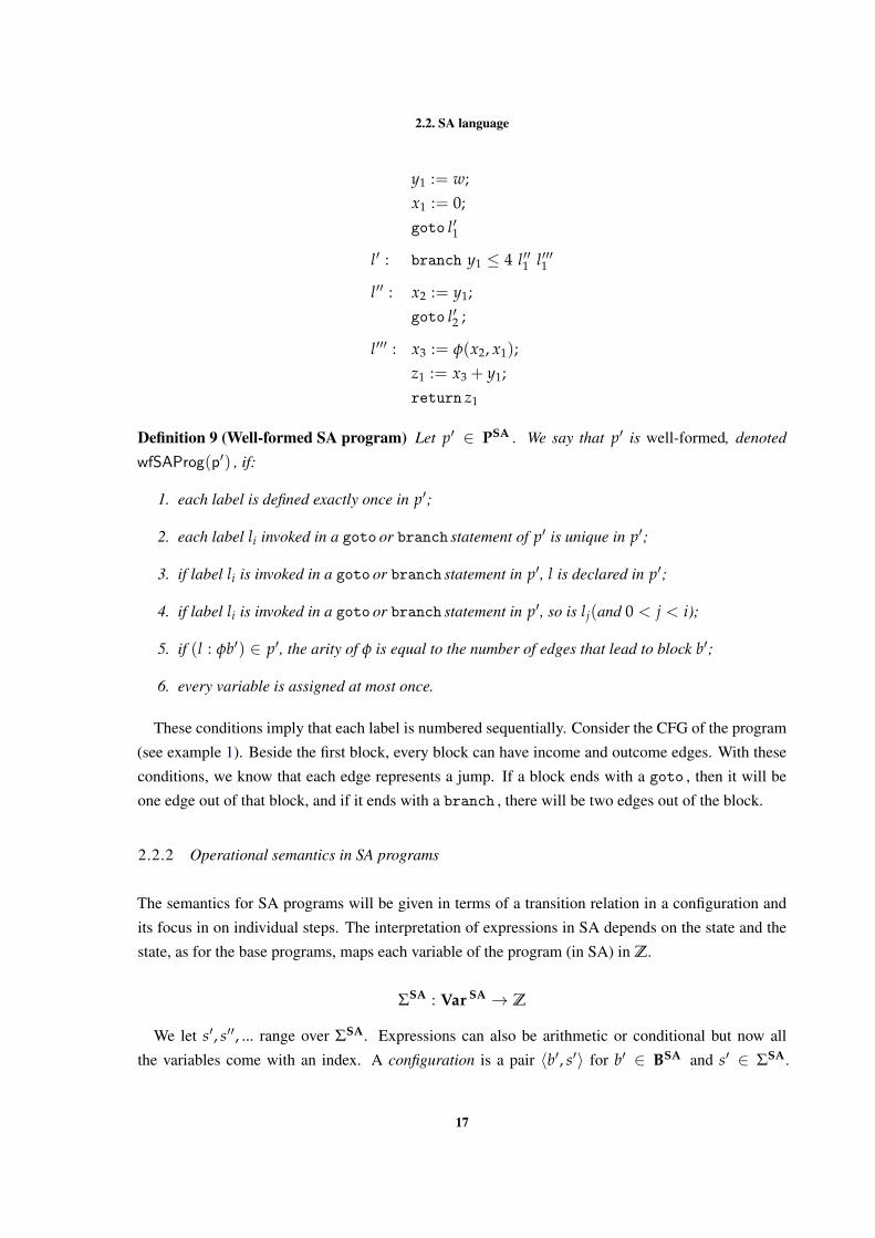
2.2. SA language

y1 := w;x1 := 0;goto l′1

l′ : branch y1 ≤ 4 l′′1 l′′′1

l′′ : x2 := y1;goto l′2 ;

l′′′ : x3 := φ(x2, x1);z1 := x3 + y1;return z1

Definition 9 (Well-formed SA program) Let p′ ∈ PSA . We say that p′ is well-formed, denoted

wfSAProg(p′) , if:

1. each label is defined exactly once in p′;

2. each label li invoked in a goto or branch statement of p′ is unique in p′;

3. if label li is invoked in a goto or branch statement in p′, l is declared in p′;

4. if label li is invoked in a goto or branch statement in p′, so is lj(and 0 < j < i);

5. if (l : φb′) ∈ p′, the arity of φ is equal to the number of edges that lead to block b′;

6. every variable is assigned at most once.

These conditions imply that each label is numbered sequentially. Consider the CFG of the program

(see example 1). Beside the first block, every block can have income and outcome edges. With these

conditions, we know that each edge represents a jump. If a block ends with a goto , then it will be

one edge out of that block, and if it ends with a branch , there will be two edges out of the block.

2.2.2 Operational semantics in SA programs

The semantics for SA programs will be given in terms of a transition relation in a configuration and

its focus in on individual steps. The interpretation of expressions in SA depends on the state and the

state, as for the base programs, maps each variable of the program (in SA) in Z.

ΣSA : Var SA → Z

We let s′, s′′, ... range over ΣSA. Expressions can also be arithmetic or conditional but now all

the variables come with an index. A configuration is a pair 〈b′, s′〉 for b′ ∈ BSA and s′ ∈ ΣSA.

17

2.2. SA language

A terminal configuration has the same form of a terminal configuration in GL : 〈return a , s′〉 for

s ∈ ΣSA and a ∈ Aexp . For the constants in Num , we will use the same notation: an integer.

Next, we will introduce the transition relation in SA Programs parameterized by a SA program p′.This relation is analogous to the transition relation in GL for a program p. The difference is in the

way of denoting the variables, which now have an index.

Definition 10 (Operational semantics to SA programs) Let p′ be a well formed program in SA. The

transition relation induced by p′ is binary and is represented by ;p′ . The pairs have the form by

〈b′, s′〉;p′ 〈b′′, s′′〉. This transition relation is defined by the following axioms:

atrib 〈xi := a ; b, s〉;p′ 〈b, s[xi 7→ Ja K(s)]〉

goto(l : φ b′) ∈ p′

〈goto li, s〉;p′ 〈b, upd (φ, i, s))〉

branchT(l : φ b′) ∈ p′ Jc K(s) = true

〈branch c li l′j , s〉;p′ 〈b, upd (φ, i, s))〉

branchF(l : φ b′) ∈ p′ Jc K(s) = false

〈branch c li l′j , s〉;p′ 〈b, upd (φ, j, s))〉

where upd is the update function defined as follows:

upd : Φ×N× ΣSA → ΣSA

(φ, n, s) 7−→ s[x 7→ J~x[n]K(s)|x := φ(~x) ∈ φ]

The upd function select the right version of the variable in the beginning of each block. Note that,

because p′ ∈ PSA is well-formed, the upd function is well-defined (item 5 of Definition 9).

Lemma 2 Let p′ be a well formed program. The transition relation ;p′ is deterministic; that is for

any b′ ∈ BSA , s′ ∈ ΣSA if 〈b′, s′〉;p 〈b′′, s′′〉 and 〈b′, s′〉;p 〈b′′′, s′′′〉 then b′′ = b′′′ and s′′ = s′′′.

Proof. If follows directly from Item 1, 2 and 3 of Definition 9. 2

Definition 11 (Execution of program p′ in a state s′ in SA w.r.t.;) Let p′ be a SA program and b′

the starting block of p′. A execution of the program p′ in the state s′ is a sequence of transitions using

the transition relation ; generated by 〈b′, s′〉.

Note that, if p′ is not well formed, it is possible to have a variable assigned more than once, and it

is possible to have variables that were not in the φ domain. Moreover, it is possible to have a jump

instruction in p′ that leads to no block, since it is possible to invoke a label that is not defined. Similarly

to programs in GL , if p′ is not well formed it is possible to have a non-deterministic execution of p′

for some state s′ since a label can be declared more than once.

18

2.2. SA language

Definition 12 (Result of an execution of program p in a state s in SA) Let p′ be a program in SA

and s′ a state. When the execution of p′ in state s′ is finite and the terminal configuration is 〈return a′ , s′1〉,we say that Ja′K(s′1) is the result of the execution.

Proposition 2 Let p′ be a well-formed SA program.

(i) The execution of program p′ in state s′ is deterministic: given a state s′ ∈ ΣSA, exists exactly

one sequence of transitions generated by 〈b′, s′〉 were b’ is the starting point of p′;

(ii) If the execution of program p′ in state s′ is finite, then it ends in a terminal configuration.

Proof. It follows directly from Lemma 2. 2

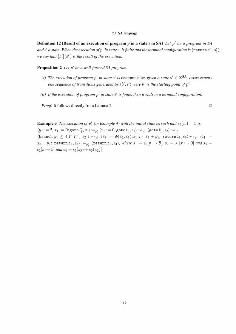
Example 5 The execution of p′1 (in Example 4) with the initial state s0 such that s0(w) = 5 is:

〈y1 := 5; x1 := 0; goto l′1 , s0〉;p′1〈x1 := 0; goto l′1 , s1〉;p′1

〈goto l′1 , s2〉;p′1〈branch y1 ≤ 4 l′′1 l′′′1 , s2 〉 ;p′1

〈x3 := φ(x2, x1); z1 := x3 + y1; return z1 , s3〉 ;p′1〈z1 :=

x3 + y1; return z1 , s3〉 ;p′1〈return z1 , s4〉, where s1 = s0[y 7→ 5], s2 = s1[x 7→ 0] and s3 =

s2[z 7→ 5] and s4 = s3[x3 7→ s3(x2)]

19

3

A T R A N S L AT I O N I N T O S A F O R M

In this chapter we present an algorithm to transform GL programs into SA format. The algorithm

has been implemented in Haskell (the code is in Appendix A). We will prove the correctness of the

translation in the next chapter.

Throughout this chapter we assume that the programs in P are always well formed.

3.1 T R A N S L AT I N G I N T O S A F O R M

A program in P has an entrance block (with no label associated) and a sequence of labeled blocks.

In order to uniform the translation algorithm, we will introduce a distinguished label, denoted by •,that we will associate to the entrance block. Of course the special label • can not be invoked in the

program.

The programs we translate belong to the class P• defined by:

P• 3 p ::= (• : b)(l : b)∗

The SA programs produced by the translation will belong to the class PSA• defined by:

PSA• 3 p′ ::= (• : b′)(l : φb′)∗

The conversion of a program from P to P• and from PSA• to PSA is trivial (just add/remove the

label •) and deserve no further comments. We let L• represent the set of labels enriched with the

distinguished label •, i.e. , L• = L ∪ {•}. Programs in P• can be seen as elements of (L• × B )∗.

The translation from P• into PSA• is performed by function T and is done in two steps. In the first

step we create an intermediate structure composed by a quasi SA program (SA program without φ-

functions) - PI• = (L• × BSA )∗ - and a context that registers information of the translation process.

The second step uses this intermediate structure to add the φ-functions to the quasi SA program,

producing a program in PSA• .The translation process is illustrated in Figure 6. We name the first step

R (after renaming) and the second step S (after synchronization).

TheR function does three different tasks:

20

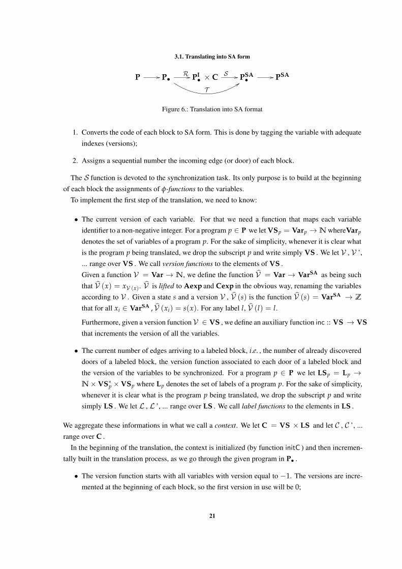
3.1. Translating into SA form

P // P•R //

T99

PI• × C S // PSA

• // PSA

Figure 6.: Translation into SA format

1. Converts the code of each block to SA form. This is done by tagging the variable with adequate

indexes (versions);

2. Assigns a sequential number the incoming edge (or door) of each block.

The S function is devoted to the synchronization task. Its only purpose is to build at the beginning

of each block the assignments of φ-functions to the variables.

To implement the first step of the translation, we need to know:

• The current version of each variable. For that we need a function that maps each variable

identifier to a non-negative integer. For a program p ∈ P we let VSp = Varp →N whereVarp

denotes the set of variables of a program p. For the sake of simplicity, whenever it is clear what

is the program p being translated, we drop the subscript p and write simply VS . We let V , V ’,

... range over VS . We call version functions to the elements of VS .

Given a function V = Var → N, we define the function V = Var → VarSA as being such

that V (x) = xV (x). V is lifted to Aexp and Cexp in the obvious way, renaming the variables

according to V . Given a state s and a version V , V (s) is the function V (s) = VarSA → Z

that for all xi ∈ VarSA , V (xi) = s(x). For any label l, V (l) = l.

Furthermore, given a version function V ∈ VS , we define an auxiliary function inc :: VS → VSthat increments the version of all the variables.

• The current number of edges arriving to a labeled block, i.e. , the number of already discovered

doors of a labeled block, the version function associated to each door of a labeled block and

the version of the variables to be synchronized. For a program p ∈ P we let LSp = Lp →N×VS∗p ×VSp where Lp denotes the set of labels of a program p. For the sake of simplicity,

whenever it is clear what is the program p being translated, we drop the subscript p and write

simply LS . We let L , L ’, ... range over LS . We call label functions to the elements in LS .

We aggregate these informations in what we call a context. We let C = VS × LS and let C , C ’, ...

range over C .

In the beginning of the translation, the context is initialized (by function initC ) and then incremen-

tally built in the translation process, as we go through the given program in P• .

• The version function starts with all variables with version equal to −1. The versions are incre-

mented at the beginning of each block, so the first version in use will be 0;

21

3.1. Translating into SA form

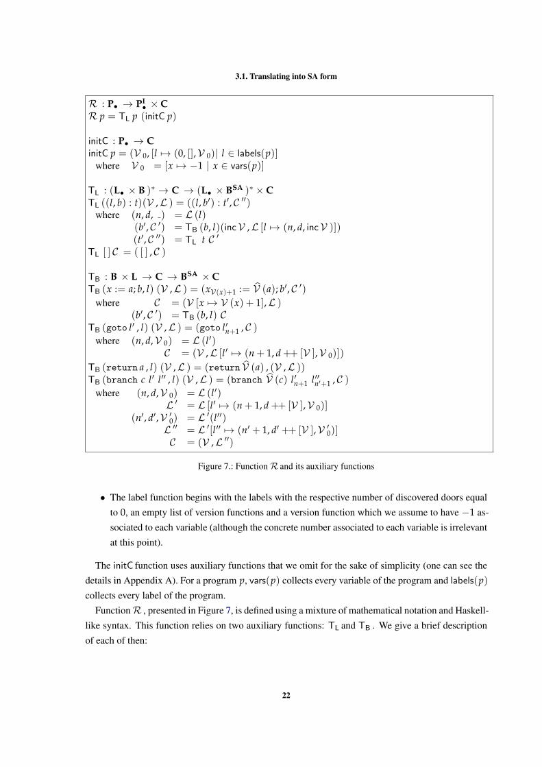
R : P• → PI• × C

R p = TL p (initC p)

initC : P• → CinitC p = (V 0, [l 7→ (0, [],V 0)| l ∈ labels(p)]

where V 0 = [x 7→ −1 | x ∈ vars(p)]

TL : (L• × B )∗ → C → (L• × BSA )∗ × CTL ((l, b) : t)(V ,L ) = ((l, b′) : t′, C ′′)

where (n, d, ) = L (l)(b′, C ′) = TB (b, l)(incV ,L [l 7→ (n, d, incV )])(t′, C ′′) = TL t C ′

TL [ ] C = ( [ ] , C )

TB : B × L → C → BSA × CTB (x := a; b, l) (V ,L ) = (xV(x)+1 := V (a); b′, C ′)

where C = (V [x 7→ V (x) + 1],L )(b′, C ′) = TB (b, l) C

TB (goto l′ , l) (V ,L ) = (goto l′n+1 , C )where (n, d,V 0) = L (l′)

C = (V ,L [l′ 7→ (n + 1, d ++ [V ],V 0)])

TB (return a , l) (V ,L ) = (return V (a) , (V ,L ))TB (branch c l′ l′′ , l) (V ,L ) = (branch V (c) l′n+1 l′′n′+1 , C )

where (n, d,V 0) = L (l′)L ′ = L [l′ 7→ (n + 1, d ++ [V ],V 0)]

(n′, d′,V ′0) = L ′(l′′)L ′′ = L ′[l′′ 7→ (n′ + 1, d′ ++ [V ],V ′0)]C = (V ,L ′′)

Figure 7.: FunctionR and its auxiliary functions

• The label function begins with the labels with the respective number of discovered doors equal

to 0, an empty list of version functions and a version function which we assume to have −1 as-

sociated to each variable (although the concrete number associated to each variable is irrelevant

at this point).

The initC function uses auxiliary functions that we omit for the sake of simplicity (one can see the

details in Appendix A). For a program p, vars(p) collects every variable of the program and labels(p)collects every label of the program.

FunctionR , presented in Figure 7, is defined using a mixture of mathematical notation and Haskell-

like syntax. This function relies on two auxiliary functions: TL and TB . We give a brief description

of each of then:

22

3.1. Translating into SA form

sync :: L → C → Φsync l ( ,L ) = [ xV (x) := φ([xV ′(x) | V ′ ← d]) | x ∈ dom (V ) ]

where ( , d,V ) = L (l)

S :: PI• × C → PSA

•S ([ ], ) = [ ]S ((•, b) : t, C ) = (•, [ ], b) : S (t, C )S ((l, b) : t , C ) = (l , sync l C , b) : S (t, C )

Figure 8.: Functions sync and S

T :: P• → PSA•

T p = S (R p)

Figure 9.: Function T

• TL iterates over the program, translating each block and carrying the corresponding auxiliary

context. It begins by incrementing the version of each variable, in order to spare a version for

synchronization. This task is performed by the auxiliary function inc. The synchronization

version of the block being translated is registered in the label function, by associating it to the

label of the block.

• TB starts the translation of a labeled block. TB receives the block to be translated, its label and

the context. TB is responsible for:

(i) tagging the variables according to the version function and the SA format;

(ii) tagging the labels of the goto and branch commands according to the label function.

Moreover, it updates the context coherently.

After we get the intermediate program (in PI• ), it is necessary to synchronize the variables that can

come from different doors. To do that, we must add the φ-functions. This operation is done by the

function S , which can be seen in Figure 8. For the sake of simplicity, we assume that the φ-functions

sequence follows some predefined order established over the set of variables (any order will do).

The final result of the translation into SA format is obtained by applying firstR and secondly apply

the function S as stated in Figure 6, i.e. , T = S ◦ R . We can see function T in Figure 9.

As it can be seen, this translation function synchronizes every variable of the program at the be-

ginning of each block. This is obviously very inefficient and can be optimized. Using static analysis

techniques it is possible to calculate the optimal placement of φ-functions that leads to a minimum

23

3.1. Translating into SA form

set of φ-functions. We did not follow that path because our focus is to prove the correctness of the

translation with respect to the operational semantics, and we thought it was better to work with a naive

version to begin with. However, we think this translation can be adapted to an optimized version if

previously one calculates the optimal placement of the φ functions. With this information one would

initialize the label function and, in the synchronization phase, the S function would only write the

φ-functions previously calculated. We will say more on this in Chapter 8.

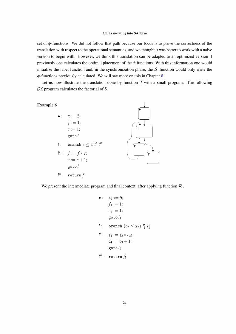
Let us now illustrate the translation done by function T with a small program. The following

GL program calculates the factorial of 5.

Example 6

• : x := 5;f := 1;c := 1;goto l

l : branch c ≤ x l′ l′′

l′ : f := f ∗ c;c := c + 1;goto l

l′′ : return f

We present the intermediate program and final context, after applying functionR .

• : x1 := 5;f1 := 1;c1 := 1;goto l1

l : branch (c2 ≤ x2) l′1 l′′1

l′ : f4 := f3 ∗ c3;c4 := c3 + 1;goto l2

l′′ : return f5

24

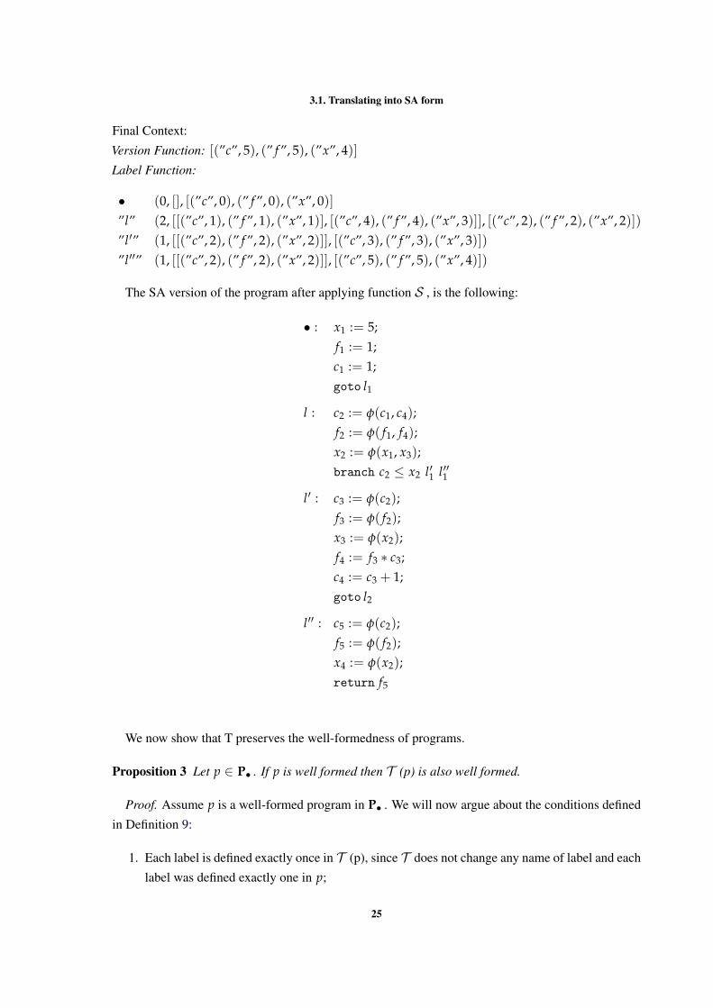
3.1. Translating into SA form

Final Context:

Version Function: [(”c”, 5), (” f ”, 5), (”x”, 4)]Label Function:

• (0, [], [(”c”, 0), (” f ”, 0), (”x”, 0)]”l” (2, [[(”c”, 1), (” f ”, 1), (”x”, 1)], [(”c”, 4), (” f ”, 4), (”x”, 3)]], [(”c”, 2), (” f ”, 2), (”x”, 2)])”l′” (1, [[(”c”, 2), (” f ”, 2), (”x”, 2)]], [(”c”, 3), (” f ”, 3), (”x”, 3)])”l′′” (1, [[(”c”, 2), (” f ”, 2), (”x”, 2)]], [(”c”, 5), (” f ”, 5), (”x”, 4)])

The SA version of the program after applying function S , is the following:

• : x1 := 5;f1 := 1;c1 := 1;goto l1

l : c2 := φ(c1, c4);f2 := φ( f1, f4);x2 := φ(x1, x3);branch c2 ≤ x2 l′1 l′′1

l′ : c3 := φ(c2);f3 := φ( f2);x3 := φ(x2);f4 := f3 ∗ c3;c4 := c3 + 1;goto l2

l′′ : c5 := φ(c2);f5 := φ( f2);x4 := φ(x2);return f5

We now show that T preserves the well-formedness of programs.

Proposition 3 Let p ∈ P• . If p is well formed then T (p) is also well formed.

Proof. Assume p is a well-formed program in P• . We will now argue about the conditions defined

in Definition 9:

1. Each label is defined exactly once in T (p), since T does not change any name of label and each

label was defined exactly one in p;

25

3.1. Translating into SA form

2. The numbering of the doors of each label is done sequentially, so each label li invoked in a

goto or branch statement is unique in T (p);

3. As p is well formed, each label invoked in p is declared so, since T does not change any label

name, T (p) does not have undeclared labels;

4. As stated before, the numbering of the doors of each label is done sequentially, so if a label li is

invoked in a goto or branch statement in T (p), so it is every lj with 0 < j < i;

5. Inspecting the function sync displayed in Figure 8 we can see that the arity of φ-functions is

equal to the number of edges recorded in the label function L , because the sync function is

invoked with the context produced by R after processing all the program. R constructs coher-

ently the context by starting with a context where the number of doors already found for each

label is zero and updating this number each time a label is invoked and recording the version

function associated to the recorded label;

6. By analyzing function TB displayed in Figure 7 one can see that whenever there is an assign-

ment, the variable assigned receives the next index available for that variable and the version

function is updated accordingly. This way, each variable SA will be assigned at most once in

the block;

2

In the next chapter, we will show that function T is correct, that is, that the translated program

preserves the operational semantics of the original program.

26

4

C O R R E C T N E S S O F T H E T R A N S L AT I O N I N T O S A F O R M

In this chapter we prove that the translation of programs in GL to SA form, defined in the previous

chapter, is correct relatively to the defined semantics, that is: the execution of a source program in

GL terminates with a certain result if and only if the execution of its translation into SA terminates

with the same result. This will be established in Corollary 3, as a consequence of soundness and

completeness results from the translation T (Theorem 2 and Theorem 1)

To prove the correctness of the translation function T , we separate each of the transition relations

;p defined in the previous chapter, into two transition relations that will take into account whether

computation continues inside the block or jumps into another block.

In this chapter we will need the auxiliary function that follows. For p ∈ P• , b and b1 ∈ B , x ∈vars(p) and a ∈ Aexp , the notation b =

−−−−→(x := a); b1 will mean that block b comprises a sequence of

assignments−−−−→(x := a), followed by block b1. Also, for V a version function, V [

−−−−→(x := a)] will mean a

new version function V 1 such that:

V 1( [ ] ) = VV 1(x := a;

−−−−−→(y := a1)) = V ′[x 7→ V ′(x) + 1]

whereV ′ = V 1[

−−−−→y := a1]

This corresponds to the evolution of a version function in the process of translating a sequence of

GL -assignments in SA form.

Throughout this chapter we will assume that any p ∈ P• and p′ ∈ PSA• is well-formed.

4.1 S P L I T T I N G T H E T R A N S I T I O N R E L AT I O N O F T H E S O U R C E L A N G UAG E GL

4.1.1 Computation inside block

The new transition relation in GL inside blocks is given through a binary relation on configurations.

The configurations are now triples 〈b , s , V 〉 where b is a block, s is a state and V is a function

that keeps the version of each variable. This will be important in the proofs latter in this chapter,

27

4.1. Splitting the transition relation of the source language GL

since it allows the connection between execution of a program and execution of its translation into

SA form. A terminal configuration inside a block has the form 〈d , s , V 〉 for d = return a , d =

goto l or d = branch c l l ′ , i .e . , a terminal configuration is a configuration that represents

jump or return instructions inside a block.

As this relation represents computation steps inside a block, the only rule that defines the relation has

to do with assignments, as presented in the next definition.

Definition 13 (Transition relation for GL inside blocks) The transition relation inside blocks in GL is

denoted by→ and is the binary relation on configurations given by the following rule:

〈x := a ; b , s , V 〉 → 〈b , s [x 7→ Ja K(s)] , V [x 7→ V (x) + 1 ]〉

We represent by→∗ the reflexive and transitive closure of→, that allows to put together a sequence

of zero or more transitions. By→n we represent n transitions in the relation→.

Lemma 3 Let p ∈ P• . Let b1 , b2 be two blocks. Let s1 , s2 ∈ Σ. Let V 1 , V 2 ∈ VS . We have,

for any n ∈ N0:

〈b1 , s1 , V 1 〉 →n 〈b2 , s2 , V 2 〉 =⇒ 〈b1 , s1 〉;np 〈b2 , s2 〉

Proof. Easy induction on n having in mind Definition 13 and Definition 5 (case atrib). 2

4.1.2 Computation across blocks

We define now the second transition relation to deal with the jump instructions. Here, the configura-

tions are 〈c , s , V 〉 for c := l or c = return a . Next, we present the definition of this relation in

GL . Before this, we will need an auxiliary function, vrs(l ,p), that will produce the correct version

of each variable to be used in the block labeled l in program p, which we define next.

Definition 14 (Synchronized versions) Let p ∈ P• and ( l : b) ∈ p.

vrs( l , p) = [x 7→ i | x i ∈ dom (φ) and ( l : φb ′ ) ∈ T ( p)]

Definition 15 (Transition relation across blocks in GL ) Let p ∈ P• be a program in GL . The

transition relation across blocks induced by p is a binary relation on configurations and is denoted

28

4.1. Splitting the transition relation of the source language GL

by −◦→ p , or simply −◦→, when it is clear the program we have in mind. This transition relation is

defined by the following rules:

return( l : b) ∈ p 〈b , s , V 〉 →∗ 〈return a , s ′ , V ′ 〉

〈 l , s , V 〉 −◦→ p 〈return a , s ′ , V ′ 〉

goto( l : b) ∈ p 〈b , s , V 〉 →∗ 〈goto l ′ , s ′ , V ′ 〉

〈 l , s , V 〉 −◦→ p 〈 l ′ , s ′ , vrs( l ′ , p)〉

branchT( l : b) ∈ p 〈b , s , V 〉 →∗ 〈branch c l ′ l ′ ′ , s ′ , V ′ 〉 Jc K(s ′ ) = T

〈 l , s , V 〉 −◦→ p 〈 l ′ , s ′ , vrs( l ′ , p)〉

branchF( l : b) ∈ p 〈b , s , V 〉 →∗ 〈branch c l ′ l ′ ′ , s ′ , V ′ 〉 Jc K(s ′ ) = F

〈 l , s , V 〉 −◦→ p 〈 l ′ ′ , s ′ , vrs( l ′ ′ , p)〉

In a sequence of transitions across blocks, an intermediate configuration has the form 〈l, s,V 〉 and

a terminal configuration across blocks has the form 〈return a , s′,V ′〉. We represent by −◦→∗p the

reflexive and transitive closure of −◦→p, that allows to put together a sequence of zero or more

transitions. By −◦→np we represent n transitions on −◦→p.

Now we establish some basic results relating the transition relations ; and −◦→ for GL programs.

Lemma 4 Let p ∈ P• and (l : b1) ∈ p. Let s1, s2 ∈ Σ. We have one of the following, for some n:

1. 〈l, s1,V 1〉 −◦→ 〈return a , s2,V 2〉 =⇒ 〈b1, s1〉;n 〈return a , s2〉

2. 〈l, s1,V 1〉 −◦→ 〈l′, s2,V 2〉 implies one of the following rules:

a) 〈b1, s1〉;n 〈goto l′ , s2〉or

b) 〈b1, s1〉;n 〈branch c l′ l′′ , s2〉 and Jc K(s2) = T

or

c) 〈b1, s1〉;n 〈branch c l′′ l′ , s2〉 and Jc K(s2) = F

Proof. Follows easily from Definition 15 and Lemma 3. 2

Lemma 5 Let p ∈ P• and (l : b1), (l′ : b2) ∈ p. Let s1, s2 ∈ Σ. Let n = #−−−−−→(x := e ). We have that:

1. If b1 =−−−−−→(x := e ); return a and 〈b1, s1〉;n 〈return a , s2〉 then, ∀V 1 ∃V 2:

1.1. 〈b1, s1,V 1〉 →n 〈return a , s2,V 2〉

1.2. 〈l, s1,V 1〉 −◦→ 〈return a , s2,V 2〉

2. If b1 =−−−−−→(x := e ); goto l′ and 〈b1, s1〉;n 〈goto l′ , s2〉 then, ∀V 1 ∃V 2:

29

4.1. Splitting the transition relation of the source language GL

2.1. 〈b1, s1,V 1〉 →n 〈goto l′ , s2,V 2〉

2.2. 〈l, s1,V 1〉 −◦→ 〈l′, s2, vrs(l′, p)〉

3. If b1 =−−−−−→(x := e ); branch c l′ l′′ , and 〈b1, s1〉;n 〈branch c l′ l′′ , s2〉 then, ∀ V 1 ∃ V 2:

3.1. 〈b1, s1,V 1〉 →n 〈branch c l′ l′′ , s2,V 2〉

3.2. Depending on the meaning of c , we have:

3.2.1. If Jc K(s2) = T , 〈l, s1,V 1〉 −◦→ 〈l′, s2, vrs(l′, p)〉

3.2.2. If Jc K(s2) = F , 〈l, s1,V 1〉 −◦→ 〈l′′, s2, vrs(l′′, p)〉

Proof. The parts 1 are easy induction on n, and parts 2 follow then from the respective parts 1 and

Definition 15. 2

Definition 16 (Execution of program p in a state s in GLw.r.t.−◦→) Let p be a program in P• .

Let s ∈ Σ. The execution of the program p in the state s w.r.t.−◦→ is the sequence of transi-

tions (using the transition relation −◦→) generated by 〈•, s,V 1〉, where V 1 corresponds to the initial

version function for translation T , i.e. , V 1 = inc (π1(initC p)). When the execution is finite and has

terminal configuration 〈return a , s1,V 2〉, we say that the result of the execution is Ja K(s1)

Throughout this chapter, we assume that when we refer to the execution of a GL -program w.r.t. a

state and we do not specify the relation, we refer to an execution w.r.t.;.

Let us prove that indeed the two semantics for a GL -program are equivalent.

Proposition 4 Let p ∈ P• and s0 ∈ Σ.

1. If the execution of p in state s0 w.r.t.; is finite and has 〈return a , s〉 as terminal configu-

ration, then the execution of p in state s0 w.r.t.−◦→ is finite and has terminal configuration

〈return a , s,V 〉 for some V .

2. If the execution of p in state s0 w.r.t.−◦→ is finite and has 〈return a , s,V 〉 as terminal

configuration, then the execution of p in state s0 w.r.t.; is finite and has terminal configuration

〈return a , s〉.

Proof. Let b be the initial block of p so we have (• : b) ∈ p.

1. If the execution of p in state s0 with respect to the semantics of relation ; is finite and has

〈return a , s〉 as terminal configuration, exists a finite sequence of jump instructions ji such

that

〈b, s0〉;∗ 〈j1, s1〉; 〈bj1 , s1〉;∗ 〈j2, s2〉; 〈bj2 , s2〉; · · ·;∗ 〈return a , s〉

30

4.2. Splitting the transition relation in the SA language

where ji are the goto or branch instructions in the execution of program p in state s0 and each

bji is the block determined by the jump ji and the state si. So, by Lemma 5, for some V ,

〈•, s0, π1(initC p)〉 −◦→ 〈l1, s1, vrs(l1, p)〉−◦→ 〈l2, s2, vrs(l2, p)〉−◦→ · · ·−◦→∗ 〈return a , s,V 〉

where the li are the labels determined by the corresponding jump instruction ji and state si. So,

there is a finite execution of p in state s0 w.r.t. the relation −◦→.

2. Conversely, if the execution of p in state s0 w.r.t.−◦→ is finite and its terminal configuration

is 〈return a , s,V 〉, then, using Lemma 4, we can conclude that the execution of p in state s0

w.r.t.; has terminal configuration 〈return a , s〉.

2

Corollary 1 Let p ∈ P• and s0 ∈ Σ. The execution of p in state s0 w.r.t. to ; is finite iff the

execution of p in state s0 w.r.t.−◦→ is finite. Furthermore, when both executions are finite, the results

are the same.

Proof. Follows directly from Proposition 4. 2

4.2 S P L I T T I N G T H E T R A N S I T I O N R E L AT I O N I N T H E S A L A N G UAG E

In the SA language, the relation ; we defined in Chapter 2 will also be split in the same manner as for

GL , giving rise to a relation→ for computations inside blocks and a relation −◦→ for computations

across blocks.

4.2.1 Computation inside blocks

The new transition relation inside blocks in SA is given through a binary relation on configurations.

The configurations are now triples 〈b′, s′,V 〉 where b′ is a block in SA, s′ is a state SA and V is a

function that keeps the version of each variable. The transition relation inside blocks is similar to the

transition relation inside blocks for GL -programs, which only has one rule related with assignments.

Definition 17 (Transition relation for SA programs inside blocks) The transition relation inside blocks

in SA programs is denoted by→ and is the binary relation on configurations given by the following

rule:

〈xi := a ′; b′, s′,V 〉 → 〈b′, s′[xi 7→ Ja ′K(s′)],V [x 7→ i]〉

31

4.2. Splitting the transition relation in the SA language

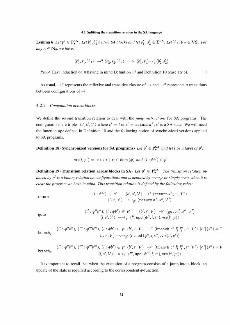
Lemma 6 Let p′ ∈ PSA• . Let b′1, b′2 be two SA blocks and let s′1, s′2 ∈ ΣSA. Let V 1,V 2 ∈ VS . For

any n ∈N0, we have:

〈b′1, s′1,V 1〉 →n 〈b′2, s′2,V 2〉 =⇒ 〈b′1, s′1〉;np 〈b′2, s′2〉

Proof. Easy induction on n having in mind Definition 17 and Definition 10 (case atrib). 2

As usual,→∗ represents the reflexive and transitive closure of→ and→n represents n transitions

between configurations of→.

4.2.2 Computation across blocks

We define the second transition relation to deal with the jump instructions for SA programs. The

configurations are triples 〈c′, s′,V 〉 where c′ = l or c′ = return a ′ , s′ is a SA state. We will need

the function upd defined in Definition 10 and the following notion of synchronized versions applied

to SA programs.

Definition 18 (Synchronized versions for SA programs) Let p′ ∈ PSA• and let l be a label of p′.

vrs(l, p′) = [x 7→ i | xi ∈ dom (φ) and (l : φb′) ∈ p′]

Definition 19 (Transition relation across blocks in SA) Let p′ ∈ PSA• . The transition relation in-

duced by p′ is a binary relation on configurations and is denoted by −◦→p′ or simply −◦→ when it is

clear the program we have in mind. This transition relation is defined by the following rules:

return(l : φb′) ∈ p′ 〈b′, s′,V 〉 →∗ 〈return a ′ , s′′,V ′〉

〈l, s′,V 〉 −◦→p′ 〈return a ′ , s′′,V ′〉

goto(l′ : φ′′b′′), (l : φb′) ∈ p′ 〈b′, s′,V 〉 →∗ 〈goto l′i , s′′,V ′〉

〈l, s′,V 〉 −◦→p′ 〈l′, upd (φ′′, i, s′′), vrs(l′, p)〉

branchT(l′ : φ′′b′′), (l′′ : φ′′′b′′′), (l : φb′) ∈ p′ 〈b′, s′,V 〉 →∗ 〈branch c ′ l′i l′′j , s′′,V ′〉 Jc ′K(s′′) = T

〈l, s′,V 〉 −◦→p′ 〈l′, upd (φ′′, i, s′′), vrs(l′, p′)〉

branchF(l′ : φ′′b′′), (l′′ : φ′′′b′′′), (l : φb′) ∈ p′ 〈b′, s′,V 〉 →∗ 〈branch c ′ l′i l′′j , s′′,V ′〉 Jc ′K(s′′) = F

〈l, s′,V 〉 −◦→p′ 〈l′′, upd (φ′′′, j, s′′), vrs(l′′, p′)〉

It is important to recall that when the execution of a program consists of a jump into a block, an

update of the state is required according to the correspondent φ-function.

32

4.2. Splitting the transition relation in the SA language

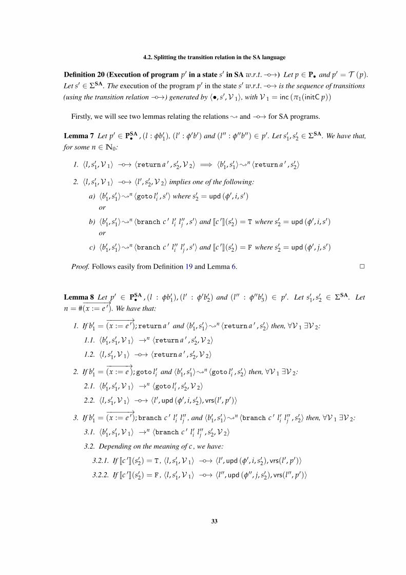
Definition 20 (Execution of program p′ in a state s′ in SA w.r.t.−◦→) Let p ∈ P• and p′ = T (p).Let s′ ∈ ΣSA. The execution of the program p′ in the state s′ w.r.t.−◦→ is the sequence of transitions

(using the transition relation −◦→) generated by 〈•, s′,V 1〉, with V 1 = inc (π1(initC p))

Firstly, we will see two lemmas relating the relations ; and −◦→ for SA programs.

Lemma 7 Let p′ ∈ PSA• , (l : φb′1), (l

′ : φ′b′) and (l′′ : φ′′b′′) ∈ p′. Let s′1, s′2 ∈ ΣSA. We have that,

for some n ∈N0:

1. 〈l, s′1,V 1〉 −◦→ 〈return a ′ , s′2,V 2〉 =⇒ 〈b′1, s′1〉;n 〈return a ′ , s′2〉

2. 〈l, s′1,V 1〉 −◦→ 〈l′, s′2,V 2〉 implies one of the following:

a) 〈b′1, s′1〉;n 〈goto l′i , s′〉 where s′2 = upd (φ′, i, s′)or

b) 〈b′1, s′1〉;n 〈branch c ′ l′i l′′j , s′〉 and Jc ′K(s′2) = T where s′2 = upd (φ′, i, s′)or

c) 〈b′1, s′1〉;n 〈branch c ′ l′′i l′j , s′〉 and Jc ′K(s′2) = F where s′2 = upd (φ′, j, s′)

Proof. Follows easily from Definition 19 and Lemma 6. 2

Lemma 8 Let p′ ∈ PSA• , (l : φb′1), (l

′ : φ′b′2) and (l′′ : φ′′b′3) ∈ p′. Let s′1, s′2 ∈ ΣSA. Let

n = #−−−−−→(x := e ′). We have that:

1. If b′1 =−−−−−→(x := e ′); return a ′ and 〈b′1, s′1〉;n 〈return a ′ , s′2〉 then, ∀V 1 ∃V 2:

1.1. 〈b′1, s′1,V 1〉 →n 〈return a ′ , s′2,V 2〉

1.2. 〈l, s′1,V 1〉 −◦→ 〈return a ′ , s′2,V 2〉

2. If b′1 =−−−−−→(x := e ); goto l′i and 〈b′1, s′1〉;n 〈goto l′i , s′2〉 then, ∀V 1 ∃V 2:

2.1. 〈b′1, s′1,V 1〉 →n 〈goto l′i , s′2,V 2〉

2.2. 〈l, s′1,V 1〉 −◦→ 〈l′, upd (φ′, i, s′2), vrs(l′, p′)〉

3. If b′1 =−−−−−→(x := e ′); branch c ′ l′i l′′j , and 〈b′1, s′1〉;n 〈branch c ′ l′i l′′j , s′2〉 then, ∀V 1 ∃V 2:

3.1. 〈b′1, s′1,V 1〉 →n 〈branch c ′ l′i l′′j , s′2,V 2〉

3.2. Depending on the meaning of c , we have:

3.2.1. If Jc ′K(s′2) = T , 〈l, s′1,V 1〉 −◦→ 〈l′, upd (φ′, i, s′2), vrs(l′, p′)〉

3.2.2. If Jc ′K(s′2) = F , 〈l, s′1,V 1〉 −◦→ 〈l′′, upd (φ′′, j, s′2), vrs(l′′, p′)〉

33

4.2. Splitting the transition relation in the SA language

Proof. The parts 1 are easy inductions on n, and parts 2 follow then from the respective parts 1 and

Definition 19. 2

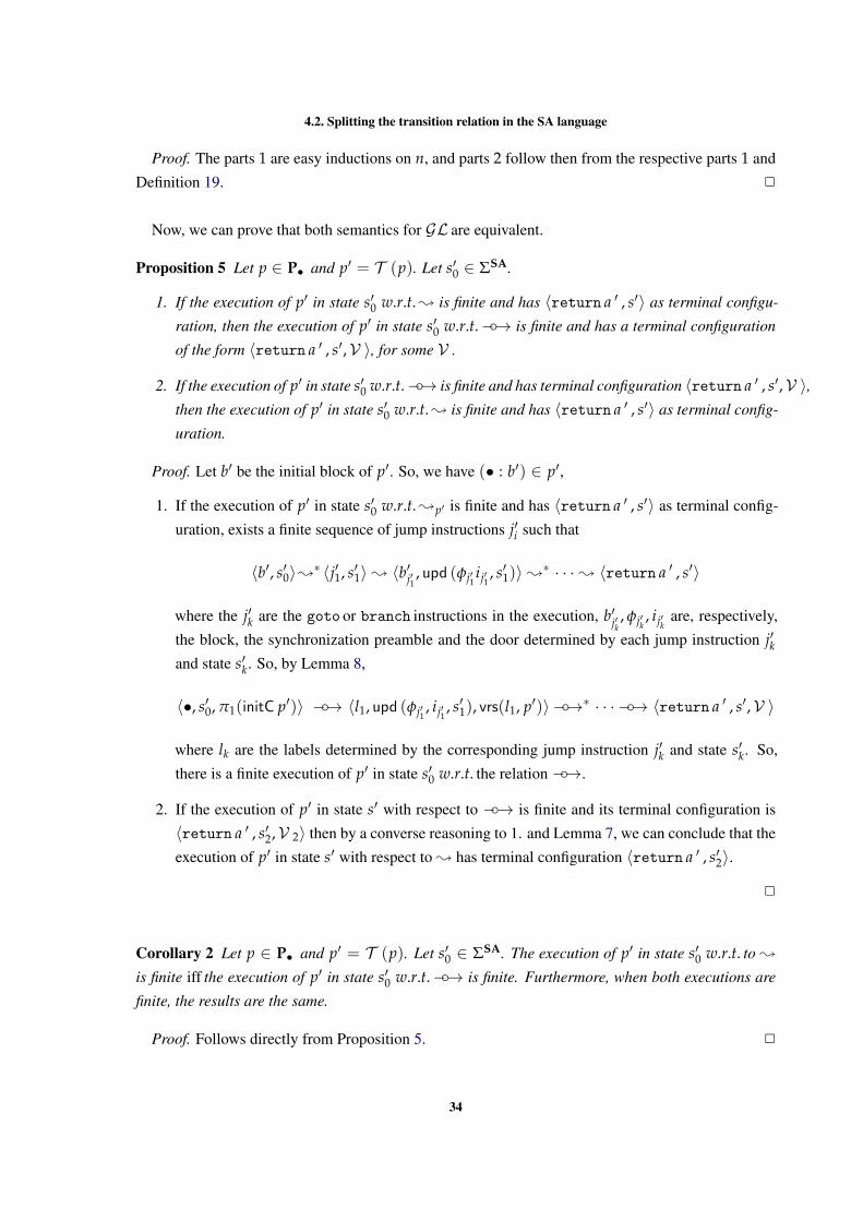
Now, we can prove that both semantics for GL are equivalent.

Proposition 5 Let p ∈ P• and p′ = T (p). Let s′0 ∈ ΣSA.

1. If the execution of p′ in state s′0 w.r.t.; is finite and has 〈return a ′ , s′〉 as terminal configu-

ration, then the execution of p′ in state s′0 w.r.t.−◦→ is finite and has a terminal configuration

of the form 〈return a ′ , s′,V 〉, for some V .

2. If the execution of p′ in state s′0 w.r.t.−◦→ is finite and has terminal configuration 〈return a ′ , s′,V 〉,then the execution of p′ in state s′0 w.r.t.; is finite and has 〈return a ′ , s′〉 as terminal config-

uration.

Proof. Let b′ be the initial block of p′. So, we have (• : b′) ∈ p′,

1. If the execution of p′ in state s′0 w.r.t.;p′ is finite and has 〈return a ′ , s′〉 as terminal config-

uration, exists a finite sequence of jump instructions j′i such that

〈b′, s′0〉;∗ 〈j′1, s′1〉; 〈b′j′1 , upd (φj′1ij′1

, s′1)〉;∗ · · ·; 〈return a ′ , s′〉

where the j′k are the goto or branch instructions in the execution, b′j′k, φj′k

, ij′kare, respectively,

the block, the synchronization preamble and the door determined by each jump instruction j′kand state s′k. So, by Lemma 8,

〈•, s′0, π1(initC p′)〉 −◦→ 〈l1, upd (φj′1, ij′1

, s′1), vrs(l1, p′)〉 −◦→∗ · · · −◦→ 〈return a ′ , s′,V 〉

where lk are the labels determined by the corresponding jump instruction j′k and state s′k. So,

there is a finite execution of p′ in state s′0 w.r.t. the relation −◦→.

2. If the execution of p′ in state s′ with respect to −◦→ is finite and its terminal configuration is

〈return a ′ , s′2,V 2〉 then by a converse reasoning to 1. and Lemma 7, we can conclude that the

execution of p′ in state s′ with respect to ; has terminal configuration 〈return a ′ , s′2〉.

2

Corollary 2 Let p ∈ P• and p′ = T (p). Let s′0 ∈ ΣSA. The execution of p′ in state s′0 w.r.t. to ;

is finite iff the execution of p′ in state s′0 w.r.t.−◦→ is finite. Furthermore, when both executions are

finite, the results are the same.

Proof. Follows directly from Proposition 5. 2

34

4.3. Properties of the translation into SA form

4.3 P RO P E RT I E S O F T H E T R A N S L AT I O N I N T O S A F O R M

In this section we will establish the main properties of our translation T from GL -programs into

SA-programs. We will show soundness and completeness of translation T relatively to the semantic

relations −◦→ of the previous two subsections, i.e. , we will show that a sequence of n steps of the

translated program is mapped to a sequence of n steps in the source program (Theorem 1 and vice-

versa (Theorem 2).

With the help of the soundness and completeness results for T , and the results linking the original

semantics for GL and SA, given by relations ;, with the new semantics for GL and SA in previous

subsection, given by relation −◦→, we will also prove the correctness of T (Theorem 1).

In this subsection we will need the following auxiliary definition and the following lemmas.

Definition 21 (Context in which l is translated) Let p ∈ P• and l ∈ labels(p). The context deter-

mined by the translation of p till label l is given by:

ctx(p, l)=π2(TL (p0, initC p)), for the unique p0 such that p = (p0, l : b , p1), for some b and p1.

As a convention, we say that ctx(p, •) = π1(initC p).

Lemma 9 For e an expression of Aexp or Cexp , s′ ∈ ΣSA, s1 ∈ Σ and V ∈ VS , we have that:

Je K(s1) = JV (e )K(s′ ⊕ V (s1)).

Proof. The proof is made using induction on the structure of expressions. varsE(e) is either an empty

set, a single set or a set of many variables because e can be either a number (which the number of

variables is 0), a single variable (that just have one variable) or a binary expression.

• Case e = n and n ∈N0, varsE(e) is an empty set, immediately we have:

JnK(s1) = nJV (n)K(s′ ⊕ V (s1)) = n

• Case e = x, and x ∈ vars(p), varsE(e) is a single set. We have that:

JxK(s1) = s1(x)JV (x)K(s′ ⊕ V (s1)) = JxV (x)K(s′ ⊕ V (s1)) = s1(x). Note that xV (x) ∈ dom (V (s1)) and

so V (s1)(xV (x)) = s1(x). See Page 21.

• Case e = e 1 op e 2, e 1 and e 2 expressions

Let assume that this lemma is valid for e 1 and e 2. We want to prove that the lemma is also valid

for e 1 op e 2. We have that:

– Je 1K(s1) = JV (e 1)K(s′ ⊕ V (s1))

– Je 2K(s1) = JV (e 2)K(s′ ⊕ V (s1))

35

4.3. Properties of the translation into SA form

We want to prove that: JV (e 1 op e 2)K(s′ ⊕ V (s1)) = Je 1K(s1) op Je 2K(s1)

So,

JV (e 1 op e 2)K(s′ ⊕ V (s1)) = JV (e 1) op V (e 2))K(s′ ⊕ V (s1)) =

JV (e 1)K(s′ ⊕ V (s1)) op JV (e 2)K(s′ ⊕ V (s1)) = Je 1K(s1) op Je 2K(s1)

2

4.3.1 Soundness

We start with some auxiliary functions and two properties about them.

Definition 22 (Erase) The erase function transforms the argument in SA to its counterpart in the

source language. In other words, all indexes and φ-functions are removed. We have that:

• erase (a ′ op a ′′) = erase (a ′) op erase (a ′′)

• erase (return a ′ ) = return (erase (a ′) )

• erase (goto li ) = goto l

• erase (branch c ′ l′i l′′j ) =

branch (erase (c ′) ) l′ l′′

• erase (xi := a ′; b′) =

x := erase (a ′) ; erase (b′)

• erase (φb′) = erase (b′)

• erase (xi) = x

• erase (•) = •

• erase (l) = l

Definition 23 (State restricted to a version function) Let s′ ∈ ΣSA and V ∈ VS . The state s′

restrict to the version function V is represented by s′|V and is the function thats maps each variable

to the correspondent value according to its version in V , that is s′|V (x) = s′(xV (x)), for x ∈ Var.

Lemma 10 Let p ∈ P• and p′ = T (p). Let (l : b) ∈ p and (l : φb′) its counterpart in p′. Let

(V ,L ) = ctx(p, l) and let V ′ and L ′ be such that TB (b, l)(V ,L ) = (b′, (V ′,L ′)). We have that:

erase (b′) = b

Proof. The proof is by induction on the structure of the block b. 2

Lemma 11 Let a ∈ Aexp . Let s′ ∈ ΣSA and V ∈ VS . We have that:

JaK(s′|V ) = JV (a)K(s′)

Proof. The proof is made using induction on the structure of expressions.

• Case a = n and n ∈N,

JnK(s′|V ) = nJV (n)K(s′) = n

36

4.3. Properties of the translation into SA form

• Case a = x and x is a variable,

JxK(s′|V ) = s′|V (x) = s′(xV (x))

JV (x)K(s′) = s′(xV (x))

• Case a = a 1 op a 2,

Let’s assume that the lemma is valid for a 1 and a 2. We have:

1. Ja 1K(s′|V ) = JV (a 1)K(s′)

2. Ja 2K(s′|V ) = JV (a 2)K(s′)

We want to prove that: Ja 1 op a 2K(s′|V ) = JV (a 1 op a 2)K(s′)So,

Ja 1 op a 2K(s′|V ) = s′|V (a 1 op a 2) = s′|V (a 1) op s′|V (s2) = Ja 1K(V ) op Ja 2K(V ) =

JV (a 1)K(s′) op JV (a 2)K(s′) = JV (a 1 op a 2)K(s′)

2

We establish now the basic result to have soundness of the translation relatively to the computations

inside blocks.

Proposition 6 Let p ∈ P• and let p′ in PSA• be such that p′ = T (p). Let (l : b) be a labeled

block in p and (l : φb′) its translation in p′. Let n ∈ N0 and ctx(p, l)=(V ,L ). Let b1 be a part of

b such that b =−−−−→(y := e); b1 and b1 its correspondent translation in p′. Let V 1 be such that V 1 =

inc (V )[−−−−→(y := e)]. LetL 1 be a label function such thatL 1 = L [l 7→ (π1(L (l)), π2(L (l)), inc (V ))].

Let f ′ be a instruction in SA goto l , or return a ′ or branch c ′ l′ l′′ and let V ′,L ′, s′1, s′2 such that:

TB (b1, l)(V 1,L 1) = (b′1, (V ′,L ′)) and 〈b′1, s′1,V 1〉 →np′ 〈 f ′, s′2,V 2〉

Then: 〈b1, s′1|V 1 ,V 1〉 →np 〈erase ( f ′) , s′2|V 2 ,V 2〉

Proof. By induction on n (∈N0).

Base Case, for n=0: We immediately have b′1 = f ′, s′1 = s′2,V 1 = V 2 and:

• erase ( f ′) = f by Lemma 10;

• s′1|V 1 = s′2|V 2 because s′1 = s′2 and V 1 = V 2

Inductive, for n > 0:

Suppose that 〈b′1, s′1, V 1〉 →1 〈b′0, s′0, V 0〉 →n−1 〈 f ′, s′2,V 2〉Because of 〈b′1, s′1, V 1〉 →1 〈b′0, s′0, V 0〉 and Definition17 we have that:

(a) b′1 = (xi := a′); b′0

(b) s′0 = s′1[xi 7→ Ja′K(s′1)]

37

4.3. Properties of the translation into SA form

(c) V 0 = V 1[x 7→ i]

We want to prove that: 〈erase (b′1) , s′1|V 1 , V 1〉 →1 〈erase (b′0) , s′0|V 0 , V 0〉For which we need (by Definition 13):

1. V 0 = V 1[x 7→ V 1(x) + 1]

2. s′0|V 0 = s′1|V 1 [x 7→ Jerase (a′) K(s′1|V 1)]

1. We know that V 0 = V 1[x 7→ i] by (c) above, so we need i = V 1(x) + 1. By Lemma 10, we

have that: b1 = (x := erase (a′) ); erase (b′0) . Furthermore, form definition of TB , we have that

• i = V (x) + 1

• a′ = V 1(erase (a′) ) (*)

2. From (b), (c) and Definition 23 it is enough to prove that

s′1[xi 7→ Ja′K(s′1)]|V 1[x 7→V 1(x)+1] = s′1|V 1 [x 7→ Jerase (a′) K(s′1|V 1)]

Let y ∈ vars(p),

• Case y 6= x,

– s′1[xi 7→ Ja′K(s′1)]|V 1[x 7→V 1(x)+1](y) = s′1(yV 1(y))

– s′1|V 1 [x 7→ Jerase (a′) K(s′1|V 1)](y) = s′1(yV 1(y))

• Case y = x,

– s′1[xi 7→ Ja′K(s′1)]|V 1[x 7→V 1(x)+1](y) = Ja′K(s′1)

– s′1|V 1 [x 7→ Jerase (a′) K(s′1|V 1)](y) = Jerase (a′) K(s′1|V 1)

By (*), Ja′K(s′1) = JV 1(erase (a′) )K(s′1) which is equal to Jerase (a′) K(s′1|V 1) by Lemma 11.

2

The previous result allows us to obtain soundness w.r.t. one step computations across blocks.

Proposition 7 Let p ∈ P• and let p′ in PSA• be such that p′ = T (p). Let l ∈ labels(p), V 1 ∈ VS

and let L 1 = L [l 7→ (π1(L (l)), π2(L (l)), inc (V ))] such that ctx(p, l) = (V 1,L 1). Let

V 0 = inc (V 1). Let f ′ be a instruction in SA goto l , or return a ′ or branch c ′ l′ l′′ and let

s′0, s′2,V 2 such that:

〈l, s′0,V 0〉 −◦→p′ 〈 f ′, s′2,V 2〉 =⇒ 〈l, s′0|V 0 ,V 0〉 −◦→p′ 〈erase ( f ′) , s′2|V 2 ,V 2〉

38

4.3. Properties of the translation into SA form

Proof. Let b be a block labeled by l in p and b′ its translation to SA in p′.

• For f ′ = return a′ , We have that:

〈l, s′0,V 0〉 −◦→p′ 〈return a′ , s′2,V 2〉From Definition 15 follows:

〈b′, s′0,V 0〉 →np′ 〈return a′ , s′2,V 2〉

By Proposition 6 we have 〈b, s′0|V 0 ,V 0〉 →np 〈erase (return a′ ) , s′2|V 2 ,V 2〉

Again, using Definition 15 follows: 〈l, s′0|V 0 ,V 0〉 −◦→p′ 〈erase (return a′ ) , s′2|V 2 ,V 2〉

• For f ′ = l, is analogous.

2

With the help of the previous proposition, we achieve now the soundness of the translation T for

the relations that speak about computations across blocks.

Theorem 1 (Soundness) Let p ∈ P• and let p′ be T (p). Let V 1 = inc (π1(initC p)). For any

s′1, s′2,V 2 and f ′,〈•, s′1,V 1〉 −◦→n

p′ 〈 f ′, s′2,V 2〉 =⇒ 〈•, s′1|V 1 ,V 1〉 −◦→np 〈erase ( f ′) , s′2|V 2 ,V 2〉

Proof. By induction on n ∈N0.

Case n = 0.

We have that: 〈•, s′1,V 1〉 −◦→0p′ 〈 f ′, s′2,V 2〉

And by definition of −◦→ we know that:

• s′1 = s′2

• V 2 = V 1

• f ′ = •

We want to prove that: 〈•, s′1V 1|,V 1〉 −◦→0p 〈erase ( f ′) , s′2|V 2 ,V 2〉, which is immediate since:

• erase ( f ) = erase (•) = •;

• s′1|V 1 = s′2|V 2 because s′2 = s′1 and V 2 = V 1.

Case n ≥ 1

We have that: 〈•, s′1,V 1〉 −◦→n−1p′ 〈l, s′0,V 0)〉 −◦→p′ 〈 f ′, s′2,V 2〉

By IH we have 〈•, s′1|V 1 ,V 1〉 −◦→n−1p 〈l, s′0V 0|,V 0〉.

We now will prove that 〈l, s′0|V 0 ,V 0〉 −◦→p 〈erase ( f ′) , s′2|V 2 ,V 2〉. We also know that:

〈l, s′0,V 0〉 −◦→p′ 〈 f , s′2,V 2〉 and f = return a′ or f = l′. So by applying Proposition 7, we

have that 〈l, s′0|V 0 ,V 0〉 −◦→p 〈 f ′, s′2|V 2 ,V 2〉 with f ′ = erase (return a′ ) or f ′ = l′. 2

39

4.3. Properties of the translation into SA form

4.3.2 Completeness

In this subsection we will present some results culminating with the presentation of Theorem 2, which

establishes the completeness of the translation T into SA form. We will prove in Proposition 8 that

if there is a sequence of n steps from anywhere in a block till the end of that block, then there is an

execution from the same point in the translated block till the end of that block.

Proposition 8 Let p ∈ P• and let p′ in PSA• be such that p′ = T (p). Let (l : b) be a labeled block

in p and (l : φb′) its translation in p′. Let n ∈ N0 and ctx(p, l)=(V ,L ). Let b1 be a part of b such

that b =−−−−→(y := e); b1. Let V 1 be such that V 1 = inc (V )[

−−−−→(y := e)]. Let L 1 be a label function such

that L 1 = L [l 7→ (π1(L (l)), π2(L (l)), inc (V ))]. Let f be a instruction goto l , or return a or

branch c l′ l′′ and let b′1,V ′,L ′, s1, s2,V 2 such that:

TB (b1, l)(V 1,L 1) = (b′1, (V ′,L ′)) and 〈b1, s1,V 1〉 →n 〈 f , s2,V 2〉

Then, V ′ = V 2 and:

• If f = return a ,

1. L ′ = L 1

2. ∀s ∈ ΣSA, ∃s′ ∈ ΣSA : 〈b′1, s⊕ V 1(s1),V 1〉 →n 〈return V 2(a ) , s′ ⊕ V 2(s2),V 2〉

• If f = goto l′ ,

1. L ′ = L 1[l′ 7→ (π1L 1(l′) + 1, π2L 1(l′) ++ [V ′], π3L 1(l′))]

2. ∀s ∈ ΣSA, ∃s′ ∈ ΣSA : 〈b′1, s⊕ V 1(s1),V 1〉 →n 〈goto l′π1(L ′(l′))

, s′ ⊕ V 2(s2),V 2〉

• If f = branch c l′ l′′ ,

1. L 2 = L 1[l′ 7→ (n′ + 1, d′ ++ [V 1],V ′0)] where (n′, d′,V ′0) = L 1(l′) and

L ′ = L 2[l′′ 7→ (n′′ + 1, d′′ ++ [V 1],V ′′0 )] where (n′′, d′′,V ′′0 ) = L 2(l′′)

2. ∀s ∈ ΣSA, ∃s′ ∈ ΣSA :〈b′1, s⊕ V 1(s1),V 1〉 →n 〈branch V 2(c ) l′

π1(L ′(l′))l′′π1(L ′(l′′))

, s′ ⊕ V 2(s2),V 2〉

Proof. By induction on n (∈N0).

Base Case, for n=0: We immediately have b1 = f , s1 = s2,V 1 = V 2 and by inspection of TB we

see that V ′ = V 1 = V 2.

• If f = return a ,

1. Inspection of TB gives immediately L ′ = L 1

2. Also, we have:

– b1 = return a

40

4.3. Properties of the translation into SA form

– b′1 = return V 1(a )

We want to prove that: ∀s∃s′ : 〈b′1, s⊕V 1(s1),V 1〉 →0 〈return V 2(a ) , s′⊕V 2(s2),V 2〉So, it suffices to take s′ = s, since V 1 = V 2 and s1 = s2.

• If f = goto l′ ,

1. Inspection of TB and the fact that V ′ = V 1 gives

L ′ = L 1[l′ 7→ (π1L 1(l′) + 1, π2L 1(l′) ++ [V ′], π3L 1(l′))]

2. Also, we have:

– b1 = goto l′

– b′1 = goto l′π1(L ′(l′))+1

We want to prove that 〈b′1, s⊕ V 1(s1),V 1〉 →0 〈goto l′π1(L ′(l′))

, s′ ⊕ V 2(s2),V 2〉So, it suffices to take s′ = s since V 1 = V 2 and s1 = s2.

• If f = branch c l′ l′′ ,

1. Let L 2 = L 1[l′ 7→ (n′ + 1, d′ ++ [V 1],V ′0)] where (n′, d′,V ′0) = L 1(l′). By inspec-

tion of TB and the fact that V ′ = V 1 we have:

L ′ = L 2[l′′ 7→ (n′′ + 1, d′′ ++ [V 1],V ′′0 )] where (n′′, d′′,V ′′0 ) = L 2(l′′)

2. Also, we have:

– b1 = branch c l′ l′′

– b′1 = branch V 1(c ) l′n′+1 l′′n′′+1

We want to prove that ∀s∃s′ such that

〈b′1, s⊕ V 1(s1),V 1〉 →0 〈branch V 2(c ) l′π1(L ′(l′))

l′′π1(L ′(l′′))

, s′ ⊕ V 2(s2),V 2〉It suffices to take s′ = s since V 1 = V 2, s1 = s2 and

branch V 1(c ) l′n′+1 l′′n′′+1 = branch V 2(c ) l′π1(L ′(l′))

l′′π1(L ′(l′′))

because:

– V 1 = V 2

– π1(L ′(l′)) = n′ + 1

– π1(L ′(l′′)) = n′′ + 1

Inductive Case, for n > 0:

Suppose that 〈b1, s1,V 1〉 →1 〈b0, s0,V 0〉 →n−1 〈 f , s2,V 2〉Because of 〈b1, s1,V 1〉 →1 〈b0, s0,V 0〉, we have that:

• b1 = (x := a 0); b0, for some x and a 0

• s0 = s1[x 7→ Ja 0K(s1)] (*)

• V 0 = V 1[x 7→ V 1(x) + 1] (**)

41

4.3. Properties of the translation into SA form

• TB (b1, l)(V 1,L 1) = (xV 1(x)+1 := V 1(a 0); b′0, (V ′,L ′))where (b′0, (V ′,L ′)) = TB (b0, l)(V 0,L 1)

We have:

• b = (−−−→y := e ) ++ x := a0; b0 (recall b =−−−−−→(y := e ); b1 and b1 = x := a 0; b0) (1)

• TB (b0, l)(V 0,L 1) = (b′0, (V ′,L ′)) (2)

• 〈b0, s0,V 0〉 →n−1 〈 f , s2,V 2〉 (3)

• V 0 = inc (V )[(−−−→y := e ) ++ x := a0] because V 1 = inc (V )[(−−−→y := e )] and (**) (4)

Because of (1), (2), (3) and (4) we can use the IH to conclude that V ′ = V 2.

– If f = return a ,

1. From the IH, we can conclude that L ′ = L 1

2. From the IH, we can also conclude that:

∀s∃s′: (5)

〈b′0, s⊕∧

V 1[x 7→ V 1(x) + 1](s1[x 7→ Ja 0K(s1)]),V 0〉 →n−1 〈return V 2(a ) , s′⊕V 2(s2),V 2〉

Recall the equalities on (*) and (**).

For a fixed s ∈ ΣSA: (6)

〈xV 1(x)+1 := V 1(a 0); b′0, s⊕ V 1(s1),V 1〉 →〈b′0, s⊕ V 1(s1)[xV 1(x)+1 7→ JV 1(a 0)K(s⊕ V 1(s1))],V 1[x 7→ V 1(x) + 1]〉

Fix s ∈ ΣSA. Because of (6) and (5), it suffices to prove that:

s⊕ V 1(s1)[xV 1(x)+1 7→ JV 1(a 0)K(s⊕ V 1(s1))] = (7)

s⊕∧

V 1[x 7→ V 1(x) + 1](s1[x 7→ Ja 0K(s1)])

and V 1[x 7→ V 1(x) + 1] = V 0.The latter is given by (**). Also, we can prove that:

V 1(s1)[xV 1(x)+1 7→ JV 1(a 0)K(s⊕ V 1(s1))] =

∧

V 1[x 7→ V 1(x) + 1](s1[x 7→ Ja 0K(s1)])

It is easy to see that the right hand side and left hand side assign the same values to

variables distinct of xV (x)+1. For xV 1(x)+1, the left hand side state and the right hand side

state assign the values JV 1(a 0)K(s⊕ V 1(s1)) and Ja 0K(s1), which are equal by Lemma 9.

42

4.3. Properties of the translation into SA form

– f = goto l or f = branch c l′ l′′

The argument is analogous to the previous one. For example, if f = goto l ,

1. We can use the IH to conclude that

L ′ = L 1[l′ 7→ (π1L 1(l′) + 1, π2L 1(l′) ++ [V ′], π3L 1(l′))]

2. We can use the IH to also conclude that:

〈b′0, s⊕∧

V 1[x 7→ V 1(x) + 1](s1[x 7→ Ja 0K(s1)]),V 0〉 →n−1 〈goto lπ1(L ′(l′)) , s′⊕V 2(s2),V 2〉

so it suffices to prove (7), which we have already proved in the previous case.

2

In Proposition 9 we will establish a property analogous to the one in the previous proposition,

Proposition 8, but now dealing with the relation −◦→.

Proposition 9 Let p ∈ P• and let p′ in PSA• be such that p′ = T (p). Let l be a label of p. Let

V 1 ∈ VS be such that ctx(l, p) = (V 1,L 1).

Let s1, s2,V 2 be such that 〈l, s1, inc (V 1))〉 −◦→p 〈return a , s2,V 2〉 (*)

we have, ∀s∃s′, 〈l, s⊕ inc (V 1)(s1), inc (V 1)〉 −◦→p′ 〈return V 2(a ) , s′ ⊕ V 2(s2),V 2〉

Proof. Let b be the block labeled by l in p and (l : φb′) its translation in p′.LetL ′1 = L 1[l 7→ (π1L 1(l), π2L 1(l), inc (V 1))] and let TB (b, l)(inc (V 1),L ′1) = (b′, (V 0,L 0))

From assumption (*) and Definition 15, we have that

〈b, s1, inc (V 1)〉 →∗ 〈return a , s2,V 2〉.So, by applying Proposition 8(part 2, case return), we have

∀s∃s′, 〈b′, s⊕ inc (V 1)(s1), inc (V 1)〉 →n 〈return V 2(a ) , s′ ⊕ V 2(s2),V 2〉.Using Definition 19 follows: 〈l, s⊕ inc (V 1)(s1), inc (V 1)〉 −◦→p′ 〈return V 2(a ) , s′⊕V 2(s2),V 2〉2

We continue now with a lemma used in the proof of Proposition 10. Proposition 10 ensures that

if a transition is made and execution moves to another block, then in the correspondent translated

program, this execution is also possible.

Lemma 12 Let p ∈ P• and l, l′ ∈ labels(p). Let us have ctx(p, l) = (V ,L ).

#(π2(L (l′)) = π1(L (l′))

Proof. Follows from the Definition 21 and by analyzing inductively the function TL . 2

43

4.3. Properties of the translation into SA form

Proposition 10 Let p ∈ P• and let p′ in PSA• be such that p′ = T (p). Let l, l′ ∈ labels(p). Let

(l : b) and (l′ : b′) be labeled blocks in p and (l : φb0) and (l′ : φ′b1) be their translations in p′. Let

ctx(p, l) = (V 1,L 1). Let s1, s2 and V 2 be such that: 〈l, s1, inc (V 1)〉 −◦→p 〈l′, s2,V 2〉.Then, ∀s∃s′, 〈l, s⊕ inc (V 1)(s1), inc (V 1)〉 −◦→p′ 〈l′, s′ ⊕ V 2(s2),V 2〉

Proof. The proof will be by case analysis in the constitution of b, in particular in the last instruc-

tion of b. Let L 2 = L 1[l 7→ (π1L 1(l), π2L 1(l), inc (V 1))] and let TB (b, l)(inc (V 1),L 2) =

(b0, (V ′,L ′)), for some V ′ and L ′.

• Case b has the form−−−−→(y := a); goto l′ .

Let s be an arbitrary state. From 〈l, s1, inc (V 1)〉 −◦→p 〈l′, s2,V 2〉 we know that (by Defini-

tion 15), for some n and some V 3, 〈b, s1, inc (V 1)〉 →np 〈goto l′ , s2,V 3〉 and V 2 = vrs(l′, p).

By Proposition 8, we have that V ′ = V 3.

Also, by Proposition 8 (part 1, case goto) we have that:

– L ′ = L 2[l′ 7→ (π1L 2(l′) + 1, π2L 2(l′) ++ [V 3], π3L 2(l′))])

From this, using Proposition 8 (part 2, case goto), we have that

〈b0, s⊕ inc (V 1)(s1), inc (V 1)〉 →∗ 〈goto l′π1(L ′(l′))

, s′ ⊕ V 3(s2),V 3〉, for some s′′. Hence,

by the goto rule from Definition 19,

〈l, s⊕ inc (V 1)(s1), inc (V 1)〉 −◦→p′ 〈l′, upd (φ′, π1(L ′(l′)), s′ ⊕ V 3(s2)), vrs(l′, p′)〉. So,

we just have to prove that upd (φ′, π1(L ′(l′)), s′ ⊕ V 3(s2)) = s′ ⊕ V 2(s2), for some s′, and

vrs(l′, p′) = vrs(l′, p) = V . The latter is immediate since p′ = T (p). We will now show the

former holds for s′ = s′′ ⊕ V 3(s2)

Let s∗ = upd (φ′, π1(L ′(l′)), s′ ⊕ V 3(s2)) and by Definition 10, we have that

s∗ = s′ ⊕ V 3(s2)[xi 7→ J−→x [π1(L ′(l′))]K(s′ ⊕ V 3(s2)) | xi := φ(−→x ) ∈ φ′]

Let yj ∈ VarSA

– Case yj 6∈ dom (φ′) and V 3(y) = j.s∗(yj) = V 3(s2)(yj) = s2(y)We want to show that s2(y) = (s′ ⊕ V 2(s2))(yj)

As y2 6∈ dom (φ′) and V 2 = vrs(l′, p), s2(y) = s′(yj)

How s′ = s′′ ⊕ V 3(s2), s′(yj) = (s′′ ⊕ V 3)(s2)(yj) = s2(yj)

– Case yj 6∈ dom (φ′) and V 3(y) 6= js∗(yj) = s′(yj).

We want to show that s′(yj) = s′ ⊕ V 2(s2)(yj)

This is true because V 2 = vrs(l′, p) and yj 6∈ dom (φ′).

– Case yj ∈ dom (φ′), i.e. , yj := φ(−→y ) ∈ φ′

Let n = π1(L ′(l′)),

44

4.3. Properties of the translation into SA form

s∗(yj) = J−→y [n]K(s′ ⊕ V 3(s2))

= (s′ ⊕ V 3(s2))(yW(y)), with W = π2(L ′(l′))[n](by definition of sync)

= (s′ ⊕ V 3(s2)(yV 3(y)) (W = V 3, which follows by Lemma 12)

= s2(y) (From the definition of ⊕ and ˆ operators.)

Hence, we can conclude that upd (φ′, π1(L ′(l′)), s′ ⊕ V 3(s2)) = s′ ⊕ V 2(s2)

Now, we want to show that s2(y) = s′ ⊕ V 2(s2)(yj). This is true because V 2(y) = j,since vrs(l, p) = V 2 by Definition 14 and yj ∈ dom (φ′). For the yj 6∈ dom (φ′), as

s′ = s′′ ⊕ V 3(s2), this is also proved.

• Case b has the form−−−−→(y := a); branch c l′ l′′

This case is analogous to the previous one.

2

We now present two more lemmas (Lemma 13 and Lemma 14) and we bring forward a main

theorem. This theorem will prove the completeness of our translation.

Lemma 13 Let p ∈ P• and l ∈ labels(p). We have that:

vrs(l, p) = inc (π1(ctx(p, l)))

Proof. The lemma follows from Definition 14 and Definition 21, and by inspecting the translation

function T , in what concerns the construction of the synchronization blocks φ . 2

Lemma 14 Let p ∈ P• . Let V 1 = inc (π1(initC p))For any n ≥ 1, s1, s2, l and V 2 we have that 〈•, s1,V 1〉 −◦→n

p 〈l, s2,V 2〉 =⇒ V 2 = inc (π1ctx(p, l)).

Proof. Assume 〈•, s1,V 1〉 −◦→n−1p 〈l′, s3,V 3〉 −◦→p 〈l, s2,V 2〉, where in the case n = 1 we

have that l′ = •, s1 = s3 and V 1 = V 3.

We want to prove that inc (π1ctx(p, l)) = V 2

Inspecting Definition 15, we see that V 2 = vrs(l, p). Hence, using Lemma 13, V 2 = inc (π1ctx(p, l)).2

Theorem 2 (Completeness) Let p ∈ P• and let p′ be T (p). Let V 1 = inc (π1(initC p)). For any

n, s1, s2,V 2, f ,

〈•, s1,V 1〉 −◦→np 〈 f , s2,V 2〉 =⇒ ∀s∃s′, 〈•, s⊕ V 1(s1),V 1〉 −◦→n

p′ 〈V 2( f ), s′ ⊕ V 2(s2),V 2〉

45

4.3. Properties of the translation into SA form

Proof. By induction on n ∈N0.

Case n = 0.

We have that: 〈•, s1, inc (V 1)〉 −◦→0p 〈 f , s2,V 2〉

So, we know that:

• s1 = s2

• V 2 = inc (V 1)

• f = •

We want to prove that: ∀s∃s′, 〈•, s⊕ V 1(s1),V 1〉 −◦→0p′ 〈V 2( f ), s′ ⊕ V 2(s2),V 2〉, which is im-

mediate since V 2( f ) = V 2(•) = • and then we just have to take s′ = s.

Case n ≥ 1

We have that: 〈•, s1,V 1〉 −◦→n−1p 〈l, s0,V 0〉 −◦→p 〈 f , s2,V 2〉. Let s be an arbitrary state.

By IH we have 〈•, s⊕ V 1(s1),V 1〉 −◦→n−1p 〈l, s′′ ⊕ V 0)(s0),V 0〉, for some s′′. We now will

prove that 〈l, s′′ ⊕ V 0(s0),V 0〉 −◦→p′ 〈V 2( f ), s′ ⊕ V 2(s2),V 2〉 for some s′.

1. Case f = return a .

By Lemma 14 we have that V 0 = inc (π1(ctx(p, l))). We also know that:

〈l, s0,V 0〉 −◦→p 〈return a , s2,V 2〉So by applying Proposition 9, we have that for some s′

〈l, s′′ ⊕ V 0(s0),V 0〉 −◦→p′ 〈return V 2(a ) , s′ ⊕ V 2(s2),V 2〉.

2. Case f = l′,Again, by Lemma 14 we have that V 0 = inc (π1(ctx(p, l))). We also know that:

〈l, s0,V 0〉 −◦→p 〈l′, s2,V 2〉So by applying Proposition 10, we have that 〈l, s′⊕ V 0(s0),V 0〉 −◦→p′ 〈l′, s′⊕ V 2(s2),V 2〉,for some s′.

2

4.3.3 Correctness

Finally, we can establish the correctness of the translation T into SA form. This is achieved by

combining the soundness and completeness results of the previous subsections, but also using the

equivalence of the alternative semantics we introduced both for SA and GL .

Theorem 3 (Correctness of the translation into SA form) Let p ∈ P• and let p′ = T (p). Let

s ∈ Σ and let s′, s′′ ∈ ΣSA be such that s′ = s′′ ⊕∧

inc (π1(initC p))(s).

46

4.3. Properties of the translation into SA form

The execution of p in state s is finite iff the execution of p′ in state s′ if finite. Furthermore, if both

executions are finite, the results of both executions are the same.

Proof. The first statement follows from Proposition 4, Proposition 5, Theorem 2 and Theorem 1 we

give only details of the proof of the second statement which requires similar ideas:

1. Assume the execution of p in state s w.r.t.; is finite and its terminal configuration is 〈return a , s2〉and so the result of the execution is Ja K(s2). By Proposition 4, the execution of p in state sw.r.t.−◦→ is finite and gives a terminal configuration 〈return a , s2,V 2〉 for some V 2. There-

fore, by Theorem 2, the execution of p′ in state s′ w.r.t.−◦→ produces a terminal configuration

〈return V 2(a ) , s′′′ ⊕ V 2(s2),V 2〉, for some s′′′. Hence, by Proposition 5, the execution of

p′ in state s′ w.r.t.; produces terminal configuration 〈return V 2(a ) , s′′′ ⊕ V 2(s2)〉 and its

return value is JV 2(a )K(s′′′ ⊕ V 2(s2)), which is equal to Ja K(s2) by Lemma 9, as we wanted

to show.

2. The converse has similar details but using Theorem 1 instead of Theorem 2.

2

47

5

F I NA L R E M A R K S

This chapter concludes the thesis. We begin by analyzing some possible improvements to our SA

translation function, T . Then we discuss the relation between the programs obtained by the transla-

tion function and functional programs. Finally we present some conclusions and future work.

5.1 S A T R A N S L AT I O N

As we saw, the conversion of programs with jumps is done with the help of a notational trick, the φ-

functions. They are used to somehow merge possible different values of a variable at the joint points

of the CFG. For instance, in some node with two incoming edges (doors), the expression φ(x1, x2)

has the value of x1 if the node is reached on the first in-edge, and of x2 if the node is reached on the

second in-edge.

In Chapter 3 we have implemented a naive SA translation with obvious possible improvements.

We choose to work with a naive version to begin with, because our focus was to prove its correction

with respect to the structural operational semantics, and we anticipate that it would be a very intricate

proof.

In our naive translation we choose synchronize every variable of the program at the beginning of

each block, even if the block has a sole in-edge. So, for a program with n blocks and m variables, our

translation produces n×m new assignments.

5.1.1 Optimal placement of φ-functions

There are obvious optimizations to our translation. For instance, we would not need to place φ-

functions in nodes with a sole in-edge.

A tempting but erroneous optimization is to synchronize only variables used in the block. This is

wrong because when two different definitions of a variable reach a node, even if this variable is not

used in that block, it can be used in the subsequent nodes and so one needs to know which is the value

of the variable, and for that we need to synchronize it with a φ-function.

48

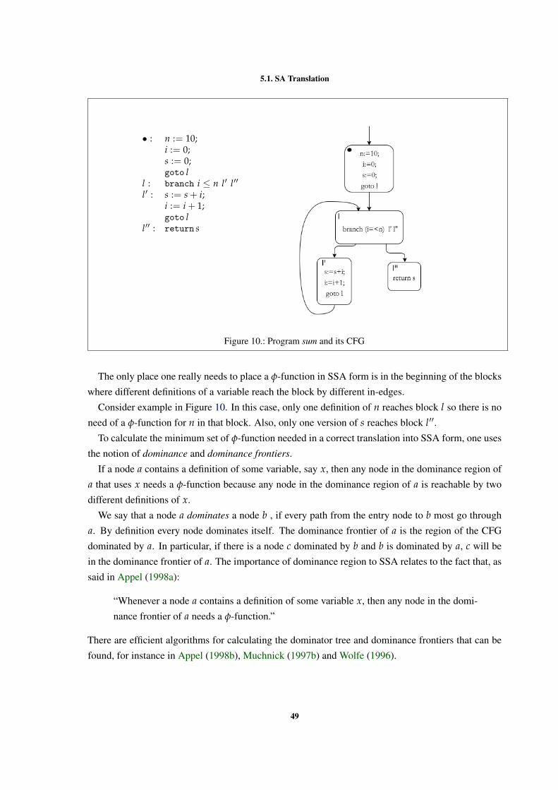
5.1. SA Translation

• : n := 10;i := 0;s := 0;goto l

l : branch i ≤ n l′ l′′

l′ : s := s + i;i := i + 1;goto l

l′′ : return s

Figure 10.: Program sum and its CFG

The only place one really needs to place a φ-function in SSA form is in the beginning of the blocks

where different definitions of a variable reach the block by different in-edges.

Consider example in Figure 10. In this case, only one definition of n reaches block l so there is no

need of a φ-function for n in that block. Also, only one version of s reaches block l′′.To calculate the minimum set of φ-function needed in a correct translation into SSA form, one uses

the notion of dominance and dominance frontiers.

If a node a contains a definition of some variable, say x, then any node in the dominance region of

a that uses x needs a φ-function because any node in the dominance region of a is reachable by two

different definitions of x.

We say that a node a dominates a node b , if every path from the entry node to b most go through

a. By definition every node dominates itself. The dominance frontier of a is the region of the CFG

dominated by a. In particular, if there is a node c dominated by b and b is dominated by a, c will be

in the dominance frontier of a. The importance of dominance region to SSA relates to the fact that, as

said in Appel (1998a):

“Whenever a node a contains a definition of some variable x, then any node in the domi-

nance frontier of a needs a φ-function.”

There are efficient algorithms for calculating the dominator tree and dominance frontiers that can be

found, for instance in Appel (1998b), Muchnick (1997b) and Wolfe (1996).

49

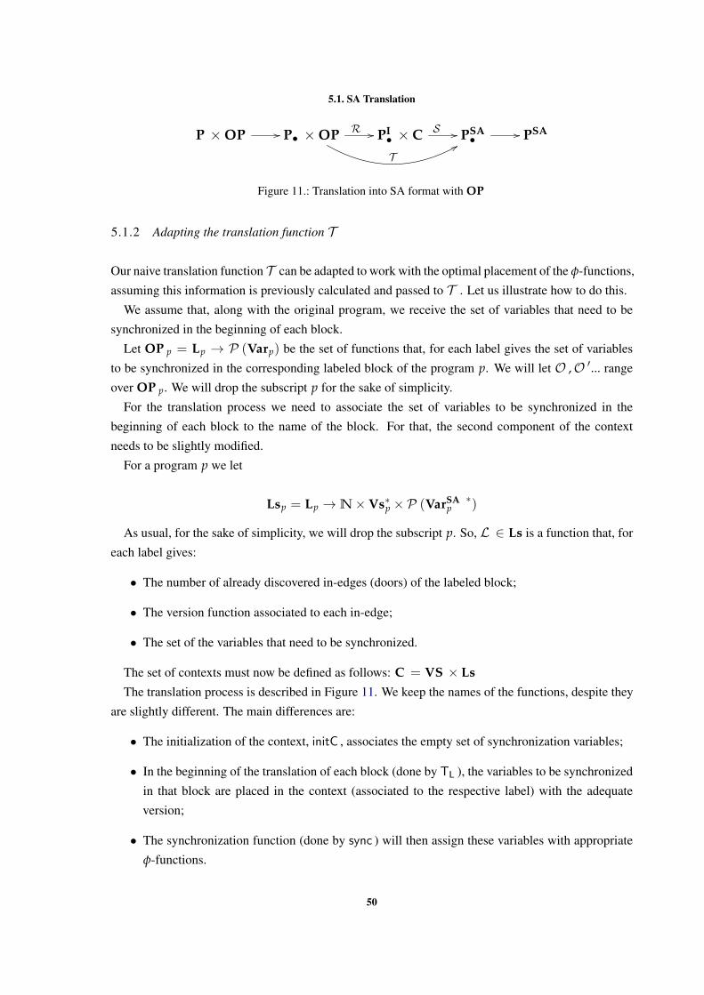
5.1. SA Translation

P ×OP // P• ×OP R //

T88

PI• × C S // PSA

• // PSA

Figure 11.: Translation into SA format with OP

5.1.2 Adapting the translation function T

Our naive translation function T can be adapted to work with the optimal placement of the φ-functions,

assuming this information is previously calculated and passed to T . Let us illustrate how to do this.

We assume that, along with the original program, we receive the set of variables that need to be

synchronized in the beginning of each block.

Let OP p = Lp → P (Varp) be the set of functions that, for each label gives the set of variables

to be synchronized in the corresponding labeled block of the program p. We will let O ,O ′... range

over OP p. We will drop the subscript p for the sake of simplicity.

For the translation process we need to associate the set of variables to be synchronized in the

beginning of each block to the name of the block. For that, the second component of the context

needs to be slightly modified.

For a program p we let

Lsp = Lp →N×Vs∗p ×P (VarSAp )∗)

As usual, for the sake of simplicity, we will drop the subscript p. So, L ∈ Ls is a function that, for

each label gives:

• The number of already discovered in-edges (doors) of the labeled block;

• The version function associated to each in-edge;

• The set of the variables that need to be synchronized.

The set of contexts must now be defined as follows: C = VS × LsThe translation process is described in Figure 11. We keep the names of the functions, despite they

are slightly different. The main differences are:

• The initialization of the context, initC , associates the empty set of synchronization variables;

• In the beginning of the translation of each block (done by TL ), the variables to be synchronized

in that block are placed in the context (associated to the respective label) with the adequate

version;

• The synchronization function (done by sync ) will then assign these variables with appropriate

φ-functions.

50

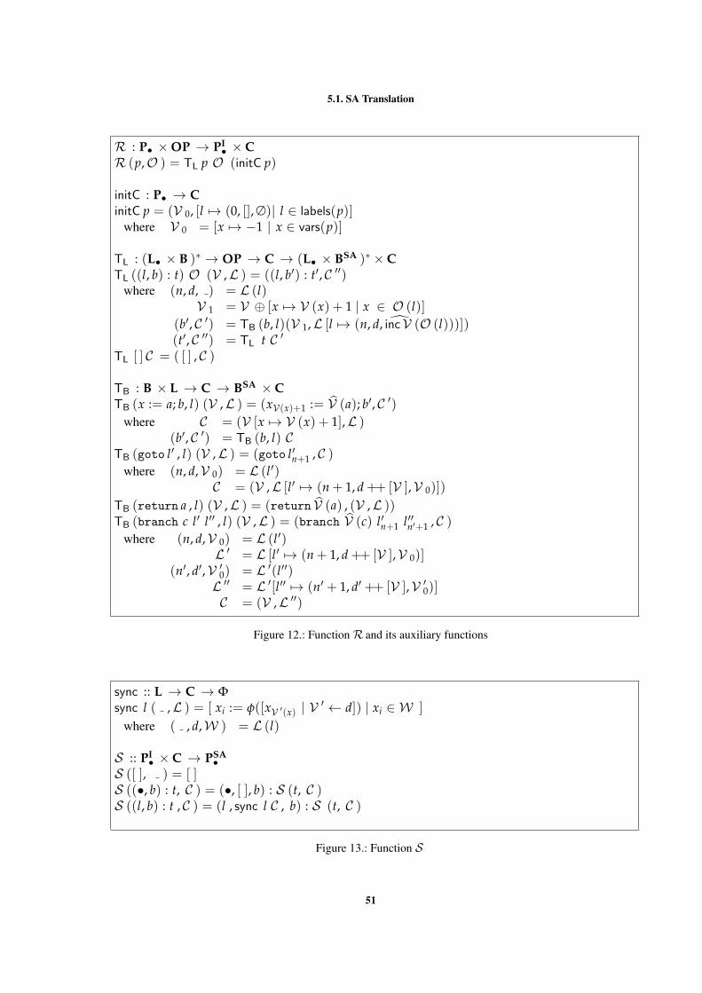
5.1. SA Translation

R : P• ×OP → PI• × C

R (p,O ) = TL p O (initC p)

initC : P• → CinitC p = (V 0, [l 7→ (0, [], ∅)| l ∈ labels(p)]

where V 0 = [x 7→ −1 | x ∈ vars(p)]

TL : (L• × B )∗ → OP → C → (L• × BSA )∗ × CTL ((l, b) : t) O (V ,L ) = ((l, b′) : t′, C ′′)

where (n, d, ) = L (l)V 1 = V ⊕ [x 7→ V (x) + 1 | x ∈ O (l)]

(b′, C ′) = TB (b, l)(V 1,L [l 7→ (n, d, incV (O (l)))])(t′, C ′′) = TL t C ′

TL [ ] C = ( [ ] , C )

TB : B × L → C → BSA × CTB (x := a; b, l) (V ,L ) = (xV(x)+1 := V (a); b′, C ′)

where C = (V [x 7→ V (x) + 1],L )(b′, C ′) = TB (b, l) C

TB (goto l′ , l) (V ,L ) = (goto l′n+1 , C )where (n, d,V 0) = L (l′)

C = (V ,L [l′ 7→ (n + 1, d ++ [V ],V 0)])

TB (return a , l) (V ,L ) = (return V (a) , (V ,L ))TB (branch c l′ l′′ , l) (V ,L ) = (branch V (c) l′n+1 l′′n′+1 , C )

where (n, d,V 0) = L (l′)L ′ = L [l′ 7→ (n + 1, d ++ [V ],V 0)]

(n′, d′,V ′0) = L ′(l′′)L ′′ = L ′[l′′ 7→ (n′ + 1, d′ ++ [V ],V ′0)]C = (V ,L ′′)

Figure 12.: FunctionR and its auxiliary functions

sync :: L → C → Φsync l ( ,L ) = [ xi := φ([xV ′(x) | V ′ ← d]) | xi ∈ W ]

where ( , d,W ) = L (l)

S :: PI• × C → PSA

•S ([ ], ) = [ ]S ((•, b) : t, C ) = (•, [ ], b) : S (t, C )S ((l, b) : t , C ) = (l , sync l C , b) : S (t, C )

Figure 13.: Function S

51

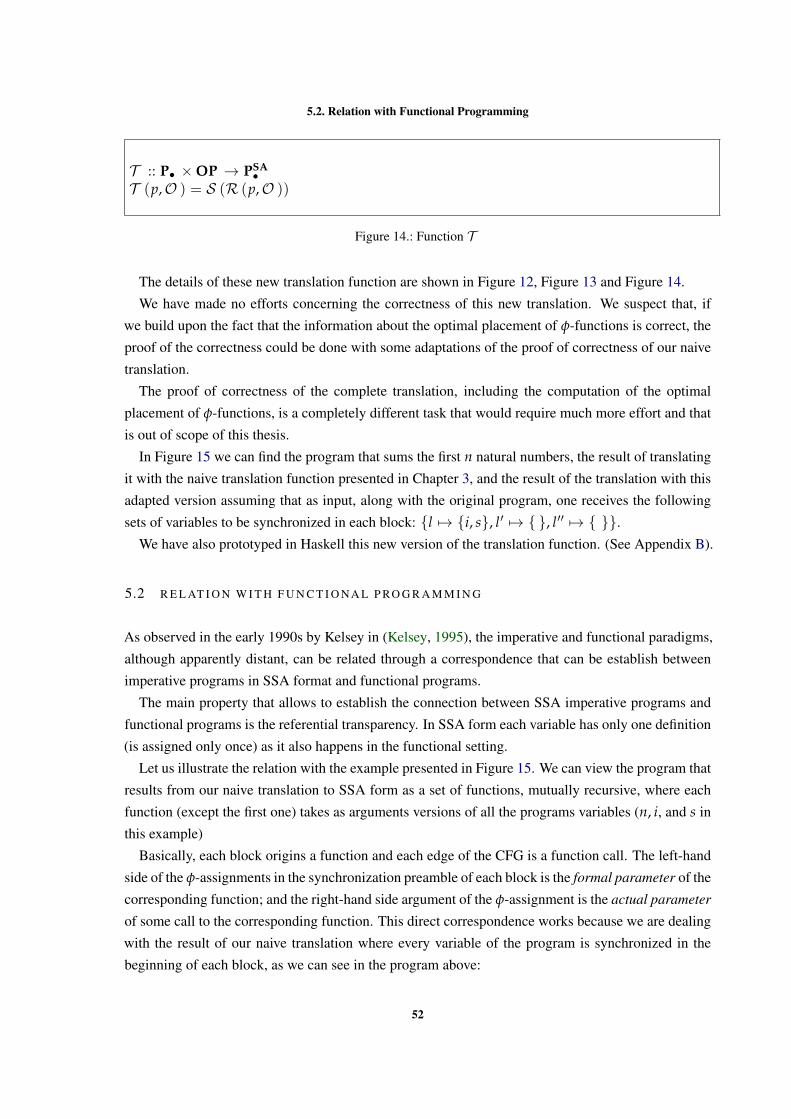
5.2. Relation with Functional Programming

T :: P• ×OP → PSA•

T (p,O ) = S (R (p,O ))

Figure 14.: Function T

The details of these new translation function are shown in Figure 12, Figure 13 and Figure 14.

We have made no efforts concerning the correctness of this new translation. We suspect that, if

we build upon the fact that the information about the optimal placement of φ-functions is correct, the

proof of the correctness could be done with some adaptations of the proof of correctness of our naive

translation.

The proof of correctness of the complete translation, including the computation of the optimal

placement of φ-functions, is a completely different task that would require much more effort and that

is out of scope of this thesis.

In Figure 15 we can find the program that sums the first n natural numbers, the result of translating

it with the naive translation function presented in Chapter 3, and the result of the translation with this

adapted version assuming that as input, along with the original program, one receives the following

sets of variables to be synchronized in each block: {l 7→ {i, s}, l′ 7→ { }, l′′ 7→ { }}.We have also prototyped in Haskell this new version of the translation function. (See Appendix B).

5.2 R E L AT I O N W I T H F U N C T I O N A L P RO G R A M M I N G

As observed in the early 1990s by Kelsey in (Kelsey, 1995), the imperative and functional paradigms,

although apparently distant, can be related through a correspondence that can be establish between

imperative programs in SSA format and functional programs.

The main property that allows to establish the connection between SSA imperative programs and

functional programs is the referential transparency. In SSA form each variable has only one definition

(is assigned only once) as it also happens in the functional setting.

Let us illustrate the relation with the example presented in Figure 15. We can view the program that

results from our naive translation to SSA form as a set of functions, mutually recursive, where each

function (except the first one) takes as arguments versions of all the programs variables (n, i, and s in

this example)

Basically, each block origins a function and each edge of the CFG is a function call. The left-hand

side of the φ-assignments in the synchronization preamble of each block is the formal parameter of the

corresponding function; and the right-hand side argument of the φ-assignment is the actual parameter

of some call to the corresponding function. This direct correspondence works because we are dealing

with the result of our naive translation where every variable of the program is synchronized in the

beginning of each block, as we can see in the program above:

52

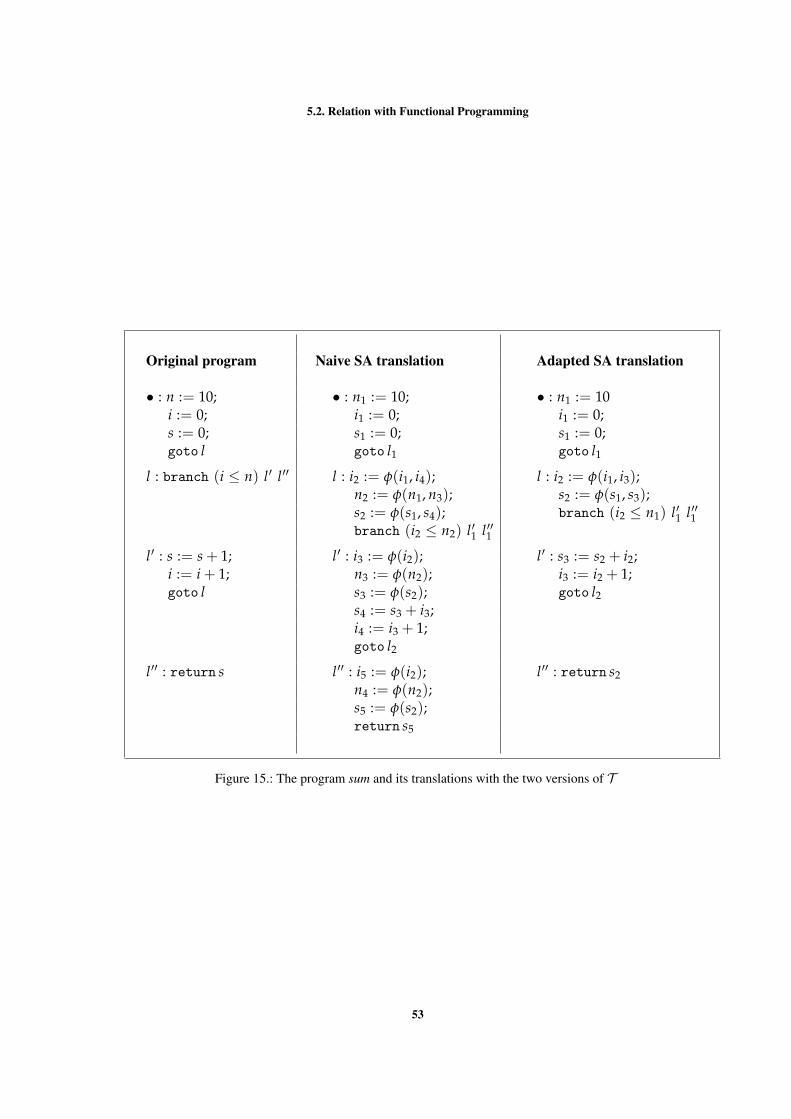
5.2. Relation with Functional Programming

Original program Naive SA translation Adapted SA translation

• : n := 10; • : n1 := 10; • : n1 := 10i := 0; i1 := 0; i1 := 0;s := 0; s1 := 0; s1 := 0;goto l goto l1 goto l1

l : branch (i ≤ n) l′ l′′ l : i2 := φ(i1, i4); l : i2 := φ(i1, i3);n2 := φ(n1, n3); s2 := φ(s1, s3);s2 := φ(s1, s4); branch (i2 ≤ n1) l′1 l′′1branch (i2 ≤ n2) l′1 l′′1

l′ : s := s + 1; l′ : i3 := φ(i2); l′ : s3 := s2 + i2;i := i + 1; n3 := φ(n2); i3 := i2 + 1;goto l s3 := φ(s2); goto l2

s4 := s3 + i3;i4 := i3 + 1;goto l2

l′′ : return s l′′ : i5 := φ(i2); l′′ : return s2n4 := φ(n2);s5 := φ(s2);return s5

Figure 15.: The program sum and its translations with the two versions of T

53

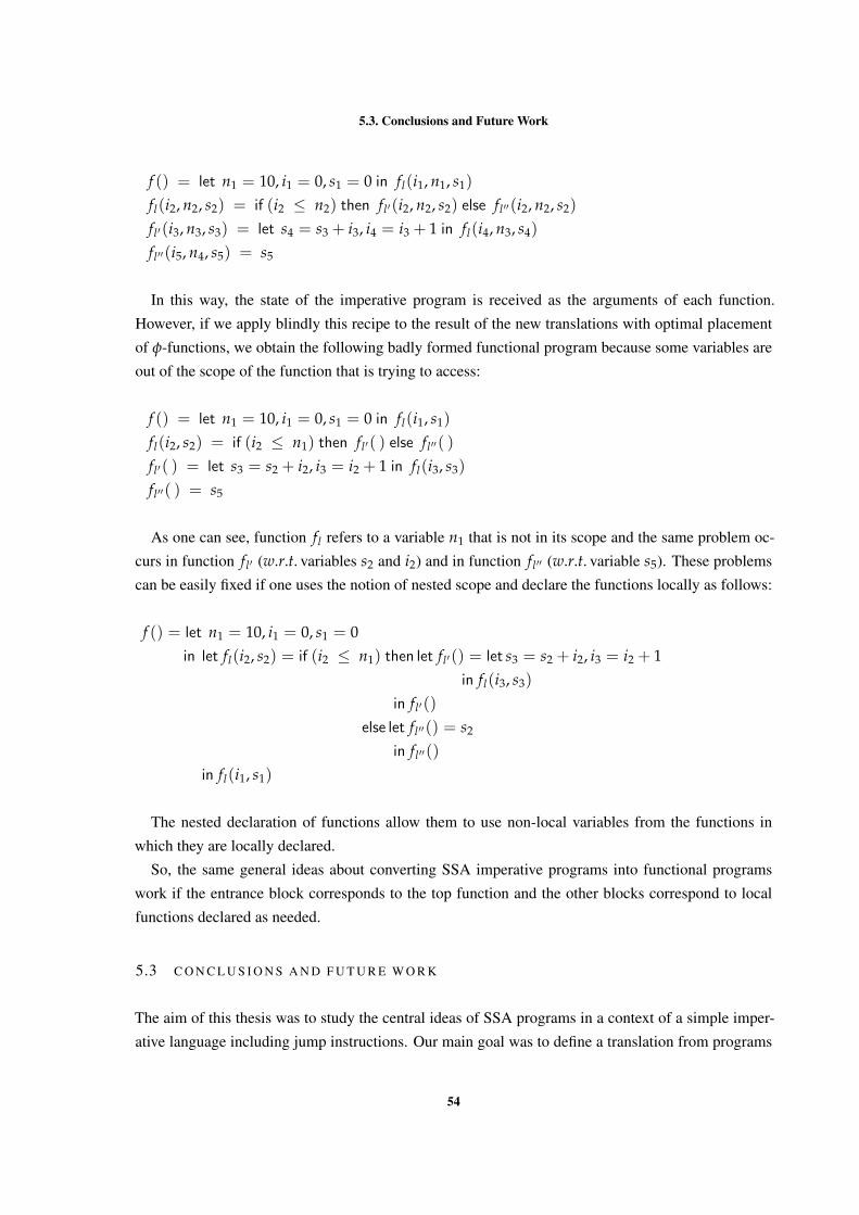
5.3. Conclusions and Future Work

....

f () = let n1 = 10, i1 = 0, s1 = 0 in fl(i1, n1, s1)

fl(i2, n2, s2) = if (i2 ≤ n2) then fl′(i2, n2, s2) else fl′′(i2, n2, s2)

fl′(i3, n3, s3) = let s4 = s3 + i3, i4 = i3 + 1 in fl(i4, n3, s4)

fl′′(i5, n4, s5) = s5

In this way, the state of the imperative program is received as the arguments of each function.

However, if we apply blindly this recipe to the result of the new translations with optimal placement

of φ-functions, we obtain the following badly formed functional program because some variables are

out of the scope of the function that is trying to access:

....

f () = let n1 = 10, i1 = 0, s1 = 0 in fl(i1, s1)

fl(i2, s2) = if (i2 ≤ n1) then fl′( ) else fl′′( )

fl′( ) = let s3 = s2 + i2, i3 = i2 + 1 in fl(i3, s3)

fl′′( ) = s5

As one can see, function fl refers to a variable n1 that is not in its scope and the same problem oc-

curs in function fl′ (w.r.t. variables s2 and i2) and in function fl′′ (w.r.t. variable s5). These problems

can be easily fixed if one uses the notion of nested scope and declare the functions locally as follows:

....

f () = let n1 = 10, i1 = 0, s1 = 0in let fl(i2, s2) = if (i2 ≤ n1) then let fl′() = let s3 = s2 + i2, i3 = i2 + 1

in fl(i3, s3)

in fl′()

else let fl′′() = s2

in fl′′()

in fl(i1, s1)

The nested declaration of functions allow them to use non-local variables from the functions in

which they are locally declared.

So, the same general ideas about converting SSA imperative programs into functional programs

work if the entrance block corresponds to the top function and the other blocks correspond to local

functions declared as needed.

5.3 C O N C L U S I O N S A N D F U T U R E W O R K

The aim of this thesis was to study the central ideas of SSA programs in a context of a simple imper-

ative language including jump instructions. Our main goal was to define a translation from programs

54

5.3. Conclusions and Future Work

of the base imperative language into the SSA format and to prove the correctness of the translation

process. We think this goal was successfully attained.

We chose to work in a setting of a very simple imperative language in order to focus our attention

in the essential and learn from it for future work. Even so, the task of proving correctness of SSA

translation was very demanding both on technical aspects and size. We have done this at a detailed

level but still there were some aspects treated informally. If on one hand it would have been extremely

helpful to have a proof assistant tool to deal with the complexity of size of our proof, on the other hand

the effort of formalizing our proof should require quite some time and this would be out of scope of this

work. Note, however, that the effort of addressing formal verification of SSA intermediate languages

has been considered in Barthe et al. (2012). This is a far more ambitious work, where in particular

translation from the source language RTL(Register Transfer Language) into SSA is addressed. The

language RTL is used in the formally verified compiler CompCert Leroy (2009) as a first step of

compilation of a realistic subset of the C programming language (prior to the compilation of RTL

into SSA). This overall framework is highly complex, and this makes very hard to understand in this

context the essential ideas for the correct translation into SSA of a source language with jumps.

The proof of correctness of the translation process has put several challenges regarding the def-

inition of the semantics both of source and SSA language and their interrelationship. After some

preliminary analysis it was clear for us that we would have to deal with small-step operational se-

mantics and that we needed to capture that the translation preserves semantics of the program in the

following sense: the CFG structure of the source code must be preserved and the state transformation

inside the blocks must be maintained to adequate versions of the variables. We highlight two key

ideas that have been essential to work around this issue: the isolation of the computation inside the

blocks and computation between blocks of code; and the introduction of a transition relation that does

the bookkeeping of the versions in use. So, we defined an alternative operational semantics, both

for the base imperative language and for the SSA language, which split the computation, according

to whether it involves a jump or not, and keeps track of information about the variables in order to

identify the adequate version of each variable, when relating execution of a base program and of its

SSA translation.

Regarding directions for future work, a task for the immediate future would be the correctness proof

of the new version of the translation function presented in Section 5.1. We think that this could be

done by adapting the proof we have developed in this thesis. Another line of work could be in the

context of the relation between SSA imperative programs and CPS functional programs.

In CPS each procedure takes an extra argument, its continuation, representing what should be done

with the result the function is calculating. Moreover, every argument in a function call must be either a

variable or the continuation. Adapting the example of Section 5.2 to CPS we would have the following

(by convention the continuation function is represented as a parameter named k)

55

5.3. Conclusions and Future Work

....

f (k) = let n1 = 10, i1 = 0, s1 = 0in let fl(i2, s2, k) = if (i2 ≤ n1) then let fl′(k) = let s3 = s2 + i2, i3 = i2 + 1

in fl(i3, s3, k)in fl′(k)

else let fl′′(k) = k s2

in fl′′(k)in fl(i1, s1, k)

A possible direction for future work is to study the central ideas about the CPS functional programs

and their relations with the SSA programs. Mutually inverse translation between CPS and SSA are

studied in Ferreira (2014) in a context where the programs only allow the SSA command assignment

and conditional. They build between them a syntactic bijection (at code level) and a semantic bijection

(at program execution level). We could profit from these ideas and apply them to a significantly richer

context where jump commands and recursion functions are present.

56

B I B L I O G R A P H Y

Andrew W. Appel. SSA is functional programming. SIGPLAN notices, 33(4):17–20, 1998a.

Andrew W. Appel. Modern Compiler Implementation in {C,Java,ML}. Cambridge University Press,

1998b.

Andrew W Appel. Compiling with continuations. Cambridge University Press, 2007.

Gilles Barthe, Delphine Demange, and David Pichardie. A formally verified SSA-based middle-end.

pages 47–66, 2012.

Alonzo Church. A set of postulates for the foundation of logic. Annals of mathematics, pages 346–366,

1932.

Ron Cytron, Jeanne Ferrante, Barry K Rosen, Mark N Wegman, and F Kenneth Zadeck. Efficiently

computing static single assignment form and the control dependence graph. ACM Transactions on

Programming Languages and Systems (TOPLAS), 13(4):451–490, 1991.

Tiago Alexandre da Costa Ferreira. Um estudo sobre a correspondencia entre programacao funcional

com continuacoes e programacao imperativa single assignment. Master’s thesis, Universidade do

Minho, Braga, 2014.

Richard A Kelsey. A correspondence between continuation passing style and static single assignment

form. In ACM SIGPLAN Notices, volume 30, pages 13–22. ACM, 1995.

Chris Lattner and Vikram Adve. Llvm: A compilation framework for lifelong program analysis &

transformation. In Code Generation and Optimization, 2004. CGO 2004. International Symposium

on, pages 75–86. IEEE, 2004.

Xavier Leroy. A formally verified compiler back-end. Journal of Automated Reasoning, 43(4):363–

446, 2009. URL http://gallium.inria.fr/˜xleroy/publi/compcert-backend.

pdf.

Steven S. Muchnick. Advanced Compiler Design and Implementation. Morgan Kaufmann, 1997a.

Steven S. Muchnick. Advanced compiler design implementation. Morgan Kaufmann, 1997b.

Richard Stallman. Using and porting the gnu compiler collection. In MIT Artificial Intelligence

Laboratory. Citeseer, 2001.

Michael Joseph Wolfe. High performance compilers for parallel computing. Addison-Wesley, 1996.

57

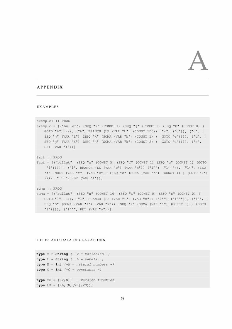
AA P P E N D I X

E X A M P L E S

exemple1 :: PROG

exemplo = [("bullet", (SEQ "i" (CONST 1) (SEQ "j" (CONST 1) (SEQ "k" (CONST 0) (

GOTO "b"))))), ("b", BRANCH (LE (VAR "k") (CONST 100)) ("c") ("d")), ("c", (

SEQ "j" (VAR "i") (SEQ "k" (SOMA (VAR "k") (CONST 1) ) (GOTO "e")))), ("d", (

SEQ "j" (VAR "k") (SEQ "k" (SOMA (VAR "k") (CONST 2) ) (GOTO "e")))), ("e",

RET (VAR "k"))]

fact :: PROG

fact = [("bullet", (SEQ "x" (CONST 5) (SEQ "f" (CONST 1) (SEQ "c" (CONST 1) (GOTO

"l"))))), ("l", BRANCH (LE (VAR "c") (VAR "x")) ("l’") ("l’’")), ("l’", (SEQ

"f" (MULT (VAR "f") (VAR "c")) (SEQ "c" (SOMA (VAR "c") (CONST 1) ) (GOTO "l")

))), ("l’’", RET (VAR "f"))]

suma :: PROG

suma = [("bullet", (SEQ "n" (CONST 10) (SEQ "i" (CONST 0) (SEQ "s" (CONST 0) (

GOTO "l"))))), ("l", BRANCH (LE (VAR "i") (VAR "n")) ("l’") ("l’’")), ("l’", (

SEQ "s" (SOMA (VAR "s") (VAR "i")) (SEQ "i" (SOMA (VAR "i") (CONST 1) ) (GOTO

"l")))), ("l’’", RET (VAR "s"))]

T Y P E S A N D DATA D E C L A R AT I O N S

type V = String {- V = variables -}

type L = String {- L = Labels -}

type N = Int {-N = natural numbers -}

type C = Int {-C = constants -}

type VS = [(V,N)] -- version function

type LS = [(L,(N,[VS],VS))]

58

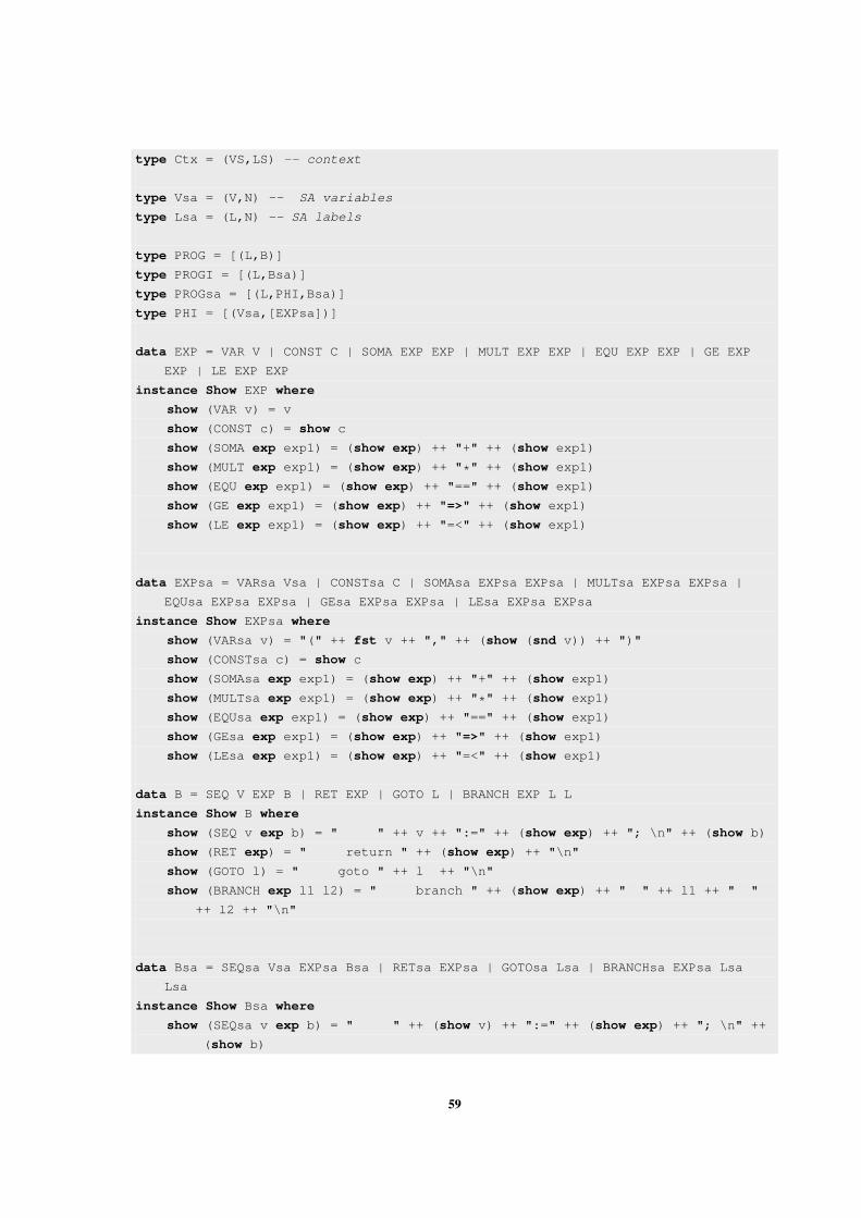
type Ctx = (VS,LS) -- context

type Vsa = (V,N) -- SA variables

type Lsa = (L,N) -- SA labels

type PROG = [(L,B)]

type PROGI = [(L,Bsa)]

type PROGsa = [(L,PHI,Bsa)]

type PHI = [(Vsa,[EXPsa])]

data EXP = VAR V | CONST C | SOMA EXP EXP | MULT EXP EXP | EQU EXP EXP | GE EXP

EXP | LE EXP EXP

instance Show EXP where

show (VAR v) = v

show (CONST c) = show c

show (SOMA exp exp1) = (show exp) ++ "+" ++ (show exp1)

show (MULT exp exp1) = (show exp) ++ "*" ++ (show exp1)

show (EQU exp exp1) = (show exp) ++ "==" ++ (show exp1)

show (GE exp exp1) = (show exp) ++ "=>" ++ (show exp1)

show (LE exp exp1) = (show exp) ++ "=<" ++ (show exp1)

data EXPsa = VARsa Vsa | CONSTsa C | SOMAsa EXPsa EXPsa | MULTsa EXPsa EXPsa |

EQUsa EXPsa EXPsa | GEsa EXPsa EXPsa | LEsa EXPsa EXPsa

instance Show EXPsa where

show (VARsa v) = "(" ++ fst v ++ "," ++ (show (snd v)) ++ ")"

show (CONSTsa c) = show c

show (SOMAsa exp exp1) = (show exp) ++ "+" ++ (show exp1)

show (MULTsa exp exp1) = (show exp) ++ "*" ++ (show exp1)

show (EQUsa exp exp1) = (show exp) ++ "==" ++ (show exp1)

show (GEsa exp exp1) = (show exp) ++ "=>" ++ (show exp1)

show (LEsa exp exp1) = (show exp) ++ "=<" ++ (show exp1)

data B = SEQ V EXP B | RET EXP | GOTO L | BRANCH EXP L L

instance Show B where

show (SEQ v exp b) = " " ++ v ++ ":=" ++ (show exp) ++ "; \n" ++ (show b)

show (RET exp) = " return " ++ (show exp) ++ "\n"

show (GOTO l) = " goto " ++ l ++ "\n"

show (BRANCH exp l1 l2) = " branch " ++ (show exp) ++ " " ++ l1 ++ " "

++ l2 ++ "\n"

data Bsa = SEQsa Vsa EXPsa Bsa | RETsa EXPsa | GOTOsa Lsa | BRANCHsa EXPsa Lsa

Lsa

instance Show Bsa where

show (SEQsa v exp b) = " " ++ (show v) ++ ":=" ++ (show exp) ++ "; \n" ++

(show b)

59

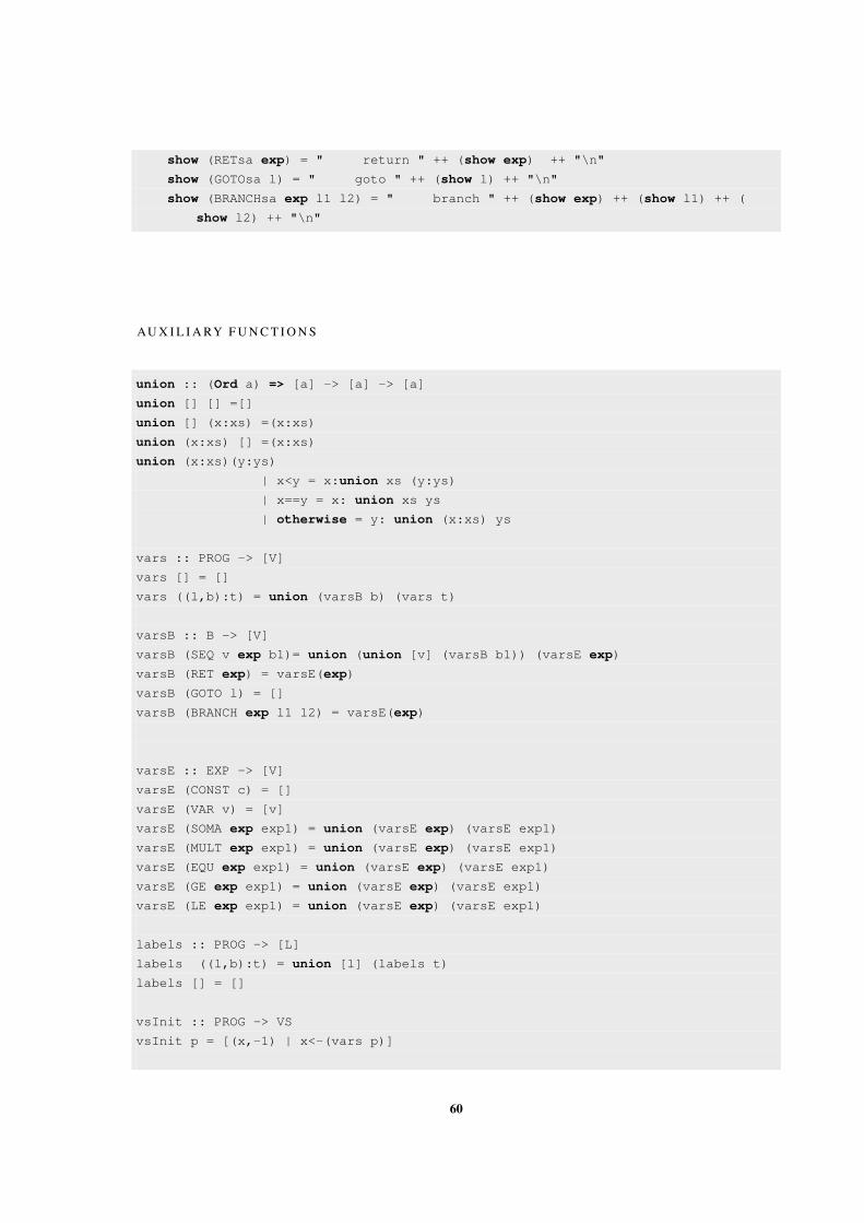
show (RETsa exp) = " return " ++ (show exp) ++ "\n"

show (GOTOsa l) = " goto " ++ (show l) ++ "\n"

show (BRANCHsa exp l1 l2) = " branch " ++ (show exp) ++ (show l1) ++ (

show l2) ++ "\n"

AU X I L I A RY F U N C T I O N S

union :: (Ord a) => [a] -> [a] -> [a]

union [] [] =[]

union [] (x:xs) =(x:xs)

union (x:xs) [] =(x:xs)

union (x:xs)(y:ys)

| x<y = x:union xs (y:ys)

| x==y = x: union xs ys

| otherwise = y: union (x:xs) ys

vars :: PROG -> [V]

vars [] = []

vars ((l,b):t) = union (varsB b) (vars t)

varsB :: B -> [V]

varsB (SEQ v exp b1)= union (union [v] (varsB b1)) (varsE exp)

varsB (RET exp) = varsE(exp)

varsB (GOTO l) = []

varsB (BRANCH exp l1 l2) = varsE(exp)

varsE :: EXP -> [V]

varsE (CONST c) = []

varsE (VAR v) = [v]

varsE (SOMA exp exp1) = union (varsE exp) (varsE exp1)

varsE (MULT exp exp1) = union (varsE exp) (varsE exp1)

varsE (EQU exp exp1) = union (varsE exp) (varsE exp1)

varsE (GE exp exp1) = union (varsE exp) (varsE exp1)

varsE (LE exp exp1) = union (varsE exp) (varsE exp1)

labels :: PROG -> [L]

labels ((l,b):t) = union [l] (labels t)

labels [] = []

vsInit :: PROG -> VS

vsInit p = [(x,-1) | x<-(vars p)]

60

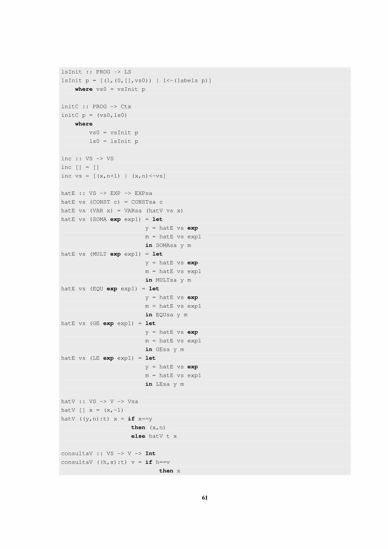
lsInit :: PROG -> LS

lsInit p = [(l,(0,[],vs0)) | l<-(labels p)]

where vs0 = vsInit p

initC :: PROG -> Ctx

initC p = (vs0,ls0)

where

vs0 = vsInit p

ls0 = lsInit p

inc :: VS -> VS

inc [] = []

inc vs = [(x,n+1) | (x,n)<-vs]

hatE :: VS -> EXP -> EXPsa

hatE vs (CONST c) = CONSTsa c

hatE vs (VAR x) = VARsa (hatV vs x)

hatE vs (SOMA exp exp1) = let

y = hatE vs exp

m = hatE vs exp1

in SOMAsa y m

hatE vs (MULT exp exp1) = let

y = hatE vs exp

m = hatE vs exp1

in MULTsa y m

hatE vs (EQU exp exp1) = let

y = hatE vs exp

m = hatE vs exp1

in EQUsa y m

hatE vs (GE exp exp1) = let

y = hatE vs exp

m = hatE vs exp1

in GEsa y m

hatE vs (LE exp exp1) = let

y = hatE vs exp

m = hatE vs exp1

in LEsa y m

hatV :: VS -> V -> Vsa

hatV [] x = (x,-1)

hatV ((y,n):t) x = if x==y

then (x,n)

else hatV t x

consultaV :: VS -> V -> Int

consultaV ((h,x):t) v = if h==v

then x

61

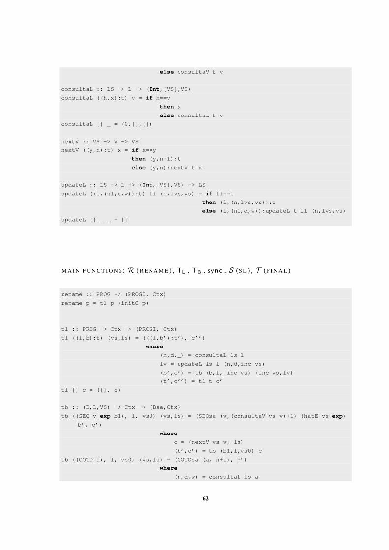
else consultaV t v

consultaL :: LS -> L -> (Int,[VS],VS)

consultaL ((h,x):t) v = if h==v

then x

else consultaL t v

consultaL [] _ = (0,[],[])

nextV :: VS -> V -> VS

nextV ((y,n):t) x = if x==y

then (y,n+1):t

else (y,n):nextV t x

updateL :: LS -> L -> (Int,[VS],VS) -> LS

updateL ((l,(n1,d,w)):t) l1 (n,lvs,vs) = if l1==l

then (l,(n,lvs,vs)):t

else (l,(n1,d,w)):updateL t l1 (n,lvs,vs)

updateL [] _ _ = []

M A I N F U N C T I O N S : R ( R E N A M E ) , TL , TB , sync , S ( S L ) , T ( F I N A L )

rename :: PROG -> (PROGI, Ctx)

rename p = tl p (initC p)

tl :: PROG -> Ctx -> (PROGI, Ctx)

tl ((l,b):t) (vs,ls) = (((l,b’):t’), c’’)

where

(n,d,_) = consultaL ls l

lv = updateL ls l (n,d,inc vs)

(b’,c’) = tb (b,l, inc vs) (inc vs,lv)

(t’,c’’) = tl t c’

tl [] c = ([], c)

tb :: (B,L,VS) -> Ctx -> (Bsa,Ctx)

tb ((SEQ v exp b1), l, vs0) (vs,ls) = (SEQsa (v,(consultaV vs v)+1) (hatE vs exp)

b’, c’)

where

c = (nextV vs v, ls)

(b’,c’) = tb (b1,l,vs0) c

tb ((GOTO a), l, vs0) (vs,ls) = (GOTOsa (a, n+1), c’)

where

(n,d,w) = consultaL ls a

62

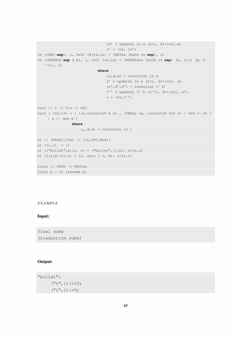
ls’ = updateL ls a (n+1, d++[vs],w)

c’ = (vs, ls’)

tb ((RET exp), l, vs0) c@(vs,ls) = (RETsa (hatE vs exp), c)

tb ((BRANCH exp a b), l, vs0) (vs,ls) = (BRANCHsa (hatE vs exp) (a, n+1) (b, n

’+1), c)

where

(n,d,w) = consultaL ls a

l’ = updateL ls a (n+1, d++[vs], w)

(n’,d’,w’) = consultaL l’ b

l’’ = updateL l’ b (n’+1, d++[vs], w’)

c = (vs,l’’)

sync :: L -> Ctx -> PHI

sync l (vs,ls) = [ ((x,consultaV w x) , [VARsa (x, consultaV vs0 x) | vs0 <- d] )

| x <- dom w ]

where

(_,d,w) = consultaL ls l

sl :: (PROGI,Ctx) -> [(L,PHI,Bsa)]

sl ([],c) = []

sl (("bullet",b):t, c) = ("bullet",[],b): sl(t,c)

sl (((l,b):t),c) = (l, sync l c, b): sl(t,c)

final :: PROG -> PROGsa

final p = sl (rename p)

E X A M P L E

Input:

final suma

(traduction suma)

Output:

"bullet":

("n",1):=10;

("i",1):=0;

63

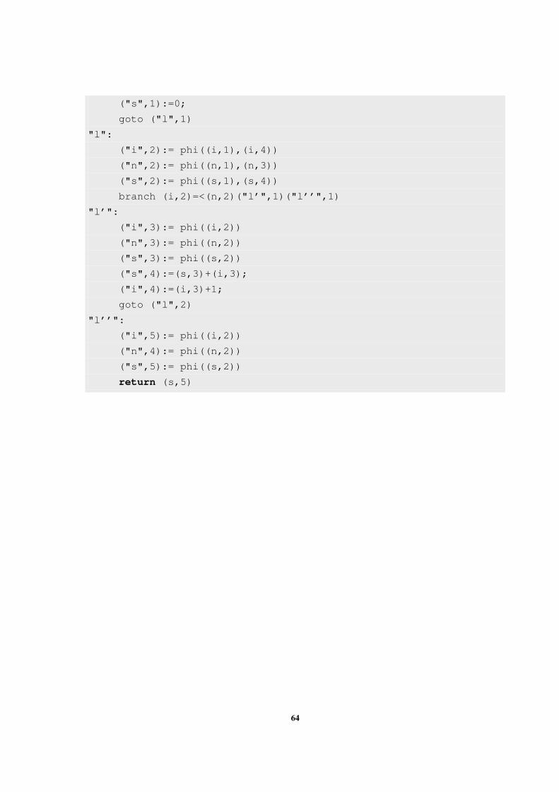
("s",1):=0;

goto ("l",1)

"l":

("i",2):= phi((i,1),(i,4))

("n",2):= phi((n,1),(n,3))

("s",2):= phi((s,1),(s,4))

branch (i,2)=<(n,2)("l’",1)("l’’",1)

"l’":

("i",3):= phi((i,2))

("n",3):= phi((n,2))

("s",3):= phi((s,2))

("s",4):=(s,3)+(i,3);

("i",4):=(i,3)+1;

goto ("l",2)

"l’’":

("i",5):= phi((i,2))

("n",4):= phi((n,2))

("s",5):= phi((s,2))

return (s,5)

64

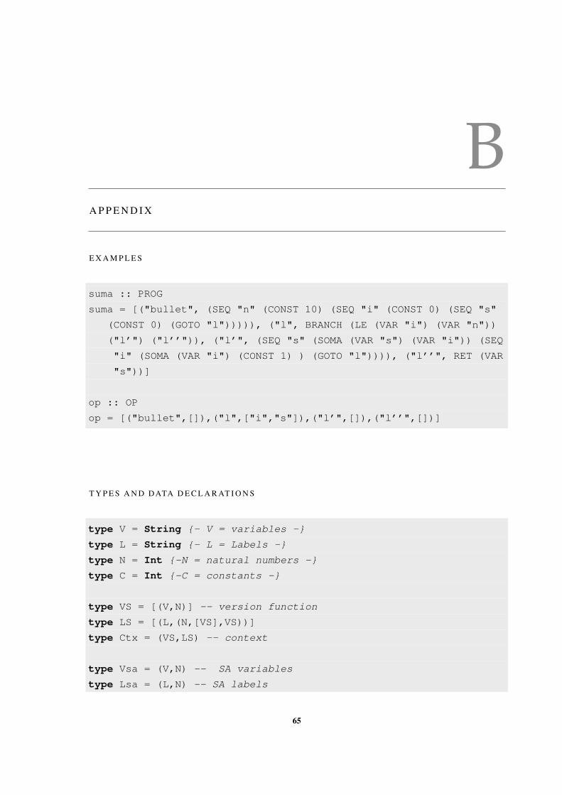
BA P P E N D I X

E X A M P L E S

suma :: PROG

suma = [("bullet", (SEQ "n" (CONST 10) (SEQ "i" (CONST 0) (SEQ "s"

(CONST 0) (GOTO "l"))))), ("l", BRANCH (LE (VAR "i") (VAR "n"))

("l’") ("l’’")), ("l’", (SEQ "s" (SOMA (VAR "s") (VAR "i")) (SEQ

"i" (SOMA (VAR "i") (CONST 1) ) (GOTO "l")))), ("l’’", RET (VAR

"s"))]

op :: OP

op = [("bullet",[]),("l",["i","s"]),("l’",[]),("l’’",[])]

T Y P E S A N D DATA D E C L A R AT I O N S

type V = String {- V = variables -}

type L = String {- L = Labels -}

type N = Int {-N = natural numbers -}

type C = Int {-C = constants -}

type VS = [(V,N)] -- version function

type LS = [(L,(N,[VS],VS))]

type Ctx = (VS,LS) -- context

type Vsa = (V,N) -- SA variables

type Lsa = (L,N) -- SA labels

65

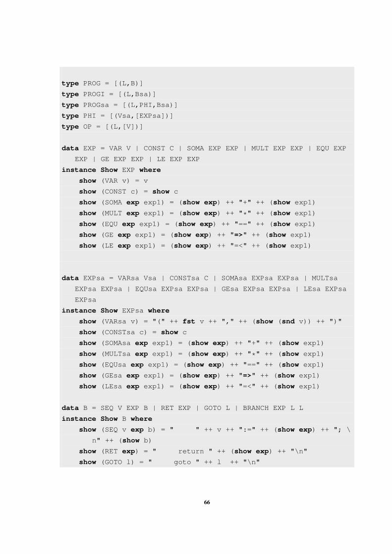
type PROG = [(L,B)]

type PROGI = [(L,Bsa)]

type PROGsa = [(L,PHI,Bsa)]

type PHI = [(Vsa,[EXPsa])]

type OP = [(L,[V])]

data EXP = VAR V | CONST C | SOMA EXP EXP | MULT EXP EXP | EQU EXP

EXP | GE EXP EXP | LE EXP EXP

instance Show EXP where

show (VAR v) = v

show (CONST c) = show c

show (SOMA exp exp1) = (show exp) ++ "+" ++ (show exp1)

show (MULT exp exp1) = (show exp) ++ "*" ++ (show exp1)

show (EQU exp exp1) = (show exp) ++ "==" ++ (show exp1)

show (GE exp exp1) = (show exp) ++ "=>" ++ (show exp1)

show (LE exp exp1) = (show exp) ++ "=<" ++ (show exp1)

data EXPsa = VARsa Vsa | CONSTsa C | SOMAsa EXPsa EXPsa | MULTsa

EXPsa EXPsa | EQUsa EXPsa EXPsa | GEsa EXPsa EXPsa | LEsa EXPsa

EXPsa

instance Show EXPsa where

show (VARsa v) = "(" ++ fst v ++ "," ++ (show (snd v)) ++ ")"

show (CONSTsa c) = show c

show (SOMAsa exp exp1) = (show exp) ++ "+" ++ (show exp1)

show (MULTsa exp exp1) = (show exp) ++ "*" ++ (show exp1)

show (EQUsa exp exp1) = (show exp) ++ "==" ++ (show exp1)

show (GEsa exp exp1) = (show exp) ++ "=>" ++ (show exp1)

show (LEsa exp exp1) = (show exp) ++ "=<" ++ (show exp1)

data B = SEQ V EXP B | RET EXP | GOTO L | BRANCH EXP L L

instance Show B where

show (SEQ v exp b) = " " ++ v ++ ":=" ++ (show exp) ++ "; \

n" ++ (show b)

show (RET exp) = " return " ++ (show exp) ++ "\n"

show (GOTO l) = " goto " ++ l ++ "\n"

66

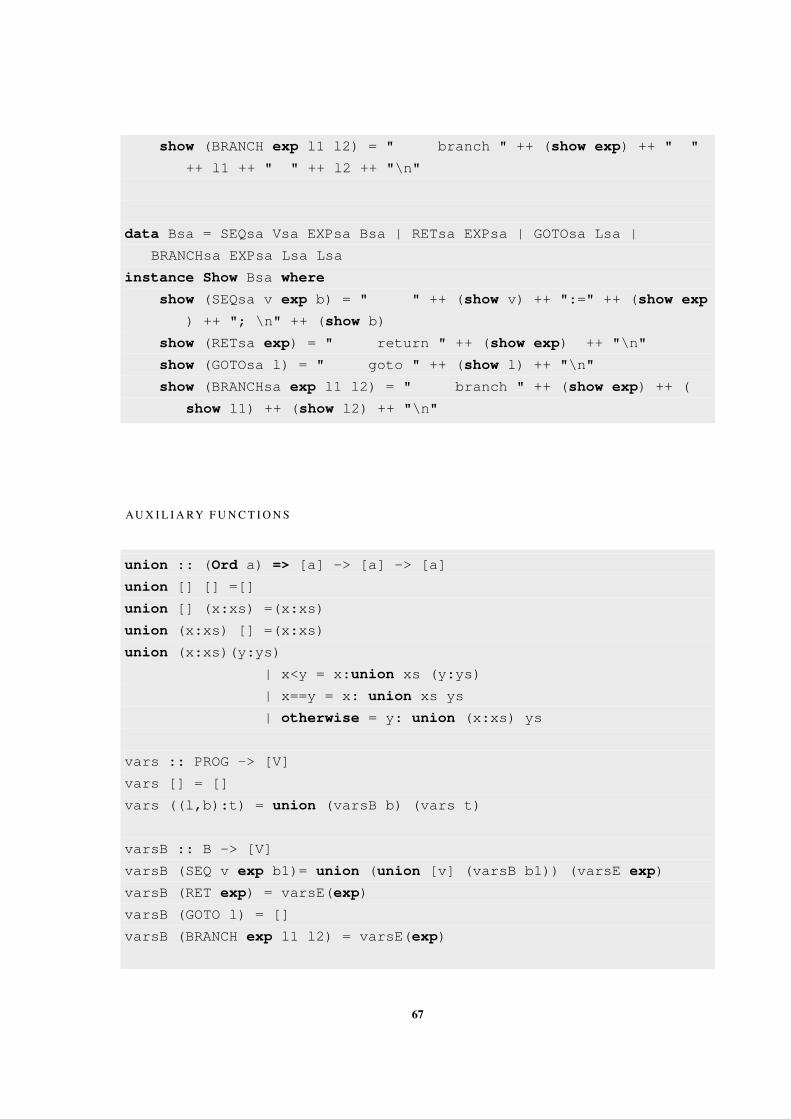
show (BRANCH exp l1 l2) = " branch " ++ (show exp) ++ " "

++ l1 ++ " " ++ l2 ++ "\n"

data Bsa = SEQsa Vsa EXPsa Bsa | RETsa EXPsa | GOTOsa Lsa |

BRANCHsa EXPsa Lsa Lsa

instance Show Bsa where

show (SEQsa v exp b) = " " ++ (show v) ++ ":=" ++ (show exp

) ++ "; \n" ++ (show b)

show (RETsa exp) = " return " ++ (show exp) ++ "\n"

show (GOTOsa l) = " goto " ++ (show l) ++ "\n"

show (BRANCHsa exp l1 l2) = " branch " ++ (show exp) ++ (

show l1) ++ (show l2) ++ "\n"

AU X I L I A RY F U N C T I O N S

union :: (Ord a) => [a] -> [a] -> [a]

union [] [] =[]

union [] (x:xs) =(x:xs)

union (x:xs) [] =(x:xs)

union (x:xs)(y:ys)

| x<y = x:union xs (y:ys)

| x==y = x: union xs ys

| otherwise = y: union (x:xs) ys

vars :: PROG -> [V]

vars [] = []

vars ((l,b):t) = union (varsB b) (vars t)

varsB :: B -> [V]

varsB (SEQ v exp b1)= union (union [v] (varsB b1)) (varsE exp)

varsB (RET exp) = varsE(exp)

varsB (GOTO l) = []

varsB (BRANCH exp l1 l2) = varsE(exp)

67

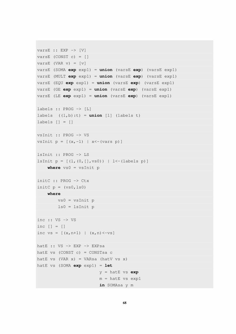
varsE :: EXP -> [V]

varsE (CONST c) = []

varsE (VAR v) = [v]

varsE (SOMA exp exp1) = union (varsE exp) (varsE exp1)

varsE (MULT exp exp1) = union (varsE exp) (varsE exp1)

varsE (EQU exp exp1) = union (varsE exp) (varsE exp1)

varsE (GE exp exp1) = union (varsE exp) (varsE exp1)

varsE (LE exp exp1) = union (varsE exp) (varsE exp1)

labels :: PROG -> [L]

labels ((l,b):t) = union [l] (labels t)

labels [] = []

vsInit :: PROG -> VS

vsInit p = [(x,-1) | x<-(vars p)]

lsInit :: PROG -> LS

lsInit p = [(l,(0,[],vs0)) | l<-(labels p)]

where vs0 = vsInit p

initC :: PROG -> Ctx

initC p = (vs0,ls0)

where

vs0 = vsInit p

ls0 = lsInit p

inc :: VS -> VS

inc [] = []

inc vs = [(x,n+1) | (x,n)<-vs]

hatE :: VS -> EXP -> EXPsa

hatE vs (CONST c) = CONSTsa c

hatE vs (VAR x) = VARsa (hatV vs x)

hatE vs (SOMA exp exp1) = let

y = hatE vs exp

m = hatE vs exp1

in SOMAsa y m

68

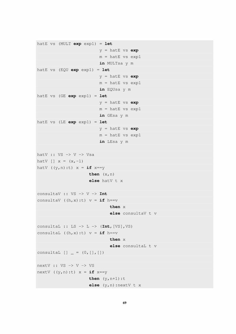
hatE vs (MULT exp exp1) = let

y = hatE vs exp

m = hatE vs exp1

in MULTsa y m

hatE vs (EQU exp exp1) = let

y = hatE vs exp

m = hatE vs exp1

in EQUsa y m

hatE vs (GE exp exp1) = let

y = hatE vs exp

m = hatE vs exp1

in GEsa y m

hatE vs (LE exp exp1) = let

y = hatE vs exp

m = hatE vs exp1

in LEsa y m

hatV :: VS -> V -> Vsa

hatV [] x = (x,-1)

hatV ((y,n):t) x = if x==y

then (x,n)

else hatV t x

consultaV :: VS -> V -> Int

consultaV ((h,x):t) v = if h==v

then x

else consultaV t v

consultaL :: LS -> L -> (Int,[VS],VS)

consultaL ((h,x):t) v = if h==v

then x

else consultaL t v

consultaL [] _ = (0,[],[])

nextV :: VS -> V -> VS

nextV ((y,n):t) x = if x==y

then (y,n+1):t

else (y,n):nextV t x

69

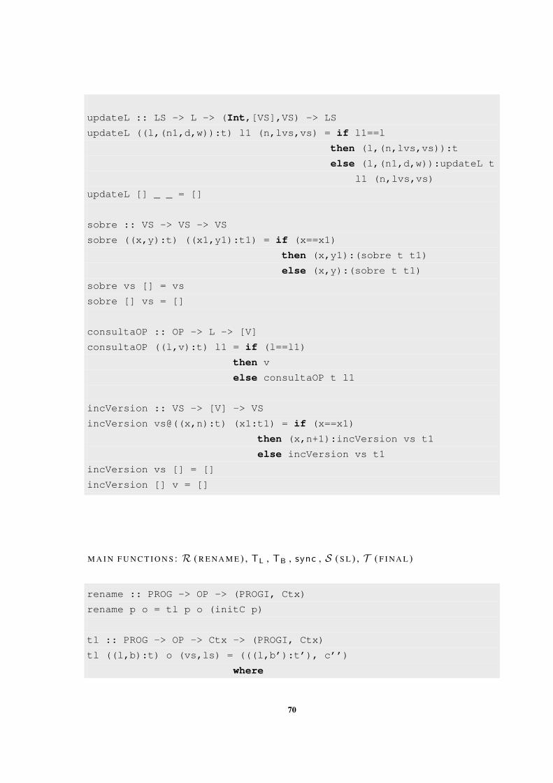
updateL :: LS -> L -> (Int,[VS],VS) -> LS

updateL ((l,(n1,d,w)):t) l1 (n,lvs,vs) = if l1==l

then (l,(n,lvs,vs)):t

else (l,(n1,d,w)):updateL t

l1 (n,lvs,vs)

updateL [] _ _ = []

sobre :: VS -> VS -> VS

sobre ((x,y):t) ((x1,y1):t1) = if (x==x1)

then (x,y1):(sobre t t1)

else (x,y):(sobre t t1)

sobre vs [] = vs

sobre [] vs = []

consultaOP :: OP -> L -> [V]

consultaOP ((l,v):t) l1 = if (l==l1)

then v

else consultaOP t l1

incVersion :: VS -> [V] -> VS

incVersion vs@((x,n):t) (x1:t1) = if (x==x1)

then (x,n+1):incVersion vs t1

else incVersion vs t1

incVersion vs [] = []

incVersion [] v = []

M A I N F U N C T I O N S : R ( R E N A M E ) , TL , TB , sync , S ( S L ) , T ( F I N A L )

rename :: PROG -> OP -> (PROGI, Ctx)

rename p o = tl p o (initC p)

tl :: PROG -> OP -> Ctx -> (PROGI, Ctx)

tl ((l,b):t) o (vs,ls) = (((l,b’):t’), c’’)

where

70

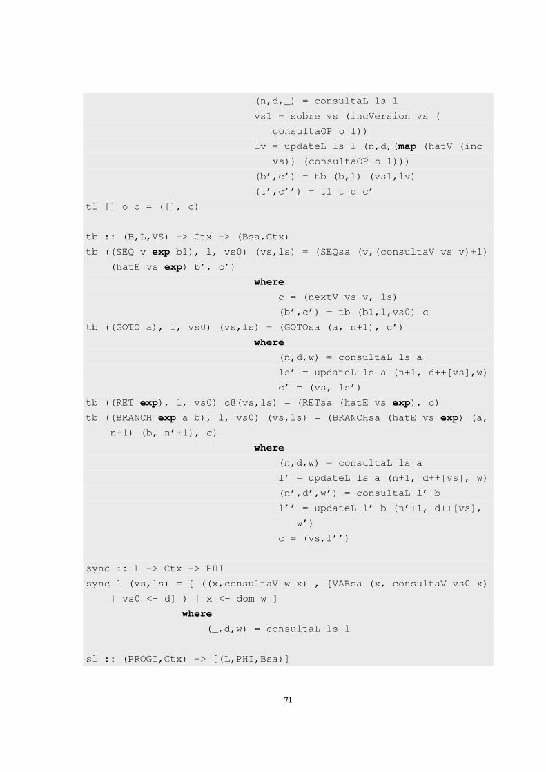
(n,d,_) = consultaL ls l

vs1 = sobre vs (incVersion vs (

consultaOP o l))

lv = updateL ls l (n,d,(map (hatV (inc

vs)) (consultaOP o l)))

(b’,c’) = tb (b,l) (vs1,lv)

(t’,c’’) = tl t o c’

tl [] o c = ([], c)

tb :: (B,L,VS) -> Ctx -> (Bsa,Ctx)

tb ((SEQ v exp b1), l, vs0) (vs,ls) = (SEQsa (v,(consultaV vs v)+1)

(hatE vs exp) b’, c’)

where

c = (nextV vs v, ls)

(b’,c’) = tb (b1,l,vs0) c

tb ((GOTO a), l, vs0) (vs,ls) = (GOTOsa (a, n+1), c’)

where

(n,d,w) = consultaL ls a

ls’ = updateL ls a (n+1, d++[vs],w)

c’ = (vs, ls’)

tb ((RET exp), l, vs0) c@(vs,ls) = (RETsa (hatE vs exp), c)

tb ((BRANCH exp a b), l, vs0) (vs,ls) = (BRANCHsa (hatE vs exp) (a,

n+1) (b, n’+1), c)

where

(n,d,w) = consultaL ls a

l’ = updateL ls a (n+1, d++[vs], w)

(n’,d’,w’) = consultaL l’ b

l’’ = updateL l’ b (n’+1, d++[vs],

w’)

c = (vs,l’’)

sync :: L -> Ctx -> PHI

sync l (vs,ls) = [ ((x,consultaV w x) , [VARsa (x, consultaV vs0 x)

| vs0 <- d] ) | x <- dom w ]

where

(_,d,w) = consultaL ls l

sl :: (PROGI,Ctx) -> [(L,PHI,Bsa)]

71

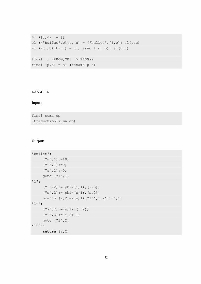
sl ([],c) = []

sl (("bullet",b):t, c) = ("bullet",[],b): sl(t,c)

sl (((l,b):t),c) = (l, sync l c, b): sl(t,c)

final :: (PROG,OP) -> PROGsa

final (p,o) = sl (rename p o)

E X A M P L E

Input:

final suma op

(traduction suma op)

Output:

"bullet":

("n",1):=10;

("i",1):=0;

("s",1):=0;

goto ("l",1)

"l":

("i",2):= phi((i,1),(i,3))

("s",2):= phi((s,1),(s,2))

branch (i,2)=<(n,1)("l’",1)("l’’",1)

"l’":

("s",2):=(s,1)+(i,2);

("i",3):=(i,2)+1;

goto ("l",2)

"l’’":

return (s,2)

72