ground truth determination for segmentation of tomographic ... · ground truth determination for...

Beatriz Leão Rodolpho

Licenciatura em Ciências de Engenharia Biomédica

Ground Truth Determination for Segmentation of Tomographic Volumes

Using Interpolation

Dissertação para obtenção do Grau de Mestre em Engenharia Biomédica

Adviser: Dr. Deidre Meldrum, The Biodesign Institute, ASU Co-advisers: Dr. Roger Johnson, The Biodesign Institute, ASU and Dr. Mário Secca, FCT-UNL

Júri: (Júri:

Presidente: Doutora Maria Adelaide de Almeida Pedro de Jesus,

FCT-UNL Arguente: Doutor André Teixeira Bento Damas Mora, FCT-UNL

Vogal: Doutor Mário António Basto Forjaz Secca, FCT-UNL

Outubro de 2013

Ground Truth Determination for Segmentation of Tomographic Volumes Using Interpolation Copyright©2013 – Todos os Direitos Reservados. Beatriz Leão Rodolpho, FCT/UNL e UNL A Faculdade de Ciências e Tecnologia e a Universidade Nova de Lisboa tem o direito, perpétuo e sem limites geográficos de arquivar e publicar esta dissertação através de exemplares impressos reproduzidos em papel ou de forma digital, ou por qualquer outro meio conhecido ou que venha a ser inventado, e de a divulgar através de repositórios científicos e de admitir a sua cópia e distribuição com objectivos educacionais ou de investigação, não comerciais, desde que seja dado crédito ao autor e editor.

v

“Consider it pure joy, my brothers and sisters, whenever you face trials of many

kinds, because you know that the testing of your faith produces perseverance. Let

perseverance finish its work so that you may be mature and complete, not lacking

anything” – James 1:2-4

vii

ACKNOWLEDGEMENTS

This work has benefited greatly from the input of several people. I would first

and foremost like to thank my advisor, Dr. Deidre Meldrum of the Center for

Biosignatures Discovery Automation (CBDA) at Arizona State University, who

deserves much credit for the overarching direction of this research and

insightful guidance. Thanks are due to Dr. Roger Johnson of Arizona State

University, for his support, guidance, and persistence along the duration of this

research. I would also like to thank my advisor at the Universidade Nova de

Lisboa, Dr. Mario Seca, for his willingness to oversee my studies in the United

States. The ability to conduct my research abroad significantly molded my

experience as a student and as a person; I would like to thank these three

people for their willingness to facilitate this arrangement.

Special thanks go to Dr. Brian Ashcroft of Arizona State University for his

profound impact on my research and for his day-to-day mentorship and

friendship in the lab. This research could not have been done without his help. I

would also like to thank Dr. Vivek Nandakumar for overseeing the research

project.

Completion of my thesis would not have been possible without the help of my

research colleagues and team members in the CBDA lab. These persons

included Stephanie Helland, Kathryn Hernandez, and Miranda Slaydon. I would

like to thank them for their insight and friendship throughout the thesis process.

A special thanks to Berit Kloster for her support throughout my college career.

I would like to thank my family, friends and college colleagues who—through

their patient and gracious sacrifice—have helped me to reach this goal. I would

like to especially thank my father and mother, Antonio and Maria Rodolpho, my

sisters, Natalia Bandeira and Letícia Rodolpho, and my boyfriend, Chuck Davis,

for their unwavering love and support.

Finally, I would like to thank God for giving me the capability and strength

necessary do conclude this research.

ix

ABSTRACT

Optical projection tomographic microscopy allows for a 3D analysis of individual

cells, making it possible to study its morphology. The 3D imagining technique

used in this thesis uses white light excitation to image stained cells, and is

referred to as single-cell optical computed tomography (cell CT).

Studies have shown that morphological characteristics of the cell and its

nucleus are deterministic in cancer diagnoses. For a more complete and

accurate analysis of these characteristics, a fully-automated analysis of the

single-cell 3D tomographic images can be done. The first step is segmenting

the image into the different cell components. To assess how accurate the

segmentation is, there is a need to determine ground truth of the automated

segmentation.

This dissertation intends to expose a method of obtaining ground truth for 3D

segmentation of single cells. This was achieved by developing a software in C-

Sharp. The software allows the user to input a visual segmentation of each 2D

slice of a 3D volume by using a pen to trace the visually identified boundary of a

cell component on a tablet. With this information, the software creates a

segmentation of a 3D tomographic image that is a result of human visual

segmentation.

To increase the speed of this process, interpolation algorithms can be used.

Since it is very time consuming to draw on every slice the user can skip slices.

Interpolation algorithms are used to interpolate on the skipped slices.

Five different interpolation algorithms were written: Linear Interpolation,

Gaussian splat, Marching Cubes, Unorganized Points, and Delaunay

Triangulation. To evaluate the performance of each interpolation algorithm the

following evaluation metrics were used: Jaccard Similarity, Dice Coefficient,

Specificity and Sensitivity.

x

After evaluating each interpolation method we concluded that linear

interpolation was the most accurate interpolation method, producing the best

segmented volume for a faster ground truth determination method.

Keywords: 3D segmentation, ground truth, computed tomography, cancer, 3D

interpolation, software

xi

RESUMO

A tomografia óptica microscópica de projecção permite uma análise 3D de

células individuais, tornando possível estudar a sua morfologia. A técnica de

imagiologia 3D utilizada nesta tese utiliza excitação por luz branca para obter

imagens de células pigmentadas, e é chamada de tomografia óptica

computadorizada celular (cell CT).

Estudos mostram que as características morfológicas da célula e do seu núcleo

são determinísticas no diagnóstico do cancro. Para uma análise mais complete

a precisa dessas características uma análise completamente automatizada

pode ser feita das imagens 3D celulares tomográficas. O primeiro passo é

segmentar a imagem nos diferentes componentes celulares. Para avaliar a

precisão da segmentação é necessário estabelecer ground truth, ou a verdade

absoluta, para a segmentação automatizada.

Esta dissertação pretende expor um método de obter ground truth para

segmentação 3D de células individuais. Isto foi conseguido através de um

software desenvolvido em C-Sharp. O software permite ao utilizador introduzir

a sua segmentação visual de cada fatia 2D de um volume 3D, utilizando uma

caneta para delinear o limite de um componente celular num tablet. Com esta

informação, o software cria a segmentação de uma imagem tomográfica 3D,

que é o resultado de uma segmentação visual humana.

Para aumentar a rapidez deste processo, algoritmos de interpolação podem ser

utilizados. Dado que é demorado desenhar em todas as fatias, o utilizador pode

saltar fatias. Algoritmos de interpolação são utilizados para interpolar nas fatias

que foram saltadas.

Cinco algoritmos diferentes foram estudados: Interpolação Linear, Kernel

Gaussiano, Cubos Marchantes, Pontos Desorganizados, e Triangulação de

Delaunay. Para avaliar o desempenho de cada algoritmo de interpolação as

seguintes métricas de avaliação foram utilizadas: Índice de Jaccard,

Coeficiente de Dice, Especificidade e Sensibilidade.

xii

Após avaliar cada método de interpolação concluímos que a Interpolação

Linear é o método de interpolação mais preciso, produzindo o melhor volume

segmentado para um método de obtenção de ground truth mais rápido.

Termos chave: segmentação 3D, ground truth, tomográfica computorizada,

cancro, interpolação 3D, software

xiii

Table of Contents Acknowledgements ........................................................................................... vii

Abstract .............................................................................................................. ix

Resumo .............................................................................................................. xi

List of Figures .................................................................................................... xv

List of Tables ................................................................................................... xvii

List of Abbreviations and Acronyms ................................................................. xix

1. Introduction ................................................................................................. 1

1.1 Motivation .............................................................................................. 1

1.2 Research Goal ...................................................................................... 3

1.3 Optical Cell – CT ................................................................................... 4

1.3.1 The cell CT Instrument ................................................................... 4

1.3.2 Projection Image Acquisition .......................................................... 5

1.4 Segmentation Algorithms ...................................................................... 6

1.4.1 Rosin’s threshold method ................................................................... 6

1.4.2 Otsu’s method .................................................................................... 7

1.4.3 K-means Clustering ............................................................................ 9

1.5 State of the Art .................................................................................... 10

2. Methods .................................................................................................... 13

2.1 Cell Sample Preparation ..................................................................... 13

2.2 Ground Truth Evaluation Software ...................................................... 14

2.3 Interpolation Algorithms ....................................................................... 22

2.2.1 Linear Interpolation ........................................................................... 22

2.2.2 Marching Cubes ............................................................................... 24

xiv

2.2.3 Gaussian Splat ................................................................................. 27

2.2.4 Delaunay Triangulation .................................................................... 28

2.2.5 Unorganized Points .......................................................................... 31

2.4 Evaluation Metrics ............................................................................... 32

2.4.1 Jaccard Similarity .......................................................................... 34

2.4.2 Dice’s Coefficient .......................................................................... 35

2.4.3 Specificity ..................................................................................... 35

2.4.4 Sensitivity ..................................................................................... 36

3. Results ...................................................................................................... 37

3.1 Inter–user variance.............................................................................. 37

3.2 Interpolated Volumes .......................................................................... 38

3.2.1 Linear Interpolation ....................................................................... 38

3.2.2 Marching Cubes ............................................................................ 40

3.2.3 Gaussian Splat ............................................................................. 41

3.2.4 Delaunay Triangulation ................................................................. 42

3.2.5 Unorganized Points ...................................................................... 43

4. Discussion ................................................................................................. 47

4.1 Software’s Inter-user variability ........................................................... 47

4.2 Interpolation Algorithms ....................................................................... 47

5. Conclusion ................................................................................................ 55

Bibliography ...................................................................................................... 57

Appendix A: Pseudo code for the Linear Interpolation and Marching Cubes

algorithms ......................................................................................................... 61

xv

LIST OF FIGURES

Figure 1.1 - 3D image of a cancer cell generated by the cell CT. Artificial color

was added to the nucleus and its components. .................................................. 2

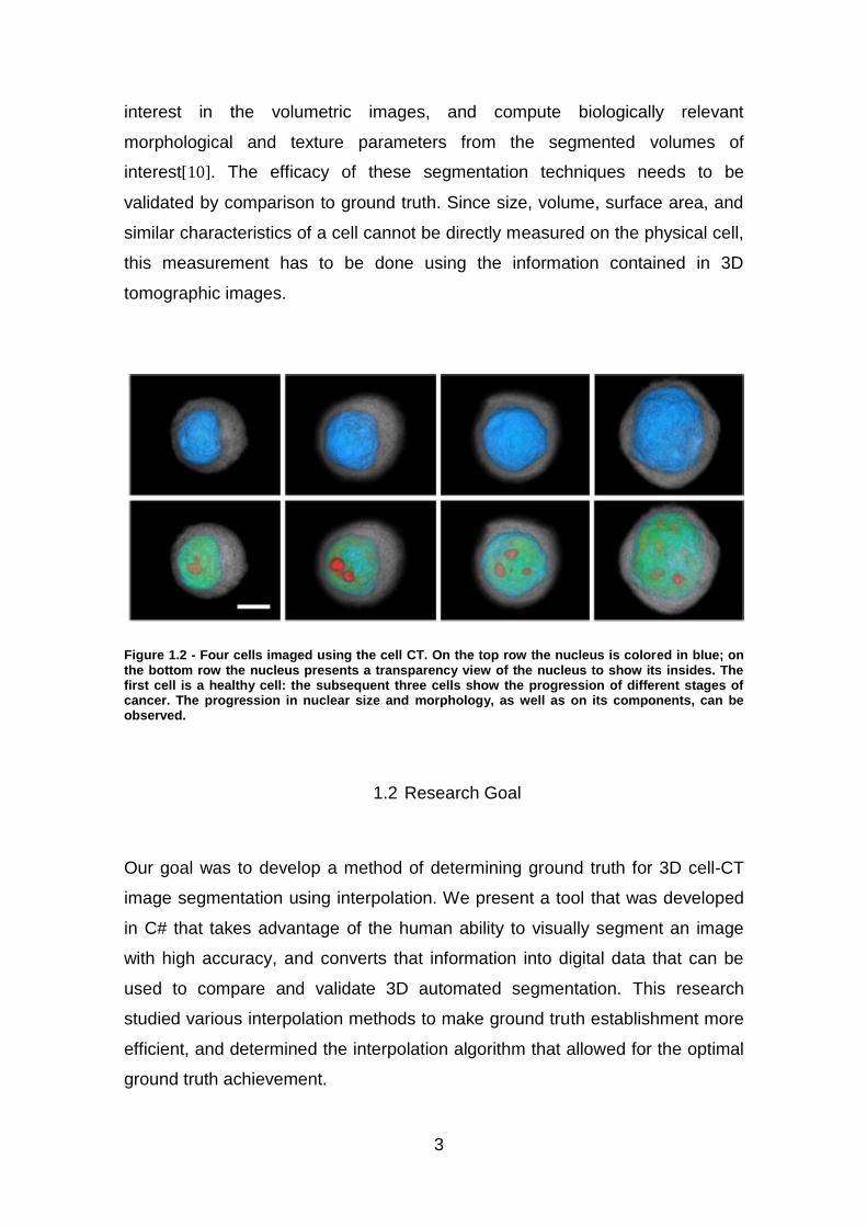
Figure 1.2 - Four cells imaged using the cell CT. On the top row the nucleus is

colored in blue; on the bottom row the nucleus presents a transparency view of

the nucleus to show its insides. The first cell is a healthy cell: the subsequent

three cells show the progression of different stages of cancer. The progression

in nuclear size and morphology, as well as on its components, can be observed.

........................................................................................................................... 3

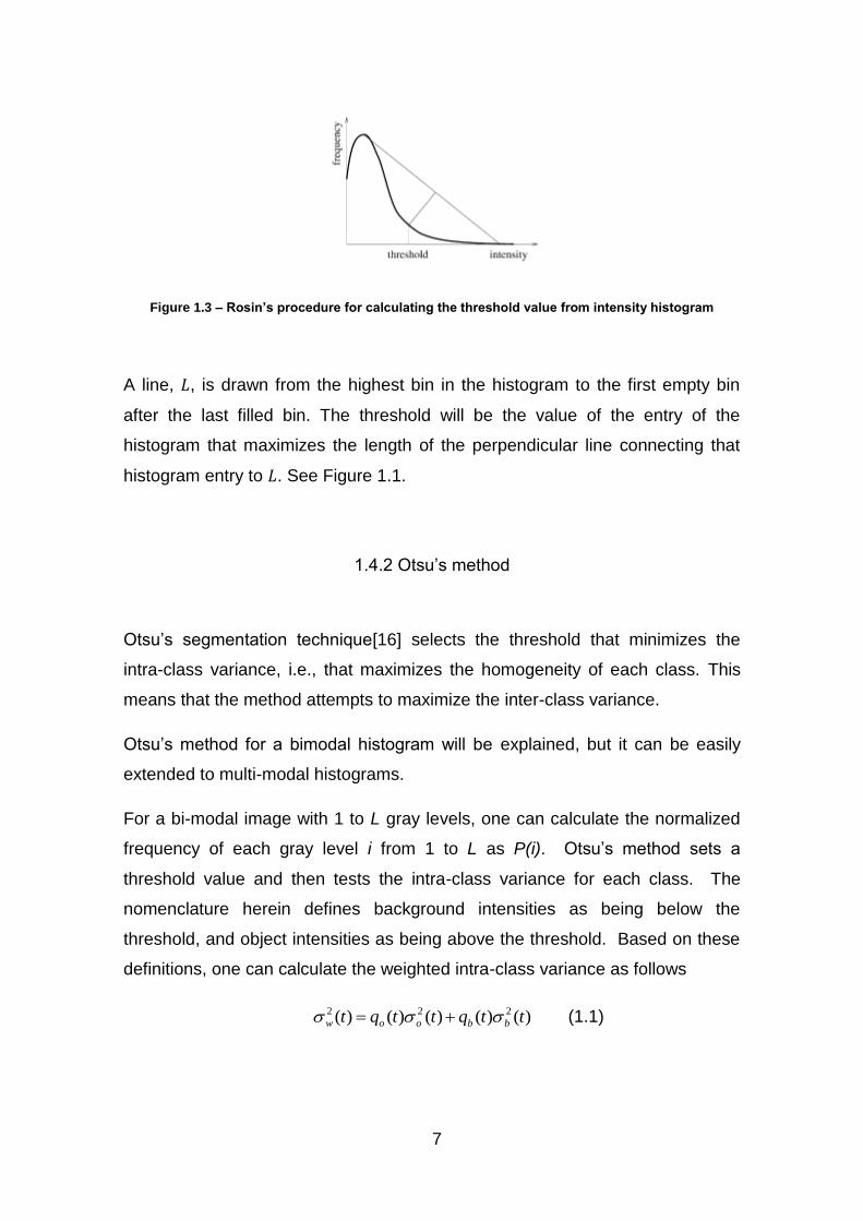
Figure 1.3 – Rosin’s procedure for calculating the threshold value from intensity

histogram............................................................................................................ 7

Figure 2.1 - Ground Truth Evaluation software interface. The cell is displayed

from all three orthogonal axes. ......................................................................... 14

Figure 2.2 - Ground Truth Evaluation software interface with a cell nucleus

boundary traced in red. .................................................................................... 16

Figure 2.3 - Software flow chart ........................................................................ 18

Figure 2.4 - Ground Truth Evaluation software interface. Image shows two

contours drawn on the same slice. The yellow contour is the finished contour;

the red contour is the active contour being drawn. ........................................... 20

Figure 2.5 - Linear Interpolation Illustration ...................................................... 23

Figure 2.6 - Marching Cubes Illustration ........................................................... 24

Figure 2.7 - Marching Cubes’ cubes configuration ........................................... 25

Figure 2.8 - Marching Cubes' configuration cube for when interpolating between

a slice with contour and a slice without contour. ............................................... 26

Figure 2.9 - Delaunay Triangulation's Circumcircle Triangles .......................... 29

Figure 2.10 - Delaunay Triangulation Process ................................................. 30

Figure 2.11 - Representation of True Negative, False Positive, True Positive,

and False Negative Areas ................................................................................ 34

xvi

Figure 3.1 - Nucleus volumes obtained using Linear Interpolation. Top-left

volume obtained with no slices skipped. Top-right volume obtained with 3 slices

skipped. Bottom-left volume obtained with 6 slices skipped. Bottom-right

volume obtained with 9 slices skipped. ........................................................... 39

Figure 3.2 - Nucleus volumes obtained using Marching Cubes. Top-left volume

obtained with no slices skipped. Top-right volume obtained with 3 slices



Figure 3.3 - Nucleus volumes obtained using Gaussian Splat. Top-left volume

obtained with no slices skipped. Top-right volume obtained with 3 slices



Figure 3.4 - Nucleus volumes obtained using Delaunay Triangulation. Top-left




Figure 3.5 - Nucleus volumes obtained using Delaunay Triangulation. Top-left




Figure 4.1 - Jaccard Similarity Index Graph for all five interpolation algorithms 48

Figure 4.2 – Dice Coefficient Graph for all five interpolation algorithms ........... 50

Figure 4.3 - Specificity Index Graph for all five interpolation algorithms ........... 51

Figure 4.4 - Sensitivity Graph ........................................................................... 52

xvii

LIST OF TABLES

Table 3.1 - Inter-user Standard Deviation for nucleus volume ( ) .............. 37

Table 3.2 - Inter-user Standard Deviation for cell volume ( ) ..................... 38

xix

LIST OF ABBREVIATIONS AND ACRONYMS

GUI Graph User Interface

VTK The Visualization ToolKit

1

1. INTRODUCTION

1.1 Motivation

Cancer is a group of diseases characterized by abnormal, unregulated cell

growth. Despite all the extensive research that has been undertaken to better

understand and treat cancer, it is one of the leading causes of death worldwide.

Over 1.6 million new cases, and half a million deaths were estimated in 2012 in

the United States alone [1]. Cancer’s high mortality rate indicates that further

research is needed.

Cancer diagnosis is largely centered on recognizing the morphological

manifestations of the disease, referred to as malignancy associated changes

(MACs)[2]. There are morphological abnormalities that can be observed in the

nuclear structure of cancer cells. Some of the structural differences cancer cells

have when compared to normal cells include nuclear size and shape, number

and size of nucleoli, and chromatin texture[3].

These structures have been studied by growing tumor cells lines in monolayer

tissue culture. Although monolayer culture is easy to work with, it does not

adequately represent the structure of the cell’s nucleus in real tissue; monolayer

culture deforms the nucleus, thus making it fundamental to study these

characteristics using three-dimensional imaging systems[3]. A more accurate

quantitative characterization of cell and nuclear morphology by 3D analysis of

high contrast, high resolution 3D imagery with isotropic resolution facilitates the

assessment of morphological changes associated with malignancy.

Optical microscopy CT is a cellular imaging technique that generates 3D cell

images with an isotropic resolution of 350nm by applying computed tomography

principles and white light excitation[4], [5], as shown in figure 1.1. This is done

by the Cell-CTTM instrument (VisionGate), which generates each cell image by

tomographic reconstruction from five hundred, equi-angular pseudo-projection

2

images acquired over a 360 degree rotation of a stained cell suspended in an

index-matched optical gel (SmartGel, Nye Lubricants) within a glass capillary. A

pseudo-projection image is generated by integrating widefield focal plane

information over the cell volume using a 100x, 1.3 NA, oil immersion objective

lens (UPlanFluor, Olympus). Acquired pseudo-projection images are denoised,

registered and subjected to reconstruction algorithms to generate the volumetric

cell image. The 3D imagining technique used in this research used white light

excitation to image single stained cells and is referred to as single-cell optical

computed tomography (cell CT).

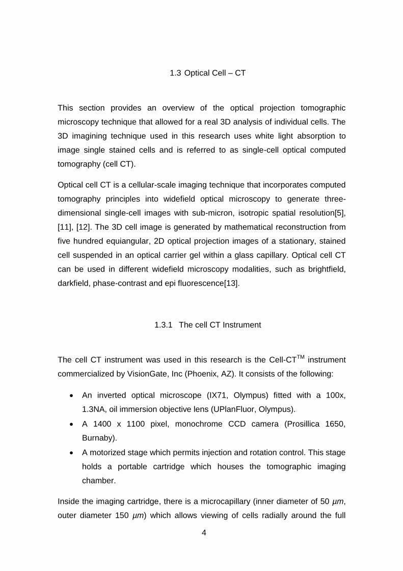
Figure 1.1 - 3D image of a cancer cell generated by the cell CT. Artificial color was added to the nucleus and its components.

Research is being undertaken to precisely quantify three-dimensional cell and

nuclear morphology from cell images generated by optical cell CT imagery and

compute a morphological biosignature composed of the set of morphological

parameters that can best distinguish two or more classes of cells with differing

health states[6]–[8]as seen in figure 1.2. A modular, automated computational

framework is being developed to perform high-throughput, 3D morphological

analysis of volumetric images of Cell-CTTM[9], [10]. Custom 3D image

processing methods are being studied to accurately delineate volumes of

3

interest in the volumetric images, and compute biologically relevant

morphological and texture parameters from the segmented volumes of

interest[10]. The efficacy of these segmentation techniques needs to be

validated by comparison to ground truth. Since size, volume, surface area, and

similar characteristics of a cell cannot be directly measured on the physical cell,

this measurement has to be done using the information contained in 3D

tomographic images.

Figure 1.2 - Four cells imaged using the cell CT. On the top row the nucleus is colored in blue; on the bottom row the nucleus presents a transparency view of the nucleus to show its insides. The first cell is a healthy cell: the subsequent three cells show the progression of different stages of cancer. The progression in nuclear size and morphology, as well as on its components, can be observed.

1.2 Research Goal

Our goal was to develop a method of determining ground truth for 3D cell-CT

image segmentation using interpolation. We present a tool that was developed

in C# that takes advantage of the human ability to visually segment an image

with high accuracy, and converts that information into digital data that can be

used to compare and validate 3D automated segmentation. This research

studied various interpolation methods to make ground truth establishment more

efficient, and determined the interpolation algorithm that allowed for the optimal

ground truth achievement.

4

1.3 Optical Cell – CT

This section provides an overview of the optical projection tomographic

microscopy technique that allowed for a real 3D analysis of individual cells. The

3D imagining technique used in this research uses white light absorption to

image single stained cells and is referred to as single-cell optical computed

tomography (cell CT).

Optical cell CT is a cellular-scale imaging technique that incorporates computed

tomography principles into widefield optical microscopy to generate three-

dimensional single-cell images with sub-micron, isotropic spatial resolution[5],

[11], [12]. The 3D cell image is generated by mathematical reconstruction from

five hundred equiangular, 2D optical projection images of a stationary, stained

cell suspended in an optical carrier gel within a glass capillary. Optical cell CT

can be used in different widefield microscopy modalities, such as brightfield,

darkfield, phase-contrast and epi fluorescence[13].

1.3.1 The cell CT Instrument

The cell CT instrument was used in this research is the Cell-CTTM instrument

commercialized by VisionGate, Inc (Phoenix, AZ). It consists of the following:

An inverted optical microscope (IX71, Olympus) fitted with a 100x,

1.3NA, oil immersion objective lens (UPlanFluor, Olympus).

A 1400 x 1100 pixel, monochrome CCD camera (Prosillica 1650,

Burnaby).

A motorized stage which permits injection and rotation control. This stage

holds a portable cartridge which houses the tomographic imaging

chamber.

Inside the imaging cartridge, there is a microcapillary (inner diameter of 50 µm,

outer diameter 150 µm) which allows viewing of cells radially around the full

5

360º of rotation. The microcapillary is connected to a syringe needle that

permits coupling the Cell-CTTM instrument with a glass syringe. The glass

syringe loaded with stained cells embedded in a carrier gel (Smart Gel, Nye

Lubricants) is connected to the syringe needle of the Cell-CTTM, and an injection

controller is connected to the other end of the glass syringe to carefully control

the disbursement of the sample into the microcapillary. All the elements in the

imaging chamber, including the capillary and the carrier gel, and the immersion

oil for the objective lens are refractive index matched to minimize optical

distortion.

A LabView software suite is used to automate the image acquisition process.

1.3.2 Projection Image Acquisition

Once the glass syringe with the stained cells is mounted onto the Cell-CTTM, the

cells are transported through the capillary by forward actuation of the syringe

plunger. This pressurizes the carrier gel and causes it to flow. When a desired

cell is in the field of view of the microscope, the pressure is released and the gel

flow stops; making the cell immediately stationary. The user selects the cells to

be imaged based on cell quality. If a cell is selected to be imaged, the capillary

will rotate at constant speed, allowing the acquisition of 500 projection images

at angular intervals of 0.72º around the cell. Each projection image is generated

by sweeping the objective lens through the cell volume and integrating the

resultant infinite focal plane information on the camera chip[12].

A 3D image is generated by aligning the projection image data, and subjecting it

to mathematical reconstruction algorithms. To eliminate pattern noise, a

background subtraction routine is performed. The alignment is done based on

the center of intensity; the aligned projections are subject to filtered back

projection reconstruction using a custom ramp filter to obtain the volumetric cell

image. This image has an isotropic spatial resolution of ~350nm.

Reconstructed volumes are stored as 2D image stacks at bitdepths of 8 and

16bits. Intensities in the reconstructed image inversely correlate with

6

hematoxylin stain density, i.e. a darker stain implies a higher intensity in the

image.

1.4 Segmentation Algorithms

Automated segmentation algorithms for medical images have been a subject of

active research. Many techniques have been developed[14] and are being

evaluated. In a collaborative effort, a fellow laboratory colleague developed a

fully-automated segmentation algorithm to segment the cell CT images. The

segmentation algorithms chosen to be used in his research were the ones

considered to be the most adequate after analyzing the characteristics of the

cell CT image[10]. For brevity, only the segmentation methods used in the cell

CT research will be exposed. The ground truth that is produced from this project

was used to validate these automated segmentation algorithms.

1.4.1 Rosin’s threshold method

Threshold segmentation algorithms segment an image based on its histogram.

Different modal classes can be identified on a histogram; and the key to

segmentation based on threshold is to identify the value, i.e. the threshold, that

best separates the different modal classes.

Rosin’s method[15] assumes that the image’s histogram is unimodal. This

means that there is one dominant class that will result in one peak at the lower

end of the histogram, and the secondary class will be more spread out in the

higher end of the histogram.

7

Figure 1.3 – Rosin’s procedure for calculating the threshold value from intensity histogram

A line, , is drawn from the highest bin in the histogram to the first empty bin

after the last filled bin. The threshold will be the value of the entry of the

histogram that maximizes the length of the perpendicular line connecting that

histogram entry to . See Figure 1.1.

1.4.2 Otsu’s method

Otsu’s segmentation technique[16] selects the threshold that minimizes the

intra-class variance, i.e., that maximizes the homogeneity of each class. This

means that the method attempts to maximize the inter-class variance.

Otsu’s method for a bimodal histogram will be explained, but it can be easily

extended to multi-modal histograms.

For a bi-modal image with 1 to L gray levels, one can calculate the normalized

frequency of each gray level i from 1 to L as P(i). Otsu’s method sets a

threshold value and then tests the intra-class variance for each class. The

nomenclature herein defines background intensities as being below the

threshold, and object intensities as being above the threshold. Based on these

definitions, one can calculate the weighted intra-class variance as follows

)()()()()( 222 ttqttqt bboow (1.1)

8

where w refers to the weighted intra-class variance, t refers to the threshold

value, o refers to the object class from the image, b refers to the background

class from the image, σ is variance, and q is intra-class probabilities. These

intra-class probabilities are estimated as follows:

t

i

o iPtq1

)()( (1.2)

and

I

ti

b iPtq1

)()( (1.3)

such that 1)()( tqtq bo .

In addition, the class means are computed by the following:

t

io

o iiPtq

t1

)()(

1)( (1.4)

and

I

tib

b iiPtq

t1

)()(

1)( (1.5)

Finally, the variance of the background and object classes can be computed as

follows:

t

i

o

o

o iPtitq

t1

22 )()]([)(

1)( (1.6)

and

I

ti

b

b

b iPtitq

t1

22 )()]([)(

1)( . (1.7)

Simply, the threshold for every possible pixel value could be assigned to t, and

a minimum σw could be selected from all of the possible computations.

However, taking advantage of the fact that the total variance for the entire

image σ is equal to the weighted intra-class variance σw and the weighted inter-

9

class variance σB—which is merely a relationship between the weighted

distances between the class means and the grand mean of the entire dataset

μ—one can rewrite the equations above as follows.

222 ])()[(])()[()( ttqttqt bbooB (1.8)

and

)()( 222 tt Bw (1.9)

Since the overall variance does not change for the dataset depending on the

threshold, one can see that minimizing the intra-class variance is equivalent to

maximizing the inter-class variance to arrive at an optimum threshold.

1.4.3 K-means Clustering

In order to cluster data in a way such to minimize an objective function, k-

means clustering methodologies can be used[17], [18]. In these methodologies,

n observations can be broken into k partitions such that each observation

belongs to the cluster with the nearest mean; in other words, the within-cluster

sum of squares or the mean squared distance of each observation to the mean

of the cluster in which it falls is minimized.

In application to image analysis, this can be viewed as breaking the pixels of an

image into two or more partitions based on the intensity of the pixels. While

computationally difficult, k-means clustering has proven very efficient when

subjected to heuristic methods. Primarily, the segmentation algorithm can be

used to approximate this methodology by assuming the optimal center for a

cluster of data falls at the centroid of that data cluster. The mean-squared

distance from each point to the mean of the cluster can be computed; then the

various clusters’ final mean-squared distance computations can be summed. A

slightly different set of clusters is estimated from the dataset, and then the

centroid for each cluster is recomputed along with the mean-squared distance

from each point to the mean of each cluster. The final summed mean-squared

10

distance computations for the new cluster set can be summed and compared to

the previous iteration. When the objective function—i.e., the sum of all of the

within-cluster sum of squares—is minimized, then the optimal formulation of the

clusters has been found to minimize intra-class variability.

Given a set of observations (x1, x2, …, xn), where each observation is a d-

dimensional real vector, k-means clustering aims to partition the n observations

into k sets (k ≤ n) S = {S1, S2, …, Sk} so as to minimize the within-cluster sum of

squares (WCSS):

(1.10)

where μi is the mean of points in Si.

1.5 State of the Art

With the increasing use of 3D imaging techniques in the medical field, it is

crucial to understand and manipulate the data and vital information present in

these images. Image segmentation is widely used in many imaging modalities

in various different medical fields. A few software applications have been

developed that allows for manual segmentation of a 3D medical image.

TurtleSeg is a free 3D medical image segmentation tool developed by the

Medical Image Analysis Lab at Simon Fraser University and the Biomedical

Signal and Image Laboratory at the University of British Columbia[19].

The software allows the user to manually segment a sparse number of slices.

The software picks the slices that are crucial to be manually traced for the user

to draw; and then calculates the volume by producing a dense set of parallel

segmentation contours.

TurtleSeg was developed to be used with a mouse. Since it is hard to trace a

contour with a mouse, TurtleSeg uses a livewire. The user does not need to

11

trace the contour perfectly, instead the user clicks on relevant points and

livewire connects the sequential cliked points.

ITK–Snap is a free software application to segment 3D medical images

developed by Paul Yushkevich, Ph.D., of the Penn Image Computing and

Science Laboratory (PICSL) at the Department of Radiology at the University of

Pennsylvania [20].

Unlike TurtleSeg, ITK-Snap allows the user to draw on all the slices, and have

fully manual segmentation. This software application was also developed to be

used with a mouse, so it also has a livewire where you can add as many points

as needed to make the shape as close as possible to the desired contour. Once

you are done with one slice and move to the next, the contour drawn on the

previous slice will appear on top of the image. Since there is not much change

between slices, the user can use that as a guide and only make small changes

to the contour; making the process of tracing the contours faster.

3D-Doctor is a 3D medical image processing tool used in many organizations

working with medical images. Unlike the previous two, this tool is not free. 3D-

Doctor allows the user to manually segment all the slices of a 3D image by

clicking the mouse around the desired boundary on each slice[21].

Studies have shown that manual segmentation using a pen and a tablet are

easier, faster and more accurate[22]. Even though this technique has been

used in several medical research fields[23], [24], we do not know of any freely

available software developed to be used with a pen and tablet that does 3D fully

manual segmentation.

Our software will be innovative in that it is designed to be used with a pen and

tablet, the user can pick what slices he/she intends to draw on, being able to

draw on all slices or only draw on a few, and it uses interpolation to speed up

the process of obtaining a volume.

http://picsl.upenn.edu/

http://picsl.upenn.edu/

13

2. METHODS

2.1 Cell Sample Preparation

The cells used for imaging were grown in culture. This research analyzed

different kinds of cancer cells as well as healthy cells. After the cells were

grown, they had to be prepared for imaging.

The optical contrast must be proportional to the density of the biological

material, since, like x-ray CT, the cell CT 3D image captures variations in the

object’s density. To achieve this, the cell needs to be stained with an absorption

dye. The dye used was hematoxylin, commonly used in clinical practices for this

purpose[25]. Standard cytological protocols for staining were followed as

outlined below.

Staining Procedure:

1. Cells are fixed for one hour with CytoLyt, and posteriorly smeared onto a

clean microscope glass slice coated with a Poly-L-Lysine solution.

2. Cells are stained for a few minutes (cell type dependent) in aqueous

6.25% w/w Gill’s hematoxylin solution, followed by a bluing reagent

(Fisher Scientific, Fair Lawn) for 30 seconds after washing thrice with

filtered tap water.

3. Cells are dehydrated by use of an ethanol series (50%, 95%, and 100%)

and two washes of xylene.

After the cells are stained they are embedded into the carrier gel and scraped

off the glass slide to be introduced into the glass syringe.

It is important to optimize the staining results, since the imaging quality is

dependent on it. To accomplish this, various trials are needed to determine

optimal concentration of reagents and the duration of protocol steps, since the

14

optimization of the results is so dependent on experimental conditions (including

pH of the water used).

The properly stained cells will have a bluish nucleus and a lighter cytoplasm.

The staining is more predominant in the nucleus due to binding of the dye-metal

to nuclear DNA.

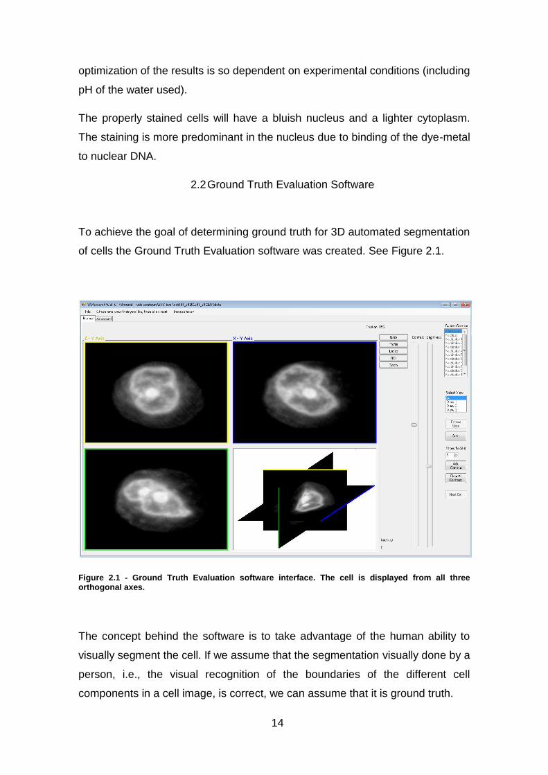
2.2 Ground Truth Evaluation Software

To achieve the goal of determining ground truth for 3D automated segmentation

of cells the Ground Truth Evaluation software was created. See Figure 2.1.

Figure 2.1 - Ground Truth Evaluation software interface. The cell is displayed from all three orthogonal axes.

The concept behind the software is to take advantage of the human ability to

visually segment the cell. If we assume that the segmentation visually done by a

person, i.e., the visual recognition of the boundaries of the different cell

components in a cell image, is correct, we can assume that it is ground truth.

15

The real challenge is to convert the result from the visual segmentation into

digital data that can be compared with the result of the automated

segmentation. This is best performed by utilizing a tablet and a pen to draw on

the images of the cell. In this way, a user of the Ground Truth Evaluation can

input his/hers visual segmentation into the software by drawing a contour

around the identified boundary.

For this purpose, the tablet Cintiq 12wx (Wacom) was used. The Wacom Cintiq

12wx is a 12.1" TFT wide-screen LCD in WXGA resolution of 1280 x 800 pixels.

The goal was to have a 3D segmentation of the cell’s components, but we were

limited to a 2D display and therefore limited to 2D images. For this reason, the

3D image has to be divided into a series of slices; where each slice represents

a 2D image. This is simple, if we consider that a 3D image is a stack of 2D

images. The data of the 3D image is stored in a 3D matrix. A 3D matrix of the

type can be written as matrices of the type . So a 3D matrix can

be decomposed into a series of 2D matrices. Each 2D matrix defines a 2D

image that is one slice of the 3D image.

The Ground Truth Evaluation will go through the stack of 2D images, and the

user can then draw a contour on each slice. This contour will define the

segmentation for that slice. After the user has defined the segmentation

boundary of the desired object on every slice, the slices can be stacked back

into a 3D volume. This will allow for a full 3D segmentation, since all the planes

of the 3D volume were segmented.

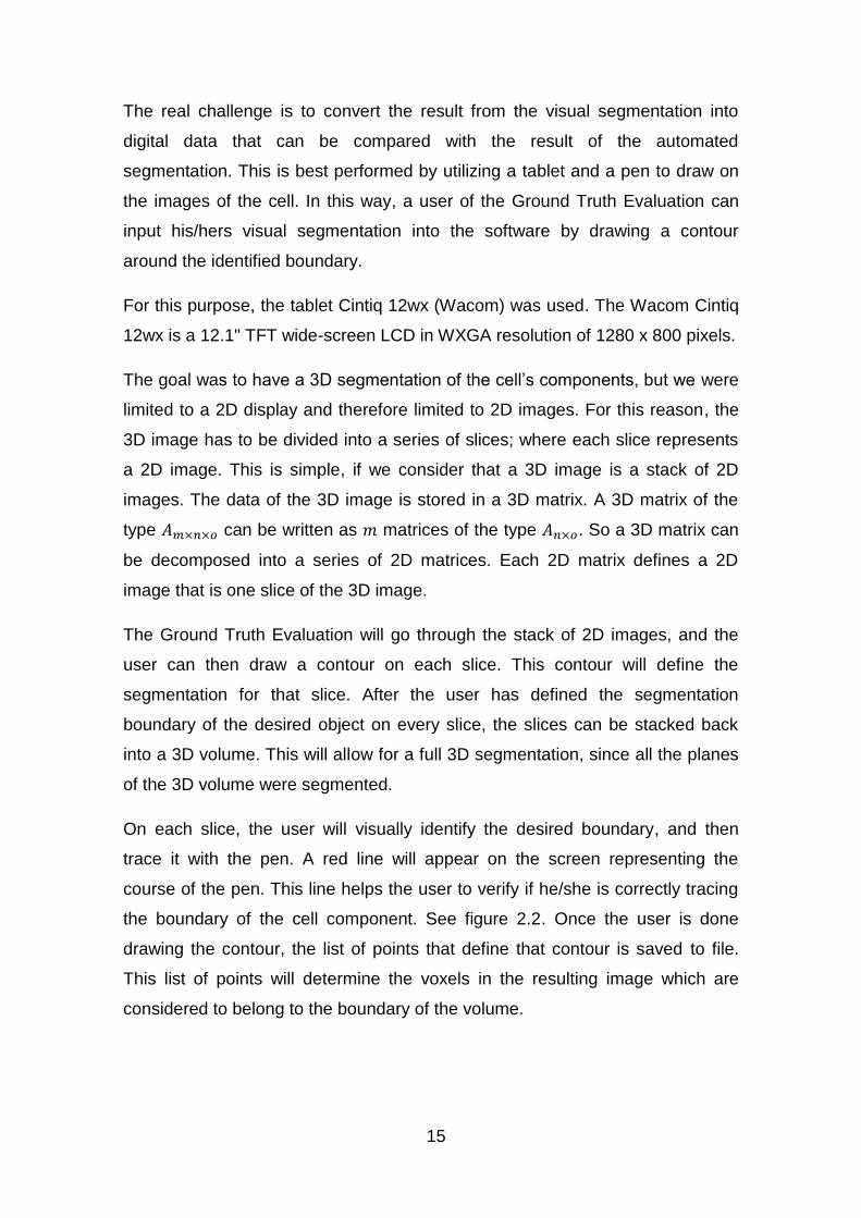
On each slice, the user will visually identify the desired boundary, and then

trace it with the pen. A red line will appear on the screen representing the

course of the pen. This line helps the user to verify if he/she is correctly tracing

the boundary of the cell component. See figure 2.2. Once the user is done

drawing the contour, the list of points that define that contour is saved to file.

This list of points will determine the voxels in the resulting image which are

considered to belong to the boundary of the volume.

16

Figure 2.2 - Ground Truth Evaluation software interface with a cell nucleus boundary traced in red.

Once the boundary of the volume is defined on a slice, the section of volume on

that slice can be determined with a flood fill algorithm. This algorithm

determines all the pixels enclosed in a bounded area. In this way, all the pixels

of that image that are contained in the volume are found. The total volume of

the ground truth is the sum of all the voxels belonging to the volume in each

slice.

Even though this method of determining ground truth is reliable, there is one

problem with it: it is too slow. To precisely draw one contour, it takes between

30 seconds to 1 minute. A cell, depending on the size of the cell and along

which axis the user chooses to draw, will require around 170 slices. This means

it takes over two hours to draw the contours of just one of a cell’s components.

So the next step in the development of this software becomes to create a way

to make this process faster. This goal can be achieved through interpolation.

This means that the user does not need to draw on every slice. Instead, the

user can skip slices, and only draw on a selected number of slices. Using an

interpolation algorithm, the software will interpolate the volume between the

17

slices that were skipped. In this way, it is possible to obtain the ground truth

volume without needing to define its boundary on every slice, making it a much

faster process.

Different interpolation methods and algorithms will be discussed in the next

section.

After the ground truth volume is found, it is then possible to compare it with the

volume resulting from automated segmentation algorithms. The Ground Truth

Evaluation has a few evaluation metrics that can be applied to the volumes to

compare and evaluate how close the automated segmentation came to the

ground truth volume.

These metrics will be presented in section 2.4. They will also be used to

evaluate the interpolation methods.

The software provides a full pathway for the evaluation, segmentation, and

eventual rating of the cell and the automatic segmentation as shown in figure

2.3.

18

Figure 2.3 - Software flow chart

Some extra features that were added to the software include:

The ability to zoom – the user can zoom in and out in the image, making

it easier to define the boundaries.

The ability to change the contrast – the user can adjust the contrast of

the image optimizing the visualization of the cell and its components.

The ability to change the brightness – the user can adjust the brightness

of the image optimizing the visualization of the cell and its components.

The user can select what cell component (Cell Wall, Nucleus, Nucleolus

1, Nucleolus 2, etc…) he/she is drawing. The name of that component

will be tied to all the contours belonging to it. In this way, it is only

necessary to load the cell once to draw all the different cell components.

All of the cell’s components for a given cell can be saved in one file.

When the cell is loaded, the user can see the cell from the perspective of

all three axes. The user can move through the stack on each axis and

choose which view he/she would like to work with. See Image 2.1.

Evaluation of Automated Segmentation

The ground truth volume can be used to compare and evaluate the validity of other segmentatios. This can be done using different evalution metrics.

Ground Truth Volume

The ground truth volume is obtained.

Interpolation

The software will interpolate the volume between the slices that were drawn on.

User draws contours

The user will go through the stack of images drawing the contours on the slices that were not skipped.

Load the Cell Image

View from the 3 axis are shown. The user can scan through the cell stack and select the axis on which he/she desires to draw on.

User defines number of slices to be skipped

19

Setting the number of slices to be skipped – the user can predefine how

many slices he/she desires to skip before starting to draw. In this way,

every time the user selects the “Next Slice” button the software will

automatically skip the desired number of slices, and display the

corresponding slice image.

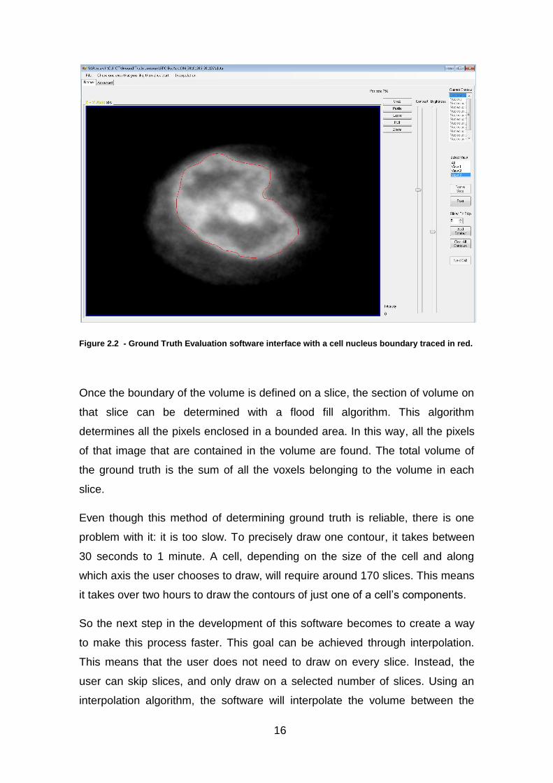
The possibility of drawing multiple contours on the same slice – this in an

important feature. The cell components can have different cell shapes. In

some cases, the shape can include variations like large dents in the

surface. These dents can produce two parallel saliencies that project out

in the same direction but do not touch each other. This will imply that

when this object is divided into slices, there will be slices where it

appears as two different objects. This is easy to picture if you consider

slicing horizontally a U-shaped object. It becomes a problem to draw a

contour around the surface of a cell component which in a given slice

appears as two disjointed objects, even though both segments belong to

the same object. To overcome this problem, the software allows the user

to draw multiple contours for the same cell component on a given slice.

When the user is satisfied with the first contour, he/she can select the

“Add Contour” button to draw another contour. The finished contours will

appear yellow, and the current contour being drawn will be red. See

Figure 2.4.

Each contour has to be traced continuously. If the user dislikes the line

traced all he/she has to do is take the pen off the screen and then

proceed to restart tracing the surface. This will clear the image of the line

of the previous attempt. Other contours drawn on that slice that are now

yellow will not be cleared by this action. Only the current contour being

drawn is cleared. To clear all contours, the user can select the “Clear All

Contours” button.

The user can go back to previous slices that were drawn on. When

he/she does so, he/she will be able to visualize the contour(s) drawn on

that slice and can redraw them if wanted.

20

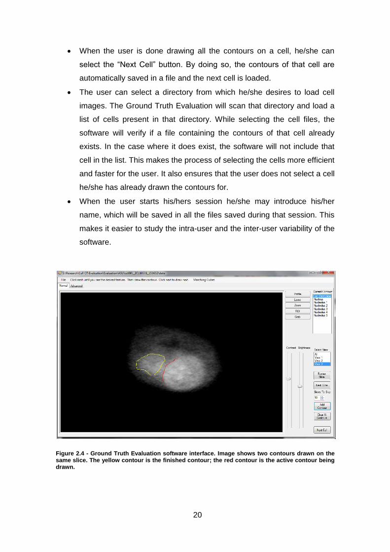
When the user is done drawing all the contours on a cell, he/she can

select the “Next Cell” button. By doing so, the contours of that cell are

automatically saved in a file and the next cell is loaded.

The user can select a directory from which he/she desires to load cell

images. The Ground Truth Evaluation will scan that directory and load a

list of cells present in that directory. While selecting the cell files, the

software will verify if a file containing the contours of that cell already

exists. In the case where it does exist, the software will not include that

cell in the list. This makes the process of selecting the cells more efficient

and faster for the user. It also ensures that the user does not select a cell

he/she has already drawn the contours for.

When the user starts his/hers session he/she may introduce his/her

name, which will be saved in all the files saved during that session. This

makes it easier to study the intra-user and the inter-user variability of the

software.

Figure 2.4 - Ground Truth Evaluation software interface. Image shows two contours drawn on the same slice. The yellow contour is the finished contour; the red contour is the active contour being drawn.

21

The software realization was achieved by programming in C#. C# is a

programming language developed for .NET Framework[26].

There were several aspects of the C# programming language that were

attractive and are the reasoning to why it was chosen over other languages.

Some of these aspects are listed below:

Allowing polymorphism in object-oriented programming. This means that

methods can be implemented to work with groups of related objects in a

uniform way. In other words, it is possible to present the same interface

for different underlying data types. This made it possible to organize the

data into classes and subclasses, and take advantage of inheritance,

making the Ground Truth Evaluation more efficient.

3D Libraries – C# has an extensive library for 3D graphics, something

that was vital for the Ground Truth Evaluation.

C# makes it easy to work with plug-ins. This makes it possible to work

with the Ninject design pattern, which was used to make the drawing and

lasso tools.

Easy to create and work with Graphical User Interface (GUI) – The

Ground Truth Evaluation relies on the functionality of GUIs.

Reflection – the ability to inspect and determine the contents of an

unknown assembly, object, type, and members. This is useful for

determining dependencies of an assembly, testing and debugging.

The Visualization Toolkit (VTK)[27] library was integrated into the Ground Truth

Evaluation. VTK is an open-source C++ library used in 3D computer graphics,

image processing and visualization. VTK is a very useful tool in computer

graphics making it easier to perform complex tasks using an object-oriented

approach. This software system is widely used due to its compatibility with other

languages like Tcl/Tk, Java and Python. VTK was chosen over other 3D

computer graphics libraries such as OpenGL and DirectX because of its

modular, object-oriented and scalable proprieties. VTK is also geared more

specifically for scientific use.

The Ground Truth Evaluation is modular for reusability. This means that the

code is organized into modules that can be easily used to add, delete or modify

22

functionalities to the code without much effort or coding. This makes it easy to

integrate the software into other software and scripts.

2.3 Interpolation Algorithms

In this section, five different interpolation algorithms are presented to complete

the volume between the slices that were drawn on.

2.2.1 Linear Interpolation

The concept behind Linear Interpolation is simple. All the slices of the 3D image

are introduced into the algorithm. The algorithm will find the slices that contain

at least one contour. For each point in a given contour (contour A) the nearest

point to it in the next contour (contour B) is found. The straight line that

connects the two points is calculated. That line will then intersect all the planes

defined by the slices in between the drawn slices containing contours A and B.

In this way, a point is defined on each intersected slice, see Figure 2.5. This

process is repeated for all the points in contour A, creating a set of points on

each intersected slice. The set of points on a given slice will define a new

contour on that slice. A contour on all the slices that were skipped is created.

The interpolated volume is then the result of all the contours.

23

Figure 2.5 - Linear Interpolation Illustration

The mathematics behind this method is simple and does not require much

computationally. It is a robust method that will work for any kind of complex cell

shape.

On the other hand, it is important to note that this method does not have any

surface awareness. It does not recognize patterns in the shape of the volume

and will not try to reproduce it. It also fails to produce curvature on the undrawn

slices, something that is expected in the shape of cells. The Linear Interpolation

will generate a volume that is smaller than that of the ground truth, since it will

not recreate the curves of the cell, but only the flat lines between slices. This will

also result in a volume with sharp edges.

It is also important to take into account that the Linear Interpolation only

interpolates between slices. It cannot interpolate before the first slice that was

drawn on, or after the last slice that was drawn on. This means that the ends of

the cell may be cut off. With this in mind, the user should always try to draw on

the first slice where the cell is seen, as well as on the last one.

To understand how this algorithm was implemented see pseudo-code in

Appendix A.1.

24

2.2.2 Marching Cubes

Marching Cubes is an algorithm used in computer graphics to construct and

display 3D data. It creates a polygonal mesh from an isosurface within the 3D

data[28].

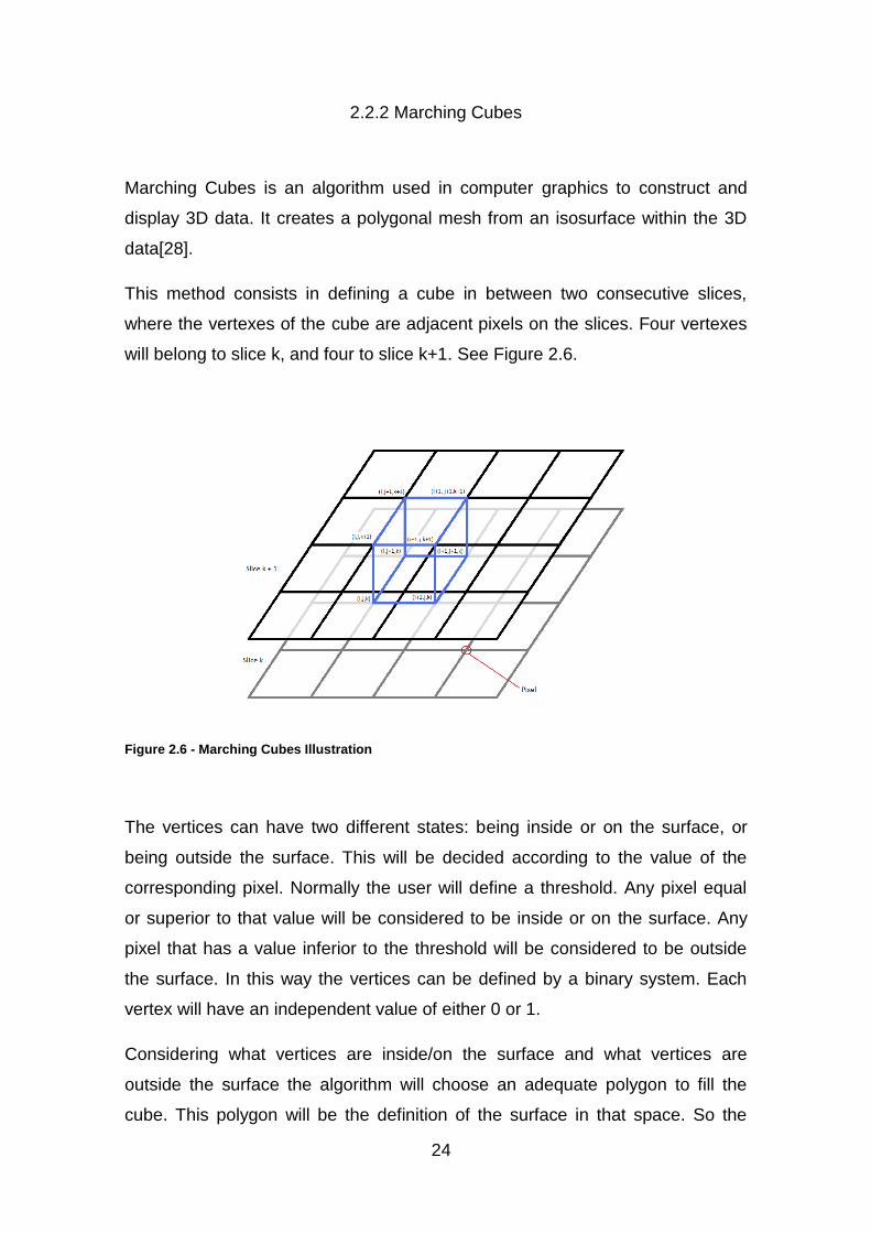
This method consists in defining a cube in between two consecutive slices,

where the vertexes of the cube are adjacent pixels on the slices. Four vertexes

will belong to slice k, and four to slice k+1. See Figure 2.6.

Figure 2.6 - Marching Cubes Illustration

The vertices can have two different states: being inside or on the surface, or

being outside the surface. This will be decided according to the value of the

corresponding pixel. Normally the user will define a threshold. Any pixel equal

or superior to that value will be considered to be inside or on the surface. Any

pixel that has a value inferior to the threshold will be considered to be outside

the surface. In this way the vertices can be defined by a binary system. Each

vertex will have an independent value of either 0 or 1.

Considering what vertices are inside/on the surface and what vertices are

outside the surface the algorithm will choose an adequate polygon to fill the

cube. This polygon will be the definition of the surface in that space. So the

25

polygon has to ensure to include all the vertices that were labeled as inside the

surface in the surface; as well as exclude from the surface all the vertices that

were labeled as outside the surface.

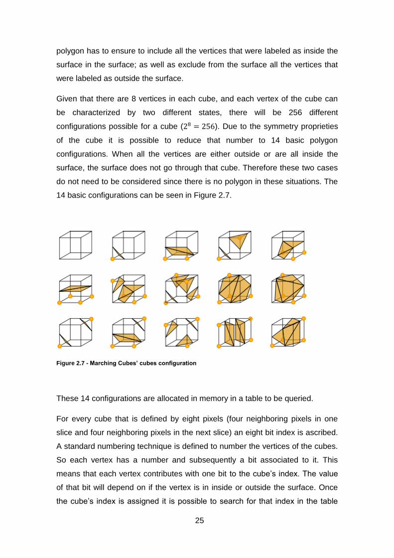
Given that there are 8 vertices in each cube, and each vertex of the cube can

be characterized by two different states, there will be 256 different

configurations possible for a cube ( ). Due to the symmetry proprieties

of the cube it is possible to reduce that number to 14 basic polygon

configurations. When all the vertices are either outside or are all inside the

surface, the surface does not go through that cube. Therefore these two cases

do not need to be considered since there is no polygon in these situations. The

14 basic configurations can be seen in Figure 2.7.

Figure 2.7 - Marching Cubes’ cubes configuration

These 14 configurations are allocated in memory in a table to be queried.

For every cube that is defined by eight pixels (four neighboring pixels in one

slice and four neighboring pixels in the next slice) an eight bit index is ascribed.

A standard numbering technique is defined to number the vertices of the cubes.

So each vertex has a number and subsequently a bit associated to it. This

means that each vertex contributes with one bit to the cube’s index. The value

of that bit will depend on if the vertex is in inside or outside the surface. Once

the cube’s index is assigned it is possible to search for that index in the table

26

that contains all possible polygon configurations. Each configuration will have a

list of all possible indexes associated with that specific configuration.

After the surface shape is found for a cube, the intersection of that surface with

the edges of the cube is calculated. This calculation is done by linear

interpolation using the vertex’s density value. Each cube defines the surface in

that space, the total volume is the combination of all the surfaces enclosed in

each cube.

The final step is the calculation of the triangles’ in each cube normal. This is

useful for rendering algorithms to produce shading in the surface.

For interpolation purposes, not all slices are introduced into the Marching Cube

algorithm. Only the slices with contours are introduced. The slices that were

skipped are removed from the volume. The Marching Cubes algorithm is

applied to the slices that contain a contour as if they defined the whole volume.

Once the surface is created using the Marching Cubes algorithm the surface is

stretched back out to the original volume size. This will elongate the polygons

along the axis perpendicular to the slices. This elongation will result in less

resolution along that axis compared to the other two axes. This technique is the

standard in computer graphics and is used for a wide range of applications. It is

a robust method that works for different kinds of data.

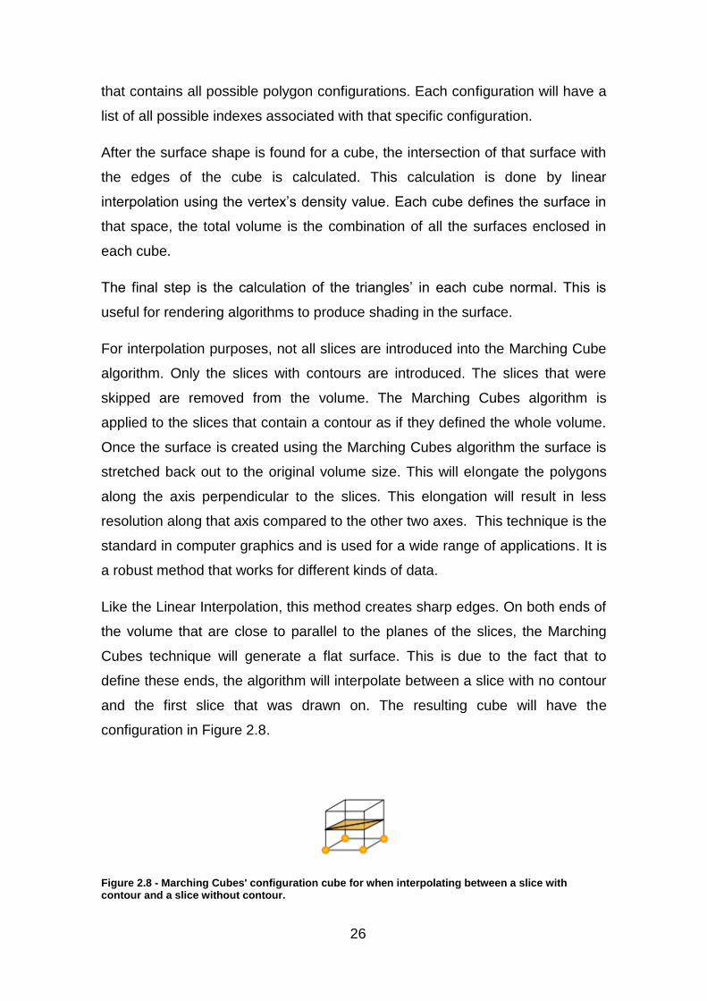
Like the Linear Interpolation, this method creates sharp edges. On both ends of

the volume that are close to parallel to the planes of the slices, the Marching

Cubes technique will generate a flat surface. This is due to the fact that to

define these ends, the algorithm will interpolate between a slice with no contour

and the first slice that was drawn on. The resulting cube will have the

configuration in Figure 2.8.

Figure 2.8 - Marching Cubes' configuration cube for when interpolating between a slice with contour and a slice without contour.

27

This will mean that the surface will be flat in those extremes.

Marching Cubes is a computationally expensive algorythm since it requires a

secondary interpolation and a large amount of memory needs to be allocated

due to the fact that the vertices are not connected until the calculation is

completed.

To understand how this algorithm was implemented see Appendix A.2.

2.2.3 Gaussian Splat

Splatting techniques[29] use a splatting function to distribute the data value of

each point over the surrounding region. This is done using a splatting kernel, or

blur kernel. The kernel should be symmetric and gradually decrease to zero as

you move away from the centre. In this way, the algorithm will blend all the

volume points. It is important to assure that the kernel has an adequate size. A

kernel that is either too big or too small can produce artifacts in the surface,

such as blurring and loss of detail.

The Gaussian Distribution Function can be used as a splatting function. The

Gaussian function is the probability density function of the normal distribution,

which in 3D is expressed as:

where is the standard deviation and µ the mean.

The Gaussian Distribution Function can be used to distribute a point to its

surrounding. This is done by creating a Gaussian distribution around each point,

where the point is the mean, µ, of the distribution, or the “peak” of the Gaussian

28

curve. The Gaussian distribution for a given point will be the contribution of that

point to the volume. In this way, each point will define a small volume in the 3D

space. The sum of all the volumes defined by each point will be the final

volume.

The Gaussian Distribution Function, centered on a given point , can be written

as:

(2.2)

where is the distance from to , ,

is the radius of propagation of the splat, this value is expressed as a

percentage of the length of the longest side of the sampling volume,

and is the scalar value of point .

This function is used in the Gaussian Splat interpolation technique. The function

is applied to the list of points to be interpolated. Once the values have been

blurred, an isosurface is extracted from the volume. This interpolation

technique will work for any kind of input contours and is very robust and fast.

The Gaussian Splat will create a volume larger than the ground truth volume.

Since the interpolation is calculated by expanding each point into its

surroundings, it will expand the whole volume. Unlike Linear Interpolation and

Marching Cubes, Gaussian Splat will not produce a volume with sharp edges.

Instead, it will create a volume with large rounded edges. It also will remove

any trace of fine features.

2.2.4 Delaunay Triangulation

29

Delaunay Triangulation[30] is used in computer graphics to create geometric

surfaces from a list of points, . This is done by defining

edges of triangles between points and, consequently, connecting all the points

through triangles. The edges should never intersect each other. This method

will produce a surface made up of various small triangles, where the vertices of

these triangles are the points belonging to .

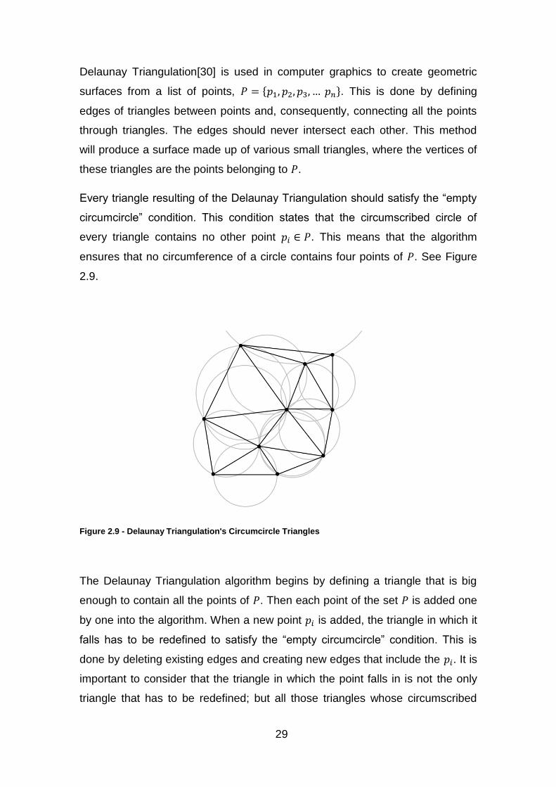
Every triangle resulting of the Delaunay Triangulation should satisfy the “empty

circumcircle” condition. This condition states that the circumscribed circle of

every triangle contains no other point . This means that the algorithm

ensures that no circumference of a circle contains four points of . See Figure

2.9.

Figure 2.9 - Delaunay Triangulation's Circumcircle Triangles

The Delaunay Triangulation algorithm begins by defining a triangle that is big

enough to contain all the points of . Then each point of the set is added one

by one into the algorithm. When a new point is added, the triangle in which it

falls has to be redefined to satisfy the “empty circumcircle” condition. This is

done by deleting existing edges and creating new edges that include the . It is

important to consider that the triangle in which the point falls in is not the only

triangle that has to be redefined; but all those triangles whose circumscribed

30

circle contains . This procedure is repeated until all the points are successfully

integrated into the Delaunay Triangulation. After all points are added, the edges

that connect the points of the initial triangle created to contain all the points of

can be eliminated. Figure 2.10 shows how this process is done.

Figure 2.10 - Delaunay Triangulation Process

Even though it was shown how the Delaunay Triangulation works in 2D, the

concept still holds in 3D, where , and the algorithm defines 3D simplexes

and their corresponding circumscribed spheres.

This method is widely used in computer graphics. It is a very efficient method to

extract surfaces from a list of points. It works best for points that are spread out

evenly in space, where the points are not agglomerated. If the set of points is

too dense, the algorithm has difficulties in defining the simplexes. The ideal

scenario for the Delaunay Triangulation is that where, for a set of points in a

31

plane, no three points lie on the same line and no four points lie on the same

circle.

The points to which the algorithm is applied in this case is the list of points that

define the contours drawn by the user. A contour, theoretically, is defined by an

infinite number of points. This list of points will be a string of consecutive points

to describe a continuous line. The fact that there is no spacing between the

points is a problem for the Delaunay algorithm. Even though the algorithm will

exclude points that coincide or almost do so, it will still have to define edges

between points that are too close together and their almost infinite

circumscribing circles. It is very unlikely that the data obeys the condition for the

ideal scenario mentioned on the previous paragraph.

For this technique, the number of points introduced into the algorithm was

reduced to improve its performance. No great improvement was noticed in its

behavior.

2.2.5 Unorganized Points

Unorganized Points [31] is a very sophisticated surface reconstruction

algorithm. Considering M as the unknown surface that we intend to calculate,

function f

, (2.3)

can be defined, where is a region near the data. The function f

estimates the signed geometric distance to M. The zero set is the estimate

for M. A contouring algorithm is then used to approximate by a simplicial

surface.

32

The first step consists of attributing an oriented tangent plane to each data

point , where X is set of data points. These planes serve as a local linear

approximation of the surface, and will be used to help calculate for .

The singed distance of a point p to a surface M is the distance between p and

the closest point , multiplied by . Multiplying it by allows

distinguishing points that are on different sides of the surface. Since M is not

known the oriented tangent planes are used for this calculation. The distance of

p to M is defined as the distance from p to the plane which has the

center closest to p; that is,

, (2.4)

where is a unit normal vector.

Once the zero set is found a contouring algorithm can be used to

discretely sample the function f over a portion of a 3D grid near the data and

reconstruct a continuous piecewise linear approximation to The contour

tracing algorithm used to extract the isosurface from the scalar function is the

algorithm of Wyvill et al..

2.4 Evaluation Metrics

To evaluate the performance of each interpolation algorithm, we drew the

contours of a cell nucleus on every slice. We then used those contours to

generate a volume using each interpolation method. Ten iterations of this

process were done; where, in each iteration, one more slice was skipped than

in the previous iteration. That is, on the first iteration, all contours were used to

obtain the volume; on the second, only every other contour was used, making

the number of slices skipped 1; on the third, only every third contour was used,

33

making the number of slices skipped 2; and so on, until the number of slices

skipped was 9.

The evaluation metrics used to evaluate the interpolation methods were Jaccard

Similarity[32], Dice Coefficient[33], Specificity and Sensitivity[34]. These metrics

are the same metrics that the Ground Truth Evaluation software has built in to

evaluate the fully-automated segmentation algorithms.

For a better comprehension of the metrics, the following terminology will be

used:

V - all the voxels in the image;

GT (ground truth) – all the voxels classified as cell by the user;

I (interpolated volume) – all the voxels classified as cell by the

interpolation method;

TP (True Positive) – all the voxels that were classified as cell by both the

user and the interpolation method, i.e., ;

TN (True Negative) – all the voxels that were classified as non-cell by

both the user and the interpolation method, i.e., ;

FP (False Positive) – all the voxels that were classified as non-cell by the

user but were classified as cell by the interpolation method, i.e.,

;

FN (False Negative) – all the voxels that were classified as cell by the

user but were classified as non-cell by the interpolation method,

i.e., .

34

Figure 2.11 - Representation of True Negative, False Positive, True Positive, and False Negative Areas

2.4.1 Jaccard Similarity

Jaccard Similarity is a metric used to compare how similar two sets are by

measuring their overlap. It is defined as the ratio between the intersection of the

two sets and their union:

(2.5)

If the two sets are completely disjointed, the Jaccard Similarity Index will be 0.

If the two sets are perfectly identical, the Jaccard Similarity Index will be 1. The

greater the similarity between the two sets, i.e., the greater the number of

elements that the sets have in common, the closer to 1 the Jaccard Similarity

Index will be. This metric requires that the datasets are carefully aligned to

avoid artifacts from alignment.

35

2.4.2 Dice’s Coefficient

Dice’s Coefficient measures the agreement between two sets by dividing the

intersection of the sets by the average of their sizes:

(2.6)

This metric will vary from 0 to 1, where 0 indicates there is no agreement

between the sets and 1 that there is total agreement. In the case of the

interpolation methods, the closer to 1 the Dice’s Coefficient is, the closer the

interpolated volume is to the ground truth volume.

2.4.3 Specificity

The specificity measures an interpolation method’s ability to characterize

negative elements as negative, i.e., to exclude the negative elements from the

desired set. This metric can be expressed as:

(2.7)

For the interpolation methods this will mean the method’s ability to leave out of

the interpolated cell volume the voxels that are non-cell voxels on the ground

truth volume. If all the non-cell voxels are left out of the interpolated volume the

method will have a specificity of 1. If all the non-cells voxels are included in the

interpolated volume the method will have a specificity of 0.

36

2.4.4 Sensitivity

Sensitivity measures the method’s ability to recognize positive elements, i.e.,

the ability to include in the desired set the positive elements. The greater the

ability to correctly identify the positive elements, the closer to 1 the sensitivity

will be. The metrics is written as:

(2.8)

In the case of the interpolation methods this means the ability to include in the

interpolated volume all the cell voxels.

37

3. RESULTS

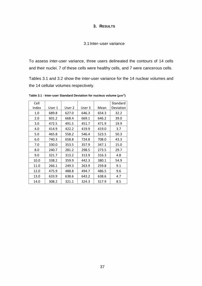
3.1 Inter–user variance

To assess inter-user variance, three users delineated the contours of 14 cells

and their nuclei. 7 of these cells were healthy cells, and 7 were cancerous cells.

Tables 3.1 and 3.2 show the inter-user variance for the 14 nuclear volumes and

the 14 cellular volumes respectively.

Table 3.1 - Inter-user Standard Deviation for nucleus volume ( )

Cell Index User 1 User 2 User 3 Mean

Standard Deviation

1.0 689.8 627.0 646.3 654.3 32.2

2.0 601.2 668.4 669.1 646.2 39.0

3.0 472.5 491.5 451.7 471.9 19.9

4.0 414.9 422.2 419.9 419.0 3.7

5.0 465.8 558.2 546.4 523.5 50.3

6.0 740.3 658.8 724.8 708.0 43.3

7.0 330.0 353.5 357.9 347.1 15.0

8.0 240.7 281.2 298.5 273.5 29.7

9.0 321.7 313.2 313.9 316.3 4.8

10.0 338.2 359.9 442.3 380.1 54.9

11.0 266.1 249.3 263.9 259.8 9.1

12.0 475.9 488.8 494.7 486.5 9.6

13.0 633.9 638.6 643.2 638.6 4.7

14.0 308.2 321.1 324.3 317.9 8.5

38

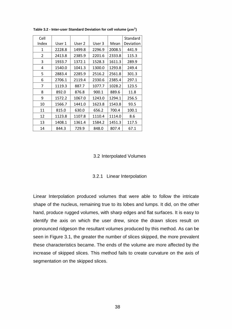
Table 3.2 - Inter-user Standard Deviation for cell volume ( )

Cell Index User 1 User 2 User 3 Mean

Standard Deviation

1 2228.8 1499.8 2296.9 2008.5 441.9

2 2413.8 2385.9 2201.6 2333.8 115.3

3 1933.7 1372.1 1528.3 1611.3 289.9

4 1540.0 1041.3 1300.0 1293.8 249.4

5 2883.4 2285.9 2516.2 2561.8 301.3

6 2706.1 2119.4 2330.6 2385.4 297.1

7 1119.3 887.7 1077.7 1028.2 123.5

8 892.0 876.8 900.1 889.6 11.8

9 1572.2 1067.0 1243.0 1294.1 256.5

10 1566.7 1441.0 1623.8 1543.8 93.5

11 815.0 630.0 656.2 700.4 100.1

12 1123.8 1107.8 1110.4 1114.0 8.6

13 1408.1 1361.4 1584.2 1451.3 117.5

14 844.3 729.9 848.0 807.4 67.1

3.2 Interpolated Volumes

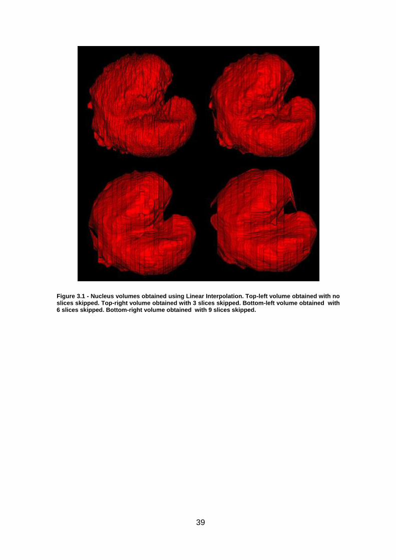
3.2.1 Linear Interpolation

Linear Interpolation produced volumes that were able to follow the intricate

shape of the nucleus, remaining true to its lobes and lumps. It did, on the other

hand, produce rugged volumes, with sharp edges and flat surfaces. It is easy to

identify the axis on which the user drew, since the drawn slices result on

pronounced ridgeson the resultant volumes produced by this method. As can be

seen in Figure 3.1, the greater the number of slices skipped, the more prevalent

these characteristics became. The ends of the volume are more affected by the

increase of skipped slices. This method fails to create curvature on the axis of

segmentation on the skipped slices.

39

Figure 3.1 - Nucleus volumes obtained using Linear Interpolation. Top-left volume obtained with no slices skipped. Top-right volume obtained with 3 slices skipped. Bottom-left volume obtained with 6 slices skipped. Bottom-right volume obtained with 9 slices skipped.

40

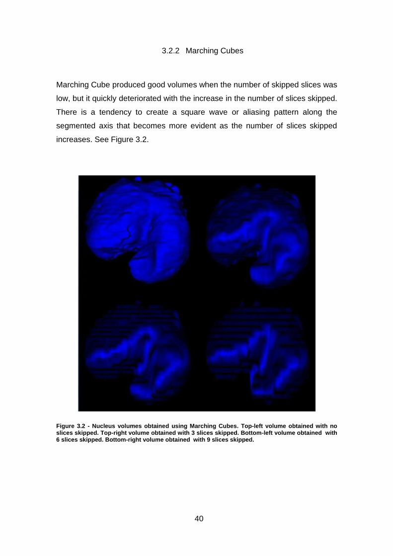
3.2.2 Marching Cubes

Marching Cube produced good volumes when the number of skipped slices was

low, but it quickly deteriorated with the increase in the number of slices skipped.

There is a tendency to create a square wave or aliasing pattern along the

segmented axis that becomes more evident as the number of slices skipped

increases. See Figure 3.2.

Figure 3.2 - Nucleus volumes obtained using Marching Cubes. Top-left volume obtained with no slices skipped. Top-right volume obtained with 3 slices skipped. Bottom-left volume obtained with 6 slices skipped. Bottom-right volume obtained with 9 slices skipped.

41

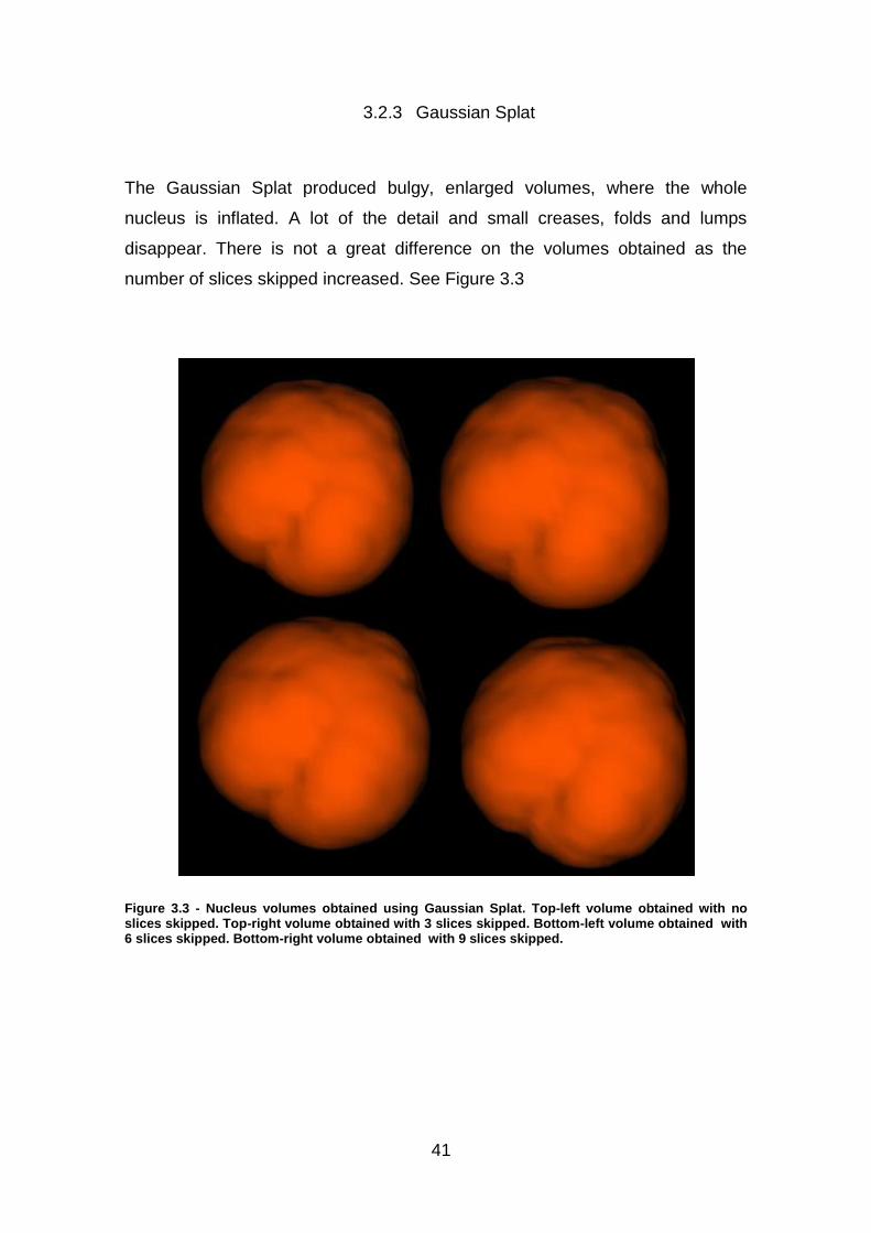
3.2.3 Gaussian Splat

The Gaussian Splat produced bulgy, enlarged volumes, where the whole

nucleus is inflated. A lot of the detail and small creases, folds and lumps

disappear. There is not a great difference on the volumes obtained as the

number of slices skipped increased. See Figure 3.3

Figure 3.3 - Nucleus volumes obtained using Gaussian Splat. Top-left volume obtained with no slices skipped. Top-right volume obtained with 3 slices skipped. Bottom-left volume obtained with 6 slices skipped. Bottom-right volume obtained with 9 slices skipped.

42

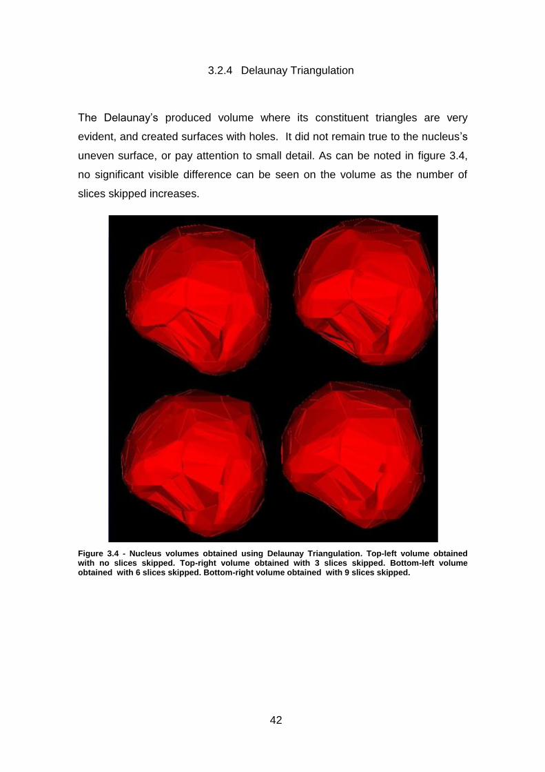
3.2.4 Delaunay Triangulation

The Delaunay’s produced volume where its constituent triangles are very

evident, and created surfaces with holes. It did not remain true to the nucleus’s

uneven surface, or pay attention to small detail. As can be noted in figure 3.4,

no significant visible difference can be seen on the volume as the number of

slices skipped increases.

Figure 3.4 - Nucleus volumes obtained using Delaunay Triangulation. Top-left volume obtained with no slices skipped. Top-right volume obtained with 3 slices skipped. Bottom-left volume obtained with 6 slices skipped. Bottom-right volume obtained with 9 slices skipped.

43

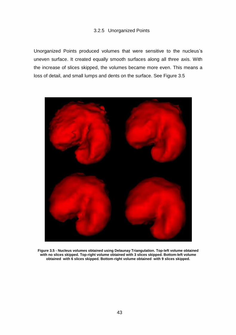
3.2.5 Unorganized Points

Unorganized Points produced volumes that were sensitive to the nucleus’s

uneven surface. It created equally smooth surfaces along all three axis. With

the increase of slices skipped, the volumes became more even. This means a

loss of detail, and small lumps and dents on the surface. See Figure 3.5

Figure 3.5 - Nucleus volumes obtained using Delaunay Triangulation. Top-left volume obtained with no slices skipped. Top-right volume obtained with 3 slices skipped. Bottom-left volume

obtained with 6 slices skipped. Bottom-right volume obtained with 9 slices skipped.

47

4. DISCUSSION

4.1 Software’s Inter-user variability

This technique of ground truth establishment has a high inter-user variance.

There are several parameters that can influence this. The users all had the

freedom to adjust the brightness and contrast to their liking. This can affect the

way the user observes less well defined boundaries. The users could also pick

the slices on which they drew or skipped, and the interpolation method was

used to define the contour on the skipped slices. Depending on how differently

the chosen slices were, the final volumes could reflect these choices. The users

also experiences fatigue, which makes the user more prone to error. Poor

judgment and human error must be considered as well. There might not always

be agreement on where the boundary is. Having trained experts trace the

volume could minimize these problems.

The inter-user variability for the cell was considerably greater than for the

nucleus. This could be explained by the higher contrast imparted by the

hematoxylin to the nucleus.

4.2 Interpolation Algorithms

To evaluate the performance of each interpolation algorithms we will use the

metrics described in section 2.4.

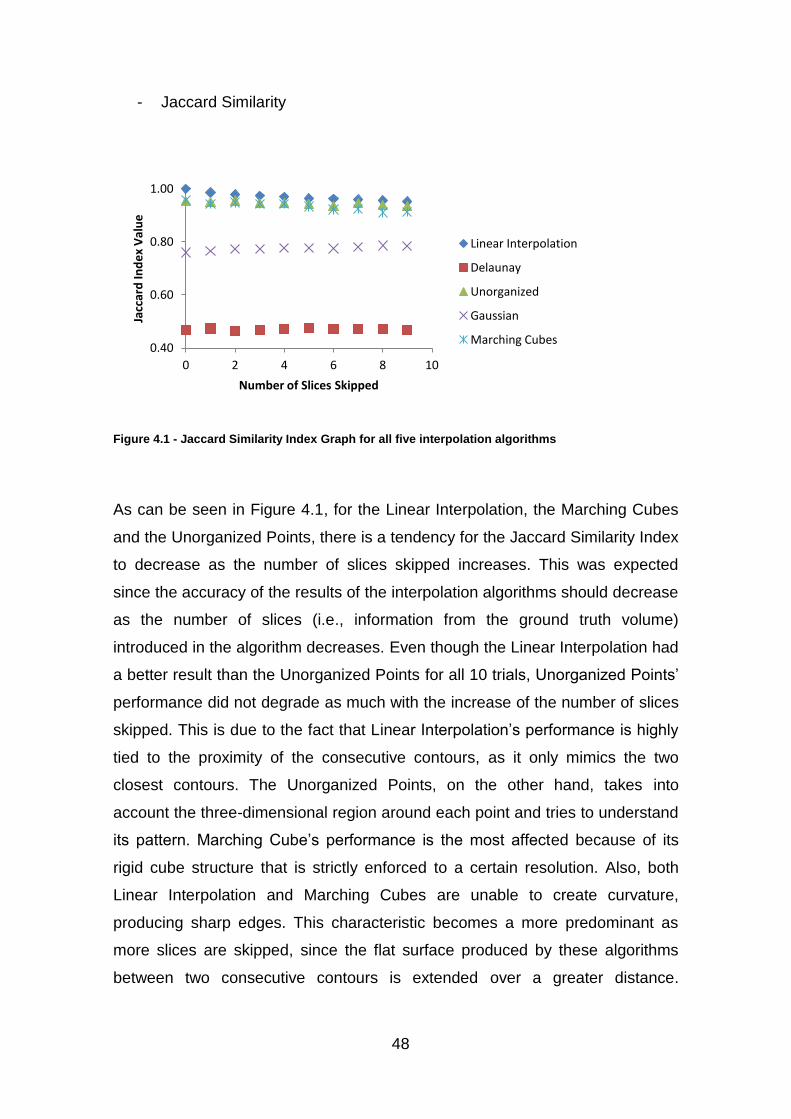
48

- Jaccard Similarity

Figure 4.1 - Jaccard Similarity Index Graph for all five interpolation algorithms

As can be seen in Figure 4.1, for the Linear Interpolation, the Marching Cubes

and the Unorganized Points, there is a tendency for the Jaccard Similarity Index

to decrease as the number of slices skipped increases. This was expected

since the accuracy of the results of the interpolation algorithms should decrease

as the number of slices (i.e., information from the ground truth volume)

introduced in the algorithm decreases. Even though the Linear Interpolation had

a better result than the Unorganized Points for all 10 trials, Unorganized Points’

performance did not degrade as much with the increase of the number of slices

skipped. This is due to the fact that Linear Interpolation’s performance is highly

tied to the proximity of the consecutive contours, as it only mimics the two

closest contours. The Unorganized Points, on the other hand, takes into

account the three-dimensional region around each point and tries to understand

its pattern. Marching Cube’s performance is the most affected because of its

rigid cube structure that is strictly enforced to a certain resolution. Also, both

Linear Interpolation and Marching Cubes are unable to create curvature,

producing sharp edges. This characteristic becomes a more predominant as

more slices are skipped, since the flat surface produced by these algorithms

between two consecutive contours is extended over a greater distance.

0.40

0.60

0.80

1.00

0 2 4 6 8 10

Jacc

ard

Ind

ex

Val

ue

Number of Slices Skipped

Linear Interpolation

Delaunay

Unorganized

Gaussian

Marching Cubes

49

Unorganized Points does not have this problem, seeing as it describes the

surface more organically, generating a smooth descriptive surface.

The Gaussian Splat and the Delaunay did not show the same tendency as the

other three methods. For the Gaussian Splat, the Jaccard Similarity Index

actually increases as the number of slices skipped increases. This can be

explained by the fact that the Gaussian Splat enlarges the volume of the cell. It

computes the volume creating a Gaussian distribution around each point that is

inputted into the algorithm, enlarging the volume of that point. The more points

that are introduced into the algorithm the greater the effect of that enlargement

will be. So the Gaussian Splat actually creates a volume closer to the size of the

ground truth volume when there is less slices introduced into the algorithm.

As for the Delaunay, it seems that the Jaccard Similarity Index remains

constant. This is because the Delaunay failed to create full surfaces, creating

volumes with holes. These holes were constant throughout all the volumes,

regardless of the number of slices skipped. Delaunay’s poor performance is

tied to the nature of our data and its highly uneven concentration of points.

For the Linear Interpolation, the Jaccard Similarity Index is 1 when the number

of slices skipped is zero. The reason for this is that this method only computes

the missing slices. When no slices are skipped, it just outputs exactly the same

information that was inputted into the algorithm. In the case of zero slices

skipped, the information that is introduced into the interpolation methods is the

ground truth volume; therefore the Linear Interpolation outputs the ground truth

volume.

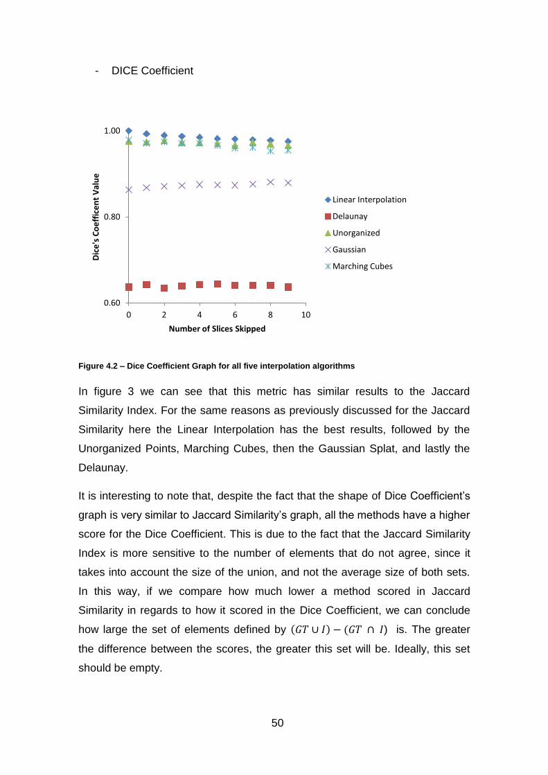
50

- DICE Coefficient

Figure 4.2 – Dice Coefficient Graph for all five interpolation algorithms

In figure 3 we can see that this metric has similar results to the Jaccard

Similarity Index. For the same reasons as previously discussed for the Jaccard

Similarity here the Linear Interpolation has the best results, followed by the

Unorganized Points, Marching Cubes, then the Gaussian Splat, and lastly the

Delaunay.

It is interesting to note that, despite the fact that the shape of Dice Coefficient’s

graph is very similar to Jaccard Similarity’s graph, all the methods have a higher

score for the Dice Coefficient. This is due to the fact that the Jaccard Similarity

Index is more sensitive to the number of elements that do not agree, since it

takes into account the size of the union, and not the average size of both sets.

In this way, if we compare how much lower a method scored in Jaccard

Similarity in regards to how it scored in the Dice Coefficient, we can conclude

how large the set of elements defined by ) is. The greater

the difference between the scores, the greater this set will be. Ideally, this set

should be empty.

0.60

0.80

1.00

0 2 4 6 8 10

Dic

e's

Co

eff

ice

nt

Val

ue



Delaunay

Unorganized

Gaussian

Marching Cubes

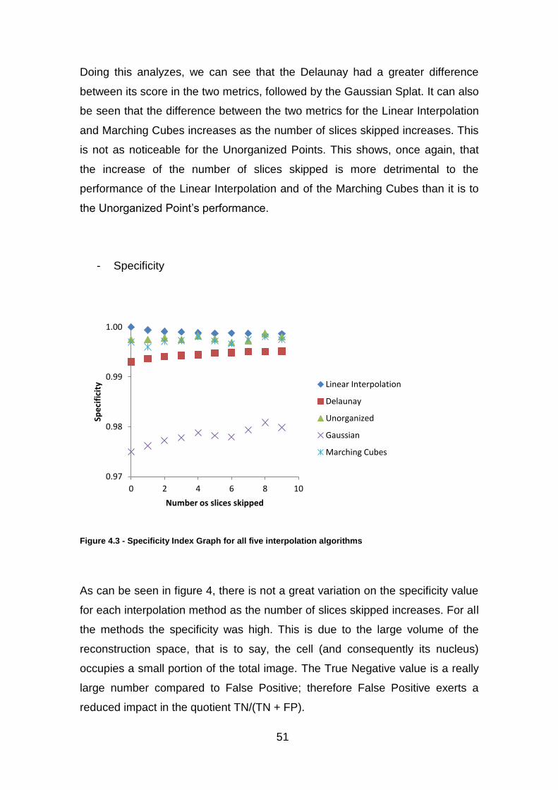
51

Doing this analyzes, we can see that the Delaunay had a greater difference

between its score in the two metrics, followed by the Gaussian Splat. It can also

be seen that the difference between the two metrics for the Linear Interpolation

and Marching Cubes increases as the number of slices skipped increases. This

is not as noticeable for the Unorganized Points. This shows, once again, that

the increase of the number of slices skipped is more detrimental to the

performance of the Linear Interpolation and of the Marching Cubes than it is to

the Unorganized Point’s performance.

- Specificity

Figure 4.3 - Specificity Index Graph for all five interpolation algorithms

As can be seen in figure 4, there is not a great variation on the specificity value

for each interpolation method as the number of slices skipped increases. For all

the methods the specificity was high. This is due to the large volume of the

reconstruction space, that is to say, the cell (and consequently its nucleus)

occupies a small portion of the total image. The True Negative value is a really

large number compared to False Positive; therefore False Positive exerts a

reduced impact in the quotient TN/(TN + FP).

0.97

0.98

0.99

1.00

0 2 4 6 8 10

Spe

cifi

city

Number os slices skipped


Delaunay

Unorganized

Gaussian

Marching Cubes

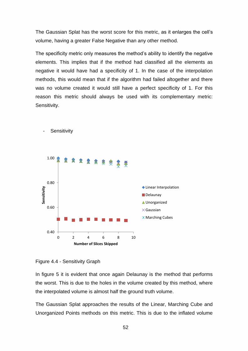
52

The Gaussian Splat has the worst score for this metric, as it enlarges the cell’s

volume, having a greater False Negative than any other method.

The specificity metric only measures the method’s ability to identify the negative

elements. This implies that if the method had classified all the elements as

negative it would have had a specificity of 1. In the case of the interpolation

methods, this would mean that if the algorithm had failed altogether and there

was no volume created it would still have a perfect specificity of 1. For this

reason this metric should always be used with its complementary metric:

Sensitivity.

- Sensitivity

Figure 4.4 - Sensitivity Graph

In figure 5 it is evident that once again Delaunay is the method that performs

the worst. This is due to the holes in the volume created by this method, where

the interpolated volume is almost half the ground truth volume.

The Gaussian Splat approaches the results of the Linear, Marching Cube and

Unorganized Points methods on this metric. This is due to the inflated volume

0.40

0.60

0.80

1.00

0 2 4 6 8 10

Sen

siti

vity



Delaunay

Unorganized

Gaussian

Marching Cubes

53

that the Gaussian Splat produces. Consequently, not many cell voxels are left

out of the Gaussian interpolated volume. As the sensitivity metric only takes into

account the ability to recognize positive elements, the Gaussian Splat’s score is

not hurt by including non-cell voxels within its interpolated volume. For this

reason, the sensitivity metric should also only be used with the specificity

metric.

The Linear Interpolation was the most sensitive method, followed by

Unorganized Points, the Gaussian Splat and the Marching Cubes. All these

methods had close values of sensitivity.

For all four metrics, the Linear Interpolation produced the best results. This can

be explained by the fact that due to its simplicity, it will have a stable

performance with various types of intricate data. It can be noted that, visually,

Unorganized Points produced a better volume as it generates smoother

surfaces, as opposed to the sharper edges and the flatter surfaces created by

the Linear Interpolation.

It is also interesting to note that the variance produced by Linear

Interpolation, Marching Cubes, and Unorganized Points, was not as significant

as the inter-user variance. In this way, the interpolation method minimizes the

human error.

55

5. CONCLUSION

We successfully designed a software program, the Ground Truth Evaluation,

which permits establishment of volumetric ground truth for segmentation of cell

CT images using interpolation. The interactive software interface allows the

user to record and archive tracings of cell components drawn with a stylus on a

tablet display showing an image of the cell, making it possible to convert the

results from human visual segmentation to a digital form.

Due to the fact that tracing the contour of desired cell components on all the

slices derived from the cell CT 3D image was very time consuming and tedious,

error was introduced to the manual tracing process from user fatigue. To speed

up the process and reduce the uncertainty and error introduced into the process

from this fatigue, the authors developed a software code to implement the use

of interpolation algorithms to reduce the number of slices that needed to be

traced manually. We investigated five different interpolation algorithms to

identify the one that produces the optimally segmented volume. The

interpolation algorithms studied included the following: Linear Interpolation,

Marching Cubes, Gaussian Splat, Delaunay Triangulation, and Unorganized

Points.

Results from the study showed that the Gaussian splat interpolation technique

tends to enlarge the volume. The Delaunay algorithm had trouble creating full

surfaces given the uneven density of the measured data. The Unorganized

Points algorithm produced good results, but it was both less sensitive and less

specific than the Linear Interpolation. Although the Marching Cubes algorithm

and the Linear Interpolation both showed a tendency to create sharper edges

than existed in the actual volume, this effect was more accentuated for the

Marching Cube algorithm.

To evaluate the performance of each interpolation algorithm the following

statistical metrics were used: Jaccard Similarity, Dice Coefficient, Specificity

and Sensitivity. After analyzing the results of each metric applied to the results

56

from each interpolation method independently, we concluded that Linear

Interpolation was the most accurate interpolation method, having had the most

optimal value compared to the actual volume for all four metrics.

Using Linear Interpolation, it is possible to speed up ground truth determination,

making the process of ground truth determination more

efficient. Our work provides a method to obtain ground truth for 3D cellular

image segmentation as well as many other medical segmentation problems.

With ground truth achieved, it is possible to validate 3D segmentation

algorithms. This is crucial to provide a documented methodology for future

research to improve and advance the field of quantitative 3D image analysis for

precise 3D cytopathological assessment of cells.

This method of ground truth establishment can also be used for other types of

medical images. Volumes with a more uniform surface, e.g. a bone, may benefit

even more from interpolation methods.

There are several aspects of the software that could be further explored and

improved in future work. Techniques to minimize human error could be studied

and developed, which include the combining of tracings from many people, intra

and inter user variability could be further studied, semi-automatic contour

generation, intelligent thresholding and other related research. For that purpose,

a digital phantom could be used to study the error associated with tracing and to

optimize tracing techniques. Other interpolation algorithms could also be

explored, as well as the possibility of combining and optimizing current

algorithms.

57

BIBLIOGRAPHY

[1] R. Siegel, D. Naishadham, and A. Jemal, “Cancer statistics, 2012,” CA: a cancer

journal for clinicians, 2012.

[2] J. Nickerson, “Nuclear dreams: the malignant alteration of nuclear architecture,”

Journal of cellular biochemistry, vol. 70, no. 2, pp. 172 – 180, 1998.

[3] D. Zink, A. H. Fischer, and J. A. Nickerson, “Nuclear structure in cancer cells,”

Nat Rev Cancer, vol. 4, no. 9, pp. 677–687, Sep. 2004.

[4] M. Fauver, E. Seibel, J. Rahn, M. Meyer, F. Patten, T. Neumann, and A. Nelson,

“Three-dimensional imaging of single isolated cell nuclei using optical projection

tomography,” Optics Express, vol. 13, no. 11, pp. 4210–4223, 2005.

[5] Q. Miao, J. R. Rahn, E. J. Seibel, A. Tourovskaia, M. G. Meyer, T. Neumann,

and A. C. Nelson, “Dual-modal three-dimensional imaging of single cells with

isometric high resolution using an optical projection tomography microscope,” J.

Biomed. Opt, vol. 14, no. 6, pp. 064035–064035–6, 2009.

[6] V. Nandakumar, L. Kelbauskas, K. F. Hernandez, K. M. Lintecum, P. Senechal,

K. J. Bussey, P. C. W. Davies, R. H. Johnson, and D. R. Meldrum, “Isotropic 3D

Nuclear Morphometry of Normal, Fibrocystic and Malignant Breast Epithelial Cells

Reveals New Structural Alterations,” PLoS ONE, vol. 7, no. 1, p. e29230, Jan.

2012.

[7] V. Nandakumar, L. Kelbauskas, R. Johnson, and D. Meldrum, “Quantitative

characterization of preneoplastic progression using single-cell computed

tomography and three-dimensional karyometry,” Cytometry Part A, vol. 79A, no. 1,

pp. 25–34, 2011.

[8] V. Nandakumar, K. Hernandez, Beatriz Rodolpho, “Quantitative assessment of

3D nuclear architecture in colon epithelial cells by micro-optical computed

tomography,” presented at the AACR, 2012.

[9] V. Nandakumar,R. H. Johnson, “A physical sciences network characterization of

non-tumorigenic and metastatic cells,” Scientific Reports, vol. 3, Apr. 2013.

[10] Vivek Nandakumar, “Three-dimensional morphological biosignatures for cancer

by automated analysis of transmission-mode optical cell CT images,” Arizona State

University, 2013.

[11] M. G. Meyer, M. Fauver, J. R. Rahn, T. Neumann, F. W. Patten, E. J. Seibel,

and A. C. Nelson, “Automated cell analysis in 2D and 3D: A comparative study,”

Pattern Recognition, vol. 42, no. 1, pp. 141–146, Jan. 2009.

[12] M. Fauver, E. Seibel, J. Rahn, M. Meyer, F. Patten, T. Neumann, and A. Nelson,

“Three-dimensional imaging of single isolated cell nuclei using optical projection

tomography,” Optics Express, vol. 13, no. 11, pp. 4210–4223, 2005.

[13] Q. Miao, A. P. Reeves, F. W. Patten, and E. J. Seibel, “Multimodal 3D Imaging

of Cells and Tissue, Bridging the Gap Between Clinical and Research Microscopy,”

Ann Biomed Eng, vol. 40, no. 2, pp. 263–276, Feb. 2012.

[14] D. J. Withey and Z. J. Koles, “Medical Image Segmentation: Methods and

Software,” in Joint Meeting of the 6th International Symposium on Noninvasive

58

Functional Source Imaging of the Brain and Heart and the International

Conference on Functional Biomedical Imaging, 2007. NFSI-ICFBI 2007, 2007, pp.

140–143.

[15] P. L. Rosin, “Unimodal thresholding,” Pattern Recognition, vol. 34, no. 11, pp.

2083–2096, Nov. 2001.

[16] N. Otsu, “A threshold selection method from gray-level histograms,”

AUTOMATICA (OXF), vol. 11, no. 285–296, p. 23, 1975.

[17] M. Xu and P. Franti, “A heuristic K-means clustering algorithm by kernel PCA,”

in 2004 International Conference on Image Processing, 2004. ICIP ’04, 2004, vol.

5, pp. 3503–3506 Vol. 5.

[18] T. Kanungo, D. M. Mount, N. S. Netanyahu, C. D. Piatko, R. Silverman, and A.

Y. Wu, “An efficient k-means clustering algorithm: analysis and implementation,”

IEEE Transactions on Pattern Analysis and Machine Intelligence, vol. 24, no. 7, pp.

881–892, 2002.

[19] “TurtleSeg,” TurtleSeg. [Online]. Available: http://www.turtleseg.org/.

[20] “ITK-SNAP,” ITK-SNAP. [Online]. Available: http://www.itksnap.org.

[21] “3D-DOCTOR,” 3D-DOCTOR, medical modeling, 3D medical imaging. .

[22] J. Y. Chen, F. J. Seagull, P. Nagy, P. Lakhani, E. R. Melhem, E. L. Siegel, and

N. M. Safdar, “Computer Input Devices: Neutral Party or Source of Significant

Error in Manual Lesion Segmentation?,” J Digit Imaging, vol. 24, no. 1, pp. 135–

141, Feb. 2011.

[23] Ferreira, P. M., T. Mendonça, P. Rocha, and J. Rozeira., “A new interface for

manual segmentation of dermoscopic images,” VipIMAGE, pp. 12–14, 2011.

[24] F. Salaffi, M. Carotti, A. Ciapetti, A. Ariani, S. Gasparini, and W. Grassi,

“Validity of a computer-assisted manual segmentation software to quantify wrist

erosion volume using computed tomography scans in rheumatoid arthritis,” BMC

Musculoskeletal Disorders, vol. 14, no. 1, p. 265, Sep. 2013.

[25] A. H. Fischer, K. A. Jacobson, J. Rose, and R. Zeller, “Hematoxylin and Eosin

Staining of Tissue and Cell Sections,” Cold Spring Harb Protoc, vol. 2008, no. 5, p.

pdb.prot4986, May 2008.

[26] “Microsoft .NET.” [Online]. Available: http://www.microsoft.com/net.

[27] “VTK.” [Online]. Available: http://www.vtk.org.

[28] W. E. Lorensen and H. E. Cline, “Marching cubes: A high resolution 3D surface

construction algorithm,” SIGGRAPH Comput. Graph., vol. 21, no. 4, pp. 163–169,

Aug. 1987.

[29] Zwicker, Matthias, Jussi Räsänen, Mario Botsch, Carsten Dachsbacher, and

Mark Pauly, “Perspective Accurate Splatting,” Graphics interface, vol. 2004, pp.

247–254.

[30] J. R. Shewchuk, “Delaunay refinement algorithms for triangular mesh

generation,” Computational Geometry, vol. 22, no. 1–3, pp. 21–74, May 2002.

[31] H. Hoppe, T. DeRose, T. Duchamp, J. McDonald, and W. Stuetzle, “Surface

reconstruction from unorganized points,” SIGGRAPH Comput. Graph., vol. 26, no.

2, pp. 71–78, Jul. 1992.

[32] P. Jaccard, “The Distribution of the Flora in the Alpine Zone.1,” New

Phytologist, vol. 11, no. 2, pp. 37–50, 1912.

[33] L. R. Dice, “Measures of the Amount of Ecologic Association Between

Species,” Ecology, vol. 26, no. 3, p. 297, Jul. 1945.

[34] K. H. Zou, S. K. Warfield, A. Bharatha, C. M. C. Tempany, M. R. Kaus, S. J.

Haker, W. M. Wells III, F. A. Jolesz, and R. Kikinis, “Statistical validation of image

59

segmentation quality based on a spatial overlap index1: scientific reports,”

Academic Radiology, vol. 11, no. 2, pp. 178–189, Feb. 2004.

61

APPENDIX A:

PSEUDO CODE FOR THE LINEAR INTERPOLATION AND

MARCHING CUBES ALGORITHMS

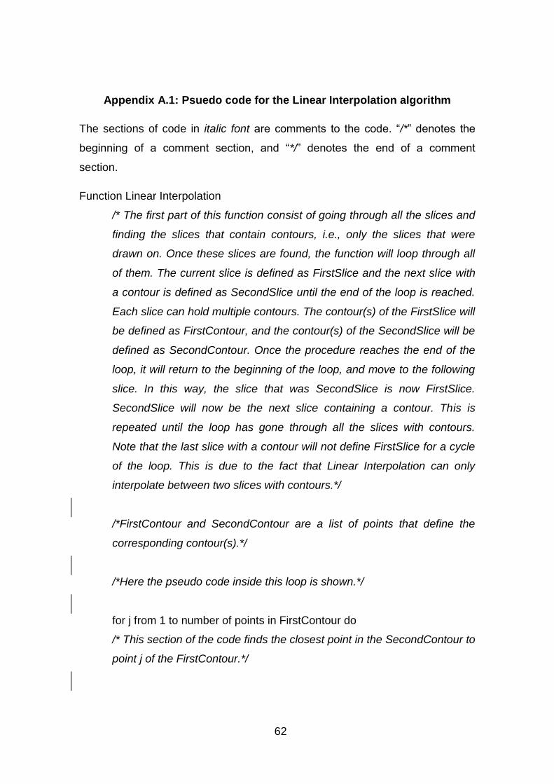
62

Appendix A.1: Psuedo code for the Linear Interpolation algorithm

The sections of code in italic font are comments to the code. “/*” denotes the

beginning of a comment section, and “*/” denotes the end of a comment

section.

Function Linear Interpolation

/* The first part of this function consist of going through all the slices and

finding the slices that contain contours, i.e., only the slices that were

drawn on. Once these slices are found, the function will loop through all

of them. The current slice is defined as FirstSlice and the next slice with

a contour is defined as SecondSlice until the end of the loop is reached.

Each slice can hold multiple contours. The contour(s) of the FirstSlice will

be defined as FirstContour, and the contour(s) of the SecondSlice will be

defined as SecondContour. Once the procedure reaches the end of the

loop, it will return to the beginning of the loop, and move to the following

slice. In this way, the slice that was SecondSlice is now FirstSlice.

SecondSlice will now be the next slice containing a contour. This is

repeated until the loop has gone through all the slices with contours.

Note that the last slice with a contour will not define FirstSlice for a cycle

of the loop. This is due to the fact that Linear Interpolation can only

interpolate between two slices with contours.*/

/*FirstContour and SecondContour are a list of points that define the

corresponding contour(s).*/

/*Here the pseudo code inside this loop is shown.*/

for j from 1 to number of points in FirstContour do

/* This section of the code finds the closest point in the SecondContour to

point j of the FirstContour.*/

63

/* Define the variable minDistance, which will define the minimum

distance found between point j and a point in the SecondContour,

as the distance between point j and the first point of the

SecondContour. This distance is calculated using the formula:

*/

minDistance = sqrt((FirstContour[j].X - SecondContour[0].X) *

(FirstContour[j].X - SecondContour[0].X) + (FirstContour[j].Y -

SecondContour[0].Y) * (FirstContour[j].Y - SecondContour[0].Y))

/* Define the variable closestPoint, which will contain the point in

the SecondContour whose distance to point j is minimum, as the

first point of SecondContour.*/

closestPoint = SecondContour[0]

/*Loop through all the points of the SecondContour */

for k from 1 to the length of SecondContour do

/* Calculate the distance of the current point in Second

Contour to point j */

currentDistance =sqrt((FirstContour[j].X -

SecondContour[k].X) * (FirstContour[j].X -

SecondContour[k].X) + (FirstContour[j].Y -

SecondContour[k].Y) * (FirstContour[j].Y -

SecondContour[k].Y))

/*Check if the distance of current point k is smaller than the

minDistance. If it is update the variable minDistance with

the value currentDistance, and the variable closestPoint to

be point k.*/

if the currentDistance is smaller than minDistance do

minDistance = currentDistance

closestPoint = SecondContour[k]

end if

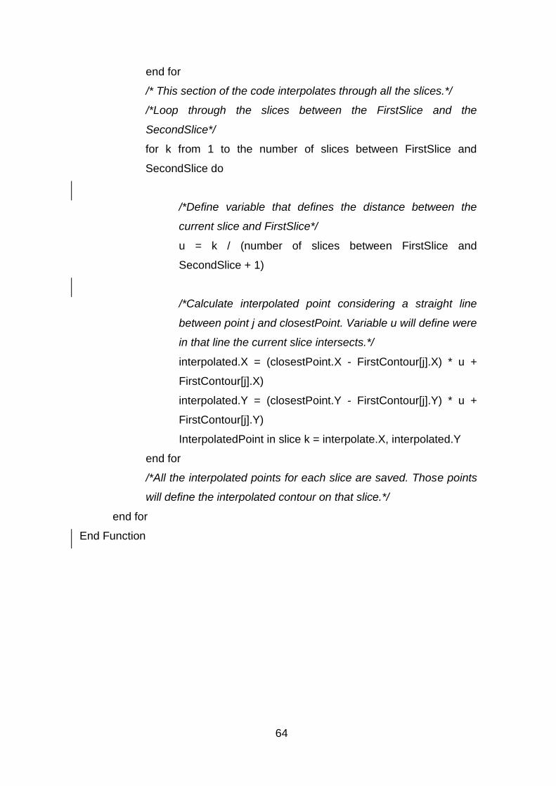
64

end for

/* This section of the code interpolates through all the slices.*/

/*Loop through the slices between the FirstSlice and the

SecondSlice*/

for k from 1 to the number of slices between FirstSlice and

SecondSlice do

/*Define variable that defines the distance between the

current slice and FirstSlice*/

u = k / (number of slices between FirstSlice and

SecondSlice + 1)

/*Calculate interpolated point considering a straight line

between point j and closestPoint. Variable u will define were

in that line the current slice intersects.*/

interpolated.X = (closestPoint.X - FirstContour[j].X) * u +

FirstContour[j].X)

interpolated.Y = (closestPoint.Y - FirstContour[j].Y) * u +

FirstContour[j].Y)

InterpolatedPoint in slice k = interpolate.X, interpolated.Y

end for

/*All the interpolated points for each slice are saved. Those points

will define the interpolated contour on that slice.*/

end for

End Function

65

Appendix A.2: Psuedo code for the Marching Cubes algorithm

The sections of code in italic font are comments to the code. “/*” denotes the

beginning of a comment section, and “*/” denotes the end of a comment

section.

Marching Cubes Function

/*The slices with contours are loaded into the Marching Cubes in a 3D

Matrix. The function will return the triangles that define the surface.*/

/*Create a list of Triangles */

ListOfTriangles

/*Loop through the cells of the matrix to create cubes*/

for i from 1 to the number of rows of Matrix -1

for j from 1 to the number of columns of Matrix -1

for k to the number of slices in the Matrix -1

/*Create cube, a variable that holds 8 vertices and their

corresponding X, Y and Z coordinates, as well as each vertex’s

value*/

Create cube and define all 8 vertices by their location and the

matrix value at that point

/*Define each vertex of the cube*/

cubeVertex[0].X = i

cubeVertex[0].Y = j

cubeVertex[0].Z = k

cubeVertexValue[0] = Matrix[i, j, k]

/*repeat the above for each corner of the cube */

66

/*Once a cube is created it is possible to calculate the triangular facets

required to represent the isosurface in the cube. */

/*Define variable cubeindex, which tells us which vertices are inside of

the surface, as zero. This index will determine the triangle(s) that

characterize the surface inside the corresponding cube */

cubeindex = 0

/* Determine the value of cubeindex for this cube taking into account the

isolevel defined by the user. */

if cubeVertexValue[0] < isolevel then do

assign the first bit of cubeindex to 1


assign the second bit of cubeindex to 1


assign the third bit of cubeindex to 1


assign the forth bit of cubeindex to 1


assign the fifth bit of cubeindex to 1


assign the sixth bit of cubeindex to 1


assign the seventh bit of cubeindex to 1


assign the eighth bit of cubeindex to 1

/* Cube is entirely in/out of the surface, which means there will be no

triangles inside it */

if all of cubeindex’s bits are 0 end cycle for this cube

/* Find the vertices where the surface intersects the cube */

/* This is done with the help of the functions VertexInterp and edgeTable.

VertexInterp linearly interpolates the position where an isosurface cuts an

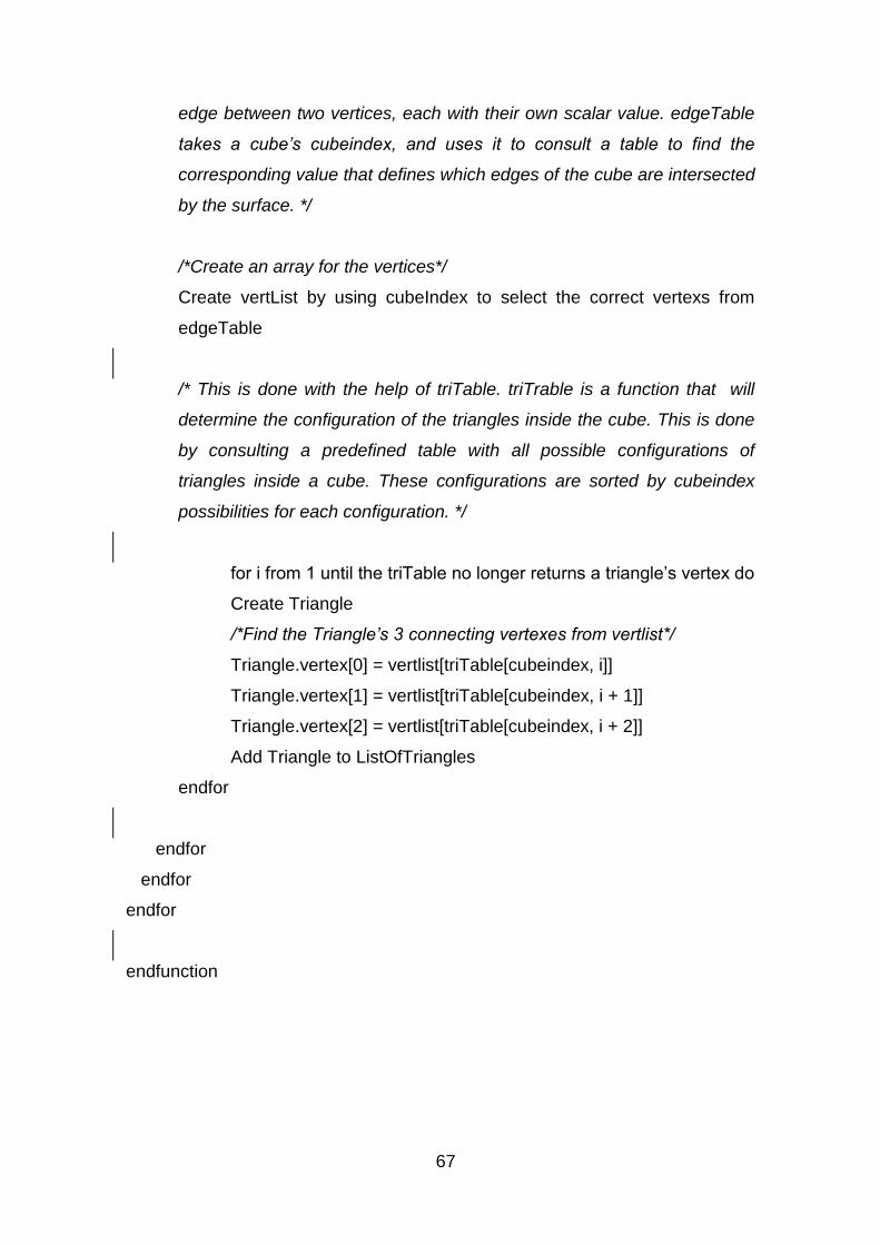
67

edge between two vertices, each with their own scalar value. edgeTable

takes a cube’s cubeindex, and uses it to consult a table to find the

corresponding value that defines which edges of the cube are intersected

by the surface. */

/*Create an array for the vertices*/

Create vertList by using cubeIndex to select the correct vertexs from

edgeTable

/* This is done with the help of triTable. triTrable is a function that will

determine the configuration of the triangles inside the cube. This is done

by consulting a predefined table with all possible configurations of

triangles inside a cube. These configurations are sorted by cubeindex

possibilities for each configuration. */

for i from 1 until the triTable no longer returns a triangle’s vertex do

Create Triangle

/*Find the Triangle’s 3 connecting vertexes from vertlist*/

Triangle.vertex[0] = vertlist[triTable[cubeindex, i]]

Triangle.vertex[1] = vertlist[triTable[cubeindex, i + 1]]

Triangle.vertex[2] = vertlist[triTable[cubeindex, i + 2]]

Add Triangle to ListOfTriangles

endfor

endfor

endfor

endfor

endfunction

ground truth determination for segmentation of tomographic ... · ground truth determination for...

Documents