feasibility test of the simulation of a running … · feasibility test of the simulation of a...
TRANSCRIPT
FEASIBILITY TEST OF THE SIMULATION
OF A RUNNING TURBINE WITH
OPENFOAM
DANIELA FIGUEIREDO GOMES DE OLIVEIRA
Dissertação submetida para satisfação parcial dos requisitos do grau de
MESTRE EM ENGENHARIA CIVIL — ESPECIALIZAÇÃO EM HIDRÁULICA
Orientador: Professor Doutor João Pedro Pêgo
Coorientador: Elena-Maria Klopries, M.Sc. RWTH
JULHO 2015

MESTRADO INTEGRADO EM ENGENHARIA CIVIL 2012/2013
DEPARTAMENTO DE ENGENHARIA CIVIL
Tel. +351-22-508 1901
Fax +351-22-508 1446
Editado por
FACULDADE DE ENGENHARIA DA UNIVERSIDADE DO PORTO
Rua Dr. Roberto Frias
4200-465 PORTO
Portugal
Tel. +351-22-508 1400
Fax +351-22-508 1440
http://www.fe.up.pt
Reproduções parciais deste documento serão autorizadas na condição que seja
mencionado o Autor e feita referência a Mestrado Integrado em Engenharia Civil -
2012/2013 - Departamento de Engenharia Civil, Faculdade de Engenharia da
Universidade do Porto, Porto, Portugal, 2013.
As opiniões e informações incluídas neste documento representam unicamente o
ponto de vista do respetivo Autor, não podendo o Editor aceitar qualquer
responsabilidade legal ou outra em relação a erros ou omissões que possam existir.
Este documento foi produzido a partir de versão eletrónica fornecida pelo respetivo
Autor.

Feasibility test of the simulation of a running turbine with OpenFOAM
To my Grandfather.
Knowing is not enough, we must apply. Willing is not enough, we must do.
Johann Wolfgang von Goethe

Feasibility test of the simulation of a running turbine with OpenFOAM

Feasibility test of the simulation of a running turbine with OpenFOAM
i
ACKNOWLEDGMENTS
First of all, to my scientific mentor and the person who contributed the most to this work, Elena
Klopries, M.Sc. RWTH. For all the never ending help, patience and teaching, a sincere thank you. It
was for me a privilege to have learned from you.
To Professor Dr. João Pedro Pêgo, for all the availability, since the first moment, to follow the
development of my dissertation. For contributing with wisdom and knowledge when most necessary.
To all the professors in the hydraulics department of the Faculty of Engineering of the University of
Porto. In the end of the year, I was certain I had chosen the right specialization.
To my friends and especially Marta Morais, for being always and unconditionally a source of
inspiration and encouragement in good times, but, above all, in overcoming times.
To Nuno Quelhas, my partner in this Erasmus experience. For his constant support and friendship a
heartfelt thanks.
To my grandparents, for their support, not only emotionally, but also financially. To my mother, for
being the engine of our home, for all the effort made so that this path and especially this dissertation
were possible to be performed under the conditions they were.
Finally to my brothers, Ricardo and João. That the pride they can feel in me could be equivalent to the
immensity they symbolize in my life.

Feasibility test of the simulation of a running turbine with OpenFOAM
ii
Feasibility test of the simulation of a running turbine with OpenFOAM
iii
AGRADECIMENTOS
Primeiramente à minha mentora científica e à pessoa que mais contribuiu para este trabalho, Elena
Klopries, M.Sc. RWTH. Por toda a interminável ajuda, pela paciência e por todo o conhecimento
transmitido, um sincero obrigado. Foi para mim um privilégio ter aprendido consigo.
Ao Professor Dr. João Pedro Pêgo, por toda a disponibilidade desde o primeiro momento para
acompanhar o desenvolvimento da minha tese. Por ter contribuído com sabedoria e conhecimento na
altura certa.
A todos os professores no departamento de hidráulica da Faculdade de Engenharia da Universidade do
Porto. No final do ano, eu estava certa de que tinha escolhido a especialização certa.
A todos os meus amigos, e em especial à Marta Morais, por serem sempre e incondicionalmente uma
fonte de inspiração e de incentivo quer nos bons momentos, quer, acima de tudo, nos momentos de
superação.
Ao Nuno Quelhas, meu companheiro desta experiência de Erasmus. Pelo seu constante apoio e
amizade, um agradecimento de coração.
Aos meus avós, pelo apoio não só emocional, como financeiro. À minha mãe por ser o motor do nosso
lar, por todo o esforço que fez para que este percurso e em especial esta dissertação fosse possível de
ser realizada nas condições que foi.
E por fim, aos meus irmãos, Ricardo e João. Que o orgulho que possam sentir em mim seja
equiparável à imensidão que simbolizam na minha vida.

Feasibility test of the simulation of a running turbine with OpenFOAM
iv
Feasibility testo f the simulation of a running turbine with OpenFOAM
v
ABSTRACT
Field and laboratory studies reviewing the passage of fish through hydroelectric turbines have been
object of research over the years. The biggest causes of fish mortality when passing a hydroelectric
turbine are described as being the variation of pressure, cavitation, shear stress as well as strike and
grinding. Most of the models used to calculate fish mortality are based on the probability of the injury
to happen depending on parameters like flow, length of the fish or the angle of the turbine’s vanes. But
most of these models are so-called black-box-models where the real, physical processes are not shown.
This is where computational fluid dynamics plays an important part. It is possible to model and
simulate different structures and in this way also the flow that may occur. Like this, it is possible to
model what happens to a fish when passing a turbine, showing the real processes that happens during
the passage.
In this work, a four blade propeller turbine is modelled with the software OpenFOAM - Open Field
Operation and Manipulation. The main focus of the work is on the simulation of the turbine’s
movement.
Two different approaches with regard to the simulation of the movement were made in order to better
comprehend which one could be more suitable and more economical with regard to the given
resources of the computers. The first one focused on an oscillating movement and the second one was
done with a rotational movement. Both were solved resorting to turbulent resolution model SST k-ω.
KEYWORDS: fish mortality, hydraulic turbines, Computational Fluid Dynamis, OpenFoam.

Feasibility test of the simulation of a running turbine with OpenFOAM
vi
Feasibility test of the simulation of a running turbine with OpenFOAM
vii
RESUMO
Ao longo do tempo, têm sido objeto de pesquisa estudos práticos e teóricos acerca da passagem de
peixes através de turbinas hidroelétricas. As maiores causas de mortalidade de peixes em turbinas
hidroelétricas são a variação de pressão, cavitação, tensão de cisalhamento, assim como colisões. A
maioria dos modelos utilizados para calcular a mortalidade de peixes são baseados na probabilidade de
as lesões acontecerem sob a dependência de parâmetros como o tipo de escoamento, comprimento do
peixe ou o ângulo das pás da turbina. No entanto, estes modelos são apelidados de “black box
models”, nos quais são negligenciados os processos físicos reais.
Perante estas situações revela-se importante o papel da dinâmica computacional de fluidos. É possível
modelar e simular diferentes estruturas e desta forma também o escoamento que pode ocorrer.
Portanto, é possível modelar o que acontece a um peixe durante a sua passagem por uma turbina,
sendo possível observar os processos que ocorrem durante essa passagem.
Neste trabalho, foi modelada uma turbina de quatro pás fazendo recurso do software OpenFOAM –
Open Field Operation and Manipulation. O trabalho está principalmente focado na simulação do
movimento de uma turbina.
Foram feitas duas abordagens diferentes em relação à simulação do movimento, de forma a que seja
possível compreender qual será a mais adequada e económica tendo em conta os recursos dos
computadores. A primeira abordagem está focada num movimento de oscilação e a segunda num
movimento de rotação. Ambas foram resolvidas fazendo recurso do modelo SST k-ω.
PALAVRAS-CHAVE: mortalidade de peixes, turbina hidráulica, dinâmica computacional de fluidos,
OpenFOAM

Feasibility test of the simulation of a running turbine with OpenFOAM
viii
Feasibility test of the simulation of a running turbine with OpenFOAM
ix
TABLE OF CONTENTS
ACKNOWLEDGMENTS.......................................................................................................................... i
AGRADECIMENTOS............................................................................................................................ iii
ABSTRACT .............................................................................................................................. v
RESUMO ........................................................................................................................................... vii
1. INTRODUCTION ......................................................................................................... 1
2. THEORETICAL FRAMEWORK REGARDING FISH PASSAGE THROUGH RUNNING TURBINES ......................................... 3
2.1. FISH MORTALITY ASSOCIATED WITH RUNNING TURBINES ........................................................... 3
2.2. CHARACTERISTICS OF RUNNING TURBINES ......................................................................... 3
2.3. SOURCES OF FISH MORTALITY ........................................................................................... 8
2.3.1. Pressure effect ....................................................................................................................... 9
2.3.2. Water turbulence and shearing currents ................................................................................ 10
2.3.3. Mechanical contact with blades ............................................................................................. 10
2.4 REVIEW ON STUDIES DONE REGARDING THE SOURCES OF FISH MORTALITY ......................... 10
2.4.1. Review on pressure studies .................................................................................................. 10
2.4.2. Review on water turbulence and shearing currents studies ................................................... 12
2.4.3. Review of mechanical studies ............................................................................................... 13
3. COMPUTATIONAL FLUID DYNAMICS - CFD ............................... 15
3.1. INTRODUCTION TO COMPUTATIONAL FLUID DYNAMICS............................................................. 15
3.2. SPECIAL FEATURES OF THE CFD TOOLS ................................................................................. 16
3.2.1. PRE-PROCESSOR....................................................................................................................... 16
3.2.2. SOLVER .................................................................................................................................... 17
3.2.3. POST-PROCESSOR ..................................................................................................................... 17
3.3. MESHES .................................................................................................................................... 19
3.4. MAIN PRINCIPLES ABOUT FLUID DYNAMICS .............................................................................. 21
3.4.1. MASS CONSERVATION – LAW OF CONTINUITY ................................................................................ 21
3.4.2. CONSERVATION OF THE MOMENTUM – SECOND LAW OF NEWTON..................................................... 23
3.4.3. CONSERVATION OF ENERGY IN A PARTICLE – FIRST LAW OF THERMODYNAMICS ................................. 24
Feasibility test of the simulation of a running turbine with OpenFOAM
x
3.5. TURBULENT FLOW .................................................................................................................... 25
3.6. TURBULENCE MODELS ............................................................................................................. 26
3.6.1. MODELS BASED ON REYNOLDS AVERAGED NAVIER-STOKES ........................................................... 26
2.6.1.1. Linear Eddy Viscosity Model ................................................................................................. 27
3.6.2. LARGE EDDY SIMULATION ........................................................................................................... 31
3.6.3. DIRECT NUMERICAL SIMULATION ................................................................................................. 32
3.7. PRINCIPLES OF SOLUTION OF THE GOVERNING EQUATIONS ..................................................... 33
3.7.1. FINITE DIFFERENCE METHOD ....................................................................................................... 35
3.7.2. FINITE VOLUME METHOD ............................................................................................................. 35
3.7.3. FINITE ELEMENT METHOD ............................................................................................................ 36
4. COMPUTATIONAL FLUID DYNAMICS - Procedure ............... 37
4.1. DESCRIPTION OF THE MODEL ................................................................................................... 37
4.2. PROCEDURE ............................................................................................................................. 37
4.3. SOFTWARE PROCEDURE - OPENFOAM ................................................................................... 38
4.4. GEOMETRY DEFINITION AND BOUNDARY CONDITIONS .............................................................. 40
4.5. MESH GENERATION .................................................................................................................. 42
4.6. NUMERICAL RESOLUTIONS MODELS ......................................................................................... 44
4.7. INITIAL CONDITIONS .................................................................................................................. 45
4.8. DEFINITION OF THE MOVEMENT OF THE TURBINE ..................................................................... 44
4.8.1. FIRST APPROACH RESORTING TO ANGULAROSCILLATINGVELOCITY .................................................. 45
4.8.2. SECOND APPROACH RESORTING TO ANGULARVELOCITY................................................................. 45
4.9. SOLUTION AND ALGORITHM CONTROL ..................................................................................... 52
4.10. DATA CONTROL ...................................................................................................................... 53
5. CONCLUSION AND FUTURE WORKS ................................................ 55
5.1. RESULTS OF STUDY .................................................................................................................. 55
5.2. FUTURE WORKS ........................................................................................................................ 57
BIBLIOGRAPHY ...................................................................................................................... 59
APPENDIX......................................................................................................................................... 63
Feasibility test of the simulation of a running turbine with OpenFOAM
xi
FIGURES INDEX
Fig.1 – Operating system of an Impulse Turbine .................................................................................. 4
Fig. 2 – Operating system of a Reaction Turbine ................................................................................. 5
Fig. 3 – Basic layout of a Kaplan turbine .............................................................................................. 6
Fig. 4 – Basic layout of a Francis turbine ............................................................................................. 7
Fig. 5 – Sources of injury to fish passing through hydropower turbines ................................................ 8
Fig. 6 – Pressure changes in a) Francis turbines and b) STRAFLO turbines ........................................ 9
Fig. 7 – Pressure exposure simulation of a turbine passage for surface and depth acclimated fish ..... 11
Fig. 8 – Flow around a cylinder: grid. ................................................................................................. 17
Fig. 9 – Velocity vectors regarding the flow around a cylinder. ........................................................... 18
Fig. 10 – Iso-surface of pressure regarding flow around a cylinder ..................................................... 18
Fig. 11 – Structured mesh ................................................................................................................. 19
Fig. 12 – Unstructured mesh ............................................................................................................. 19
Fig. 13 – Fluid element for conservation laws .................................................................................... 22
Fig. 14 – Mass flows in and out of fluid element ................................................................................. 22
Fig. 15 – Turbulence in a water jet..................................................................................................... 25
Fig. 16 – Structured mesh (or grid) in two dimensions – physical space ............................................. 33
Fig. 17 – Structured mesh (or grid) in two dimensions – computational space .................................... 34
Fig. 18 – Cell centred scheme ........................................................................................................... 35
Fig. 19 – Cell-vertex scheme ............................................................................................................. 36
Fig. 20 – Overview of OpenFOAM structure ...................................................................................... 38
Fig. 21 – Single block structure ......................................................................................................... 40
Fig. 22 – Block defined with blockMeshDict ....................................................................................... 41
Fig. 23 – .stl file of the turbine ........................................................................................................... 42
Fig. 24 – Part of the view of the turbine mesh .................................................................................... 43
Fig. 25 – Part of the view of the turbine mesh with the .stl file ............................................................ 44
Fig. 26 – Mechanism of Oscillating Velocity ....................................................................................... 46
Fig. 27 – Time step 1 corresponding to 0.01s .................................................................................... 49
Fig. 28 – Time step 15 corresponding to 0.015s ................................................................................ 49
Fig. 29 – Time step 100 corresponding to 1s ..................................................................................... 50
Fig. 30 – Time step 200 corresponding to 2s ..................................................................................... 50
Fig. 31 – Time step 250 corresponding to 2.5s .................................................................................. 51
Fig. 32 – Time step 300 corresponding to 3s ..................................................................................... 51

Feasibility test of the simulation of a running turbine with OpenFOAM
xii
Fig. 33 – Values of pressure in laminar flow ...................................................................................... 55
Fig. 34 – Values of velocity in laminar flow ........................................................................................ 55

Feasibility test of the simulation of a running turbine with OpenFOAM
xiii
TABLE INDEX
Table 1 – Fixed values for the Standard Model k-ε. ........................................................................... 28
Table 2 - Fixed values for the Standard Model k-ω ............................................................................ 30

Feasibility test of the simulation of a running turbine with OpenFOAM
xiv
Feasibility test of the simulation of a running turbine with OpenFOAM
1
1 INTRODUCTION
With the improvement of electric and hydraulic technology, it’s almost impossible for fish to do their
natural migration through a river without having to cross human made barriers such as dams and
barrages. The studies regarding this fact are in constant development, not only in the field but also in
laboratory.
The fish are mechanically and hydraulically injured and because of this, the studies have special
emphasis on tidal schemes in operation. Although the types of fish sufferer injuries are well
documented and explained, their causes are not that clear. The specific hydraulic conditions that lead
to these injuries and sometimes to mortality are yet not well known. So far, most of the known
mortality models have been built on probability studies.
This is where softwares like OpenFOAM can have a major difference. The possibility to model the
most diverse structures as well as different flow models is the reasons why this software is adequate to
give correct answers, regarding the purpose of this work. OpenFOAM or Open Field Operation and
Manipulation is a software that, as the name indicates, is an open source software meaning that,
besides the normal use of the libraries, it is also possible to change the codes, adapting them to the
better form of the problem in question.
The main purpose of this assignment is to test whether it is possible or not to build a numerical model
of a running turbine resorting to this software.
This work is divided in five chapters. The first one is merely introductory. The second one makes a
detailed explanation about fish mortality, the studies made in this area and the influence of the turbines
in the injuries and the mortality.
The third chapter explains how computational fluid dynamics works in a way to better understand how
all the boundaries were chosen to this work.
The fourth chapter describes all the procedures regarding the modelling of the turbine.
Finally, the fifth chapter exposes the conclusions about this model.

Feasibility test of the simulation of a running turbine with OpenFOAM
2
Feasibility test of the simulation of a running turbine with OpenFOAM
3
2 THEORETICAL FRAMEWORK REGARDING FISH PASSAGE
THROUGH RUNNING TURBINES
2.1. FISH MORTALITY ASSOCIATED WITH RUNNING TURBINES
There are many different types of fish species that have migration as an important procedure on their
basic needs, such as to get food and to breathe. This migration can differ on a scale of time and
distance, varying from daily to annual and from meters to kilometres.
During the migration process, fish usually need to go through some barriers. Some of these barriers are
natural, like sandbars, landslides, waterfalls, and boulder cascades. Others are human made, such as
dams and barrages, which usually are equipped with power schemes such as turbines. This barrier
works, most of the times, as physical stressor that can have implication on fish mortality. If the studied
species have economic relevance, this could be a serious problem and, therefore, the need for more
efficient fish passage is a requirement.
The field and laboratory studies on fish mortality are still being reviewed because it seems that little is
yet known about which hydraulic conditions within the turbine directly affect fish. Although, the
mechanical conditions responsible for the rates of mortality are already known, and they are:
The abrupt changes in pressure;
Water turbulence;
Shearing currents;
Mechanical contact with blades.
On the other hand, the rates of mortality vary with fish size, turbine characteristics, such as head of
water and runner diameter, and the operating conditions of the power scheme.
The studies made so far on this subject are always related with the turbine passage, but it would be
stimulating if the relationship between turbine characteristics, size and species of the fish could be
studied. It is in fact a complex interaction with many variables.
2.2. CHARACTERISTICS OF RUNNING TURBINES
The main causes of fish mortality are now subject of further explanation.
The effect that pressure has on fish mortality is highly dependent on the turbine design and
consequently on the head water. First, it is undoubtedly necessary to explain the operation in turbines
and its consequences to the phenomena that causes injury and mortality on fish.
Feasibility test of the simulation of a running turbine with OpenFOAM
4
Hydraulic turbines can be separated in two main categories: impulse and reaction turbines. The
difference between these two types is mainly given by the action of the water and consequently the
mechanical energy that is produced, later converted to electrical energy.
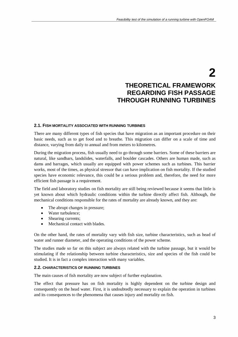
Impulse turbines use the water movement and the associated kinetic energy of a high-velocity jet
discharging at atmospheric pressure. (Turbak et al 1981).
Fig. 1 – Operating system of an Impulse Turbine (Source: [1])
With this system, shown in figure 1, suction on the down side of the turbine does not occur because
water flows through the bottom of the turbine after hitting the bucket. This type is usually used for
high head and low flow power schemes. The PELTON turbine is one example of impulse turbines and
the most used one.
Pelton turbines are one of the most important turbines when it comes to the conversion of hydraulic
energy into electricity, especially in mountain areas. As Dhakan P.K. and Chalil, A. B. P. (2013) refers
this is due to the fact that this type of turbines can be easily used in places where the altitude
difference between the water source and the location of the turbine is considerable.
Pelton turbines can be used in large scale hydro installation for heads that can go from 20 meters to
150 meters. Usually these types of turbines are not chosen when dealing with lower water heads since
the rotational speed becomes slower and the runner of the turbine required needs to be larger and it’s
difficult to manage.
In high water heads the flow rate tends to be lower going from 0,005 m3/s in the smaller systems till 1
𝑚3/s on larger systems. In consequence of these values the obtained power results can vary in a scale
from a few kW up to hundreds of MW’s in those larger systems.
Feasibility test of the simulation of a running turbine with OpenFOAM
5
In hydraulic systems with Pelton turbines, the reservoir is connected to a penstock head that is
posteriorly linked to a penstock where the water flows and is directed by a nozzle against the buckets
around the runner in a form of a thin jet.
These turbines can be arranged in two forms: in a horizontal shaft or in a vertical shaft. The horizontal
position allows the use of several runners leading to a higher specific speed and therefore a higher
operational speed. The vertical position allows a multi jet construction leading to an improvement of
the speed.
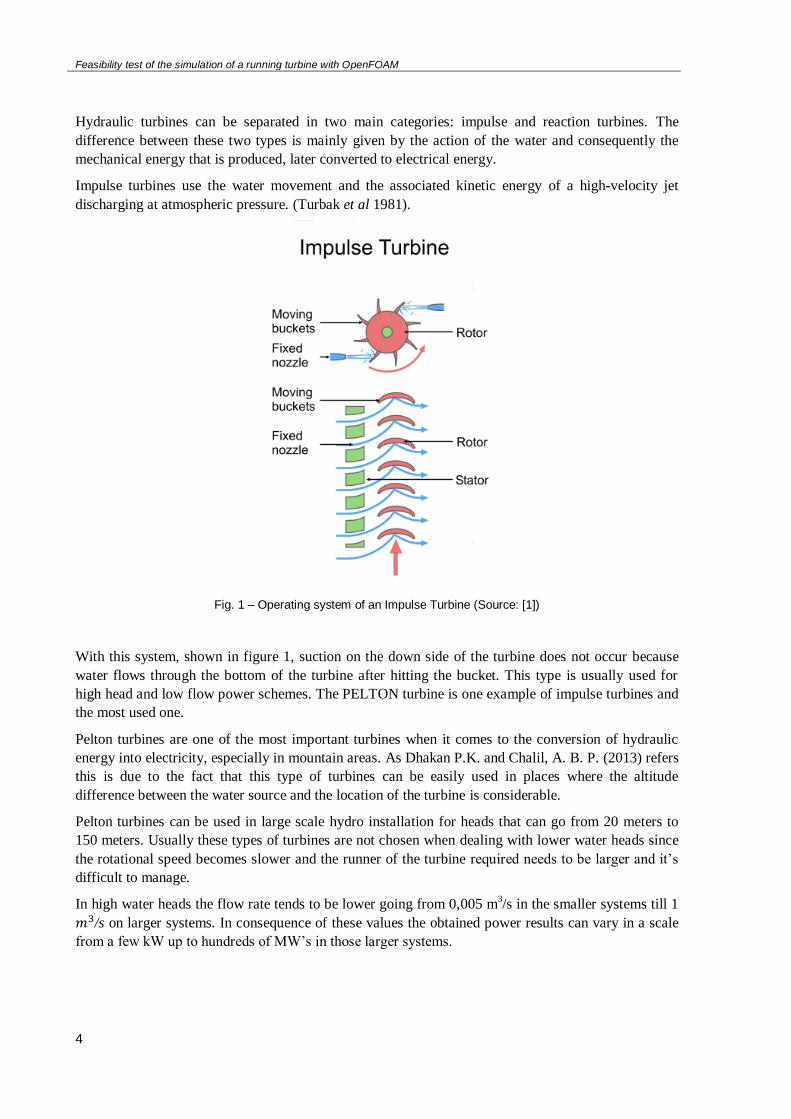
In reaction turbines, the flow system is restricted to a closed conduit and at any point it gets in contact
with air. This system is strictly closed from the headwater to the tail water. When water approaches
the runner it is provided with pressure energy and kinetic energy. The first is due to the density of the
water above this till the headwater surface and the second is due to the velocity. PROPELLER (Bulb
Turbine, Straflo, Kaplan) and FRANCIS are some of the examples of reaction turbines.
Fig. 2 – Operating system of a Reaction Turbine (Source [1])
As Turbak et al (1981) refers, fish mortality research has been almost entirely made with reaction
turbines and for this reason those type of turbines will be object of a more extensive explanation.
These turbines have a simple design that begins with an intake conduit that guides the water into the
main casing where it gets in contact with the nozzles that are attached to the rotor. The acceleration
caused by the water leaving the nozzles makes a reaction force on the pipes and consequently the rotor
starts moving in the opposite direction of the water.
The main shaft in the rotor can have different positions according to the different type of turbine. The
Straflo uses only horizontal flow but Francis and Kaplan can use both horizontal and vertical flow.
One of the most important and commonly used Propeller turbine is the Kaplan turbine. This turbine
has a propeller with adjustable blades inside a tube. It is also known as an axial-flow turbine meaning
that the flow direction doesn’t change while crossing the rotor.
Feasibility test of the simulation of a running turbine with OpenFOAM
6
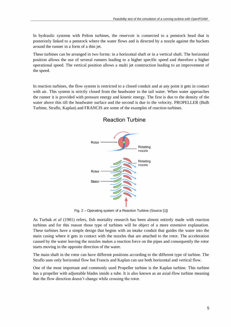
Theoretically, Kaplan turbines can work through an extensive spectrum of heads and flow rates, but, in
practice, there are other types of more effective turbines for higher heads of water. Due to this, Kaplan
turbines are usually chosen for lower water heads going from 1.5 to 20 meters with high flow rates
from 3 m3/s to 30 m
3/s. Hydroelectric power plants with Kaplan installations for these flows have
output power values from 75 kW to 1MW.
Fig. 3 – Basic layout of a Kaplan turbine (Source: [2])
These turbines have usually in their structure a nose cone, a rotor with adjustable blades and a vertical
driveshaft. The inlet guide-vanes that lead the water to the turbine can regulate the flow rate in the
turbine. This allows to fully stop the work of the turbine by closing completely the guide-vanes. It also
allows, depending on the position of the guide-vanes, to control the flow and consequently guarantee
that the oncoming flow can hit the rotor in the most efficient angle conducting to the highest
efficiency.
The blades can also be adjustable according to the dimension of the flow: a flat outline to very low
flows and a heavily-pitched outline for high flows. Allowing the adjustment of the inlet guide-vanes
leads to a big opening of the flow operating range and by adjusting the rotor blades it’s possible to
optimize the turbine efficiency.
Francis turbines are another type of really common reaction turbines and one of the most preferred
since they are also the most reliable turbines used in hydroelectric power stations.
Turbak et al (1981) states that the contribution of these turbines to the global hydropower capacity is
around 60 per cent, basically because the efficiency is higher under a huge range of different operating
conditions.
Installations with Francis turbines can operate in heads from 30 to 300 meters with flows from 10 to
700 m3/s and the number of blades in the turbine can vary from 14 in lower heads to 20 for higher
heads.
In a simplified way, the Francis turbine is composed of a runner with complex shaped blades. The
flow enters the turbine radially and leaves it axially as it is possible to notice on Fig. 4. Nevertheless
there is a particularity about the blades of the Francis turbine: the cross-section is shaped like a thin
airfoil. This means that when the inlet flow crosses the blades there is a low pressure in one side and a
high pressure on the other side, leading to a lift force.
Feasibility test of the simulation of a running turbine with OpenFOAM
7
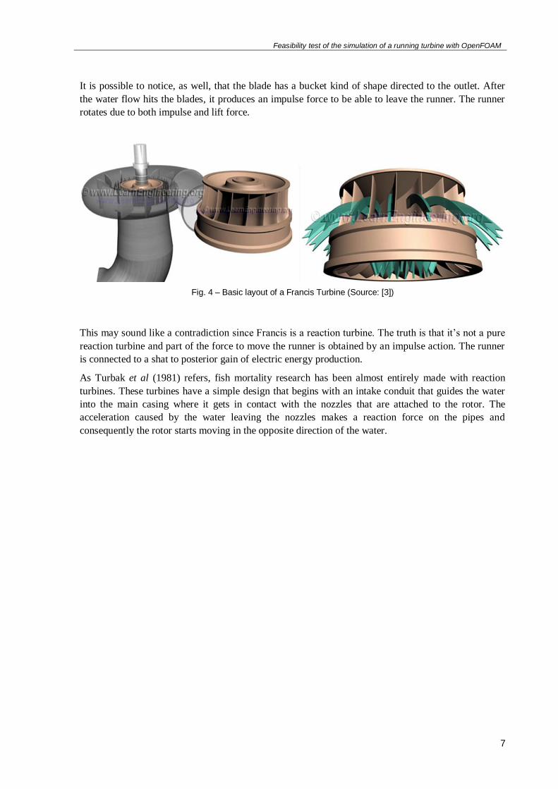
It is possible to notice, as well, that the blade has a bucket kind of shape directed to the outlet. After
the water flow hits the blades, it produces an impulse force to be able to leave the runner. The runner
rotates due to both impulse and lift force.
Fig. 4 – Basic layout of a Francis Turbine (Source: [3])
This may sound like a contradiction since Francis is a reaction turbine. The truth is that it’s not a pure
reaction turbine and part of the force to move the runner is obtained by an impulse action. The runner
is connected to a shat to posterior gain of electric energy production.
As Turbak et al (1981) refers, fish mortality research has been almost entirely made with reaction
turbines. These turbines have a simple design that begins with an intake conduit that guides the water
into the main casing where it gets in contact with the nozzles that are attached to the rotor. The
acceleration caused by the water leaving the nozzles makes a reaction force on the pipes and
consequently the rotor starts moving in the opposite direction of the water.
Feasibility test of the simulation of a running turbine with OpenFOAM
8
2.3. SOURCES OF FISH MORTALITY
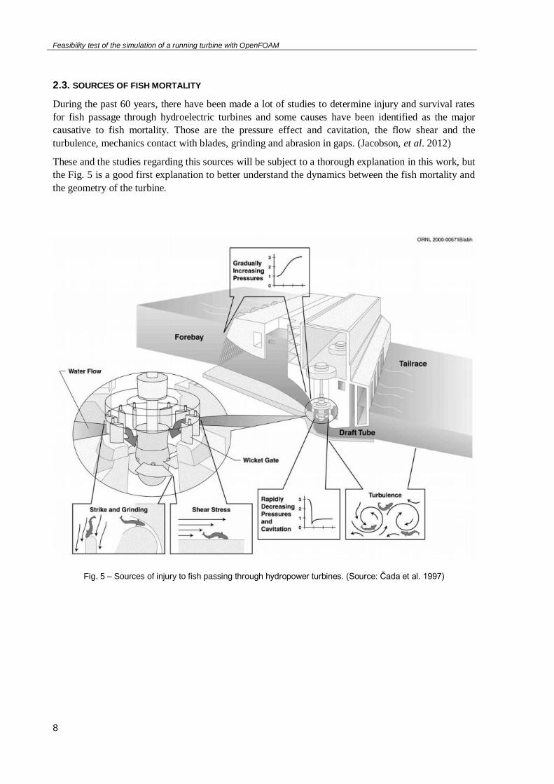
During the past 60 years, there have been made a lot of studies to determine injury and survival rates
for fish passage through hydroelectric turbines and some causes have been identified as the major
causative to fish mortality. Those are the pressure effect and cavitation, the flow shear and the
turbulence, mechanics contact with blades, grinding and abrasion in gaps. (Jacobson, et al. 2012)
These and the studies regarding this sources will be subject to a thorough explanation in this work, but
the Fig. 5 is a good first explanation to better understand the dynamics between the fish mortality and
the geometry of the turbine.
Fig. 5 – Sources of injury to fish passing through hydropower turbines. (Source: Čada et al. 1997)
Feasibility test of the simulation of a running turbine with OpenFOAM
9
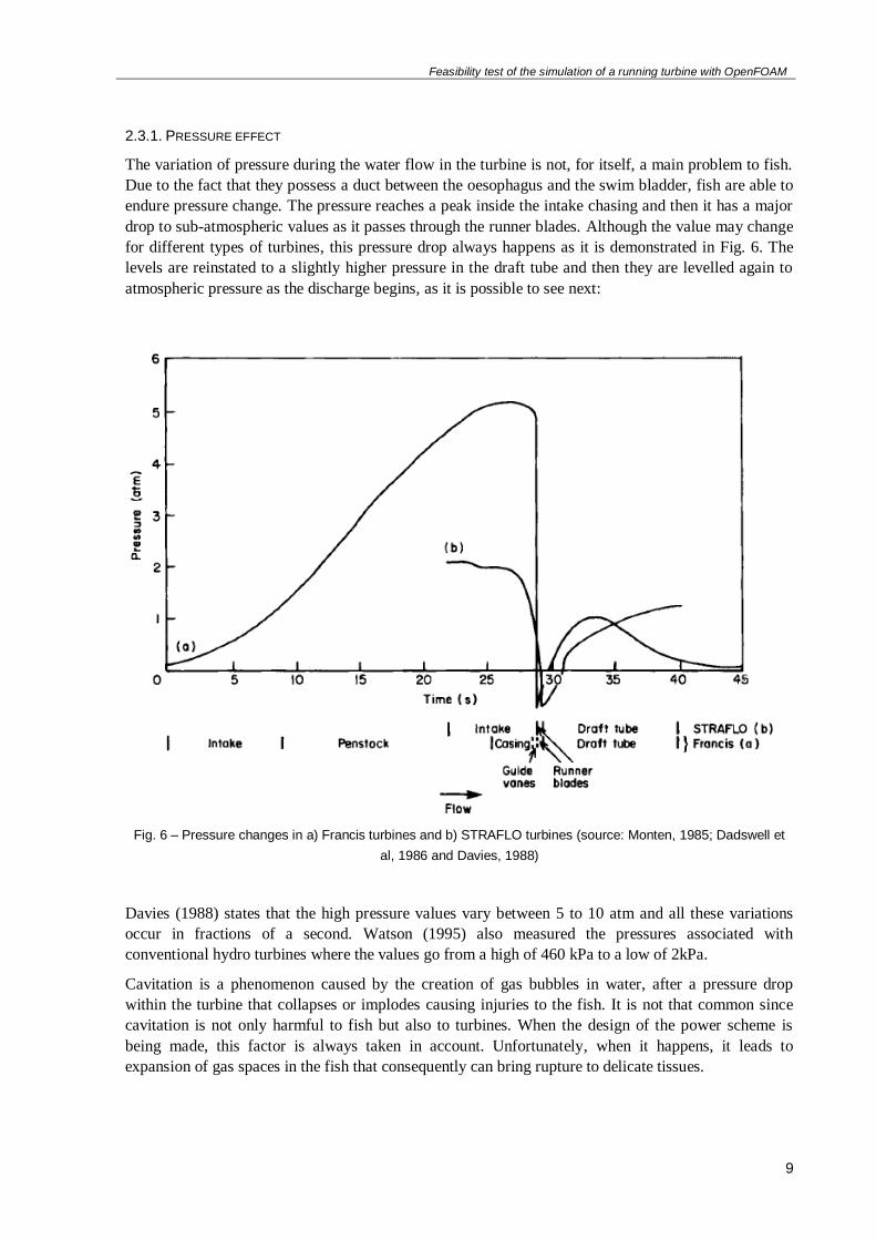
2.3.1. PRESSURE EFFECT
The variation of pressure during the water flow in the turbine is not, for itself, a main problem to fish.
Due to the fact that they possess a duct between the oesophagus and the swim bladder, fish are able to
endure pressure change. The pressure reaches a peak inside the intake chasing and then it has a major
drop to sub-atmospheric values as it passes through the runner blades. Although the value may change
for different types of turbines, this pressure drop always happens as it is demonstrated in Fig. 6. The
levels are reinstated to a slightly higher pressure in the draft tube and then they are levelled again to
atmospheric pressure as the discharge begins, as it is possible to see next:
Fig. 6 – Pressure changes in a) Francis turbines and b) STRAFLO turbines (source: Monten, 1985; Dadswell et
al, 1986 and Davies, 1988)
Davies (1988) states that the high pressure values vary between 5 to 10 atm and all these variations
occur in fractions of a second. Watson (1995) also measured the pressures associated with
conventional hydro turbines where the values go from a high of 460 kPa to a low of 2kPa.
Cavitation is a phenomenon caused by the creation of gas bubbles in water, after a pressure drop
within the turbine that collapses or implodes causing injuries to the fish. It is not that common since
cavitation is not only harmful to fish but also to turbines. When the design of the power scheme is
being made, this factor is always taken in account. Unfortunately, when it happens, it leads to
expansion of gas spaces in the fish that consequently can bring rupture to delicate tissues.
Feasibility test of the simulation of a running turbine with OpenFOAM
10
2.3.2. WATER TURBULENCE AND SHEARING CURRENTS
The turbulence that the water in a specific turbine can run is dependent on the Reynolds number
defined for it. The biggest problem concerning to fish is that this turbulence alters the water speed and
direction making the passage of fish in the turbine a difficult process. The main injuries registered are
contusions, abrasions, lacerations and sliced bodies leading in some cases to decapitation. Davies,
(1988).
Shearing currents are defined by two masses of water flow in different velocities and encountering
each other. This phenomenon is usual on the edges of the runner blades. Shear is easy to be identified
since it causes a specific damage to fish: the inversion of the gill arches and consequent decapitation.
Less common is the torn of the opercula and the damage of the gills. This can be easily understood,
because fish encounter themselves in a situation where different parts of their bodies are located in
masses of water with different velocities and directions.
2.3.3. MECHANICAL CONTACT WITH BLADES
The symptoms from this cause are most likely to be identified than the others. The injuries observed
by direct contact with the machinery are contusions, abrasions, lacerations or even complete
maceration. This is most likely to happen when the turbine is not working at its full capacity making
the path of the fish till the end more difficult. Many authors, such as Davies (1988) and Turbak et al
(1981), refer that the design of turbine as well as the fish length has a direct influence in the mortality
rate.
2.4. REVIEW ON STUDIES REGARDING THE SOURCES OF FISH MORTALITY
The studies made so far on fish mortality can be divided in two main categories: field observations and
laboratory simulation. In field, observation methods like netting, tagging, balsa boxes and floating tags
have been used to evaluate fish behaviour.
In laboratory, hydraulic conditions have been recreated in order to better expose what happens during
the passage of water through the turbine. In laboratory, it is more likely to control and observe how
pressure, runner diameter, head of water and other hydraulic conditions can affect fish physiologically
and anatomically.
There are a lot of the studies concentrated in the United States conducted with anadromous salmonids.
In the 1990’s, the studies were an important effort to protect the fish and to try to alert for the need of
downstream fish passage and protection facilities. (Jacobson, et al. 2012)
It is also important to mention that, in the 90’s, the Department of Energy developed the Advanced
Hydro Turbine Systems Program (AHTS) which main goal should be the improvement of turbine
technologies that could reduce the damage to entrained fish. Alongside with this, there were developed
two “fish-friendly” turbine designs so called as Alden turbine and Minimum Gap Runner Kaplan.
Nowadays, more recent studies have included also the blade strike experiments that are able to provide
data and guidelines for decreasing fish mortality by reshaping the leading edge of turbine blades.
(Jacobson, et al. 2012)
2.4.1. REVIEW OF PRESSURE STUDIES.
Laboratory evaluations were conducted by Harvey (1963), Foye and Scott (1965) after exposing fish,
more specifically Salmonids (physostomous) to gradual and rapid increase in pressure to 2,064 kPa
followed by decompression to atmospheric pressures. They concluded that this concrete action didn’t
show any significant mortality.
Feasibility test of the simulation of a running turbine with OpenFOAM
11
On the other hand, Harvey (1963) exposed the same specific species to pressures in the order of 84,6
kPa and the results regarding the mortality were significantly higher. Feathers and Knable (1983)
observed that using the pre-exposure to acclimation pressure as a variable made it possible to conclude
that fish mortality is related to the magnitude of depressurization.
Čada et al. (1997) also concludes that the highest mortalities were observed when the rate of pressure
decreases and the difference between the fish’s acclimation and the exposure pressure is higher.
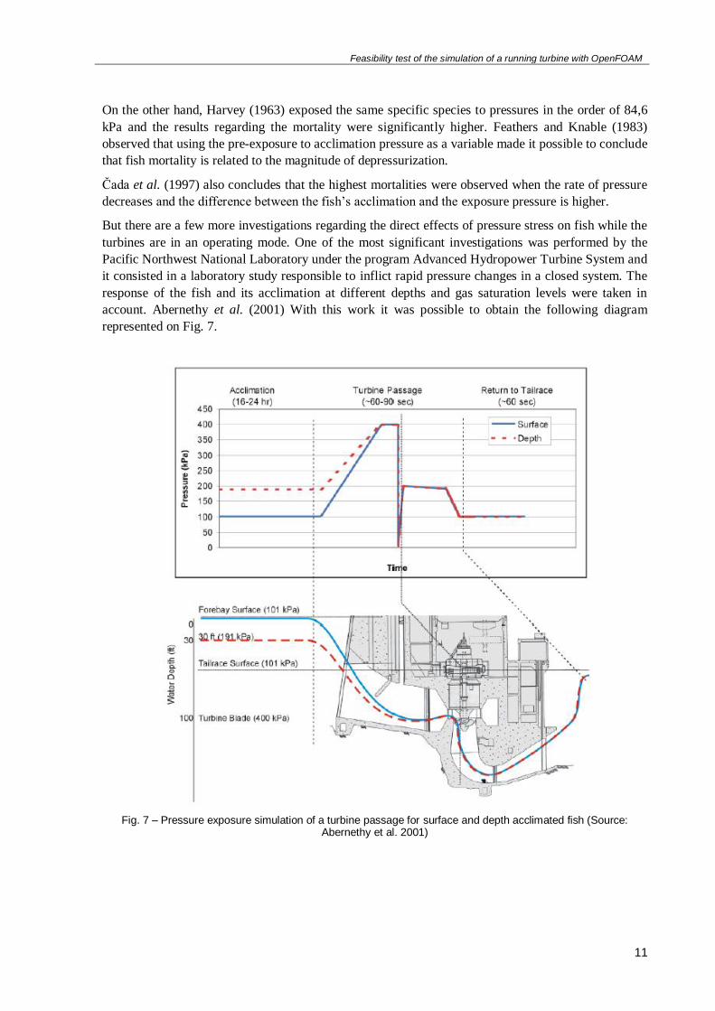
But there are a few more investigations regarding the direct effects of pressure stress on fish while the
turbines are in an operating mode. One of the most significant investigations was performed by the
Pacific Northwest National Laboratory under the program Advanced Hydropower Turbine System and
it consisted in a laboratory study responsible to inflict rapid pressure changes in a closed system. The
response of the fish and its acclimation at different depths and gas saturation levels were taken in
account. Abernethy et al. (2001) With this work it was possible to obtain the following diagram
represented on Fig. 7.
Fig. 7 – Pressure exposure simulation of a turbine passage for surface and depth acclimated fish (Source: Abernethy et al. 2001)
Feasibility test of the simulation of a running turbine with OpenFOAM
12
Resorting to CFD modeling allows the investigators to better control the chosen pressure regimes
while having the possibility to change the operating conditions. It is also possible to achieve a model
of pressure-induced mortality by the collection of empirical data.
One of the first successful works in this field was accomplished by Tumpenny et al. (2000) by
resorting to CFD simulation to reach a method were it was possible to predict the injury rates resultant
from damaging pressures for low-head Francis and Kaplan turbines. It was also concluded that the
turbine runner and the draft tube of the turbines are the main risk areas of injuries related to pressure.
One of the most recent study made by Brown et al. (2007) supported all these conclusions by
demonstrating that acclimation pressure is a significant predictor for the risk of injury or death but
only when fish are exposed to lower pressures in the order of 8 to 19kPa.
2.4.2. REVIEW OF WATER TURBULENCE AND SHEARING CURRENTS STUDIES.
Turbulence is defined as the fluctuations in velocity magnitude and direction associated with the
movement of the water and, precisely by this, studies in this field are more difficult to evaluate than all
the others. Since in turbulent flows there are also shear forces, this creates an obstacle to clearly
understand the different effects these two elements have on fish.
The physical effects of shear and turbulence on a fish organism are most likely the same. However, it
is likely that turbulence does not have a direct effect on fish mortality but can contribute with
disorientation, especially when fish are leaving the draft tube. (Čada et al. 1997)
Killgore et al. (1987) studied the survival of fish (more precisely paddlefish yolk-sac larvae) when
exposed to different frequencies and intensities of turbulence created by barges. He got to the
conclusion that low turbulence levels, in the order of 22-23 cm/s, would lead to low rates of mortality
around 13%. On the other hand, high turbulence levels, such as 57-59 cm/s, could engage in mortality
levels around or higher than 80%.
The main studies regarding shear currents have two main difficulties: correlating injury and mortality
with shear levels experienced by individual fish that are collected after turbine passage and distinguish
these injuries from similar injuries that can have other causes, like blade strikes for example.
(Jacobson, 2012)
It is natural to assume that velocities and magnitudes of shear stress along the path that fish have to
make through turbines is much higher than in their natural environments. Velocity inside a turbine was
measured varying from zero near solid boundaries to approximately 36,58 m/s (120 ft/s) in areas away
from the boundaries. Resorting to these values, the estimations of shear stress values for bulb turbine
draft tubes would go from 500 to 5,400 N/m2 with stress levels under 1,000 N//m2 in over 90% of the
passage zone. (McEwen and Scobie 1992).
Based on the previous study, Turnpenny et al. (1992) began a laboratory experience where fish were
exposed to a high-velocity water jet in a static water tank. After exposing the fish to the shear stress
that was created it was possible to get to the conclusion that values of shear stress bellow 774 N//m2
are not harmful neither can lead to death. Other important result of this study was that mortality was
proportional to jet velocity as well as the fish orientation at the initial exposure.
To have better conclusions regarding this subject, computer modelling techniques were applied in
order to better characterize the variation of shear forces throughout the entire turbine, especially on the
surroundings of the runner blades and other structural components. Turnpenny et al. (2000) applied
Computational Fluid Dynamic (CFD) modelling to low-head Francis and Kaplan turbines in order to
Feasibility test of the simulation of a running turbine with OpenFOAM
13
better identify the possibility of injury due to shear stress. The conclusion was that the shear stress
levels were of minor importance since they had low probabilities of occurring. Investigators predicted
that less than 2% of the fish passing low-head turbines would suffer fatal injuries due to shear stress.
2.4.3. REVIEW OF MECHANICAL STUDIES.
The possibility to engage in direct observation within turbines is in fact difficult and by that fact it was
calculated the strike probability and defined that almost every strike, if not all, could cause mortality.
This early models were developed to estimate the blade strike probability taking into account factors
like flow velocity, blade and guide vane angles, blade rotational speed and the length of the fish. (Von
Raben 1957 and Solomon 1988).
Turnpenny et al. (1992) conducted an experience doing the simulation of the strike speeds near the
hub and the blade tip. These experiments had taken into account the different blade profiles and how
they could lead to different results if conjugated with different fish sizes, orientation and position
relative to the blade. The conclusions were that regardless the outline of the blades, the results would
vary only with the change of the blades velocity. For high velocities severe damages were registered,
like bruising, internal bleeding and broken spines and on the other hand, with low velocities, little
damage and no mortality were observed. In the same study, it was possible to build a pattern regarding
the orientation of a fish relative to the blade. The conclusion was that for fish weighing under 20g the
harm was minor, since they were swept aside by the blade. On the other hand, for fish weighing up to
200g the chance of being hit when their centre of gravity was coincident with the blade’s path was of
75%. (Turnpenny et al. 1992)
As a follow up for these studies, Turnepenny et al. (1992) established equations for low-head, axial-
flow tidal turbines taking into account blade strike probabilities, fish length, fish location, fish
orientation, fish swimming speed, flow velocity, open space between blades, blade leading edge
thickness and blade speed.
Later, Turnpenny et al. (2000) adapted the statistical methods to predict injury rates for smaller
turbines. Results correlated the fish size, turbine type, runner diameter and rotational rate (rpm),
number of blades and operating load to the strike injury. Another conclusion was that by altering the
design of the turbine, like the number and length of blades or the area per blade channel, the
probability of the strike could be diminished.
A pilot-scale laboratory study with multiple fish species and sizes and with two operating heads –
12,19 m (40ft) and 24,38 m (80ft) - different operating efficiencies and without wicket gates was
conducted in order to evaluate the relation between the operating conditions and its respective fish
mortality. One of the main conclusions was that the depth, the turbine efficiency and the presence or
not of wicked gates had no statistic influence on fish mortality or injury rates. (Hecker et al. 2002;
Amaral et al. 2003; Cook et al. 2003).
As it is predictable, independently of the turbine design, fish mortality increases with fish size
augmentation. To support this conclusion, pilot-scale test data and a strike probability model of a
standard turbine blade were used to estimate the strike probability in a full-scale prototype unit for the
heads already evaluated – 12,19m and 24,38m. It was conclude that there are high survival rates,
higher than 96% for fish, with a length equal or less than 200mm for both operating heads.

Feasibility test of the simulation of a running turbine with OpenFOAM
14
Feasibility test of the simulation of a running turbine with OpenFOAM
15
3 Computational Fluid Dynamics –
CFD
3.1. INTRODUCTION TO COMPUTATIONAL FLUID DYNAMICS
Computational Fluid Dynamics is the field in fluid mechanics that studies the resolution and analysis
of the flow using algorithms and numerical methods.
Fluids numerical modelling started, almost exclusively, with aeronautical study, but nowadays it is
used in several areas of engineering and physics. It is employed in areas such as aircraft, turbo
machinery, car and ship design and it can also be applied in areas such as meteorology, oceanography,
astrophysics, oil recovery and also architecture. In its beginnings, it was a combination of physics,
numerical mathematics and some computer science simulating fluid flows. With the advance in
computer technology, it also occurred an advance in computational fluid dynamics. From simulating
transonic flows based on the solution of non-linear potential equations, the CFD applications evolved
to the first two-dimensional solutions and afterwards to three dimensional solutions. (Blazek. 2001)
With the promptly increasing computers capacity and speed, it was possible to start developing some
more robust simulations with inviscid flows passing complete aircrafts configurations or inside turbo
machines. With this development, it came the need to start more demanding simulation with viscous
flows governed by the Navier Stokes equations. As a result, turbulence models such as Reynolds-
average Simulation (RAS) and the Large Eddy Simulation (LES) appeared. (Blazek. 2001)
With the consequent advance of the complexity in flow simulations, the grid generation also had to
follow this development. The progress started first with simple structured meshes constructed either by
algebraic methods or by using partial differential equations. But with increasing geometrical
complexity of the configurations, the grids had to be broken into a number of topologically simpler
blocks and then the multiblocks approach appeared. Nevertheless, the generation of a complex
structure using multiblocks grid would still take a long time in the order of weeks or even months. Due
to this fact, the research on the field of unstructured grid generators and consequently its solver took a
big growth by promising to reduce the setup times. (Blazek. 2001)
With the use of the Navier-Stokes equations, the requirements for the meshes were more demanding.
Prisms and hexahedra grids in viscous flows began to be used, improving the solution accuracy and
saving the number of elements, faces and edges.
The biggest problem on using fluids numerical modelling software is the greatest complexity and
unpredictability on knowing how a fluid will behave since it has a non-linear behaviour. Despite this
problem, with the appearance of more powerful computers, the properties of the fluids are more easily
understood. Another problem is that the obtained solutions are only as correct as the physical models
they are based on.
Feasibility test of the simulation of a running turbine with OpenFOAM
16
The simulation with physical models involving fluids is very expensive. A physical model, depending
on its complexity, needs a large set of material to better represent the prototype but it also needs
measurement material and specialized staff. In spite of all these disadvantages, Bakker (2002) refers
some important advantages, such as the cost reduction, since the computers became more advanced
and faster in order to obtain results. One of the biggest advantages is the ability to simulate real
conditions, such as flow and heat transfers and also to be able to control the physical process,
isolating, if necessary, one specific phenomena.
With the advance of technology, it is already possible to run some of these experiments on personal
computers. Also with the growing of CFD simulations, there is already in the market some software
that can be used without any cost to the user, such as OpenFOAM.
Despite all the advantages Versteeg and Malalasekera (1995) refer that the numerical errors and the
boundary conditions are two of the biggest problems when programming in CFD. Factors like the
ambient temperature or the existence of air bubbles are not always included on the modelling process
and that leads to calculation errors.
Numerical errors are the most frequent and they usually occur because of the algorithms used in CFD
software which use really complex mathematical equations. Such as the experiments and simulations
in physical models, the CFD simulations need a critical review of the results in order to be validated.
3.2. SPECIAL FEATURES OF THE CFD TOOLS
The base knowledge behind numerical modelling of fluids is that the numerical algorithms are able to
simulate the fluid behaviour. Versteeg and Malalasekera (1995) refer three main elements: a pre-
processor, a solver and a post-processor.
3.2.1 PRE-PROCESSOR
This stage is where all the physical properties and information about the flow are defined. The data
that is necessary is:
definition of the region in study;
definition of the geometry of the study case through meshes;
definition of both physical and chemical properties of the model in study;
definition of the fluid properties;
definition of boundary conditions.
The definition of the mesh in a CFD problem is the first step to get the answer for a flow problem. The
velocity, pressure and temperature, among other characteristics, are defined at the various nodes inside
every cell of the mesh. As it is easy to understand, the precision of the result is largely dependent on
the number of cells of the mesh. The larger the number of cells, the biggest is the accuracy of the
solution. Efficient meshes should not be uniform: thinner in areas where big variations of
characteristics happen and larger where this doesn’t happen. The evolution on CFD is to try to make
the programs with the ability to create these different meshes by themselves but for now it is still up to
the user to make the better judgement about the correct mesh to use.

Feasibility test of the simulation of a running turbine with OpenFOAM
17
3.2.2. SOLVER
It’s possible to obtain solutions by three different types of resolution: finite difference, finite element
and spectral methods. As Versteeg and Malalasekera (1995) refer, the three are governed by the same
assumptions: the ability to approximate the unknown flow variables with simple functions, to
transform a continuous distribution in discrete units and then to approximate these into the governing
flow equations and their respective mathematical manipulations.
The finite difference method has the approximation to the Navier-Stokes equations in their simplified
form and it’s of easy implementation. On the other side, it generates problems along the curved
boundaries, such as the difficulty in achieving stability and reaching a convergence in the analysis.
The mesh adaptation is also difficult.
The finite volume method is an approximation of the Navier-Stokes equations as a system of
conservation equations being the biggest advantage the fact that the special discretisation is carried out
directly in the physical space. The disadvantages are that, like the previous one, it has difficult stability
and convergence analysis and it’s difficult to adapt to unstructured meshes.
The spectral method evaluates the spatial derivatives resorting to Fourier series or one of their
generalizations. It is possible to obtain the biggest advantage from spectral methods if the functions
used are periodic and the grid points uniformly spaced. Any change in geometry or boundary
conditions requires a considerable change in the method, making these methods relatively inflexible.
As it’s possible to conclude, the biggest difference between these three streams is the way the flow
variables are approximated and consequently the discretisation process. These methods will be further
explored in chapter 3.7. (Ferziger, J.H. 2002)
3.2.3. POST-PROCESSOR
A big development has been done in the post-processing field. Almost all of CFD software is equipped
with different visualization tools that can be divided into two forms: graphically or alphanumerically.
In the graphical tools, there are vector plots, geometry and grid display contours, iso-surfaces,
flowlines and animations. In the alphanumeric tools, there are some such as integral values, drag, lift
and torque calculations, averages and standard deviations. These tools can facilitate the perception that
the user has about work in progress.
Fig. 8 – Flow around a cylinder: grid. (Source: Baker, 2002)
Feasibility test of the simulation of a running turbine with OpenFOAM
18
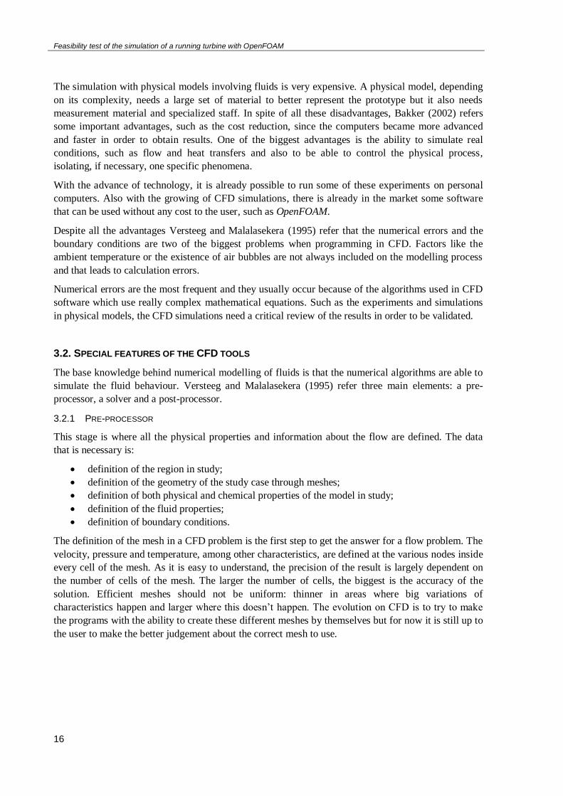
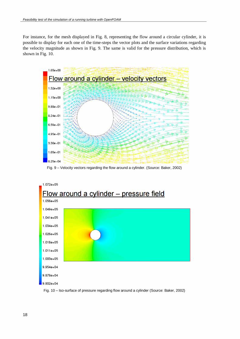
For instance, for the mesh displayed in Fig. 8, representing the flow around a circular cylinder, it is
possible to display for each one of the time-steps the vector plots and the surface variations regarding
the velocity magnitude as shown in Fig. 9. The same is valid for the pressure distribution, which is
shown in Fig. 10.
Fig. 9 – Velocity vectors regarding the flow around a cylinder. (Source: Baker, 2002)
Fig. 10 – Iso-surface of pressure regarding flow around a cylinder (Source: Baker, 2002)

Feasibility test of the simulation of a running turbine with OpenFOAM
19
As it’s possible to acknowledge, the post-processor is as important as the rest of the procedure
allowing the user to rightly obtain conclusions.
3.3. MESHES
Analytical solutions are not usually a possible answer for the differential equations used to solve fluid
flow and heat transfer problems due to the complexity and non-linearity of the governing equations. In
order to better analyse the fluid flows, the domains are divided into smaller subdomains. These
subdomains are characterized by geometric shapes like hexahedra and tetrahedral in 3 dimensions and
quadrilaterals and triangles in 2 dimensions.
The biggest help on doing this type of division is that the equations are now solved inside each one of
these smaller domains. The methods used to solve this equation were previously mentioned in the
chapter 3.2.2 - Solver. These subdomains or cells must have a logical continuity so the solution
obtained across the different points can make sense when put all together. All these elements are
called a mesh or a grid.
Meshes can be rearranged in different forms and they can be structured or unstructured. Structured
meshes (see Fig. 11) follow a i,j,k convention as opposite to unstructured meshes that don’t have any
convention (see Fig. 12). It is also possible to have multiblocks that consist in a group of meshes each
of which can be structured or unstructured.
Fig. 11 – Structured mesh (Source: Yoganathan et al. 2004)
Fig. 12 – Unstructured mesh (Source: Yoganathan et al. 2004)
Feasibility test of the simulation of a running turbine with OpenFOAM
20
As it’s possible to notice, the biggest difference on the two types of meshes is that the first one has the
topology of a square grid of parallelepipeds, but the same does not happen on the second. These two
types of meshes can be unpredictably difficult to generate, especially because a mesh that can be used
to evaluate fluid flows, for instance, needs to satisfy some limits that are hard to achieve. A mesh must
represented as accurate as possible the object in study, but always with the restriction on size and
shape of the elements of the mesh.
Modelling objects with complex shapes, as is the case of a turbine, obligates many times the use of
curved surfaces. And with these surfaces two types of boundaries appear: exterior and interior
boundaries.
As Shewchuk (1997) refers, exterior boundaries separate meshed and unmeshed portions of space, and
are found on the outer surface and in the internal holes of a mesh. On a different point of view, internal
boundaries appear within meshed portions of space, and enforce the constraint that elements may not
pierce them. These boundaries are typically used to separate regions that have different physical
properties. The size of the elements is an important control that should be also done while generating
the mesh. This means that the variation of size of the elements should be done in a short distance. And
why should this happen? The size of the elements has an influence on the finite element simulation.
The smaller the elements are and more densely packed, the biggest is the accuracy of the results, but at
the same time this is going to increase the required time for the computer to solve the problem. Of
course that the physical phenomena in study has a highly influence on the size chosen for the
elements. For instance, in a fluid flow simulation, in areas where turbulence occurs, the elements
should be smaller than in areas of steadiness.
It is possible to have the same size of elements through all the domain in study but that can lead to
excessive computational demands. One way to solve this problem is to use a mesh generator that can
make the gradation from small to large sizes of the elements inside the mesh. Mesh generator
algorithms have the main goal to generate a mesh with as few elements as possible offering the option
to refine some parts of the mesh where the elements are not as small as required.
In conclusion, the last aim of generating a mesh is to try to make the elements as “round” as possible
in shape because angles (as big or small they can be) degrade the quality of the solution.
The quality of each element is still a relative subject, highly dependent on the model in study, the type
of numerical method used and the polynomial degree of the piecewise functions used to interpolate the
solution over the mesh.
Feasibility test of the simulation of a running turbine with OpenFOAM
21
3.4. MAIN PRINCIPLES ABOUT FLUID DYNAMICS
Before proceeding to the study of fluid dynamics, it is important to have some ground notions of how
fluids work. Fluids are substances whose molecular structure is not affected by external shear forces.
Common dynamic forces like pressure differences, gravity, shear, rotation and surface tension are the
responsible for the fluid flow.
The software that runs numerical modelling of fluids has its base ground on some fundamental
conservation laws of fluids. Those are:
Mass conservation (Continuity law)
The rate of change of momentum equals the sum of the forces on a fluid particle (Second law
of Newton)
Conservation of energy in a particle (First law of thermodynamics)
The numerical formulation of these principles can be written in a differential way. When the study is
done in an integral way, it’s necessary to consider the change of mass, movement or energy inside the
volume where the inflow and the outflow of the fluid occur. In a differential study, it is used the
Stokes equation where the conservative laws are applied to an infinitesimal volume. It’s in this last
assumption that the majority of the fluid dynamics modelling is based on.
The velocity of a flow is also an important characteristic and allied with the inertia of the fluid it
defines if the flow is laminar or turbulent. As the velocity increases and it leads to instability and to a
more random type of flow the flows goes from laminar to turbulent.
3.4.1. MASS CONSERVATION – LAW OF CONTINUITY
The continuity law states that, in the mass conservation, the rate of increase of mass in the fluid
element needs to be equal to the net rate of flow of mass into the same fluid element.
This can be described by the following equation:
Where ρ defines the fluid density, u⃗ , the absolute velocity of the fluid and n⃗ , the unit vector normal
to the element with the area dA. The indices cv and cs have the meaning of control volume and control
surface, referring to the fluid element.
Defining a fluid element with sides such as δx, δy and δz , as its shown in the Fig. 13, can make the
understanding of mass conservation easier.
𝜕
𝜕𝑡∫ 𝜌𝑑 𝑉
𝑐𝑣
+ ∫ 𝜌�⃗�
𝑐𝑠
× �⃗� 𝑑𝐴 = 0 (3.1)
Feasibility test of the simulation of a running turbine with OpenFOAM
22
Fig. 13 – Fluid element for conservation laws (Source: Baker, 2002)
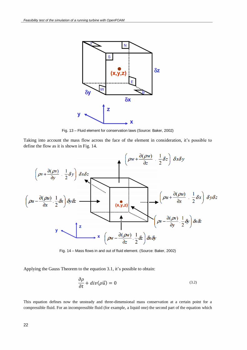
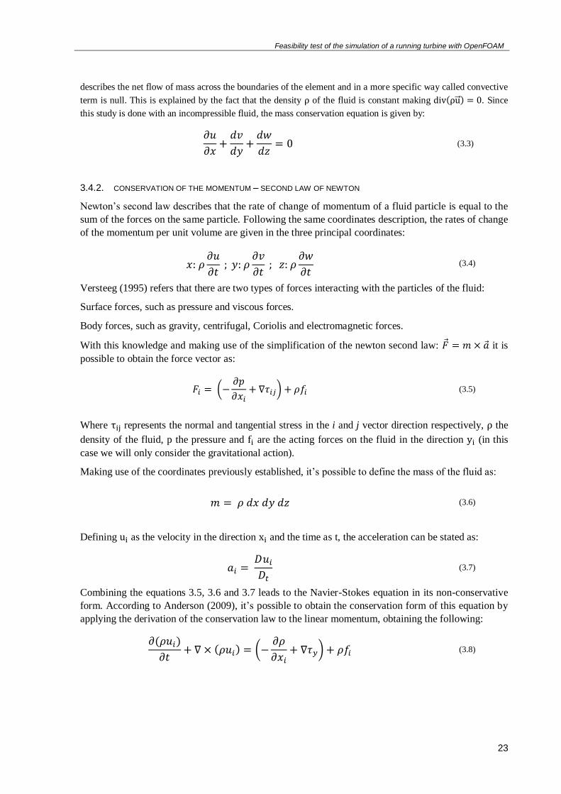
Taking into account the mass flow across the face of the element in consideration, it’s possible to
define the flow as it is shown in Fig. 14.
Fig. 14 – Mass flows in and out of fluid element. (Source: Baker, 2002)
Applying the Gauss Theorem to the equation 3.1, it’s possible to obtain:
This equation defines now the unsteady and three-dimensional mass conservation at a certain point for a
compressible fluid. For an incompressible fluid (for example, a liquid one) the second part of the equation which
𝜕𝜌
𝜕𝑡+ 𝑑𝑖𝑣(𝜌�⃗� ) = 0 (3.2)
Feasibility test of the simulation of a running turbine with OpenFOAM
23
describes the net flow of mass across the boundaries of the element and in a more specific way called convective
term is null. This is explained by the fact that the density ρ of the fluid is constant making div(ρu⃗ ) = 0. Since
this study is done with an incompressible fluid, the mass conservation equation is given by:
3.4.2. CONSERVATION OF THE MOMENTUM – SECOND LAW OF NEWTON
Newton’s second law describes that the rate of change of momentum of a fluid particle is equal to the
sum of the forces on the same particle. Following the same coordinates description, the rates of change
of the momentum per unit volume are given in the three principal coordinates:
Versteeg (1995) refers that there are two types of forces interacting with the particles of the fluid:
Surface forces, such as pressure and viscous forces.
Body forces, such as gravity, centrifugal, Coriolis and electromagnetic forces.
With this knowledge and making use of the simplification of the newton second law: 𝐹 = 𝑚 × 𝑎 it is
possible to obtain the force vector as:
Where τij represents the normal and tangential stress in the i and j vector direction respectively, ρ the
density of the fluid, p the pressure and fi are the acting forces on the fluid in the direction yi (in this
case we will only consider the gravitational action).
Making use of the coordinates previously established, it’s possible to define the mass of the fluid as:
Defining ui as the velocity in the direction xi and the time as t, the acceleration can be stated as:
Combining the equations 3.5, 3.6 and 3.7 leads to the Navier-Stokes equation in its non-conservative
form. According to Anderson (2009), it’s possible to obtain the conservation form of this equation by
applying the derivation of the conservation law to the linear momentum, obtaining the following:
𝜕𝑢
𝜕𝑥+
𝑑𝑣
𝑑𝑦+
𝑑𝑤
𝑑𝑧= 0 (3.3)
𝑥: 𝜌𝜕𝑢
𝜕𝑡 ; 𝑦: 𝜌
𝜕𝑣
𝜕𝑡 ; 𝑧: 𝜌
𝜕𝑤
𝜕𝑡 (3.4)
𝐹𝑖 = (−𝜕𝑝
𝜕𝑥𝑖+ ∇𝜏𝑖𝑗) + 𝜌𝑓𝑖 (3.5)
𝑚 = 𝜌 𝑑𝑥 𝑑𝑦 𝑑𝑧 (3.6)
𝑎𝑖 = 𝐷𝑢𝑖
𝐷𝑡 (3.7)
𝜕(𝜌𝑢𝑖)
𝜕𝑡+ ∇ × (𝜌𝑢𝑖) = (−
𝜕𝜌
𝜕𝑥𝑖+ ∇𝜏𝑦) + 𝜌𝑓𝑖 (3.8)
Feasibility test of the simulation of a running turbine with OpenFOAM
24
The fluids in study – water and air – are so called Newtonian fluids. This means that the shear stress in
these fluids is proportional to the velocity gradients. Using 𝜇 as the correspondence to the viscosity of
the fluid, it is possible to simplify the conservative formula into the following:
3.4.3. CONSERVATION OF ENERGY IN A PARTICLE - FIRST LAW OF THERMODYNAMICS
The energy equation is possible to be obtained through the first law of thermodynamics that says that
the rate of increase of the energy of a fluid particle is the sum of the net rate of heat added to the fluid
particle with the net rate of work done on the same fluid particle.
It is possible to obtain the rate of heat addition to the fluid particle due to heat conduction across the
element boundaries through the next equation referred by Versteeg (1995):
Where q represents the heat flux, k, the thermal conductivity and T, the temperature.
Still according to this author, the net rate of energy added by work forces acting on the fluid can be
described as:
Where 𝜌𝑓 × �⃗� represents the gravity force acting on the fluid and the rest of the equations represents
the work transfer caused by the forces acting on the surface in study.
It is also know that the total energy on a fluid per mass unit is given by the sum of the internal energy,
𝑒, with the kinetic energy, 𝑢2
2. The total energy is given by:
Connecting all the previous equations regarding energy, it is possible to get to the final equation in a
non-conservative way:
𝜌 [𝜕𝑢𝑖
𝜕𝑡+
𝜕(𝑢𝑖 + 𝑢𝑗)
𝜕𝑥𝑖
] = −𝜕𝑝
𝜕𝑥𝑖+ 𝜇
𝜕2𝜇𝑖
𝜕𝑥𝑗2 + 𝜌𝑓𝑖 (3.9)
−∇𝑞 = ∇(𝑘∇ 𝑇) (3.10)
∇(𝑝�⃗� ) + [∑∇(𝑢𝑗 × 𝜏𝑖𝑗)] + 𝜌𝑓 × �⃗� (3.11)
𝜌𝐷
𝐷𝑡(𝑒 +
𝑢2
2) (3.12)
𝜌𝐷
𝐷𝑡(𝑒 +
𝑢2
2) = ∇(𝑘∇ 𝑇) + ∇(𝑝�⃗� ) + [∑∇(𝑢𝑗 × 𝜏𝑖𝑗)] + 𝜌𝑓 × �⃗� (3.13)
Feasibility test of the simulation of a running turbine with OpenFOAM
25
3.5. TURBULENT FLOW
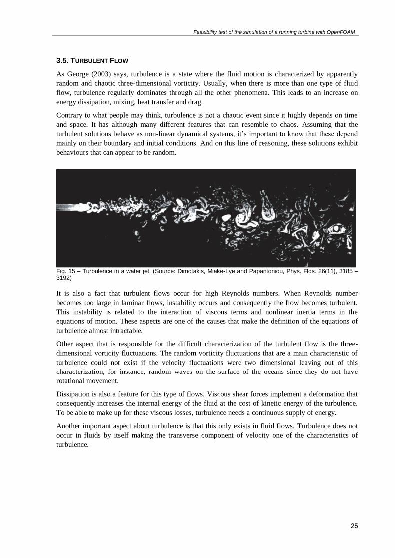
As George (2003) says, turbulence is a state where the fluid motion is characterized by apparently
random and chaotic three-dimensional vorticity. Usually, when there is more than one type of fluid
flow, turbulence regularly dominates through all the other phenomena. This leads to an increase on
energy dissipation, mixing, heat transfer and drag.
Contrary to what people may think, turbulence is not a chaotic event since it highly depends on time
and space. It has although many different features that can resemble to chaos. Assuming that the
turbulent solutions behave as non-linear dynamical systems, it’s important to know that these depend
mainly on their boundary and initial conditions. And on this line of reasoning, these solutions exhibit
behaviours that can appear to be random.
Fig. 15 – Turbulence in a water jet. (Source: Dimotakis, Miake-Lye and Papantoniou, Phys. Flds. 26(11), 3185 – 3192)
It is also a fact that turbulent flows occur for high Reynolds numbers. When Reynolds number
becomes too large in laminar flows, instability occurs and consequently the flow becomes turbulent.
This instability is related to the interaction of viscous terms and nonlinear inertia terms in the
equations of motion. These aspects are one of the causes that make the definition of the equations of
turbulence almost intractable.
Other aspect that is responsible for the difficult characterization of the turbulent flow is the three-
dimensional vorticity fluctuations. The random vorticity fluctuations that are a main characteristic of
turbulence could not exist if the velocity fluctuations were two dimensional leaving out of this
characterization, for instance, random waves on the surface of the oceans since they do not have
rotational movement.
Dissipation is also a feature for this type of flows. Viscous shear forces implement a deformation that
consequently increases the internal energy of the fluid at the cost of kinetic energy of the turbulence.
To be able to make up for these viscous losses, turbulence needs a continuous supply of energy.
Another important aspect about turbulence is that this only exists in fluid flows. Turbulence does not
occur in fluids by itself making the transverse component of velocity one of the characteristics of
turbulence.
Feasibility test of the simulation of a running turbine with OpenFOAM
26
3.6 TURBULENCE MODELS
As it was said before, turbulence causes the appearance of a big variety of vortices that make the
resolution of this type of cases even more difficult.
Versteeg (1995) states that the computational fluid dynamic models, that solve a turbulence problem,
should be accurate, simple, economical to run and with a wide applicability. Subsequently, they define
three different models:
Reynolds Averaged Navier-Stokes (RANS)
Large Eddy Simulation (LES)
Direct Numerical Simulation (DNS)
3.6.1. MODELS BASED ON REYNOLDS AVERAGED NAVIER-STOKES
Turbulent flows are characterized by the variation of velocity during time and space. These flow
problems can be solved using the Navier-Stokes equations although it leads to a very long and difficult
process. To simplify this process, the Reynolds equations are commonly used, leading to the group
already mentioned as Reynolds averaged Navier-Stokes.
Engineers usually focus their attention on certain mean quantities which are velocities, pressures or
stresses. Nevertheless, when it comes to execute the time-averaging operation on the momentum
equations, the state of the flow contained in the instantaneous fluctuations is neglected and it is
sufficient to consider the time mean of the flow properties.
For this reason, the Reynolds Averaged Navier-Stokes is one of the most popular models.
This model introduces in the time averaged momentum equations six supplementary unknowns
defined as Reynolds stresses.
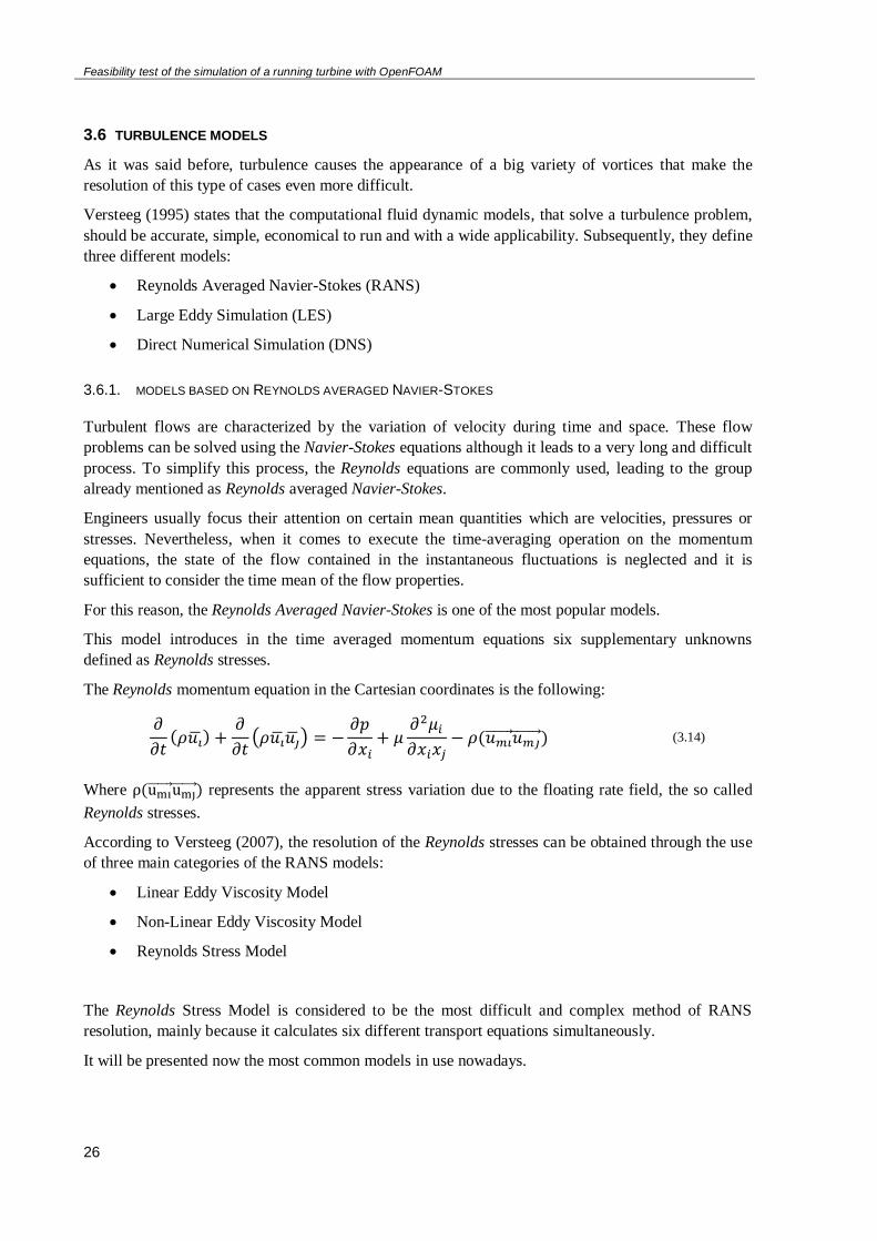
The Reynolds momentum equation in the Cartesian coordinates is the following:
Where ρ(umi⃗⃗ ⃗⃗ ⃗⃗ umj⃗⃗ ⃗⃗ ⃗⃗ ) represents the apparent stress variation due to the floating rate field, the so called
Reynolds stresses.
According to Versteeg (2007), the resolution of the Reynolds stresses can be obtained through the use
of three main categories of the RANS models:
Linear Eddy Viscosity Model
Non-Linear Eddy Viscosity Model
Reynolds Stress Model
The Reynolds Stress Model is considered to be the most difficult and complex method of RANS
resolution, mainly because it calculates six different transport equations simultaneously.
It will be presented now the most common models in use nowadays.
𝜕
𝜕𝑡(𝜌𝑢�̅�) +
𝜕
𝜕𝑡(𝜌𝑢�̅�𝑢�̅�) = −
𝜕𝑝
𝜕𝑥𝑖+ 𝜇
𝜕2𝜇𝑖
𝜕𝑥𝑖𝑥𝑗− 𝜌(𝑢𝑚𝑖⃗⃗ ⃗⃗ ⃗⃗ 𝑢𝑚𝑗⃗⃗ ⃗⃗ ⃗⃗ ⃗) (3.14)
Feasibility test of the simulation of a running turbine with OpenFOAM
27
3.6.1.1. LINEAR EDDY VISCOSITY MODEL
Boussinesq published in 1877 a solution for an equation involving eddy-viscosity modelling,
introducing, for the first time, this concept. He proposed to relate the turbulence stresses to the mean
flow to close the system of equations. In this model, the additional turbulence stresses are given by
enlarging the molecular viscosity with an eddy viscosity.
Linear eddy-viscosity models are known to be afflicted with several important weaknesses, among
them an inability to capture Reynolds-stress anisotropy, insufficient sensitivity to secondary strains
and seriously excessive generation of turbulence in impingement regions.
Uhlmann (2012) states that these models are based on the concept of eddy viscosity of Boussinesq.
This concept is based on the idea that the viscosities of the turbulent flow stresses are proportional to
the average velocity gradient. This hypothesis also considers that the behaviour of the vortices is
similar to the behaviour of the molecules in the kinetic theory.
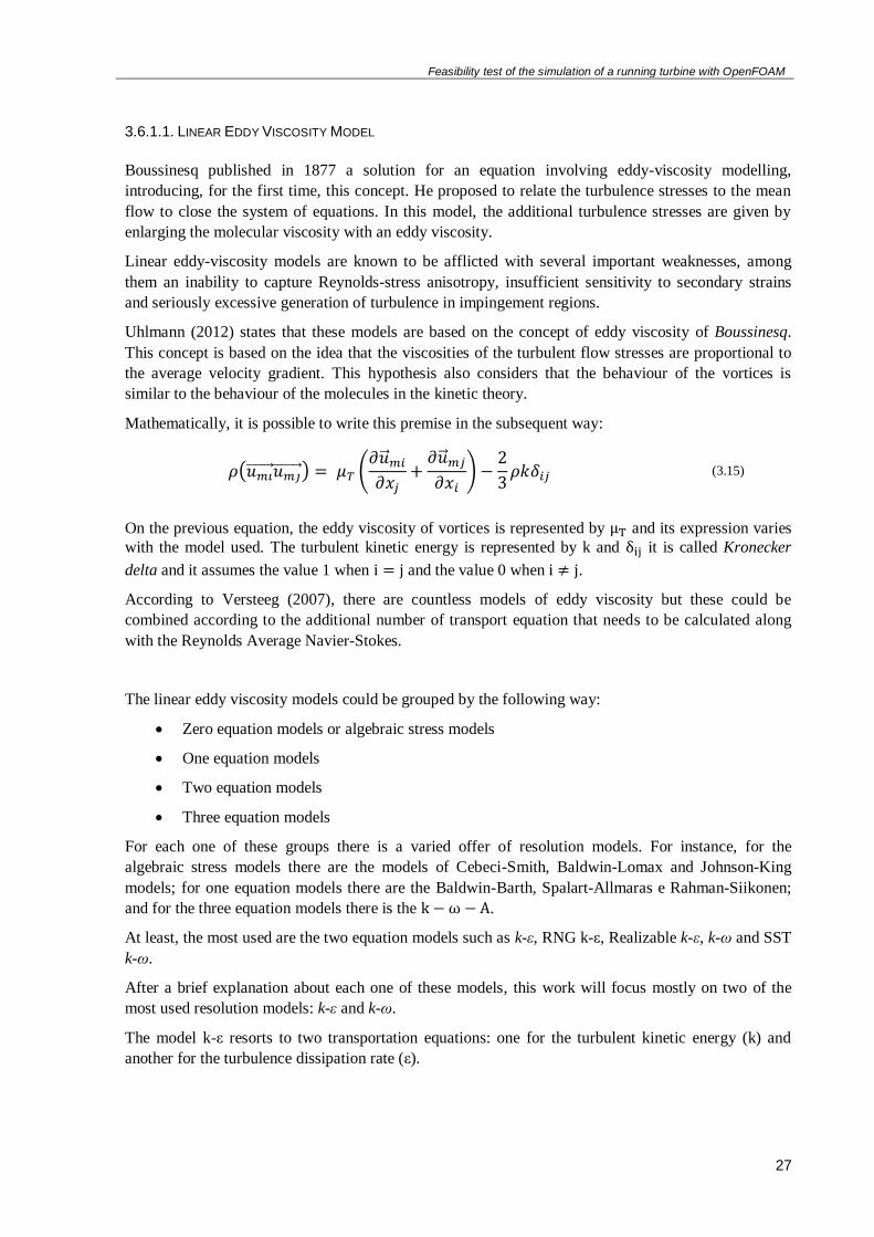
Mathematically, it is possible to write this premise in the subsequent way:
On the previous equation, the eddy viscosity of vortices is represented by μT and its expression varies
with the model used. The turbulent kinetic energy is represented by k and δij it is called Kronecker
delta and it assumes the value 1 when i = j and the value 0 when i ≠ j.
According to Versteeg (2007), there are countless models of eddy viscosity but these could be
combined according to the additional number of transport equation that needs to be calculated along
with the Reynolds Average Navier-Stokes.
The linear eddy viscosity models could be grouped by the following way:
Zero equation models or algebraic stress models
One equation models
Two equation models
Three equation models
For each one of these groups there is a varied offer of resolution models. For instance, for the
algebraic stress models there are the models of Cebeci-Smith, Baldwin-Lomax and Johnson-King
models; for one equation models there are the Baldwin-Barth, Spalart-Allmaras e Rahman-Siikonen;
and for the three equation models there is the k − ω − A.
At least, the most used are the two equation models such as k-ε, RNG k-ε, Realizable k-ε, k-ω and SST
k-ω.
After a brief explanation about each one of these models, this work will focus mostly on two of the
most used resolution models: k-ε and k-ω.
The model k-ε resorts to two transportation equations: one for the turbulent kinetic energy (k) and
another for the turbulence dissipation rate (ε).
𝜌(𝑢𝑚𝑖⃗⃗ ⃗⃗ ⃗⃗ 𝑢𝑚𝑗⃗⃗ ⃗⃗ ⃗⃗ ⃗) = 𝜇𝑇 (𝜕�⃗� 𝑚𝑖
𝜕𝑥𝑗+
𝜕�⃗� 𝑚𝑗
𝜕𝑥𝑖) −
2
3𝜌𝑘𝛿𝑖𝑗 (3.15)
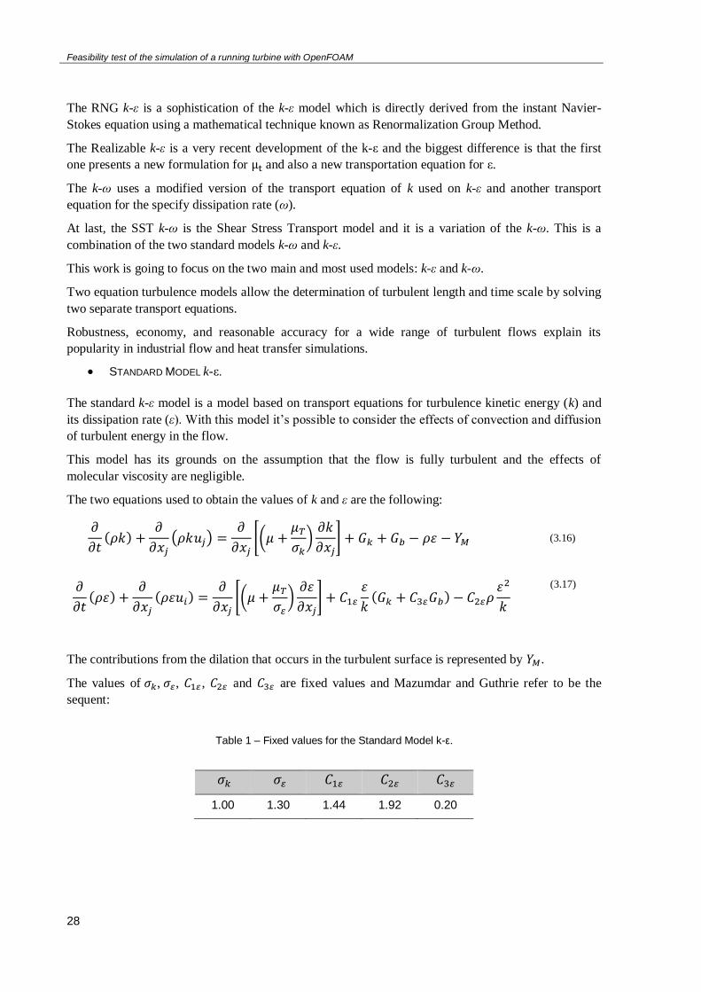
Feasibility test of the simulation of a running turbine with OpenFOAM
28
The RNG k-ε is a sophistication of the k-ε model which is directly derived from the instant Navier-
Stokes equation using a mathematical technique known as Renormalization Group Method.
The Realizable k-ε is a very recent development of the k-ε and the biggest difference is that the first
one presents a new formulation for μt and also a new transportation equation for ε.
The k-ω uses a modified version of the transport equation of k used on k-ε and another transport
equation for the specify dissipation rate (ω).
At last, the SST k-ω is the Shear Stress Transport model and it is a variation of the k-ω. This is a
combination of the two standard models k-ω and k-ε.
This work is going to focus on the two main and most used models: k-ε and k-ω.
Two equation turbulence models allow the determination of turbulent length and time scale by solving
two separate transport equations.
Robustness, economy, and reasonable accuracy for a wide range of turbulent flows explain its
popularity in industrial flow and heat transfer simulations.
STANDARD MODEL k-ε.
The standard k-ε model is a model based on transport equations for turbulence kinetic energy (k) and
its dissipation rate (ε). With this model it’s possible to consider the effects of convection and diffusion
of turbulent energy in the flow.
This model has its grounds on the assumption that the flow is fully turbulent and the effects of
molecular viscosity are negligible.
The two equations used to obtain the values of k and ε are the following:
The contributions from the dilation that occurs in the turbulent surface is represented by 𝑌𝑀.
The values of 𝜎𝑘, 𝜎𝜀, 𝐶1𝜀 , 𝐶2𝜀 and 𝐶3𝜀 are fixed values and Mazumdar and Guthrie refer to be the
sequent:
Table 1 – Fixed values for the Standard Model k-ε.
𝜎𝑘 𝜎𝜀 𝐶1𝜀 𝐶2𝜀 𝐶3𝜀
1.00 1.30 1.44 1.92 0.20
𝜕
𝜕𝑡(𝜌𝑘) +
𝜕
𝜕𝑥𝑗
(𝜌𝑘𝑢𝑗) =𝜕
𝜕𝑥𝑗
[(𝜇 +𝜇𝑇
𝜎𝑘)
𝜕𝑘
𝜕𝑥𝑗
] + 𝐺𝑘 + 𝐺𝑏 − 𝜌휀 − 𝑌𝑀 (3.16)
𝜕
𝜕𝑡(𝜌휀) +
𝜕
𝜕𝑥𝑗
(𝜌휀𝑢𝑖) =𝜕
𝜕𝑥𝑗
[(𝜇 +𝜇𝑇
𝜎𝜀)
𝜕휀
𝜕𝑥𝑗
] + 𝐶1𝜀
휀
𝑘(𝐺𝑘 + 𝐶3𝜀𝐺𝑏) − 𝐶2𝜀𝜌
휀2
𝑘
(3.17)
Feasibility test of the simulation of a running turbine with OpenFOAM
29
The generation of turbulent kinetic energy due to the average velocity gradient is represented by 𝐺𝑘
and can be calculated by:
Where S is the module of the average shear stress.
The turbulent kinetic energy generation due to boundary conditions is represented by 𝐺𝑏 and it’s
calculated by:
𝑃𝑟𝑡 is the Prandtl turbulent number for energy and its value is 0.85, g corresponds to the gravitational
component and the value of 𝜇𝑇 is calculated with the next equation presented:
According to Versteeg (2007), it is possible to translate the k-ε equations by this expression:
Rate of
change
of k or ε
+
Transport
of k or ε
by
convection
=
Transport
of k or ε
by
diffusion
+
Rate of
production
of k or ε
-
Rate of
destruction
of k or ε
To conclude, this model could be used for turbulent flows with free surface and interior flows
preferably with low pressure gradients. This model is highly discouraged to be used in flows with
separation of the boundary layer, rotating fluids, sudden changes in throttle rate and curved surfaces.
WILCOX MODEL k-ω.
The similarity of this model with the previous lays on the fact that both have a differential
equation for the variable of the turbulent kinetic energy k. The biggest difference is on the
second variable. In this model k-ω it is possible to calculate the energy dissipation rate
represented by ω. The value obtained when these equations are calculated represents the
turbulence scale which means that it represents the rate at which the energy dissipation occurs.
Relating the kinetic turbulent energy (k) with the energy dissipation (ε) and with the specific
dissipation rate (ω), Wilcox (1988) has proposed the following:
𝐺𝑘 = 𝜇𝑇𝑆2 (3.18)
𝐺𝑏 = −1
𝜌(𝜕𝜌
𝜕𝑇) × 𝑔 ×
𝜇𝑇
𝑃𝑟𝑡
𝜕𝑇
𝜕𝑥𝑖 (3.19)
𝜇𝑇 = ρCμ𝑘2
휀 (3.20)
ω =ε
Cμk (3.21)
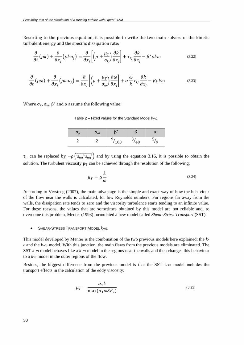
Feasibility test of the simulation of a running turbine with OpenFOAM
30
Resorting to the previous equation, it is possible to write the two main solvers of the kinetic
turbulent energy and the specific dissipation rate:
Where σk, σω, β∗ and α assume the following value:
Table 2 – Fixed values for the Standard Model k-ω.
𝜎𝑘 𝜎𝜔 β∗ β α
2 2 9100⁄ 3
40⁄ 59⁄
τij can be replaced by −ρ(umi′⃗⃗ ⃗⃗⃗⃗ ⃗⃗ umj′⃗⃗ ⃗⃗⃗⃗ ⃗⃗ ) and by using the equation 3.16, it is possible to obtain the
solution. The turbulent viscosity μT can be achieved through the resolution of the following:
According to Versteeg (2007), the main advantage is the simple and exact way of how the behaviour
of the flow near the walls is calculated, for low Reynolds numbers. For regions far away from the
walls, the dissipation rate tends to zero and the viscosity turbulence starts tending to an infinite value.
For these reasons, the values that are sometimes obtained by this model are not reliable and, to
overcome this problem, Menter (1993) formulated a new model called Shear-Stress Transport (SST).
SHEAR-STRESS TRANSPORT MODEL k-ω.
This model developed by Menter is the combination of the two previous models here explained: the k-
ε and the k-ω model. With this junction, the main flaws from the previous models are eliminated. The
SST k-ω model behaves like a k-ω model in the regions near the walls and then changes this behaviour
to a k-ε model in the outer regions of the flow.
Besides, the biggest difference from the previous model is that the SST k-ω model includes the
transport effects in the calculation of the eddy viscosity:
𝜇𝑇 =𝛼1𝑘
max (𝛼1𝜔𝑆𝐹2) (3.25)
𝜕
𝜕𝑡(𝜌𝑘) +
𝜕
𝜕𝑥𝑗
(𝜌𝑘𝑢𝑗) =𝜕
𝜕𝑥𝑗
[(𝜇 +𝜇𝑇
𝜎𝑘)
𝜕𝑘
𝜕𝑥𝑗
] + 𝜏𝑖𝑗
𝜕𝑘
𝜕𝑥𝑗− 𝛽∗𝜌𝑘𝜔 (3.22)
𝜕
𝜕𝑡(𝜌𝜔) +
𝜕
𝜕𝑥𝑗
(𝜌𝜔𝑢𝑗) =𝜕
𝜕𝑥𝑗
[(𝜇 +𝜇𝑇
𝜎𝜔)𝜕𝜔
𝜕𝑥𝑗
] + 𝛼𝜔
𝑘𝜏𝑖𝑗
𝜕𝑘
𝜕𝑥𝑗− 𝛽𝜌𝑘𝜔 (3.23)
𝜇𝑇 = ρ𝑘
𝜔 (3.24)
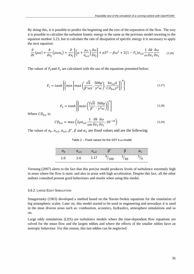
Feasibility test of the simulation of a running turbine with OpenFOAM
31
By doing this, it is possible to predict the beginning and the size of the separation of the flow. The way
it is possible to calculate the turbulent kinetic energy is the same as the previous model resorting to the
equation number 3.23, but to calculate the rate of dissipation of specific energy it is necessary to apply
the next equation:
𝜕
𝜕𝑡(𝜌𝜔) +
𝜕
𝜕𝑥𝑗(𝜌𝜔𝑢𝑗) =
𝜕
𝜕𝑥𝑗[(𝜇 +
𝜇𝑇
𝜎𝜔1)𝜕𝜔
𝜕𝑥𝑗] + 𝛼𝑆2 − 𝛽𝜔2 + 2(1 − 𝐹1)𝜎𝜔2
1
𝜔
𝜕𝑘
𝜕𝑥1
𝜕𝜔
𝜕𝑥1 (3.26)
The values of 𝐹1and 𝐹2 are calculated with the use of the equations presented below:
𝐹1 = 𝑡𝑎𝑛ℎ {{𝑚𝑖𝑛 [𝑚𝑎𝑥 (√𝑘
𝛽∗𝜔𝑦,500𝜇
𝑦2𝜔) ,
4𝜎𝜔2𝑘
𝐶𝐷𝑘𝜔𝑦2]}
4
} (3.27)
𝐹2 = 𝑡𝑎𝑛ℎ [[𝑚𝑎𝑥 (2√𝑘
𝛽∗,500𝜇
𝑦2𝜔)]
2
] (3.28)
Where 𝐶𝐷𝑘𝜔 is:
𝐶𝐷𝑘𝜔 = 𝑚𝑎𝑥 (2𝜌𝜎𝜔2
1
𝜔𝛼
𝜕𝑘
𝜕𝑥1
𝜕𝜔
𝜕𝑥1, 10−10) (3.29)
The values of 𝜎𝑘, 𝜎𝜔1, 𝜎𝜔2, 𝛽∗, 𝛽 and 𝛼1 are fixed values and are the following:
Table 2 – Fixed values for the SST k-ω model
𝜎𝑘 𝜎𝜔1 𝜎𝜔2 β∗ β α1
1.0 2.0 1.17 9100⁄ 3
40⁄ 59⁄
Versteeg (2007) alerts to the fact that this precise model produces levels of turbulence extremely high
in areas where the flow is static and also in areas with high acceleration. Despite this fact, all the other
authors consulted present good behaviours and results when using this model.
3.6.2. LARGE EDDY SIMULATION
Smagorinsky (1963) developed a method based on the Navier-Stokes equations for the simulation of
big atmospheric scales. Later on, this model started to be used in engineering and nowadays it is used
in the most diverse areas such as: combustion, acoustics, hydraulics, atmosphere simulations and so
on.
Large eddy simulations (LES) are turbulence models where the time-dependent flow equations are
solved for the mean flow and the largest eddies and where the effects of the smaller eddies have an
isotropic behaviour. For this reason, this last eddies can be neglected.
Feasibility test of the simulation of a running turbine with OpenFOAM
32
The LES model uses a space filtration to separate the smaller vortices from the big ones. During this
separation, the smaller ones get destroyed alloying the model to numerically obtain the behaviour of
the flow resorting to the Navier-Stokes equations for the highest dimensions movements.
𝜕𝑢1̅̅ ̅
𝜕𝑡+
𝜕
𝜕𝑥𝑗(𝑢𝑖𝑢�̅�̅̅ ̅̅ ̅) =
1
𝜌
𝜕�̅�
𝜕𝑥1+
𝜕
𝜕𝑥1(𝜇
𝜕𝑢1̅̅ ̅
𝜕𝑥𝑗) −
𝜕𝜏𝑖𝑗
𝜕𝑥1 (3.30)
Where �̅� and �̅� represent the velocity and pressure after filtration and 𝜏𝑖𝑗 is the residual stress it is
formulated depending on the sub models of mesh used.
According to Versteeg (2007), the LES model has a high precision regarding the calculation of the
Reynolds stress and the terms of transportation. With this precision, there is the need of a bigger
computational resolution and a much more fine mesh. The LES model needs the double of the
processing comparatively with the RANS model.
The need for a very fine mesh comes from the need that the simulations have to be addressed in such a
way that the vortex shear stresses are more tension relieved.
So that this can happen, filtering used cannot be larger than a small fraction of the fixed turbulent local
scale. This scale decreased as the wall approaches and with it the width of the filter.
When it comes to the resolution by the LES model, it should be noted that only a few years ago
computers began to have enough processing power to simulate flow by this method. (Versteeg. 2007)
3.6.3. DIRECT NUMERICAL SIMULATION
The direct numerical simulation (DNS) is based on the numerical modelling of flows through the
Navier-Stokes equations without any help or with the approach of turbulence models.
The full ranges of temporal and spatial turbulent scales have to be resolved, regardless of their size.
This means that in the direct numerical simulation, the smallest vortex and the fastest fluctuations are
settled, meaning that any movement, regardless of their irrelevance, is resolved.
The advantages of direct numerical simulation can be summarized in three points:
Extremely precise details and parameters of movement of turbulence at any point of the flow;
Instant results, which are not possible to get through experimentation, can be generated in
direct numerical simulation;
Modelling of turbulent flows that are impossible to happen in reality, for better physical
perception of this type of flow (eg walls without tensions).
Despite these advantages, direct numerical simulation is almost exclusively applied to research and at
low Reynolds numbers.
The fact that all the parameters are thoroughly modelled results in a very time-consuming and costly
numerical modelling (Versteeg. 2007).
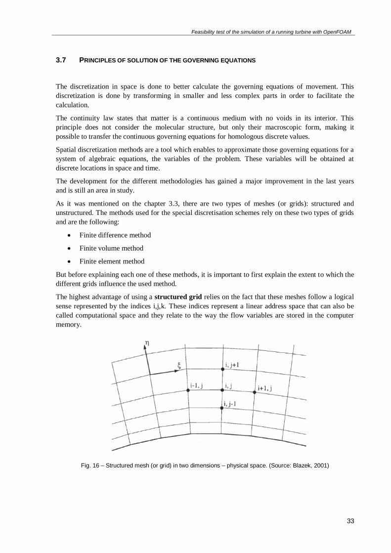
Feasibility test of the simulation of a running turbine with OpenFOAM
33
3.7 PRINCIPLES OF SOLUTION OF THE GOVERNING EQUATIONS
The discretization in space is done to better calculate the governing equations of movement. This
discretization is done by transforming in smaller and less complex parts in order to facilitate the
calculation.
The continuity law states that matter is a continuous medium with no voids in its interior. This
principle does not consider the molecular structure, but only their macroscopic form, making it
possible to transfer the continuous governing equations for homologous discrete values.
Spatial discretization methods are a tool which enables to approximate those governing equations for a
system of algebraic equations, the variables of the problem. These variables will be obtained at
discrete locations in space and time.
The development for the different methodologies has gained a major improvement in the last years
and is still an area in study.
As it was mentioned on the chapter 3.3, there are two types of meshes (or grids): structured and
unstructured. The methods used for the special discretisation schemes rely on these two types of grids
and are the following:
Finite difference method
Finite volume method
Finite element method
But before explaining each one of these methods, it is important to first explain the extent to which the
different grids influence the used method.
The highest advantage of using a structured grid relies on the fact that these meshes follow a logical
sense represented by the indices i,j,k. These indices represent a linear address space that can also be
called computational space and they relate to the way the flow variables are stored in the computer
memory.
Fig. 16 – Structured mesh (or grid) in two dimensions – physical space. (Source: Blazek, 2001)
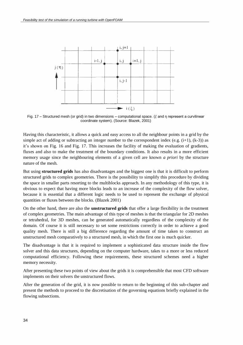
Feasibility test of the simulation of a running turbine with OpenFOAM
34
Fig. 17 – Structured mesh (or grid) in two dimensions – computational space. (𝜉 and η represent a curvilinear
coordinate system). (Source: Blazek, 2001)
Having this characteristic, it allows a quick and easy access to all the neighbour points in a grid by the
simple act of adding or subtracting an integer number to the correspondent index (e.g. (i+1), (k-3)) as
it’s shown on Fig. 16 and Fig. 17. This increases the facility of making the evaluation of gradients,
fluxes and also to make the treatment of the boundary conditions. It also results in a more efficient
memory usage since the neighbouring elements of a given cell are known a priori by the structure
nature of the mesh.
But using structured grids has also disadvantages and the biggest one is that it is difficult to perform
structured grids to complex geometries. There is the possibility to simplify this procedure by dividing
the space in smaller parts resorting to the multiblocks approach. In any methodology of this type, it is
obvious to expect that having more blocks leads to an increase of the complexity of the flow solver,
because it is essential that a different logic needs to be used to represent the exchange of physical
quantities or fluxes between the blocks. (Blazek 2001)
On the other hand, there are also the unstructured grids that offer a large flexibility in the treatment
of complex geometries. The main advantage of this type of meshes is that the triangular for 2D meshes
or tetrahedral, for 3D meshes, can be generated automatically regardless of the complexity of the
domain. Of course it is still necessary to set some restrictions correctly in order to achieve a good
quality mesh. There is still a big difference regarding the amount of time taken to construct an
unstructured mesh comparatively to a structured mesh, in which the first one is much quicker.
The disadvantage is that it is required to implement a sophisticated data structure inside the flow
solver and this data structures, depending on the computer hardware, takes to a more or less reduced
computational efficiency. Following these requirements, these structured schemes need a higher
memory necessity.
After presenting these two points of view about the grids it is comprehensible that most CFD software
implements on their solvers the unstructured flows.
After the generation of the grid, it is now possible to return to the beginning of this sub-chapter and
present the methods to proceed to the discretisation of the governing equations briefly explained in the
flowing subsections.
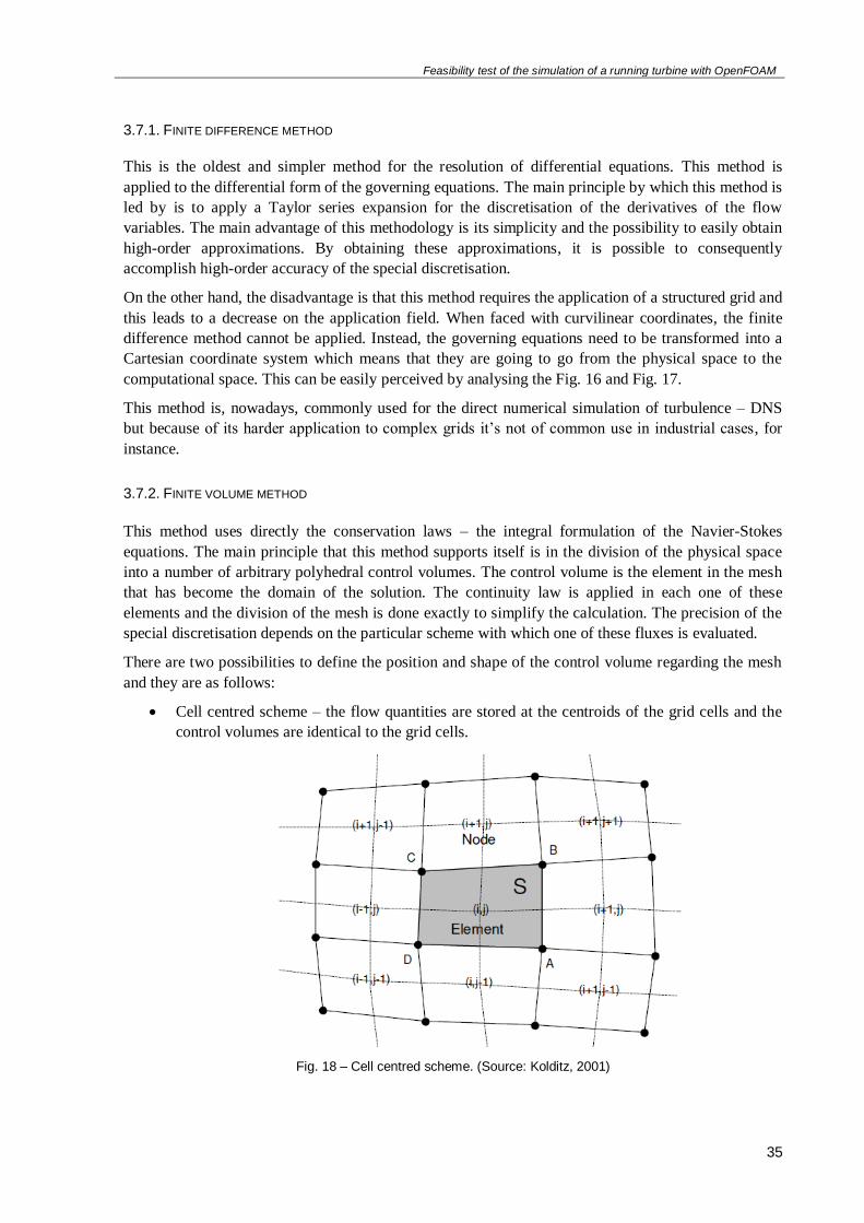
Feasibility test of the simulation of a running turbine with OpenFOAM
35
3.7.1. FINITE DIFFERENCE METHOD
This is the oldest and simpler method for the resolution of differential equations. This method is
applied to the differential form of the governing equations. The main principle by which this method is
led by is to apply a Taylor series expansion for the discretisation of the derivatives of the flow
variables. The main advantage of this methodology is its simplicity and the possibility to easily obtain
high-order approximations. By obtaining these approximations, it is possible to consequently
accomplish high-order accuracy of the special discretisation.
On the other hand, the disadvantage is that this method requires the application of a structured grid and
this leads to a decrease on the application field. When faced with curvilinear coordinates, the finite
difference method cannot be applied. Instead, the governing equations need to be transformed into a
Cartesian coordinate system which means that they are going to go from the physical space to the
computational space. This can be easily perceived by analysing the Fig. 16 and Fig. 17.
This method is, nowadays, commonly used for the direct numerical simulation of turbulence – DNS
but because of its harder application to complex grids it’s not of common use in industrial cases, for
instance.
3.7.2. FINITE VOLUME METHOD
This method uses directly the conservation laws – the integral formulation of the Navier-Stokes
equations. The main principle that this method supports itself is in the division of the physical space
into a number of arbitrary polyhedral control volumes. The control volume is the element in the mesh
that has become the domain of the solution. The continuity law is applied in each one of these
elements and the division of the mesh is done exactly to simplify the calculation. The precision of the
special discretisation depends on the particular scheme with which one of these fluxes is evaluated.
There are two possibilities to define the position and shape of the control volume regarding the mesh
and they are as follows:
Cell centred scheme – the flow quantities are stored at the centroids of the grid cells and the
control volumes are identical to the grid cells.
Fig. 18 – Cell centred scheme. (Source: Kolditz, 2001)
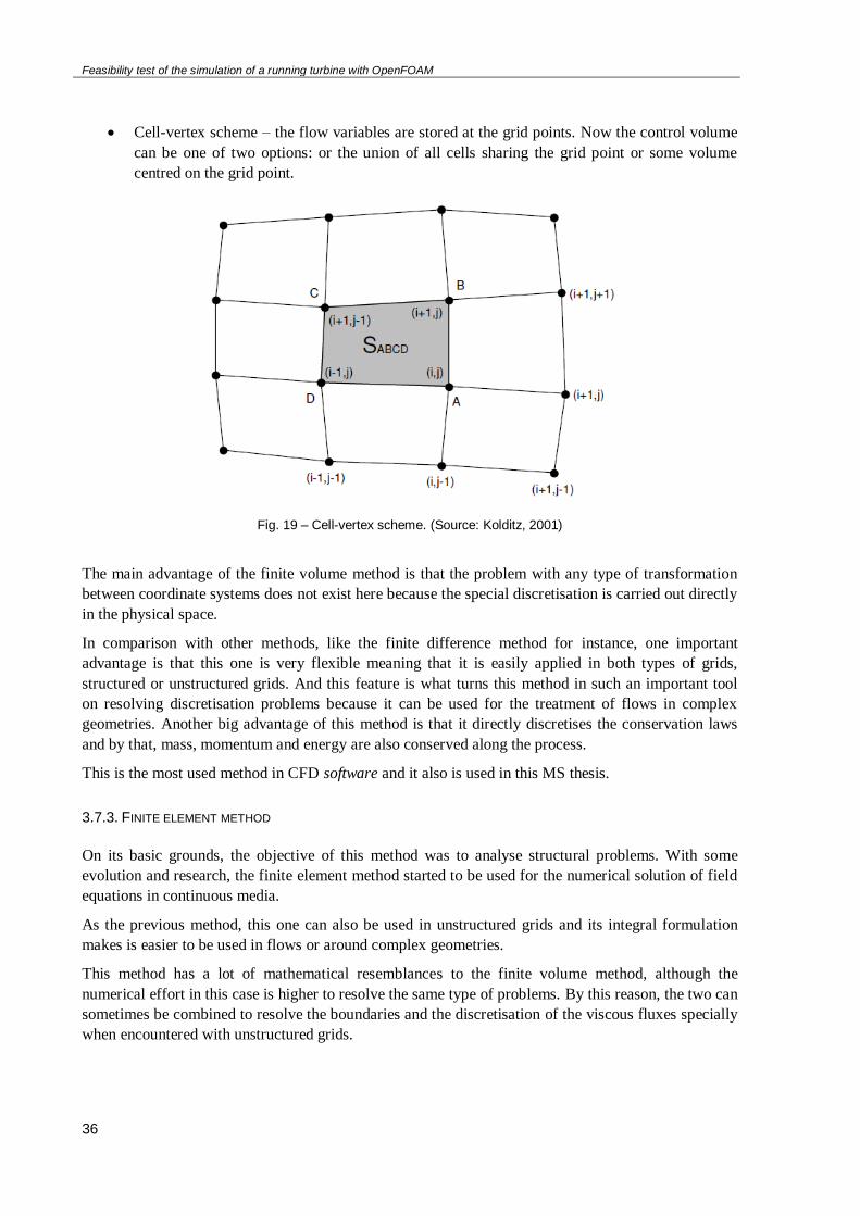
Feasibility test of the simulation of a running turbine with OpenFOAM
36
Cell-vertex scheme – the flow variables are stored at the grid points. Now the control volume
can be one of two options: or the union of all cells sharing the grid point or some volume
centred on the grid point.
Fig. 19 – Cell-vertex scheme. (Source: Kolditz, 2001)
The main advantage of the finite volume method is that the problem with any type of transformation
between coordinate systems does not exist here because the special discretisation is carried out directly
in the physical space.
In comparison with other methods, like the finite difference method for instance, one important
advantage is that this one is very flexible meaning that it is easily applied in both types of grids,
structured or unstructured grids. And this feature is what turns this method in such an important tool
on resolving discretisation problems because it can be used for the treatment of flows in complex
geometries. Another big advantage of this method is that it directly discretises the conservation laws
and by that, mass, momentum and energy are also conserved along the process.
This is the most used method in CFD software and it also is used in this MS thesis.
3.7.3. FINITE ELEMENT METHOD
On its basic grounds, the objective of this method was to analyse structural problems. With some
evolution and research, the finite element method started to be used for the numerical solution of field
equations in continuous media.
As the previous method, this one can also be used in unstructured grids and its integral formulation
makes is easier to be used in flows or around complex geometries.
This method has a lot of mathematical resemblances to the finite volume method, although the
numerical effort in this case is higher to resolve the same type of problems. By this reason, the two can
sometimes be combined to resolve the boundaries and the discretisation of the viscous fluxes specially
when encountered with unstructured grids.
Feasibility test of the simulation of a running turbine with OpenFOAM
37
4 Computational Fluid Dynamics –
Procedure
4.1. DESCRIPTION OF THE MODEL
The main objective of this work was to validate the possibility of building a numerical model of a
running turbine in the software OpenFOAM. Most of the studies, so far, were based on probabilities of
occurrence of fish injury and achieving the result with this software could be a support for validation
of the existing models.
Most of the numerical studies made so far were accomplished resorting to Propeller turbines like
Kaplan and Francis turbines and ,by that fact, the simulation developed in this project will be made
with a four blade propeller turbine.
An exact model of a complete turbine with all its components would be very extensive for the time
available to perform this work and by this it was chosen to generate the part of the turbine that has
movement: its rotor and the respective blades. It was also defined a box where the turbine was inserted
that afterwards would have an inflow.
This model allows a better comprehension of the values of velocity and pressure while the turbine is in
movement.
4.2. PROCEDURE
As any CFD analysis, the major point is to obtain a deeper understanding of the problem under
consideration and to have valid results, the need to make appropriate choices when it comes to the
solver applications is also required.
In every computational fluid dynamics, the basic steps are usually common, regardless the software in
question. In this work, making use of the OpenFOAM software, the mandatory steps followed were:
1. Problem definition
2. Pre-processing and mesh generation
3. Choice of turbulence model
4. Selection of boundary conditions
5. Selection of the solver
6. Execution of the numeric study
7. Discussion and verification of the results
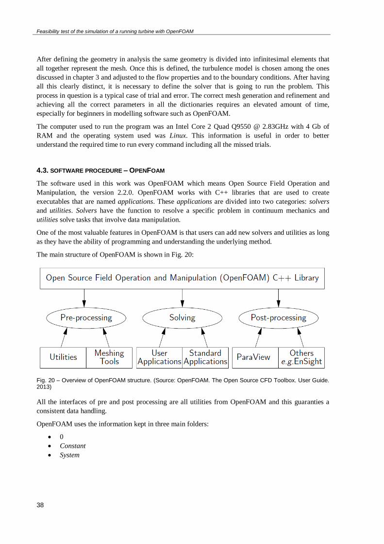
Feasibility test of the simulation of a running turbine with OpenFOAM
38
After defining the geometry in analysis the same geometry is divided into infinitesimal elements that
all together represent the mesh. Once this is defined, the turbulence model is chosen among the ones
discussed in chapter 3 and adjusted to the flow properties and to the boundary conditions. After having
all this clearly distinct, it is necessary to define the solver that is going to run the problem. This
process in question is a typical case of trial and error. The correct mesh generation and refinement and
achieving all the correct parameters in all the dictionaries requires an elevated amount of time,
especially for beginners in modelling software such as OpenFOAM.
The computer used to run the program was an Intel Core 2 Quad Q9550 @ 2.83GHz with 4 Gb of
RAM and the operating system used was Linux. This information is useful in order to better
understand the required time to run every command including all the missed trials.
4.3. SOFTWARE PROCEDURE – OPENFOAM
The software used in this work was OpenFOAM which means Open Source Field Operation and
Manipulation, the version 2.2.0. OpenFOAM works with C++ libraries that are used to create
executables that are named applications. These applications are divided into two categories: solvers
and utilities. Solvers have the function to resolve a specific problem in continuum mechanics and
utilities solve tasks that involve data manipulation.
One of the most valuable features in OpenFOAM is that users can add new solvers and utilities as long
as they have the ability of programming and understanding the underlying method.
The main structure of OpenFOAM is shown in Fig. 20:
Fig. 20 – Overview of OpenFOAM structure. (Source: OpenFOAM. The Open Source CFD Toolbox. User Guide. 2013)
All the interfaces of pre and post processing are all utilities from OpenFOAM and this guaranties a
consistent data handling.
OpenFOAM uses the information kept in three main folders:
0
Constant
System
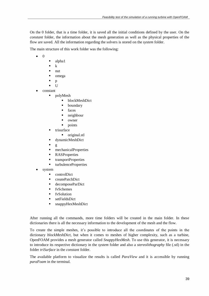
Feasibility test of the simulation of a running turbine with OpenFOAM
39
On the 0 folder, that is a time folder, it is saved all the initial conditions defined by the user. On the
constant folder, the information about the mesh generation as well as the physical properties of the
flow are saved. All the information regarding the solvers is stored on the system folder.
The main structure of this work folder was the following:
0
alpha1
k
nut
omega
p
U
constant
polyMesh
blockMeshDict
boundary
faces
neighbour
owner
points
trisurface
original.stl
dynamicMeshDict
g
mechanicalProperties
RASProperties
transportProperties
turbulenceProperties
system
controlDict
createPatchDict
decomposeParDict
fvSchemes
fvSolution
setFieldsDict
snappyHexMeshDict
After running all the commands, more time folders will be created in the main folder. In these
dictionaries there is all the necessary information to the development of the mesh and the flow.
To create the simple meshes, it’s possible to introduce all the coordinates of the points in the
dictionary blockMeshDict, but when it comes to meshes of higher complexity, such as a turbine,
OpenFOAM provides a mesh generator called SnappyHexMesh. To use this generator, it is necessary
to introduce its respective dictionary in the system folder and also a stereolithography file (.stl) in the
folder triSurface in the constant folder.
The available platform to visualize the results is called ParaView and it is accessible by running
paraFoam in the terminal.
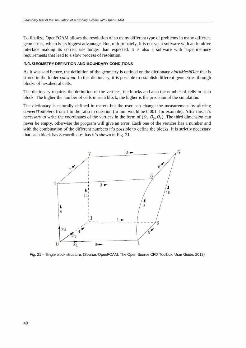
Feasibility test of the simulation of a running turbine with OpenFOAM
40
To finalize, OpenFOAM allows the resolution of so many different type of problems in many different
geometries, which is its biggest advantage. But, unfortunately, it is not yet a software with an intuitive
interface making its correct use longer than expected. It is also a software with large memory
requirements that lead to a slow process of resolution.
4.4. GEOMETRY DEFINITION AND BOUNDARY CONDITIONS
As it was said before, the definition of the geometry is defined on the dictionary blockMeshDict that is
stored in the folder constant. In this dictionary, it is possible to establish different geometries through
blocks of hexahedral cells.
The dictionary requires the definition of the vertices, the blocks and also the number of cells in each
block. The higher the number of cells in each block, the higher is the precision of the simulation.
The dictionary is naturally defined in meters but the user can change the measurement by altering
convertToMeters from 1 to the ratio in question (to mm would be 0.001, for example). After this, it’s
necessary to write the coordinates of the vertices in the form of (𝑂𝑥 , 𝑂𝑦 , 𝑂𝑧). The third dimension can
never be empty, otherwise the program will give an error. Each one of the vertices has a number and
with the combination of the different numbers it’s possible to define the blocks. It is strictly necessary
that each block has 8 coordinates has it’s shown in Fig. 21.
Fig. 21 – Single block structure. (Source: OpenFOAM. The Open Source CFD Toolbox, User Guide, 2013)
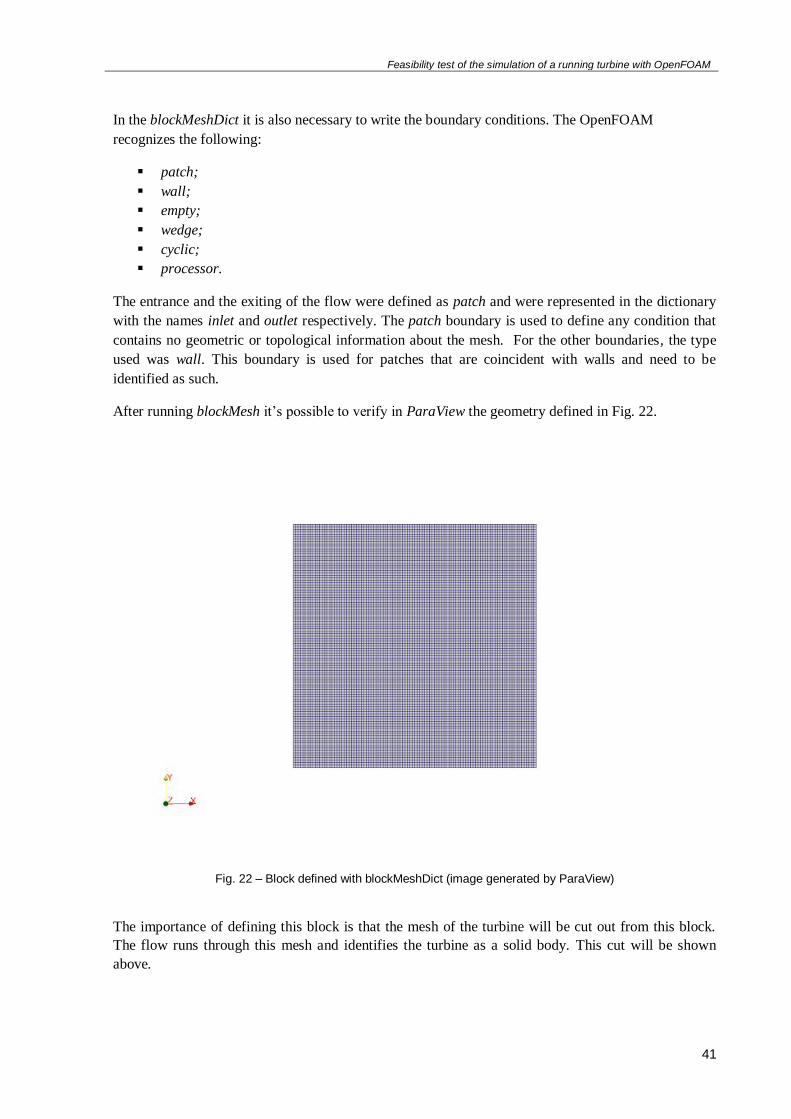
Feasibility test of the simulation of a running turbine with OpenFOAM
41
In the blockMeshDict it is also necessary to write the boundary conditions. The OpenFOAM
recognizes the following:
patch;
wall;
empty;
wedge;
cyclic;
processor.
The entrance and the exiting of the flow were defined as patch and were represented in the dictionary
with the names inlet and outlet respectively. The patch boundary is used to define any condition that
contains no geometric or topological information about the mesh. For the other boundaries, the type
used was wall. This boundary is used for patches that are coincident with walls and need to be
identified as such.
After running blockMesh it’s possible to verify in ParaView the geometry defined in Fig. 22.
Fig. 22 – Block defined with blockMeshDict (image generated by ParaView)
The importance of defining this block is that the mesh of the turbine will be cut out from this block.
The flow runs through this mesh and identifies the turbine as a solid body. This cut will be shown
above.
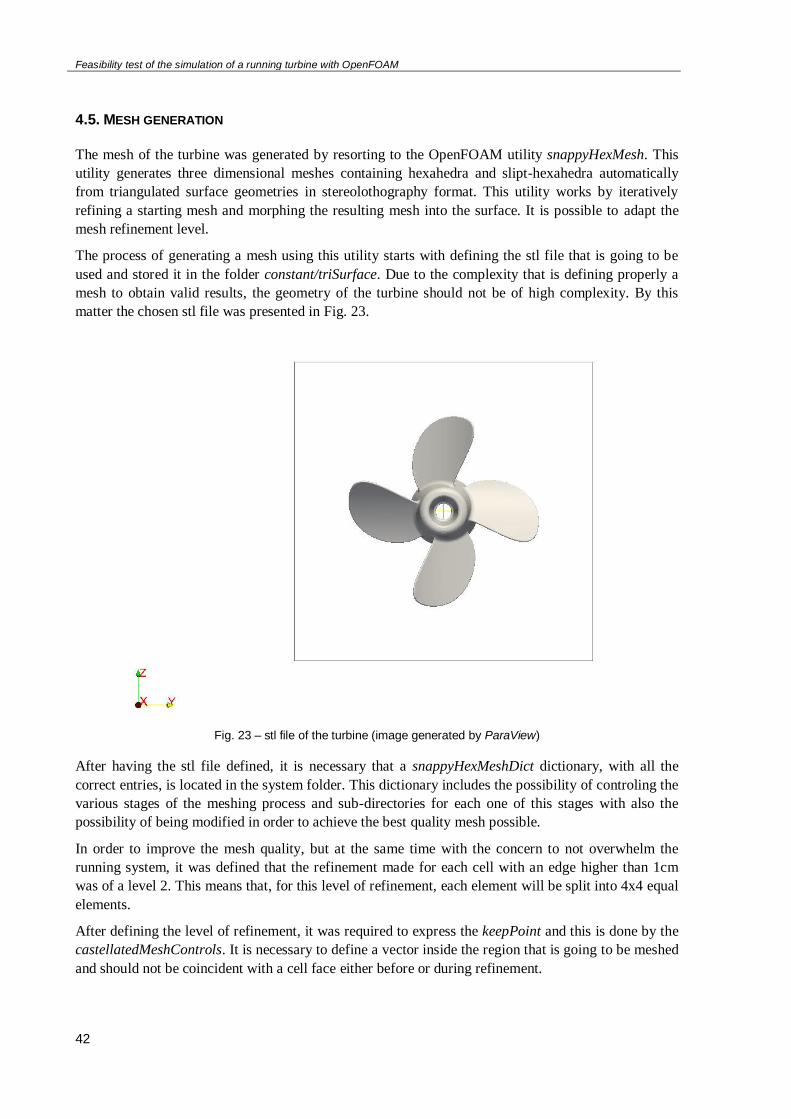
Feasibility test of the simulation of a running turbine with OpenFOAM
42
4.5. MESH GENERATION
The mesh of the turbine was generated by resorting to the OpenFOAM utility snappyHexMesh. This
utility generates three dimensional meshes containing hexahedra and slipt-hexahedra automatically
from triangulated surface geometries in stereolothography format. This utility works by iteratively
refining a starting mesh and morphing the resulting mesh into the surface. It is possible to adapt the
mesh refinement level.
The process of generating a mesh using this utility starts with defining the stl file that is going to be
used and stored it in the folder constant/triSurface. Due to the complexity that is defining properly a
mesh to obtain valid results, the geometry of the turbine should not be of high complexity. By this
matter the chosen stl file was presented in Fig. 23.
Fig. 23 – stl file of the turbine (image generated by ParaView)
After having the stl file defined, it is necessary that a snappyHexMeshDict dictionary, with all the
correct entries, is located in the system folder. This dictionary includes the possibility of controling the
various stages of the meshing process and sub-directories for each one of this stages with also the
possibility of being modified in order to achieve the best quality mesh possible.
In order to improve the mesh quality, but at the same time with the concern to not overwhelm the
running system, it was defined that the refinement made for each cell with an edge higher than 1cm
was of a level 2. This means that, for this level of refinement, each element will be split into 4x4 equal
elements.
After defining the level of refinement, it was required to express the keepPoint and this is done by the
castellatedMeshControls. It is necessary to define a vector inside the region that is going to be meshed
and should not be coincident with a cell face either before or during refinement.
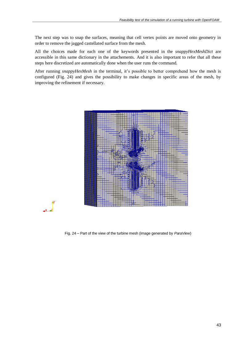
Feasibility test of the simulation of a running turbine with OpenFOAM
43
The next step was to snap the surfaces, meaning that cell vertex points are moved onto geometry in
order to remove the jagged castellated surface from the mesh.
All the choices made for each one of the keywords presented in the snappyHexMeshDict are
accessible in this same dictionary in the attachements. And it is also important to refer that all these
steps here discretized are automatically done when the user runs the command.
After running snappyHexMesh in the terminal, it’s possible to better comprehend how the mesh is
configured (Fig. 24) and gives the possibility to make changes in specific areas of the mesh, by
improving the refinement if necessary.
Fig. 24 – Part of the view of the turbine mesh (image generated by ParaView)
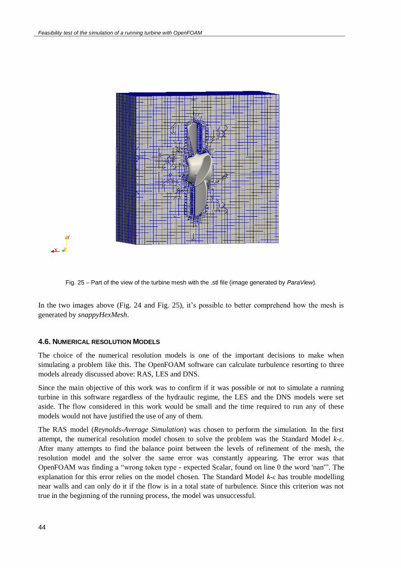
Feasibility test of the simulation of a running turbine with OpenFOAM
44
Fig. 25 – Part of the view of the turbine mesh with the .stl file (image generated by ParaView).
In the two images above (Fig. 24 and Fig. 25), it’s possible to better comprehend how the mesh is
generated by snappyHexMesh.
4.6. NUMERICAL RESOLUTION MODELS
The choice of the numerical resolution models is one of the important decisions to make when
simulating a problem like this. The OpenFOAM software can calculate turbulence resorting to three
models already discussed above: RAS, LES and DNS.
Since the main objective of this work was to confirm if it was possible or not to simulate a running
turbine in this software regardless of the hydraulic regime, the LES and the DNS models were set
aside. The flow considered in this work would be small and the time required to run any of these
models would not have justified the use of any of them.
The RAS model (Reynolds-Average Simulation) was chosen to perform the simulation. In the first
attempt, the numerical resolution model chosen to solve the problem was the Standard Model k-ε.
After many attempts to find the balance point between the levels of refinement of the mesh, the
resolution model and the solver the same error was constantly appearing. The error was that
OpenFOAM was finding a “wrong token type - expected Scalar, found on line 0 the word 'nan'”. The
explanation for this error relies on the model chosen. The Standard Model k-ε has trouble modelling
near walls and can only do it if the flow is in a total state of turbulence. Since this criterion was not
true in the beginning of the running process, the model was unsuccessful.
Feasibility test of the simulation of a running turbine with OpenFOAM
45
After this trial and error, the resolution model was changed to the Shear-Stress Transport Model k-ω.
This is a more ample model that is not that affected by the mesh in study or the flow properties.
In the folder constant there is the dictionary needed to state all the choices, regarding the resolution
model. In the turbulenceProperties dictionary, it’s necessary to define the RAS model and after that,
in the RASProperties dictionary, it was chosen the SST k-ω method.
4.7. INITIAL CONDITIONS
All the initial conditions that the program had to take into account before the beginning of the
simulation are in the 0 folder. Each one of the dictionaries presented in this folder characterizes one of
the properties that the user wants to see in the simulation.
alpha1;
nut;
U ;
k ;
p ;
omega;
In the dictionary alpha1 is where it’s possible to define the cells where the flow is. It’s given the value
1 to the cells where the water should be and 0 to the cells where it shouldn’t. It was defined on the
patch inlet the only inflow and was given the value 0 to all the other boundaries. The characteristics of
the walls were defined in the nut dictionary, the velocity in the U dictionary and the turbulent kinetic
energy in the k dictionary. The pressure is defined in the p dictionary and depending on the type of the
resolution model it can be used the omega or the epsilon model.
4.8. DEFINITION OF THE MOVEMENT OF THE TURBINE
If proceeding simulations in OpenFOAM with steady grids could be difficult, with dynamic meshes
it’s definitely challenging. The functionalities available to improve movement in OpenFOAM
software include solid body motion of a mesh according to the defined motion function, internal
motion like distortion among other that are calculated from boundary motion, dynamic refinement and
unrefinement of hexahedral meshes and prescribed motion of the mesh.
4.8.1. FIRST APPROACH RESORTING TO ANGULAROSCILLATINGVELOCITY
To begin the process of inducing movement to the turbine was added to the folder 0 the dictionaries
pointMotionU and cellMotionU. Both of them contain the input values that control the movement of
the oscillating patch, in this case: turbine_path28539.
After the definition of these two dictionaries, it was also required to change the fvschemes and the
fvsolutions and finally the motion solver.
The OpenFOAM software provides two libraries that can produce the oscillation of the patches. They
are called angularOscillatingVelocity and angularOscilatingDisplacement. In this work it’s the
angularOscillatingVelocity that is going to be used. With this function, the velocity of each point is
calculated for each time step.
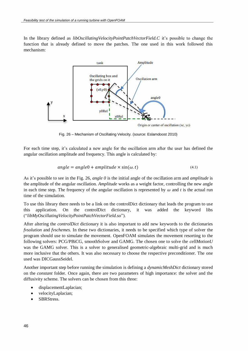
Feasibility test of the simulation of a running turbine with OpenFOAM
46
In the library defined as libOscillatingVelocityPointPatchVectorField.C it’s possible to change the
function that is already defined to move the patches. The one used in this work followed this
mechanism:
Fig. 26 – Mechanism of Oscillating Velocity. (source: Eslamdoost 2010)
For each time step, it’s calculated a new angle for the oscillation arm after the user has defined the
angular oscillation amplitude and frequency. This angle is calculated by:
𝑎𝑛𝑔𝑙𝑒 = 𝑎𝑛𝑔𝑙𝑒0 + 𝑎𝑚𝑝𝑙𝑖𝑡𝑢𝑑𝑒 × sin (𝜔. 𝑡) (4.1)
As it’s possible to see in the Fig. 26, angle 0 is the initial angle of the oscillation arm and amplitude is
the amplitude of the angular oscillation. Amplitude works as a weight factor, controlling the new angle
in each time step. The frequency of the angular oscillation is represented by 𝜔 and t is the actual run
time of the simulation.
To use this library there needs to be a link on the controlDict dictionary that leads the program to use
this application. On the controlDict dictionary, it was added the keyword libs
(“libMyOscillatingVelocityPointPatchVectorField.so”).
After altering the controlDict dictionary it is also important to add new keywords to the dictionaries
fvsolution and fvschemes. In these two dictionaries, it needs to be specified which type of solver the
program should use to simulate the movement. OpenFOAM simulates the movement resorting to the
following solvers: PCG/PBiCG, smoothSolver and GAMG. The chosen one to solve the cellMotionU
was the GAMG solver. This is a solver to generalised geometric-algebraic multi-grid and is much
more inclusive that the others. It was also necessary to choose the respective preconditioner. The one
used was DICGaussSeidel.
Another important step before running the simulation is defining a dynamicMeshDict dictionary stored
on the constant folder. Once again, there are two parameters of high importance: the solver and the
diffusivity scheme. The solvers can be chosen from this three:
displacementLaplacian;
velocityLaplacian;
SBRStress.
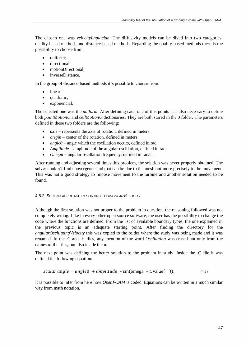
Feasibility test of the simulation of a running turbine with OpenFOAM
47
The chosen one was velocityLaplacian. The diffusivity models can be dived into two categories:
quality-based methods and distance-based methods. Regarding the quality-based methods there is the
possibility to choose from:
uniform;
directional;
motionDirectional;
inverseDistance.
In the group of distance-based methods it’s possible to choose from:
linear;
quadratic;
exponencial.
The selected one was the uniform. After defining each one of this points it is also necessary to define
both pointMotionU and cellMotionU dictionaries. They are both stored in the 0 folder. The parameters
defined in these two folders are the following:
axis – represents the axis of rotation, defined in meters.
origin – center of the rotation, defined in meters.
angle0 – angle which the oscillation occurs, defined in rad.
Amplitude – amplitude of the angular oscillation, defined in rad.
Omega – angular oscillation frequency, defined in rad/s.
After running and adjusting several times this problem, the solution was never properly obtained. The
solver couldn’t find convergence and that can be due to the mesh but more precisely to the movement.
This was not a good strategy to impose movement to the turbine and another solution needed to be
found.
4.8.2. SECOND APPROACH RESORTING TO ANGULARVELOCITY
Although the first solution was not proper to the problem in question, the reasoning followed was not
completely wrong. Like in every other open source software, the user has the possibility to change the
code where the functions are defined. From the list of available boundary types, the one explained in
the previous topic is an adequate starting point. After finding the directory for the
angularOscillatingVelocity this was copied to the folder where the study was being made and it was
renamed. In the .C and .H files, any mention of the word Oscillating was erased not only from the
names of the files, but also inside them.
The next point was defining the better solution to the problem in study. Inside the .C file it was
defined the following equation:
𝑠𝑐𝑎𝑙𝑎𝑟 𝑎𝑛𝑔𝑙𝑒 = 𝑎𝑛𝑔𝑙𝑒0_ + 𝑎𝑚𝑝𝑙𝑖𝑡𝑢𝑑e_ ∗ sin (omega_ ∗ 𝑡. value( )); (4.2)
It is possible to infer from here how OpenFOAM is coded. Equations can be written in a much similar
way from math notation.

Feasibility test of the simulation of a running turbine with OpenFOAM
48
This is where modification should be done in order to obtain the desired movement. The new equation
is:
𝑠𝑐𝑎𝑙𝑎𝑟 𝑎𝑛𝑔𝑙𝑒 = 𝑎𝑛𝑔𝑙𝑒0_ + omega_ ∗ 𝑡. value( ); (4.3)
The amplitude and the sin function were eliminated. In the two files .C and .H all the lines of code
where the word amplitude appears were eliminated as well.
After this was defined, the compilation of the parameters was determined. The files file inside the
Make directory changed into:
angularVelocity/angularVelocityPointPatchVectorField.C
LIB = $(FOAM_USER_LIBBIN)/libAngularVelocityPointPatchVectorField
The first line leads to the location of the .C file with the source code and the second to the directory
where user libraries for OpenFOAM are stored followed by the name of the library that was created.
Once all the files were correctly defined, it was necessary to compile the library by running:
wmake libso
After this new library was created, there is the need to define in the controlDic dictionary the path
where the program needs to find the new code to solve the problem. So, in this dictionary, it is added:
Libs (“libAngularVelocityPointPatchVectorField.so” “libOpenFOAM.so”)
After this library is defined, the boundaries in the dictionaries pointMotionU needs to be corrected
according to the new library created. The important part of this library is the part where the boundary
of the turbine is defined and it’s the following:
turbine_patch28539
{
type libAngularVelocity;
axis (1 0 0);
origin (0 0 0);
angle0 0;
omega 20.94; //200rpm
value uniform (1 0 0);
}
A propeller turbine can go from 79 rpm to 429 rpm. Since this is a numerical study, an intermediate
value was chosen: 200rpm that correspond to 20.94 rad/s.
Before running the problem, it is important to verify if the mesh is well constructed and so it’s
necessary to run checkMesh. The log file that is acquired when running this is in the appendix E.
Due to the high computational requisitions of the software, it was used the decomposePar tool that
divides the main processor into 8 smaller processors and by that it is possible to achieve quicker
results. Nevertheless, attention must be taken when doing this because a lot of boundary conditions
may not be correctly handled and the user needs to correct them manually.
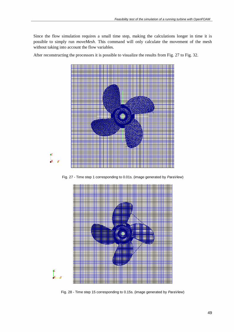
Feasibility test of the simulation of a running turbine with OpenFOAM
49
Since the flow simulation requires a small time step, making the calculations longer in time it is
possible to simply run moveMesh. This command will only calculate the movement of the mesh
without taking into account the flow variables.
After reconstructing the processors it is possible to visualize the results from Fig. 27 to Fig. 32.
Fig. 27 - Time step 1 corresponding to 0.01s. (image generated by ParaView)
Fig. 28 - Time step 15 corresponding to 0.15s. (image generated by ParaView)

Feasibility test of the simulation of a running turbine with OpenFOAM
50
Fig. 29 - Time step 100 corresponding to 1s. (image generated by ParaView)
Fig. 30 - Time step 200 corresponding to 2s. (image generated by ParaView)
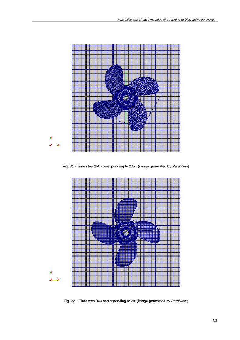
Feasibility test of the simulation of a running turbine with OpenFOAM
51
Fig. 31 - Time step 250 corresponding to 2.5s. (image generated by ParaView)
Fig. 32 – Time step 300 corresponding to 3s. (image generated by ParaView)
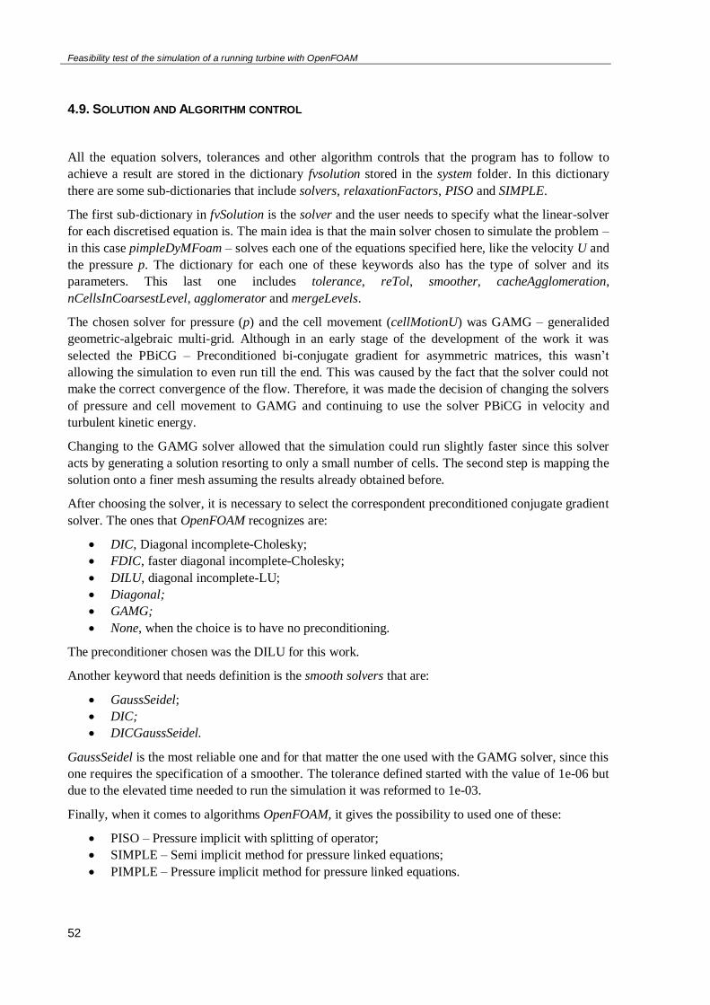
Feasibility test of the simulation of a running turbine with OpenFOAM
52
4.9. SOLUTION AND ALGORITHM CONTROL
All the equation solvers, tolerances and other algorithm controls that the program has to follow to
achieve a result are stored in the dictionary fvsolution stored in the system folder. In this dictionary
there are some sub-dictionaries that include solvers, relaxationFactors, PISO and SIMPLE.
The first sub-dictionary in fvSolution is the solver and the user needs to specify what the linear-solver
for each discretised equation is. The main idea is that the main solver chosen to simulate the problem –
in this case pimpleDyMFoam – solves each one of the equations specified here, like the velocity U and
the pressure p. The dictionary for each one of these keywords also has the type of solver and its
parameters. This last one includes tolerance, reTol, smoother, cacheAgglomeration,
nCellsInCoarsestLevel, agglomerator and mergeLevels.
The chosen solver for pressure (p) and the cell movement (cellMotionU) was GAMG – generalided
geometric-algebraic multi-grid. Although in an early stage of the development of the work it was
selected the PBiCG – Preconditioned bi-conjugate gradient for asymmetric matrices, this wasn’t
allowing the simulation to even run till the end. This was caused by the fact that the solver could not
make the correct convergence of the flow. Therefore, it was made the decision of changing the solvers
of pressure and cell movement to GAMG and continuing to use the solver PBiCG in velocity and
turbulent kinetic energy.
Changing to the GAMG solver allowed that the simulation could run slightly faster since this solver
acts by generating a solution resorting to only a small number of cells. The second step is mapping the
solution onto a finer mesh assuming the results already obtained before.
After choosing the solver, it is necessary to select the correspondent preconditioned conjugate gradient
solver. The ones that OpenFOAM recognizes are:
DIC, Diagonal incomplete-Cholesky;
FDIC, faster diagonal incomplete-Cholesky;
DILU, diagonal incomplete-LU;
Diagonal;
GAMG;
None, when the choice is to have no preconditioning.
The preconditioner chosen was the DILU for this work.
Another keyword that needs definition is the smooth solvers that are:
GaussSeidel;
DIC;
DICGaussSeidel.
GaussSeidel is the most reliable one and for that matter the one used with the GAMG solver, since this
one requires the specification of a smoother. The tolerance defined started with the value of 1e-06 but
due to the elevated time needed to run the simulation it was reformed to 1e-03.
Finally, when it comes to algorithms OpenFOAM, it gives the possibility to used one of these:
PISO – Pressure implicit with splitting of operator;
SIMPLE – Semi implicit method for pressure linked equations;
PIMPLE – Pressure implicit method for pressure linked equations.
Feasibility test of the simulation of a running turbine with OpenFOAM
53
Both PISO and SIMPLE are algorithms that are iterative procedures for solving equations of velocity
and pressure. The first one is used to transient problems and the second for steady-state simulations.
The common procedure is that both evaluate the initial conditions and then they corrected them. The
difference is that SIMPLE only makes one correction and PISO executes more than one and usually
less than four. The number of corrections can be defined in the fvsolution dictionary. The PIMPLE is a
fusion of PISO and SIMPLE and it has two additional possibilities: to correct the loops and to slow
down the iterations regarding exterior variables. The convergence is much more effective with this
solver and by that matter was the chosen one.
In a first stage, it was used the pimpleFoam to better authenticate all the choices made regarding the
fvsolutions. At a later point, the solver was changed to pimpleDyMFoam that is a transient solver for
incompressible flows of Newtonian fluids on a moving mesh.
4.10. DATA CONTROL
The OpenFOAM solvers create some database solvers throughout the running process where the data
generated is output in these database folders. The time conditions are all available for modification in
the controlDict dictionary.
The endTime was defined for 3 seconds and although this is a small number that can lead to not so
good conclusions, the increase of this value leads to simulations in time not suitable for the extension
of this work. The deltaT was set to 0.01 that supposedly would create folders for each one of this time
steps, but that didn’t happen due to the high complexity of the mesh. The time-steps were being
adapted during the simulation process automatically by the software.
Another factor defined here is the Courant Number that can be calculated by:
Where δt is the time step, |U| is the magnitude of the velocity through that cell and δx is the cell size
in the direction of the velocity. Since the flow velocity varies across the domain, it’s important to
ensure a Co < 1. Due to the complexity of the mesh, the chosen value was 0.7 for the Courant number.
𝐶𝑜 =𝛿𝑡|𝑈|
𝛿𝑥 (4.2)

Feasibility test of the simulation of a running turbine with OpenFOAM
54
Feasibility test of the simulation of a running turbine with OpenFOAM
55
5 CONCLUSION AND FUTURE WORKS
5.1. RESULTS OF THE STUDY
The procedure done is explained in the previous chapter and it’s qualitatively summarized in the
following paragraphs.
The geometry of the casing where the turbine would be inserted was generated by resorting to a
dictionary responsible to create a separate list of points for each boundary of the casing. When it
comes to the boundaries, they can be easily changed and be adapted to any problem the user decides to
solve. Working with a command line interface and not with a graphical user interface, hinders the
process and makes it time consuming.
The dictionary snappyHexMesh was written in order to obtain a mesh generated from a .stl file. The
parameters have been adjusted several times in order to obtain not only a correct refinement but also a
high mesh quality. A balance must be found, particularly when it comes to the refinement values.
After the refinement, extrusion and snapping it was possible to visualize the generated mesh. While
preparing the mesh, the user has to consider a lot of parameters in different dictionaries, which
influence the performance of the whole model. Sometimes, these interdependencies are not apparent in
the beginning and that can lead to performance problems during the simulation.
After having tried several different approaches to improve the movement on the mesh, a new script,
found in the Appendix D.1, has been written for this purpose. A new boundary condition and
consequently a new library had to be implemented in OpenFOAM.
The mesh was divided into eight parts that can be computed independently on their own processors in
order to speed up the simulation. When running moveMesh, it is possible to correctly visualize the
movement of the turbine without any calculations of the flow. The computing of the movement is the
main objective of this work. The possibility of changing the number of rotations per minute and its
consequent velocity is left to the user's discretion and, by that, this model can be used with different
turbines and different running schemes.
After the flow boundaries were correctly defined, pimpleDyMFoam was run in the terminal. This is
where the problem was not well succeeded. The program could not solve the equations for the
pressure when the mesh was in movement. To better understand the extension of the error,
pimpleFoam was run in the terminal and in a first trial was not successfully solved. The flow model
was then changed to laminar instead of turbulent and successfully solved. The problem could derive
from the fact that the constant mesh deformation and the resolution of the equations to solve the
pressure and velocity are not compatible together. This is still field of interest and development.
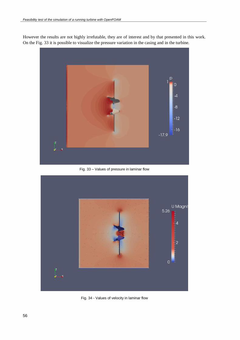
Feasibility test of the simulation of a running turbine with OpenFOAM
56
However the results are not highly irrefutable, they are of interest and by that presented in this work.
On the Fig. 33 it is possible to visualize the pressure variation in the casing and in the turbine.
Fig. 33 – Values of pressure in laminar flow
Fig. 34 - Values of velocity in laminar flow
Feasibility test of the simulation of a running turbine with OpenFOAM
57
The other feature that was studied was the velocity. In the Fig. 34 it is possible to verify the variations
in velocity. The results would be much more accurate it this studied was accomplished with turbulent
features.
Considering that the study of the flow while the turbine was running was not successfully
accomplished, it is not possible to compare numerical results of the values of velocity and pressure
near the turbine with the ones obtained so far by field and laboratory experiences.
Although the user-defined boundary conditions were already coded, it is possible to realize the
potential of an open-sourced software as OpenFOAM. It allows the user to modify the program with
new functionalities or even adapt the ones already created.
5.2. FUTURE WORKS
This work is only a small step in what can be done regarding hydraulic simulation and more precisely
the study of fish passage through hydroelectric turbines. The biggest advance that would improve
tremendously would be to solve the flow calculations while the mesh is in movement. The correlation
between velocity and pressure and how this affects concretely the fish would be necessary study. After
that, the next step could be the simulation of more detailed turbines and its casings.
Regarding the hydraulics conditions, the inlet and the outlet could be changed in order to approach the
numerical model to the reality for adding pipes or draft tubes.
Furthermore, it would be interesting to simulate cavitation in a three-dimensional mesh. It would be
interesting to study and control the interpolations between the deformed meshes and the new ones,
generated during the different time steps.
Studying a way of generating new meshes for different time steps instead of resorting to the
deformation of the same mesh, could lead to fewer errors while calculating the flows.

Feasibility test of the simulation of a running turbine with OpenFOAM
58
Feasibility testo f the simulation of a running turbine with OpenFOAM
59
BIBLIOGRAPHY:
Abernethy, Cary S., Brett G. Amidan, and G. F. Cada. (2001) "Laboratory studies of the effects of
pressure and dissolved gas supersaturation on turbine-passed fish." Pacific Northwest National
Laboratory, Richland, WA.
Anderson, J. D. (1995). “Computational fluid dynamics: The Basics with Applications” McGraw-
Hill. Inc., New York.
Bakker, A. (2002). Applied Computational Fluid Dynamics: Lecture 7- Meshing.
Bakker, A. (2002). Applied Computational Fluid Dynamics: Lecture 5 – Solution Methods.
Blazek, J. (2005). Computational Fluid Dynamics: Principles and Applications. Elsevier.
Čada, G.F. and Coutant, C.C. (1997). Development of Biological Criteria for the Design of Advanced
Hydropower Turbines.U.S. Department of Energy Idaho Operations Office, Idaho Falls, ID.
Čada, G. F. (2001). The development of advanced hydroelectric turbines to improve fish passage
survival. Fisheries, 26(9), 14-23.
Casadei, G. M. (2010). Dynamic-mesh techniques for unsteady multiphase surface-ship
hydrodynamics. The Pennsylvania State University.
Castro-Santos, T., Giza, D., Haro, A. J., Hecker, G., McMahon, B., Perkins, N., & Pioppi, N. (2012)
Environmental Effects of Hydrokinetic Turbines on Fish: Desktop and Laboratory Flume Studies.
Electric Power Research Institute.
Chen, W. L., Lien, F. S., & Leschziner, M. A. (1998). Non-linear eddy-viscosity modelling of
transitional boundary layers pertinent to turbomachine aerodynamics. International Journal of heat
and fluid flow, 19(4), 297-306.
Clifford, W.L. (1968). Diel Movement and vertical distribution of juvenile anadromous fish in turbine
intakes. Burreau of commercial fisheries fish-passage research program, Seattle, Wash.
Davies, J.K., (1988). A review of information relating to fish passage through turbines: implications to
tidal power schemes. Central Electricity Research Laboratories, Marine Biology Unit, Fawley,
Southampton, SO4 ITW, U.K.
Deng, Z., Carlson, T.J., Dauble, D.D. and Ploskey, G.R. (2011). Fish Passage Assessment of an
Advanced Hydropower Turbine and Conventional Turbine Using Blade-Strike Modeling. Pacific
Northwest National Laboratory, Richland, USA.
Dhakan, P. K., & Chalil, A. B. P. (2013). Design and construction of main casing for four jet vertical
pelton turbine. Engineering MECHANICS, 20(2), 77-88.
Eslamdoost, A., Nilsson, H., & Maus, K. J. (2009). Roll Motion of a Box and Interaction with Free-
Surface. Chalmers University of Technology.
Feathers, M. G., & Knable, A. E. (1983). Effects of depressurization upon largemouth bass. North
American Journal of Fisheries Management, 3(1), 86-90.
Ferguson, J.W. (2008). Behavior and Survival of Fish Migrating Downstream on Regulated Rivers.
Faculty of Forest Sciences, Department of Wildlife, Fish and Environmental Studies, Umea.
Feasibility testo f the simulation of a running turbine with OpenFOAM
60
Ferziger, J. H., & Peric, M. (2012). Computational methods for fluid dynamics. Springer Science &
Business Media.
Foye RE, Scott M. 1965. Effects of pressure on survival of six species of fish. Trans. Am. Fish.
Soc.94(1): 88-91
George, W. K. (2009). Lectures in Turbulence for the 21st Century. Chalmers University of
Technology.
González, A. O., Vallier, A., & Nilsson, H. (2009). Mesh motion alternatives in OpenFOAM. Götborg.
Sweden.
Harvey, Harold Henry. (1963) “Pressure in the early life history of sockeye salmon”. Diss. The
University of British Columbia.
Jacobson, P.T. (2012). Environmental Effects of Hydrokinetic Turbines on Fish: Desktop and
Laboratory Flume Studies. Electric Power Research Institute.
Jasak, H., & Rusche, H. (2009). Dynamic mesh handling in OpenFOAM. In Proceeding of the 47th
Aerospace Sciences Meeting Including the New Horizons Forum and Aerospace Exposition, Orlando,
FL.
Jones, W. P., & Menzies, K. R. (2000). Analysis of the cell-centred finite volume method for the
diffusion equation. Journal of Computational Physics,165(1), 45-68.
Kassiotis, C. (2008). Which strategy to move the mesh in the Computational Fluid Dynamic code
OpenFOAM. Report École Normale Supérieure de Cachan.
Killgore, K. J., Miller, A. C., & Conley, K. C. (1987). Effects of turbulence on yolk-sac larvae of
paddlefish. Transactions of the American Fisheries Society,116(4), 670-673.
Liu, Y., Pekkan, K., Jones, S. C., & Yoganathan, A. P. (2004). The effects of different mesh generation
methods on computational fluid dynamic analysis and power loss assessment in total cavopulmonary
connection. Journal of biomechanical engineering, 126(5), 594-603.
Markatos, N. C. (1986). The mathematical modelling of turbulent flows. Applied Mathematical
Modelling, 10(3), 190-220.
Mavriplis, D.J. (2002) Unstructured Mesh Related Issued In Computational Fluid Dynamics (CFD) –
Based Analysis and Design. NASA Langley Research Center. Hampton, VA 23681. USA.
Mazumdar, D., & Guthrie, R. I. L. (1995). On the numerical computation of turbulent fluid flow in
CAS steelmaking operations. Applied mathematical modelling, 19(9), 519-524.
McDonough, J. M. (2004). Introductory lectures on turbulence physics, mathematics and modeling.
Departments of Mechanical Engineering and Mathematics. University of Kentucky.
McEwen, D., & Scobie, G. (1992). Estimation of the hydraulic conditions relating to fish passage
through turbines. NPC001. National Engineering Laboratory, East Kilbride, Glasgow.
Munson, B. R., Young, D. F., & Okiishi, T. H. (1990). Fundamentals of fluid mechanics. New York.
Nichols, R. H. (2010). Turbulence models and their application to complex flows. University of
Alabama at Birmingham, Revision, 4, 89.
Feasibility testo f the simulation of a running turbine with OpenFOAM
61
Nilsson, H., Page, M., Beaudoin, M., Gschaider, B., & Jasak, H. (2008). The OpenFOAM
Turbomachinery working-group, and conclusions from the Turbomachinery session of the third
OpenFOAM workshop. In IAHR: 24th Symposium on Hydraulic Machinery and Systems, Foz do
Iguassu, Brazil.
OPENCFD, L. (2013). OpenFOAM: The Open Source CFD Toolbox.
Page, M., & Beaudoin, M. (2007). Adapting OpenFOAM for turbomachinery applications. In 2nd
OpenFOAM Workshop Zagreb, Croatia.
Rannacher, R. (2000). Finite element methods for the incompressible Navier-Stokes equations (pp.
191-293). Birkhäuser Basel.
Roger Ull, A. (2012). Study of mesh deformation features of an open source CFD package and
application to a gear pump simulation. Universitat Politècnica de Catalunya.
Rygg, J. R. (2013). CFD Analysis of a Pelton Turbine in OpenFOAM. Norwegian University of
Science and Technology.
Shewchuk, J. R. (1997). Delaunay refinement mesh generation. School of Computer Science.
Computer Science Department. Carnegie Mellon University. Pittsburgh, PA 15213.
Solomon, D. J. (1988). Fish passage through tidal energy barrages. Energy Technology Support Unit
(ETSU).
Sullivan, C.W. (1992). Fish Entrainment and Turbine Mortality Review and Guidelines. Research
Project 2694-01. Boston, Massachuetts.
Tennekes, H., & Lumley, J. L. (1972). A first course in turbulence. MIT press.
Therrien, J. and Bourgeois,G. (2000). Fish Passage at Small Hydro Sites. Report by Genivar
Consulting Group for CANMET Energy Technology Centre, Ottawa.
Turbak, S., Reichle, D.R. and Shriner, C.R. (1981). Analysis of environmental issues related to small-
scale hydroelectric development IV: Fish Mortality Resulting From Turbine Passage. Environmental
sciences division, publication No. 1597.
Turnpenny, A. W., Davis, M. H., Fleming, J. M., & Davies, J. K. (1992). Experimental Studies
Relating to the Passage of Fish and Shrimps Through Tidal Power Turbines. Marine and Freshwater
Biology Unit, National Power, Fawley, Southampton, Hampshire, England.
Uhlmann, M. (2012). Turbulenzmodelle in der Strömungsmechanik: RANS und LES. Institut für
Hydromechanik Karlsruher Institut für Technologie.
Versteeg, H. K., & Malalasekera, W. (1995). An introduction to computational fluid dynamics–The
finite volume method.
Versteeg, H. K., & Malalasekera, W. (2007). An introduction to computational fluid dynamics: the
finite volume method. Pearson Education.
Von Raben, K. (1957). Regarding the problem of mutilations of fishes by hydraulic turbines. Die
Wasserwirtschaft, 4, 97-100.
Watson, M. (1995). Allowable gas supersaturation for fish passing hydroelectric dams. Task 8. Bubble
reabsorption in a simulated smolt bypass system-concept assessment. U.S. Department of Energy
Bonneville Power Administration Environment, Fish and Wildlife P.O. Box 3621 Portland. OR
97208-3621.

Feasibility testo f the simulation of a running turbine with OpenFOAM
62
Wendt, J. E. (2008). Computational fluid dynamics: an introduction. Springer Science & Business
Media.
Williams, U.P., Scruton, D.A., Goosney, R.F., Bourgeois, C.E., Orr, D.C. and Ruggles, C.P. (1993).
Proceedings of the Workshop on Fish Passage at Hydroelectric Developments. St. John’s,
Newfoundland.
Yoganathan, A. P., He, Z., & Casey Jones, S. (2004). Fluid mechanics of heart valves. Annu. Rev.
Biomed. Eng., 6, 331-362.
Websites:
[1] http://www.daviddarling.info/encyclopedia/R/AE_reaction_turbine.html. April, 2015.
[2] http://www.learnengineering.org/2013/08/kaplan-turbine-hodroelectric-power-gneration.html.
April, 2015
[3] http://www.learnengineering.org/2014/01/how-does-francis-turbine-work.html. April, 2015
[4] http://www.fao.org/docrep/004/y2785e/y2785e03.htm. Março 2015. March, 2015.
[5] http://www.ebah.pt/content/ABAAAATzIAE/tipos-turbinas-hidraulicas?part=2. May 2015
[6] http://www.bakker.org/. May 2015
[7] http://www.cfd-online.com/Wiki/Mesh_classification. May 2015
[8] http://www.pointwise.com/theconnector/March-2013/Structured-Grids-in-Pointwise.shtml. April
2015
[9] http://www.mathematik.uni-dortmund.de/~kuzmin/cfdintro/lecture1.pdf. April 2015
[10] http://noc.ac.uk/f/content/science-technology/workshops/presentation_2_meshing.pdf. April,
2015.
[11] http://www.renewablesfirst.co.uk/hydro-learning-centre/kaplan-turbines/ March, 2015.

63
Appendix
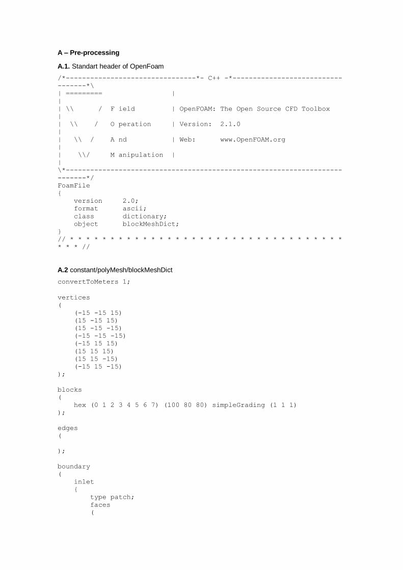
A – Pre-processing
A.1. Standart header of OpenFoam
/*--------------------------------*- C++ -*---------------------------
-------*\
| ========= |
|
| \\ / F ield | OpenFOAM: The Open Source CFD Toolbox
|
| \\ / O peration | Version: 2.1.0
|
| \\ / A nd | Web: www.OpenFOAM.org
|
| \\/ M anipulation |
|
\*--------------------------------------------------------------------
-------*/
FoamFile
{
version 2.0;
format ascii;
class dictionary;
object blockMeshDict;
}
// * * * * * * * * * * * * * * * * * * * * * * * * * * * * * * * * * *
* * * //
A.2 constant/polyMesh/blockMeshDict
convertToMeters 1;
vertices
(
(-15 -15 15)
(15 -15 15)
(15 -15 -15)
(-15 -15 -15)
(-15 15 15)
(15 15 15)
(15 15 -15)
(-15 15 -15)
);
blocks
(
hex (0 1 2 3 4 5 6 7) (100 80 80) simpleGrading (1 1 1)
);
edges
(
);
boundary
(
inlet
{
type patch;
faces
(
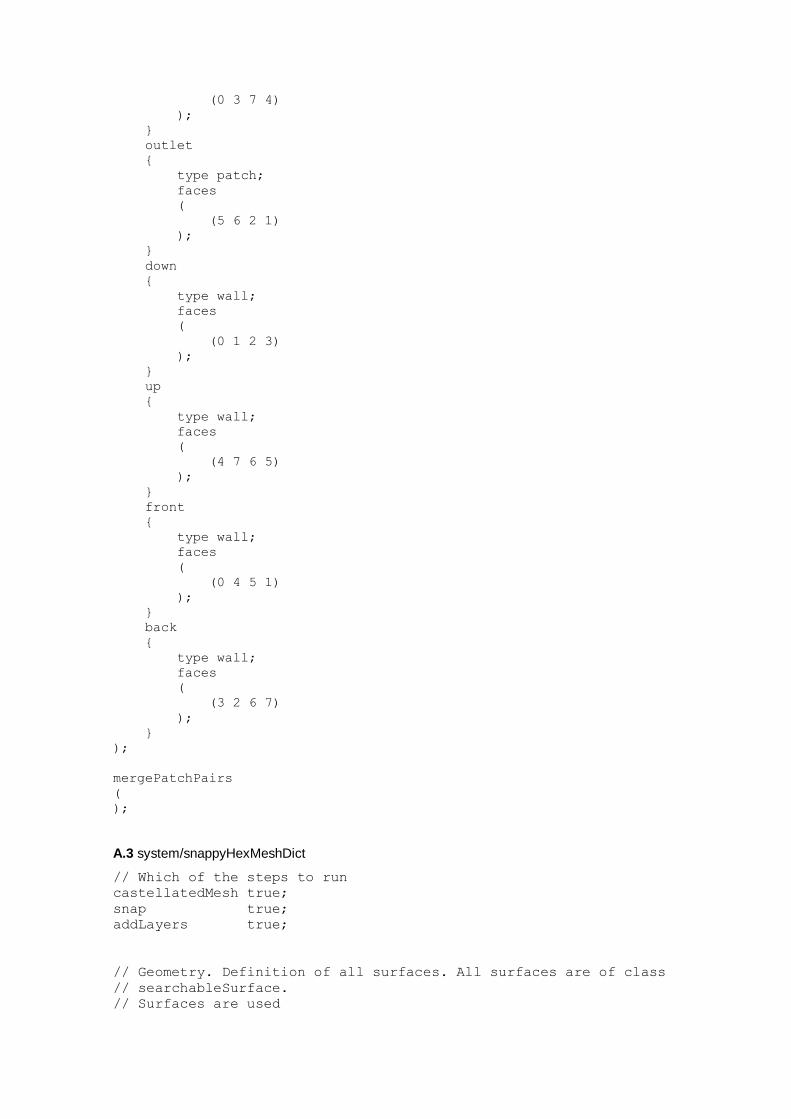
(0 3 7 4)
);
}
outlet
{
type patch;
faces
(
(5 6 2 1)
);
}
down
{
type wall;
faces
(
(0 1 2 3)
);
}
up
{
type wall;
faces
(
(4 7 6 5)
);
}
front
{
type wall;
faces
(
(0 4 5 1)
);
}
back
{
type wall;
faces
(
(3 2 6 7)
);
}
);
mergePatchPairs
(
);
A.3 system/snappyHexMeshDict
// Which of the steps to run
castellatedMesh true;
snap true;
addLayers true;
// Geometry. Definition of all surfaces. All surfaces are of class
// searchableSurface.
// Surfaces are used
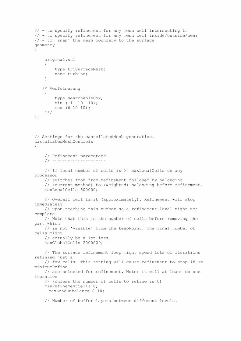
// - to specify refinement for any mesh cell intersecting it
// - to specify refinement for any mesh cell inside/outside/near
// - to 'snap' the mesh boundary to the surface
geometry
{
original.stl
{
type triSurfaceMesh;
name turbine;
}
/* Verfeinerung
{
type searchableBox;
min (-1 -10 -10);
max (6 10 10);
}*/
};
// Settings for the castellatedMesh generation.
castellatedMeshControls
{
// Refinement parameters
// ~~~~~~~~~~~~~~~~~~~~~
// If local number of cells is >= maxLocalCells on any
processor
// switches from from refinement followed by balancing
// (current method) to (weighted) balancing before refinement.
maxLocalCells 500000;
// Overall cell limit (approximately). Refinement will stop
immediately
// upon reaching this number so a refinement level might not
complete.
// Note that this is the number of cells before removing the
part which
// is not 'visible' from the keepPoint. The final number of
cells might
// actually be a lot less.
maxGlobalCells 2000000;
// The surface refinement loop might spend lots of iterations
refining just a
// few cells. This setting will cause refinement to stop if <=
minimumRefine
// are selected for refinement. Note: it will at least do one
iteration
// (unless the number of cells to refine is 0)
minRefinementCells 0;
maxLoadUnbalance 0.10;
// Number of buffer layers between different levels.
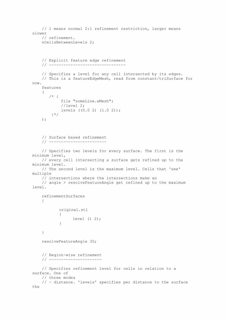
// 1 means normal 2:1 refinement restriction, larger means
slower
// refinement.
nCellsBetweenLevels 2;
// Explicit feature edge refinement
// ~~~~~~~~~~~~~~~~~~~~~~~~~~~~~~~~
// Specifies a level for any cell intersected by its edges.
// This is a featureEdgeMesh, read from constant/triSurface for
now.
features
(
/* {
file "someLine.eMesh";
//level 2;
levels ((0.0 2) (1.0 2));
}*/
);
// Surface based refinement
// ~~~~~~~~~~~~~~~~~~~~~~~~
// Specifies two levels for every surface. The first is the
minimum level,
// every cell intersecting a surface gets refined up to the
minimum level.
// The second level is the maximum level. Cells that 'see'
multiple
// intersections where the intersections make an
// angle > resolveFeatureAngle get refined up to the maximum
level.
refinementSurfaces
{
original.stl
{
level (1 2);
}
}
resolveFeatureAngle 30;
// Region-wise refinement
// ~~~~~~~~~~~~~~~~~~~~~~
// Specifies refinement level for cells in relation to a
surface. One of
// three modes
// - distance. 'levels' specifies per distance to the surface
the
// wanted refinement level. The distances need to be
specified in
// descending order.
// - inside. 'levels' is only one entry and only the level is
used. All
// cells inside the surface get refined up to the level. The
surface
// needs to be closed for this to be possible.
// - outside. Same but cells outside.
refinementRegions
{
/*Verfeinerung
{
mode inside;
levels ((1 4));
}*/
}
// Mesh selection
// ~~~~~~~~~~~~~~
// After refinement patches get added for all
refinementSurfaces and
// all cells intersecting the surfaces get put into these
patches. The
// section reachable from the locationInMesh is kept.
// NOTE: This point should never be on a face, always inside a
cell, even
// after refinement.
// This is an outside point locationInMesh (-0.033 -0.033
0.0033);
locationInMesh (-10 -10 10); // Inside point
// Whether any faceZones (as specified in the
refinementSurfaces)
// are only on the boundary of corresponding cellZones or also
allow
// free-standing zone faces. Not used if there are no
faceZones.
allowFreeStandingZoneFaces true;
}
// Settings for the snapping.
snapControls
{
//- Number of patch smoothing iterations before finding
correspondence
// to surface
nSmoothPatch 10;
//- Relative distance for points to be attracted by surface
feature point
// or edge. True distance is this factor times local
// maximum edge length.
tolerance 1.2;
//- Number of mesh displacement relaxation iterations.
nSolveIter 10;
//- Maximum number of snapping relaxation iterations. Should
stop
// before upon reaching a correct mesh.
nRelaxIter 3;
//- Highly experimental and wip: number of feature edge
snapping
// iterations. Leave out altogether to disable.
nFeatureSnapIter 10;
}
// Settings for the layer addition.
addLayersControls
{
// Are the thickness parameters below relative to the
undistorted
// size of the refined cell outside layer (true) or absolute
sizes (false).
relativeSizes true;
// Per final patch (so not geometry!) the layer information
layers
{
"turbine.*"
{
nSurfaceLayers 5;
}
}
// Expansion factor for layer mesh
expansionRatio 1.5;
//- Wanted thickness of final added cell layer. If multiple
layers
// is the thickness of the layer furthest away from the wall.
// See relativeSizes parameter.
finalLayerThickness 0.8;
//- Minimum thickness of cell layer. If for any reason layer
// cannot be above minThickness do not add layer.
// See relativeSizes parameter.
minThickness 0.001;
//- If points get not extruded do nGrow layers of connected
faces that are
// also not grown. This helps convergence of the layer
addition process
// close to features.
nGrow 0;
// Advanced settings
//- When not to extrude surface. 0 is flat surface, 90 is when
two faces
// make straight angle.
featureAngle 30;
//- Maximum number of snapping relaxation iterations. Should
stop
// before upon reaching a correct mesh.
nRelaxIter 5;
// Number of smoothing iterations of surface normals
nSmoothSurfaceNormals 1;
// Number of smoothing iterations of interior mesh movement
direction
nSmoothNormals 3;
// Smooth layer thickness over surface patches
nSmoothThickness 10;
// Stop layer growth on highly warped cells
maxFaceThicknessRatio 0.5;
// Reduce layer growth where ratio thickness to medial
// distance is large
maxThicknessToMedialRatio 0.4;
// Angle used to pick up medial axis points
minMedianAxisAngle 130;
// Create buffer region for new layer terminations
nBufferCellsNoExtrude 0;
// Overall max number of layer addition iterations. The mesher
will exit
// if it reaches this number of iterations; possibly with an
illegal
// mesh.
nLayerIter 50;
// Max number of iterations after which relaxed meshQuality
controls
// get used. Up to nRelaxIter it uses the settings in
meshQualityControls,
// after nRelaxIter it uses the values in
meshQualityControls::relaxed.
nRelaxedIter 20;
}
// Generic mesh quality settings. At any undoable phase these
determine
// where to undo.
meshQualityControls
{
//- Maximum non-orthogonality allowed. Set to 180 to disable.
maxNonOrtho 60;
//- Max skewness allowed. Set to <0 to disable.
maxBoundarySkewness 20;
maxInternalSkewness 4;
//- Max concaveness allowed. Is angle (in degrees) below which
concavity
// is allowed. 0 is straight face, <0 would be convex face.
// Set to 180 to disable.
maxConcave 80;
//- Minimum pyramid volume. Is absolute volume of cell pyramid.
// Set to a sensible fraction of the smallest cell volume
expected.
// Set to very negative number (e.g. -1E30) to disable.
minVol 1e-13;
//- Minimum quality of the tet formed by the face-centre
// and variable base point minimum decomposition triangles and
// the cell centre. Set to very negative number (e.g. -1E30)
to
// disable.
// <0 = inside out tet,
// 0 = flat tet
// 1 = regular tet
minTetQuality 1e-30;
//- Minimum face area. Set to <0 to disable.
minArea -1;
//- Minimum face twist. Set to <-1 to disable. dot product of
face normal
//- and face centre triangles normal
minTwist 0.05;
//- minimum normalised cell determinant
//- 1 = hex, <= 0 = folded or flattened illegal cell
minDeterminant 0.001;
//- minFaceWeight (0 -> 0.5)
minFaceWeight 0.05;
//- minVolRatio (0 -> 1)
minVolRatio 0.01;
//must be >0 for Fluent compatibility
minTriangleTwist -1;
//- if >0 : preserve single cells with all points on the
surface if the
// resulting volume after snapping (by approximation) is
larger than
// minVolCollapseRatio times old volume (i.e. not collapsed to
flat cell).
// If <0 : delete always.
//minVolCollapseRatio 0.5;
// Advanced
//- Number of error distribution iterations
nSmoothScale 4;
//- amount to scale back displacement at error points
errorReduction 0.75;
// Optional : some meshing phases allow usage of relaxed rules.
// See e.g. addLayersControls::nRelaxedIter.
relaxed
{
//- Maximum non-orthogonality allowed. Set to 180 to
disable.
maxNonOrtho 75;
}
}
// Advanced
// Flags for optional output
// 0 : only write final meshes
// 1 : write intermediate meshes
// 2 : write volScalarField with cellLevel for postprocessing
// 4 : write current intersections as .obj files
debug 0;
// Merge tolerance. Is fraction of overall bounding box of initial
mesh.
// Note: the write tolerance needs to be higher than this.
mergeTolerance 1E-6;
A.4 0/p
dimensions [0 2 -2 0 0 0 0];
internalField uniform 0;
boundaryField
{
inlet //inlet
{
type zeroGradient;
}
outlet //outlet
{
type fixedValue;
value uniform 0;
}
left //wall
{
type zeroGradient;
}
right //wall
{
type zeroGradient;
}
down //wall
{
type zeroGradient;
}
up //wall
{
type zeroGradient;
}
front //wall
{
type zeroGradient;
}
back //wall
{
type zeroGradient;
}
turbine_patch28539 //wall
{
type zeroGradient;
}
atmosphere
{
type zeroGradient;
}
defaultFaces
{
type empty;
}
procBoundary0to1
{
type processor;
}
procBoundary0to2
{
type processor;
}
procBoundary0to3
{
type processor;
}
procBoundary0to4
{
type processor;
}
procBoundary0to5
{
type processor;
}
procBoundary1to0
{
type processor;
}
procBoundary1to2
{
type processor;
}
procBoundary1to3
{
type processor;
}
procBoundary1to4
{
type processor;
}
procBoundary1to5
{
type processor;
}
procBoundary2to0
{
type processor;
}
procBoundary2to1
{
type processor;
}
procBoundary2to3
{
type processor;
}
procBoundary2to6
{
type processor;
}
procBoundary2to7
{
type processor;
}

procBoundary3to0
{
type processor;
}
procBoundary3to1
{
type processor;
}
procBoundary3to2
{
type processor;
}
procBoundary3to6
{
type processor;
}
procBoundary3to7
{
type processor;
}
procBoundary4to0
{
type processor;
}
procBoundary4to1
{
type processor;
}
procBoundary4to5
{
type processor;
}
procBoundary4to6
{
type processor;
}
procBoundary4to7
{
type processor;
}
procBoundary5to0
{
type processor;
}
procBoundary5to1
{
type processor;
}
procBoundary5to4
{
type processor;
}
procBoundary5to6
{
type processor;
}
procBoundary5to7
{
type processor;
}
procBoundary6to2
{
type processor;
}
procBoundary6to3
{
type processor;
}
procBoundary6to4
{
type processor;
}
procBoundary6to5
{
type processor;
}
procBoundary6to7
{
type processor;
}
procBoundary7to2
{
type processor;
}
procBoundary7to3
{
type processor;
}
procBoundary7to4
{
type processor;
}
procBoundary7to5

{
type processor;
}
procBoundary7to6
{
type processor;
}
}
A.5 0/U
dimensions [0 1 -1 0 0 0 0];
internalField uniform (0 0 0);
boundaryField
{
inlet
{
type fixedValue;
value uniform (1 0 0);
}
outlet
{
type inletOutlet;
inletValue uniform (0 0 0);
value uniform (0 0 0);
}
down
{
type fixedValue;
value uniform (0 0 0);
}
up
{
type fixedValue;
value uniform (0 0 0);
}
front
{
type fixedValue;
value uniform (0 0 0);
}
back
{
type fixedValue;
value uniform (0 0 0);
}
turbine_patch28539
{
type fixedValue;
value uniform (0 0 0);
}
procBoundary0to1
{
type processor;
}
procBoundary0to2
{
type processor;
}
procBoundary0to3
{
type processor;
}
procBoundary0to4
{
type processor;
}
procBoundary0to5
{
type processor;
}
procBoundary1to0
{
type processor;
}
procBoundary1to2
{
type processor;
}
procBoundary1to3
{
type processor;
}
procBoundary1to4
{
type processor;
}
procBoundary1to5
{
type processor;
}
procBoundary2to0
{
type processor;
}
procBoundary2to1
{
type processor;
}
procBoundary2to3
{
type processor;
}
procBoundary2to6
{
type processor;
}
procBoundary2to7
{
type processor;
}
procBoundary3to0
{
type processor;
}
procBoundary3to1
{
type processor;
}
procBoundary3to2
{
type processor;
}
procBoundary3to6
{
type processor;
}
procBoundary3to7
{
type processor;
}
procBoundary4to0
{
type processor;
}
procBoundary4to1
{
type processor;
}
procBoundary4to5
{
type processor;
}
procBoundary4to6
{
type processor;
}
procBoundary4to7
{
type processor;
}
procBoundary5to0
{
type processor;
}
procBoundary5to1
{
type processor;
}
procBoundary5to4
{
type processor;
}
procBoundary5to6
{
type processor;
}
procBoundary5to7
{
type processor;
}
procBoundary6to2
{
type processor;
}
procBoundary6to3
{
type processor;
}
procBoundary6to4
{
type processor;
}
procBoundary6to5
{
type processor;
}
procBoundary6to7
{
type processor;
}
procBoundary7to2
{
type processor;
}
procBoundary7to3
{
type processor;
}
procBoundary7to4
{
type processor;
}
procBoundary7to5
{
type processor;
}
procBoundary7to6
{
type processor;
}
}
A.6 0/k
dimensions [ 0 2 -2 0 0 0 0 ];
internalField uniform 1;
boundaryField
{
inlet
{
type turbulentIntensityKineticEnergyInlet;
intensity 0.05; // 5% turbulent intensity
value uniform 1;
}
outlet
{
type inletOutlet;
inletValue uniform 1;
}
down
{
type kqRWallFunction;
value uniform 0;
}
up
{
type kqRWallFunction;
value uniform 0;
}
front
{
type kqRWallFunction;
value uniform 0;
}
back
{
type kqRWallFunction;
value uniform 0;
}
turbine_patch28539
{
type kqRWallFunction;
value uniform 0;
}
procBoundary0to1
{
type processor;
}
procBoundary0to2
{
type processor;
}
procBoundary0to3
{
type processor;
}
procBoundary0to4
{
type processor;
}
procBoundary0to5
{
type processor;
}
procBoundary1to0
{
type processor;
}
procBoundary1to2
{
type processor;
}
procBoundary1to3
{
type processor;
}
procBoundary1to4
{
type processor;
}
procBoundary1to5
{
type processor;
}
procBoundary2to0
{
type processor;
}
procBoundary2to1
{
type processor;
}
procBoundary2to3
{
type processor;
}
procBoundary2to6
{
type processor;
}
procBoundary2to7
{
type processor;
}
procBoundary3to0
{
type processor;
}
procBoundary3to1
{
type processor;
}
procBoundary3to2
{
type processor;
}
procBoundary3to6
{
type processor;
}
procBoundary3to7
{
type processor;
}
procBoundary4to0
{
type processor;
}
procBoundary4to1
{
type processor;
}
procBoundary4to5
{
type processor;
}
procBoundary4to6
{
type processor;
}
procBoundary4to7
{
type processor;
}
procBoundary5to0
{
type processor;
}
procBoundary5to1
{
type processor;
}
procBoundary5to4
{
type processor;
}
procBoundary5to6
{
type processor;
}
procBoundary5to7
{
type processor;
}
procBoundary6to2
{
type processor;
}
procBoundary6to3
{
type processor;
}
procBoundary6to4
{
type processor;
}
procBoundary6to5
{
type processor;
}
procBoundary6to7
{
type processor;
}
procBoundary7to2
{
type processor;
}
procBoundary7to3
{
type processor;
}
procBoundary7to4
{
type processor;
}
procBoundary7to5
{
type processor;
}
procBoundary7to6
{
type processor;
}
}
A.7 0/omega
dimensions [0 0 -1 0 0 0 0];
internalField uniform 0.001;
boundaryField
{
inlet
{
type turbulentMixingLengthFrequencyInlet;
mixingLength 0.01; // 1cm - half channel height
k k;
value uniform 1;
}
outlet
{
type inletOutlet;
inletValue uniform 1;
}
down
{
type omegaWallFunction;
value uniform 0;
}
up
{
type omegaWallFunction;
value uniform 0;
}
front
{
type omegaWallFunction;
value uniform 0;
}
back
{
type omegaWallFunction;
value uniform 0;
}
turbine_patch28539
{
type omegaWallFunction;
value uniform 0;
}
procBoundary0to1
{
type processor;
}
procBoundary0to2
{
type processor;
}
procBoundary0to3
{
type processor;
}
procBoundary0to4
{

type processor;
}
procBoundary0to5
{
type processor;
}
procBoundary1to0
{
type processor;
}
procBoundary1to2
{
type processor;
}
procBoundary1to3
{
type processor;
}
procBoundary1to4
{
type processor;
}
procBoundary1to5
{
type processor;
}
procBoundary2to0
{
type processor;
}
procBoundary2to1
{
type processor;
}
procBoundary2to3
{
type processor;
}
procBoundary2to6
{
type processor;
}
procBoundary2to7
{
type processor;
}
procBoundary3to0
{
type processor;
}
procBoundary3to1
{
type processor;
}
procBoundary3to2
{
type processor;
}
procBoundary3to6
{
type processor;
}
procBoundary3to7
{
type processor;
}
procBoundary4to0
{
type processor;
}
procBoundary4to1
{
type processor;
}
procBoundary4to5
{
type processor;
}
procBoundary4to6
{
type processor;
}
procBoundary4to7
{
type processor;
}
procBoundary5to0
{
type processor;
}
procBoundary5to1
{
type processor;

}
procBoundary5to4
{
type processor;
}
procBoundary5to6
{
type processor;
}
procBoundary5to7
{
type processor;
}
procBoundary6to2
{
type processor;
}
procBoundary6to3
{
type processor;
}
procBoundary6to4
{
type processor;
}
procBoundary6to5
{
type processor;
}
procBoundary6to7
{
type processor;
}
procBoundary7to2
{
type processor;
}
procBoundary7to3
{
type processor;
}
procBoundary7to4
{
type processor;
}
procBoundary7to5

{
type processor;
}
procBoundary7to6
{
type processor;
}
}
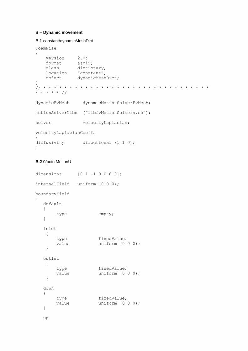
B – Dynamic movement
B.1 constant/dynamicMeshDict
FoamFile
{
version 2.0;
format ascii;
class dictionary;
location "constant";
object dynamicMeshDict;
}
// * * * * * * * * * * * * * * * * * * * * * * * * * * * * * * * *
* * * * * //
dynamicFvMesh dynamicMotionSolverFvMesh;
motionSolverLibs ("libfvMotionSolvers.so");
solver velocityLaplacian;
velocityLaplacianCoeffs
{
diffusivity directional (1 1 0);
}
B.2 0/pointMotionU
dimensions [0 1 -1 0 0 0 0];
internalField uniform (0 0 0);
boundaryField
{
default
{
type empty;
}
inlet
{
type fixedValue;
value uniform (0 0 0);
}
outlet
{
type fixedValue;
value uniform (0 0 0);
}
down
{
type fixedValue;
value uniform (0 0 0);
}
up
{
type fixedValue;
value uniform (0 0 0);
}
front
{
type fixedValue;
value uniform (0 0 0);
}
back
{
type fixedValue;
value uniform (0 0 0);
}
turbine_patch28539
{
type libAngularVelocity;
axis (1 0 0);
origin (0 0 0);
angle0 0;
omega 20.94; //200 rpm
value uniform (1 0 0);
}
procBoundary0to1
{
type processor;
}
procBoundary0to2
{
type processor;
}
procBoundary0to3
{
type processor;
}
procBoundary0to4
{
type processor;
}
procBoundary0to5
{
type processor;
}
procBoundary1to0
{
type processor;
}
procBoundary1to2
{
type processor;
}
procBoundary1to3
{
type processor;
}
procBoundary1to4
{
type processor;
}
procBoundary1to5
{
type processor;
}
procBoundary2to0
{
type processor;
}
procBoundary2to1
{
type processor;
}
procBoundary2to3
{
type processor;
}
procBoundary2to6
{
type processor;
}
procBoundary2to7
{
type processor;
}
procBoundary3to0
{
type processor;
}
procBoundary3to1
{
type processor;
}
procBoundary3to2
{
type processor;
}
procBoundary3to6
{
type processor;
}
procBoundary3to7
{
type processor;
}
procBoundary4to0
{
type processor;
}
procBoundary4to1
{
type processor;
}
procBoundary4to5
{
type processor;
}
procBoundary4to6
{
type processor;
}
procBoundary4to7
{
type processor;
}
procBoundary5to0
{
type processor;
}
procBoundary5to1
{
type processor;
}
procBoundary5to4
{
type processor;
}
procBoundary5to7
{
type processor;
}
procBoundary5to6
{
type processor;
}
procBoundary6to2
{
type processor;
}
procBoundary6to3
{
type processor;
}
procBoundary6to4
{
type processor;
}
procBoundary6to5
{
type processor;
}
procBoundary6to7
{
type processor;
}
procBoundary7to2
{
type processor;
}
procBoundary7to3
{
type processor;
}
procBoundary7to4
{
type processor;
}
procBoundary7to5
{
type processor;
}
procBoundary7to6
{
type processor;
}
}
B.3 0/cellMotionU
dimensions [0 1 -1 0 0 0 0];
internalField uniform (0 0 0);
boundaryField
{
default
{
type empty;
}
inlet
{
type fixedValue;
value uniform (0 0 0);
}
outlet
{
type fixedValue;
value uniform (0 0 0);
}
down
{
type fixedValue;
value uniform (0 0 0);
}
up
{
type fixedValue;
value uniform (0 0 0);
}
front
{
type fixedValue;
value uniform (0 0 0);
}
back
{
type fixedValue;
value uniform (0 0 0);
}
turbine_patch28539
{
type rotatingWallVelocity;
axis (1 0 0);
origin (0 0 0);
angle0 0;
omega 20.94
value uniform (1 0 0);
}
procBoundary0to1
{
type processor;
}
procBoundary0to2
{
type processor;
}
procBoundary0to3
{
type processor;
}
procBoundary0to4
{
type processor;
}
procBoundary0to5
{
type processor;
}
procBoundary1to0
{
type processor;
}
procBoundary1to2
{
type processor;
}
procBoundary1to3
{
type processor;
}
procBoundary1to4
{
type processor;
}
procBoundary1to5
{
type processor;
}
procBoundary2to0
{
type processor;
}
procBoundary2to1
{
type processor;
}
procBoundary2to3
{
type processor;
}
procBoundary2to6
{
type processor;
}
procBoundary2to7
{
type processor;
}
procBoundary3to0
{
type processor;
}
procBoundary3to1
{
type processor;
}
procBoundary3to2
{
type processor;
}
procBoundary3to6
{
type processor;
}
procBoundary3to7
{
type processor;
}
procBoundary4to0
{
type processor;
}
procBoundary4to1
{
type processor;
}
procBoundary4to5
{
type processor;
}
procBoundary4to6
{
type processor;
}
procBoundary4to7
{
type processor;
}
procBoundary5to0
{
type processor;
}
procBoundary5to1
{
type processor;
}
procBoundary5to4
{
type processor;
}
procBoundary5to7
{
type processor;
}
procBoundary6to2
{
type processor;
}
procBoundary6to3
{
type processor;
}
procBoundary6to4
{
type processor;
}
procBoundary6to7
{
type processor;
}
procBoundary7to2
{
type processor;
}
procBoundary7to3
{
type processor;
}
procBoundary7to4
{
type processor;
}
procBoundary7to5
{
type processor;
}
procBoundary7to6
{
type processor;
C – Solving
C.1 constant/turbulenceProperties
FoamFile
{
version 2.0;
format ascii;
class dictionary;
location "constant";
object turbulenceProperties;
}
// * * * * * * * * * * * * * * * * * * * * * * * * * * * * * * * *
* * * * * //
simulationType RASModel;
C.2 constant/RASProperties
FoamFile
{
version 2.0;
format ascii;
class dictionary;
location "constant";
object RASProperties;
}
// * * * * * * * * * * * * * * * * * * * * * * * * * * * * * * * *
* * * * * //
RASModel kOmegaSST;
turbulence on;
printCoeffs on;
C.3 constant/transportProperties
FoamFile
{
version 2.0;
format ascii;
class dictionary;
location "constant";
object transportProperties;
}
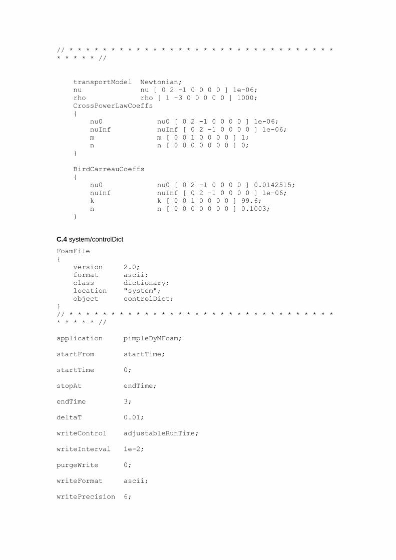
// * * * * * * * * * * * * * * * * * * * * * * * * * * * * * * * *
* * * * * //
transportModel Newtonian;
nu nu [ 0 2 -1 0 0 0 0 ] 1e-06;
rho rho [ 1 -3 0 0 0 0 0 ] 1000;
CrossPowerLawCoeffs
{
nu0 nu0 [ 0 2 -1 0 0 0 0 ] 1e-06;
nuInf nuInf [ 0 2 -1 0 0 0 0 ] 1e-06;
m m [ 0 0 1 0 0 0 0 ] 1;
n n [ 0 0 0 0 0 0 0 ] 0;
}
BirdCarreauCoeffs
{
nu0 nu0 [ 0 2 -1 0 0 0 0 ] 0.0142515;
nuInf nuInf [ 0 2 -1 0 0 0 0 ] 1e-06;
k k [ 0 0 1 0 0 0 0 ] 99.6;
n n [ 0 0 0 0 0 0 0 ] 0.1003;
}
C.4 system/controlDict
FoamFile
{
version 2.0;
format ascii;
class dictionary;
location "system";
object controlDict;
}
// * * * * * * * * * * * * * * * * * * * * * * * * * * * * * * * *
* * * * * //
application pimpleDyMFoam;
startFrom startTime;
startTime 0;
stopAt endTime;
endTime 3;
deltaT 0.01;
writeControl adjustableRunTime;
writeInterval 1e-2;
purgeWrite 0;
writeFormat ascii;
writePrecision 6;
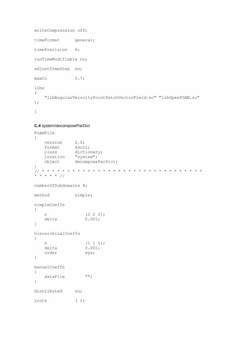
writeCompression off;
timeFormat general;
timePrecision 6;
runTimeModifiable no;
adjustTimeStep no;
maxCo 0.7;
libs
(
"libAngularVelocityPointPatchVectorField.so" "libOpenFOAM.so"
);
}
C.4 system/decomposeParDict
FoamFile
{
version 2.0;
format ascii;
class dictionary;
location "system";
object decomposeParDict;
}
// * * * * * * * * * * * * * * * * * * * * * * * * * * * * * * * *
* * * * * //
numberOfSubdomains 8;
method simple;
simpleCoeffs
{
n (2 2 2);
delta 0.001;
}
hierarchicalCoeffs
{
n (1 1 1);
delta 0.001;
order xyz;
}
manualCoeffs
{
dataFile "";
}
distributed no;
roots ( );
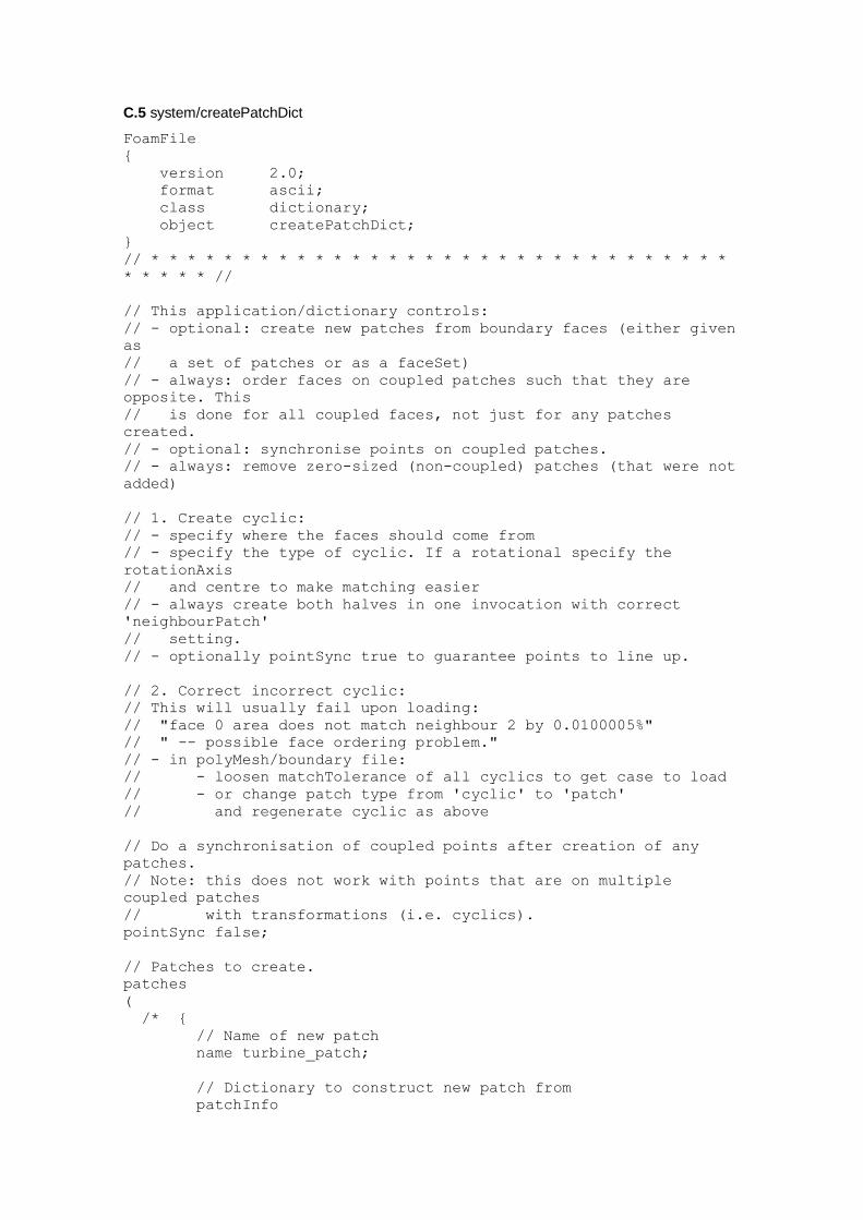
C.5 system/createPatchDict
FoamFile
{
version 2.0;
format ascii;
class dictionary;
object createPatchDict;
}
// * * * * * * * * * * * * * * * * * * * * * * * * * * * * * * * *
* * * * * //
// This application/dictionary controls:
// - optional: create new patches from boundary faces (either given
as
// a set of patches or as a faceSet)
// - always: order faces on coupled patches such that they are
opposite. This
// is done for all coupled faces, not just for any patches
created.
// - optional: synchronise points on coupled patches.
// - always: remove zero-sized (non-coupled) patches (that were not
added)
// 1. Create cyclic:
// - specify where the faces should come from
// - specify the type of cyclic. If a rotational specify the
rotationAxis
// and centre to make matching easier
// - always create both halves in one invocation with correct
'neighbourPatch'
// setting.
// - optionally pointSync true to guarantee points to line up.
// 2. Correct incorrect cyclic:
// This will usually fail upon loading:
// "face 0 area does not match neighbour 2 by 0.0100005%"
// " -- possible face ordering problem."
// - in polyMesh/boundary file:
// - loosen matchTolerance of all cyclics to get case to load
// - or change patch type from 'cyclic' to 'patch'
// and regenerate cyclic as above
// Do a synchronisation of coupled points after creation of any
patches.
// Note: this does not work with points that are on multiple
coupled patches
// with transformations (i.e. cyclics).
pointSync false;
// Patches to create.
patches
(
/* {
// Name of new patch
name turbine_patch;
// Dictionary to construct new patch from
patchInfo
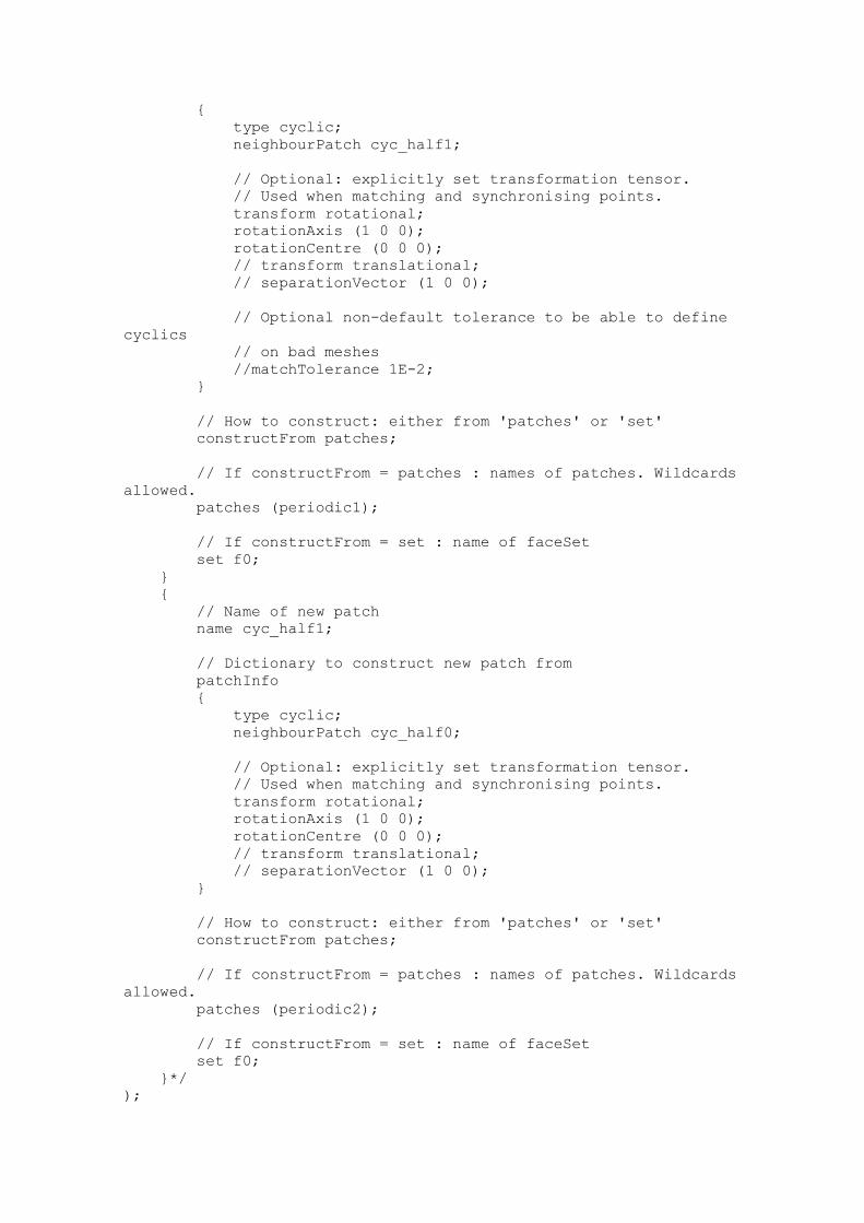
{
type cyclic;
neighbourPatch cyc_half1;
// Optional: explicitly set transformation tensor.
// Used when matching and synchronising points.
transform rotational;
rotationAxis (1 0 0);
rotationCentre (0 0 0);
// transform translational;
// separationVector (1 0 0);
// Optional non-default tolerance to be able to define
cyclics
// on bad meshes
//matchTolerance 1E-2;
}
// How to construct: either from 'patches' or 'set'
constructFrom patches;
// If constructFrom = patches : names of patches. Wildcards
allowed.
patches (periodic1);
// If constructFrom = set : name of faceSet
set f0;
}
{
// Name of new patch
name cyc_half1;
// Dictionary to construct new patch from
patchInfo
{
type cyclic;
neighbourPatch cyc_half0;
// Optional: explicitly set transformation tensor.
// Used when matching and synchronising points.
transform rotational;
rotationAxis (1 0 0);
rotationCentre (0 0 0);
// transform translational;
// separationVector (1 0 0);
}
// How to construct: either from 'patches' or 'set'
constructFrom patches;
// If constructFrom = patches : names of patches. Wildcards
allowed.
patches (periodic2);
// If constructFrom = set : name of faceSet
set f0;
}*/
);
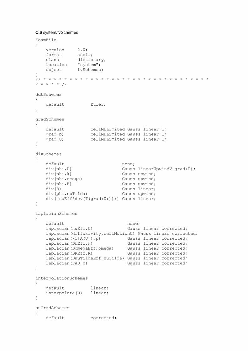
C.6 system/fvSchemes
FoamFile
{
version 2.0;
format ascii;
class dictionary;
location "system";
object fvSchemes;
}
// * * * * * * * * * * * * * * * * * * * * * * * * * * * * * * * *
* * * * * //
ddtSchemes
{
default Euler;
}
gradSchemes
{
default cellMDLimited Gauss linear 1;
grad(p) cellMDLimited Gauss linear 1;
grad(U) cellMDLimited Gauss linear 1;
}
divSchemes
{
default none;
div(phi,U) Gauss linearUpwindV grad(U);
div(phi,k) Gauss upwind;
div(phi,omega) Gauss upwind;
div(phi,R) Gauss upwind;
div(R) Gauss linear;
div(phi,nuTilda) Gauss upwind;
div((nuEff*dev(T(grad(U))))) Gauss linear;
}
laplacianSchemes
{
default none;
laplacian(nuEff,U) Gauss linear corrected;
laplacian(diffusivity,cellMotionU) Gauss linear corrected;
laplacian((1|A(U)),p) Gauss linear corrected;
laplacian(DkEff,k) Gauss linear corrected;
laplacian(DomegaEff,omega) Gauss linear corrected;
laplacian(DREff,R) Gauss linear corrected;
laplacian(DnuTildaEff,nuTilda) Gauss linear corrected;
laplacian(rAU,p) Gauss linear corrected;
}
interpolationSchemes
{
default linear;
interpolate(U) linear;
}
snGradSchemes
{
default corrected;
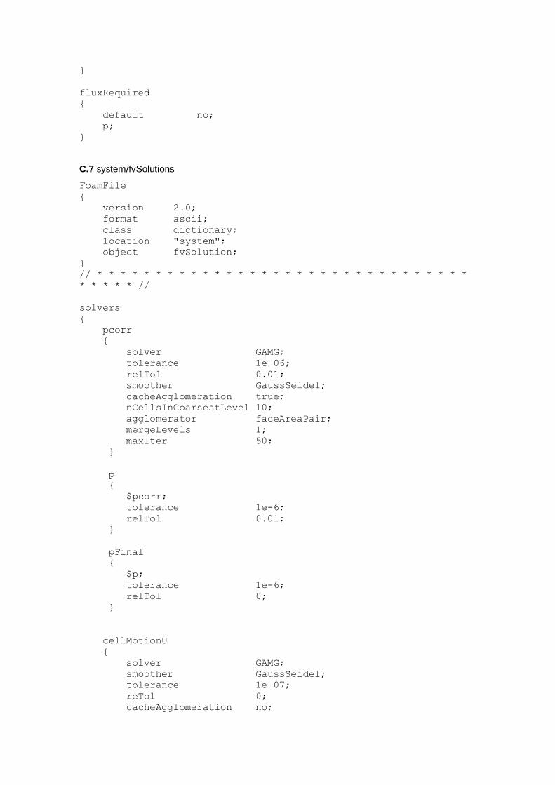
}
fluxRequired
{
default no;
p;
}
C.7 system/fvSolutions
FoamFile
{
version 2.0;
format ascii;
class dictionary;
location "system";
object fvSolution;
}
// * * * * * * * * * * * * * * * * * * * * * * * * * * * * * * * *
* * * * * //
solvers
{
pcorr
{
solver GAMG;
tolerance 1e-06;
relTol 0.01;
smoother GaussSeidel;
cacheAgglomeration true;
nCellsInCoarsestLevel 10;
agglomerator faceAreaPair;
mergeLevels 1;
maxIter 50;
}
p
{
$pcorr;
tolerance 1e-6;
relTol 0.01;
}
pFinal
{
$p;
tolerance 1e-6;
relTol 0;
}
cellMotionU
{
solver GAMG;
smoother GaussSeidel;
tolerance 1e-07;
reTol 0;
cacheAgglomeration no;
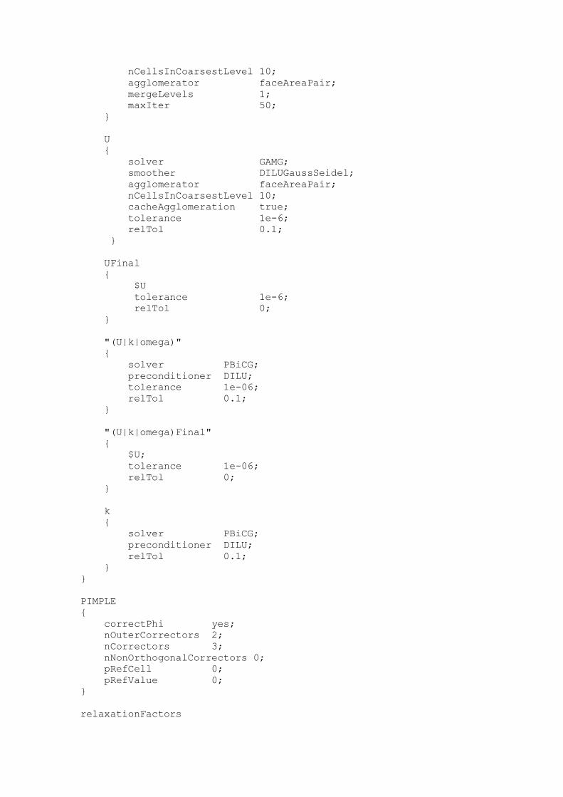
nCellsInCoarsestLevel 10;
agglomerator faceAreaPair;
mergeLevels 1;
maxIter 50;
}
U
{
solver GAMG;
smoother DILUGaussSeidel;
agglomerator faceAreaPair;
nCellsInCoarsestLevel 10;
cacheAgglomeration true;
tolerance 1e-6;
relTol 0.1;
}
UFinal
{
$U
tolerance 1e-6;
relTol 0;
}
"(U|k|omega)"
{
solver PBiCG;
preconditioner DILU;
tolerance 1e-06;
relTol 0.1;
}
"(U|k|omega)Final"
{
$U;
tolerance 1e-06;
relTol 0;
}
k
{
solver PBiCG;
preconditioner DILU;
relTol 0.1;
}
}
PIMPLE
{
correctPhi yes;
nOuterCorrectors 2;
nCorrectors 3;
nNonOrthogonalCorrectors 0;
pRefCell 0;
pRefValue 0;
}
relaxationFactors

{
fields
{
}
equations
{
"U.*" 1;
"p.*" 1;
"omega.*" 1;
}
}
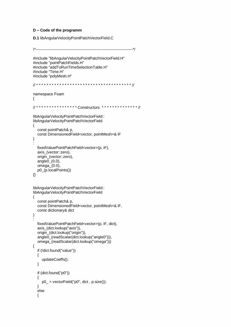
D – Code of the programm
D.1 libAngularVelocityPointPatchVectorField.C
\*---------------------------------------------------------------------------*/ #include "libAngularVelocityPointPatchVectorField.H" #include "pointPatchFields.H" #include "addToRunTimeSelectionTable.H" #include "Time.H" #include "polyMesh.H" // * * * * * * * * * * * * * * * * * * * * * * * * * * * * * * * * * * * * * // namespace Foam { // * * * * * * * * * * * * * * * * Constructors * * * * * * * * * * * * * * // libAngularVelocityPointPatchVectorField:: libAngularVelocityPointPatchVectorField ( const pointPatch& p, const DimensionedField<vector, pointMesh>& iF ) : fixedValuePointPatchField<vector>(p, iF), axis_(vector::zero), origin_(vector::zero), angle0_(0.0), omega_(0.0), p0_(p.localPoints()) {} libAngularVelocityPointPatchVectorField:: libAngularVelocityPointPatchVectorField ( const pointPatch& p, const DimensionedField<vector, pointMesh>& iF, const dictionary& dict ) : fixedValuePointPatchField<vector>(p, iF, dict), axis_(dict.lookup("axis")), origin_(dict.lookup("origin")), angle0_(readScalar(dict.lookup("angle0"))), omega_(readScalar(dict.lookup("omega"))) { if (!dict.found("value")) { updateCoeffs(); } if (dict.found("p0")) { p0_ = vectorField("p0", dict , p.size()); } else {
p0_ = p.localPoints(); } } libAngularVelocityPointPatchVectorField:: libAngularVelocityPointPatchVectorField ( const libAngularVelocityPointPatchVectorField& ptf, const pointPatch& p, const DimensionedField<vector, pointMesh>& iF, const pointPatchFieldMapper& mapper ) : fixedValuePointPatchField<vector>(ptf, p, iF, mapper), axis_(ptf.axis_), origin_(ptf.origin_), angle0_(ptf.angle0_), omega_(ptf.omega_), p0_(ptf.p0_) {} libAngularVelocityPointPatchVectorField:: libAngularVelocityPointPatchVectorField ( const libAngularVelocityPointPatchVectorField& ptf, const DimensionedField<vector, pointMesh>& iF ) : fixedValuePointPatchField<vector>(ptf, iF), axis_(ptf.axis_), origin_(ptf.origin_), angle0_(ptf.angle0_), omega_(ptf.omega_), p0_(ptf.p0_) {} // * * * * * * * * * * * * * * * Member Functions * * * * * * * * * * * * * // void libAngularVelocityPointPatchVectorField::updateCoeffs() { if (this->updated()) { return; } const polyMesh& mesh = this->dimensionedInternalField().mesh()(); const Time& t = mesh.time(); const pointPatch& p = this->patch(); scalar angle = angle0_ + omega_*t.value(); vector axisHat = axis_/mag(axis_); vectorField p0Rel = p0_ - origin_; vectorField::operator= ( ( p0_
+ p0Rel*(cos(angle) - 1) + (axisHat ^ p0Rel*sin(angle)) + (axisHat & p0Rel)*(1 - cos(angle))*axisHat - p.localPoints() )/t.deltaT().value() ); fixedValuePointPatchField<vector>::updateCoeffs(); } void libAngularVelocityPointPatchVectorField::write ( Ostream& os ) const { pointPatchField<vector>::write(os); os.writeKeyword("axis") << axis_ << token::END_STATEMENT << nl; os.writeKeyword("origin") << origin_ << token::END_STATEMENT << nl; os.writeKeyword("angle0") << angle0_ << token::END_STATEMENT << nl; os.writeKeyword("omega") << omega_ << token::END_STATEMENT << nl; p0_.writeEntry("p0", os); writeEntry("value", os); } // * * * * * * * * * * * * * * * * * * * * * * * * * * * * * * * * * * * * * // makePointPatchTypeField ( pointPatchVectorField, libAngularVelocityPointPatchVectorField ); // * * * * * * * * * * * * * * * * * * * * * * * * * * * * * * * * * * * * * // } // End namespace Foam // ************************************************************************* //
D.2 libAngularVelocityPointPatchVectorField.H
Class Foam::libAngularVelocityPointPatchVectorField Description Foam::libAngularVelocityPointPatchVectorField SourceFiles libAngularVelocityPointPatchVectorField.C \*---------------------------------------------------------------------------*/ #ifndef libAngularVelocityPointPatchVectorField_H #define libAngularVelocityPointPatchVectorField_H
#include "fixedValuePointPatchField.H" // * * * * * * * * * * * * * * * * * * * * * * * * * * * * * * * * * * * * * // namespace Foam { /*---------------------------------------------------------------------------*\ Class libAngularVelocityPointPatchVectorField Declaration \*---------------------------------------------------------------------------*/ class libAngularVelocityPointPatchVectorField : public fixedValuePointPatchField<vector> { // Private data vector axis_; vector origin_; scalar angle0_; scalar omega_; pointField p0_; public: //- Runtime type information TypeName("libAngularVelocity"); // Constructors //- Construct from patch and internal field libAngularVelocityPointPatchVectorField ( const pointPatch&, const DimensionedField<vector, pointMesh>& ); //- Construct from patch, internal field and dictionary libAngularVelocityPointPatchVectorField ( const pointPatch&, const DimensionedField<vector, pointMesh>&, const dictionary& ); //- Construct by mapping given patchField<vector> onto a new patch libAngularVelocityPointPatchVectorField ( const libAngularVelocityPointPatchVectorField&, const pointPatch&, const DimensionedField<vector, pointMesh>&, const pointPatchFieldMapper& ); //- Construct and return a clone virtual autoPtr<pointPatchField<vector> > clone() const {
return autoPtr<pointPatchField<vector> > ( new libAngularVelocityPointPatchVectorField ( *this ) ); } //- Construct as copy setting internal field reference libAngularVelocityPointPatchVectorField ( const libAngularVelocityPointPatchVectorField&, const DimensionedField<vector, pointMesh>& ); //- Construct and return a clone setting internal field reference virtual autoPtr<pointPatchField<vector> > clone ( const DimensionedField<vector, pointMesh>& iF ) const { return autoPtr<pointPatchField<vector> > ( new libAngularVelocityPointPatchVectorField ( *this, iF ) ); } // Member functions // Evaluation functions //- Update the coefficients associated with the patch field virtual void updateCoeffs(); //- Write virtual void write(Ostream&) const; }; // * * * * * * * * * * * * * * * * * * * * * * * * * * * * * * * * * * * * * // } // End namespace Foam // * * * * * * * * * * * * * * * * * * * * * * * * * * * * * * * * * * * * * // #endif
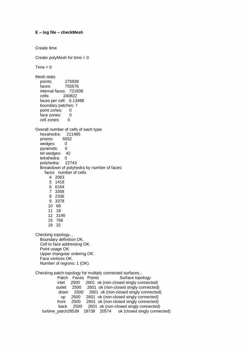
E – log file – checkMesh
Create time Create polyMesh for time = 0 Time = 0 Mesh stats points: 275939 faces: 755576 internal faces: 721838 cells: 240822 faces per cell: 6.13488 boundary patches: 7 point zones: 0 face zones: 0 cell zones: 0 Overall number of cells of each type: hexahedra: 211485 prisms: 6552 wedges: 0 pyramids: 0 tet wedges: 42 tetrahedra: 0 polyhedra: 22743 Breakdown of polyhedra by number of faces: faces number of cells 4 2063 5 1418 6 6164 7 3358 8 2336 9 3378 10 68 11 18 12 3140 15 768 18 32 Checking topology... Boundary definition OK. Cell to face addressing OK. Point usage OK. Upper triangular ordering OK. Face vertices OK. Number of regions: 1 (OK). Checking patch topology for multiply connected surfaces... Patch Faces Points Surface topology inlet 2500 2601 ok (non-closed singly connected) outlet 2500 2601 ok (non-closed singly connected) down 2500 2601 ok (non-closed singly connected) up 2500 2601 ok (non-closed singly connected) front 2500 2601 ok (non-closed singly connected) back 2500 2601 ok (non-closed singly connected) turbine_patch28539 18738 20574 ok (closed singly connected)

Checking geometry... Overall domain bounding box (-15 -15 -15) (15 15 15) Mesh (non-empty, non-wedge) directions (1 1 1) Mesh (non-empty) directions (1 1 1) Boundary openness (-8.78672e-16 3.10042e-17 -1.2724e-16) OK. Max cell openness = 8.3837e-16 OK. Max aspect ratio = 13.9185 OK. Minimum face area = 0.000880194. Maximum face area = 0.411711. Face area magnitudes OK. Min volume = 8.75044e-05. Max volume = 0.236188. Total volume = 26890. Cell volumes OK. Mesh non-orthogonality Max: 59.9817 average: 9.02038 Non-orthogonality check OK. Face pyramids OK. Max skewness = 1.42542 OK. Coupled point location match (average 0) OK. Mesh OK. End