faculdade de ciÊncias e tecnologia · faculdade de ciÊncias e tecnologia departamento de...
TRANSCRIPT

UNIVERSIDADE DE COIMBRAFACULDADE DE CIÊNCIAS E TECNOLOGIA
DEPARTAMENTO DE ENGENHARIA ELECTROTÉCNICA E DE COMPUTADORES
Parallel Algorithms andArchitectures for LDPC Decoding
Gabriel Falcão Paiva Fernandes
(Mestre)
Dissertação para a obtenção do grau de Doutor em
Engenharia Electrotécnica e de Computadores
Dissertação de Doutoramento na área científica de EngenhariaElectrotécnica e de Computadores, especialidade Telecomunicações
e Electrónica, orientada pelo Doutor Leonel Augusto Pires Seabra de Sousado IST/UTL e pelo Doutor Vitor Manuel Mendes da Silva da FCTUC, e apresentada
ao Departamento de Engenharia Electrotécnica e de Computadores da Faculdadede Ciências e Tecnologia da Universidade de Coimbra.
Coimbra
Julho de 2010


Because we live in a parallel world, my graduate studies and in particular this thesishave seen many other persons participating actively, to whom I would like to thank. To
my mother and father for having dedicated full priority to my education and inparticular to my father, who has first shown me the importance and power of
mathematics. To my brother who, accidentally, a few years ago, has found a newspaperannouncing a TA position at the University of Coimbra (UC). I’d also like to thank
father-, brother- and sisters-in-law who have been a friendly presence during myperiods of absence at work, and in particular to M. Ramos who daily helped with the
kids during this turbulent period. And to my wife, Gui, who has guided the shipthrough the storm with perseverance and enthusiasm during a three-year journey.
I thank colleagues M. Gomes for active collaboration over the last years and M. Falcãofor having read parts of this text. Working with my students has been highly
motivating, namely with (in seniority order) P. Ricardo Jesus, J. Cacheira, J. Gonçalves,V. Ferreira, A. Sengo, L. Silva, N. Marques, J. Marinho, A. Carvalho and J. Andrade. I
thank them all. In the SiPS Group at INESC-ID, I would like to express my gratitudeto S. Yamagiwa, D. Antão, N. Sebastião, S. Momcilovic and F. Pratas with whom I
have worked. I’m also grateful to Professor T. Martinez (INESC Coimbra/UC) and P.Tomás (INESC-ID/IST) for the support with LaTeX. Four other persons had a very
important role in my life while I was an undergraduate student at FEUP, and they are:S. Crisóstomo, N. Pinto, L. G. Martins and M. Falcão. I am also grateful to ProfessorAníbal Ferreira (FEUP) who has introduced me in the world of signal processing and
to Professor F. Perdigão (UC) for many enthusiastic discussions and advices. This workhas been possible also thanks to the financial support of the Instituto de
Telecomunicações (IT), INESC-ID and the Portuguese Foundation for Science andTechnology (FCT) under grant SFRH/BD/37495/2007.
Professors Leonel Sousa from INESC-ID and Instituto Superior Técnico (IST) at theTechnical University of Lisbon (TUL) and Vítor Silva from IT and Faculty of Sciences
and Technology of the University of Coimbra (FCTUC), both at the respectiveDepartments of Electrical and Computer Engineering, have supervised this thesis
thoroughly. I thank them guidance and support, and for teaching me the fundamentalsof computer science, parallel computing architectures, VLSI, coding theory and also the
arts of writing. Their vision was essential to maintain the objectives in clear view.


To Guida, Leonor and Francisca

Abstract
Low-Density Parity-Check (LDPC) codes have recaptured the attention of the scien-
tific community a few years after Turbo codes were invented in the early nineties. Origi-
nally proposed in the 1960s at MIT by R. Gallager, LDPC codes represent powerful error
correcting codes that allow working very close to the Shannon limit and achieve excel-
lent Bit Error Rate (BER) due to computationally intensive algorithms on the decoder
side of the system. Advances in microelectronics introduced small process technologies
that allowed developing complex designs incorporating a high number of transistors in
Very Large Scale Integration (VLSI) systems. Recently, these processes have been used
to develop architectures able of performing LDPC decoding in real-time and deliver-
ing considerably high throughputs. Mainly for these reasons and naturally because the
patent has expired, they have been adopted by modern communication standards which
triggered their popularity, showing how actual they are.
Due to the increase of transistor density in VLSI systems, and also to the fact that re-
cently processing speed has risen faster than bandwidth, power and memory walls have
created a new paradigm in computer architectures: rather than just increasing the fre-
quency of operation supported by smaller process designs, the introduction of multiple
cores on a single chip has become the new trend to provide augmented computational
power. This thesis proposes new approaches for these computationally intensive algo-
rithms, by performing parallel LDPC decoding based on ubiquitous multi-core architec-
tures and achieves efficient throughputs that compare well with dedicated VLSI systems.
We extensively address the challenges faced in the investigation and development of
these programmable solutions, with focus mainly given on flexibility and scalability of
the proposed algorithms, throughput and BER performance, and general efficiency of
the programmable solutions here presented, that also achieve results more than an or-
der of magnitude superior to those obtained with conventional CPUs. Furthermore, the
investigation herein described follows a methodology that analyzes in detail the compu-
tational complexity of these decoding algorithms in order to propose strategies to acceler-
ate their processing which, if conveniently transposed to other areas of computer science,
can demonstrate that in this new multi-core era we may be in the presence of valid al-
v

ternatives to non-reprogrammable dedicated VLSI hardware that requires non-recurring
engineering.
Keywords
Parallel computing, Computer architectures, LDPC, Error correcting codes, Multi-
cores, GPU, CUDA, Caravela, Cell/B.E., HPC, OpenMP, Data-parallelism, ILP, HPC,
VLSI, ASIC, FPGA.
vi

Resumo
Os códigos LDPC despertaram novamente a atenção da comunidade científica poucos
anos após a invenção dos Turbo códigos na década de 90. Inventados no MIT por R.
Gallager no início da década de 60, os códigos LDPC representam sistemas correctores
de erros poderosos que permitem trabalhar muito perto do limite de Shannon e obter
taxas de bits errados (BER) excelentes, através da exploração apropriada de algoritmos
computacionalmente intensivos no lado do descodificador do sistema. Avanços recentes
na área da microelectrónica introduziram tecnologias e processos capazes de suportar o
desenvolvimento de sistemas complexos que incorporam um número elevado de transís-
tores em sistemas VLSI. Recentemente, essas tecnologias permitiram o desenvolvimento
de arquitecturas capazes de processar a descodificação de códigos LDPC em tempo-real,
obtendo taxas de débito de saída consideravelmente elevadas. Principalmente por estes
motivos, e também devido ao facto do prazo de validade da patente ter expirado, estes
códigos têm sido adoptados por normas de comunicações recentes, o que comprova a
sua popularidade e actualidade.
Devido ao aumento da densidade de transístores em sistemas microelectrónicos (VLSI),
e uma vez que nos tempos mais recentes a velocidade de processamento tem sofrido uma
evolução mais rápida do que a velocidade de acesso à memória, os problemas associados
à dissipação de potência e a tempos de latência elevados criaram um novo paradigma
em arquitecturas de computadores: ao invés de apenas se privilegiar o aumento da fre-
quência de operação suportada pelo uso de tecnologias que garantem tempos de comu-
tação do transístor cada vez mais reduzidos, a introdução de múltiplas unidades de pro-
cessamento (cores) num único sistema microelectrónico (chip) tornou-se a nova tendên-
cia, mantendo como objectivo principal o contínuo aumento da capacidade de processa-
mento de dados em sistemas de computação. Esta tese propõe novas abordagens para
estes algoritmos de computação intensiva, que permitem realizar o processamento par-
alelo de descodificadores LDPC de forma eficiente baseada em arquitecturas multi-core,
e que conduzem à obtenção de taxas de débito de saída elevadas, comparáveis às obtidas
em sistemas microelectrónicos dedicados (VLSI). É feita a análise exaustiva dos desafios
que se colocam à investigação deste tipo de soluções programáveis, dando-se especial
vii

ênfase à flexibilidade e escalabilidade dos algoritmos propostos, aos níveis da taxa de
débito e taxa de erros (BER) alcançados, bem como à eficiência geral das soluções pro-
gramáveis apresentadas, que alcançam resultados acima de uma ordem de grandeza su-
periores aos obtidos usando CPUs convencionais. Além do mais, a investigação descrita
nesta tese segue uma metodologia que analisa com detalhe a complexidade computa-
cional destes algoritmos de descodificação de modo a propor estratégias de aceleração
do processamento que, se adequadamente transpostas para outros domínios das ciências
da computação, podem demonstrar que nesta nova era dos sistemas multi-core podemos
estar na presença de alternativas viáveis em relação a soluções de hardware dedicado
(VLSI) não reprogramáveis, cujo desenvolvimento envolve um consumo significativo de
recursos não reutilizáveis.
Palavras Chave
Computação paralela, Arquitecturas de computadores, LDPC, Códigos correctores de
erros, Sistemas multi-core, GPU, CUDA, Caravela, Cell/B.E., HPC, OpenMP, Paralelismo
de dados, ILP, HPC, VLSI, ASIC, FPGA.
viii
Contents
1 Introduction 3
1.1 Motivation . . . . . . . . . . . . . . . . . . . . . . . . . . . . . . . . . . . . . 4
1.2 Objectives . . . . . . . . . . . . . . . . . . . . . . . . . . . . . . . . . . . . . 6
1.3 Main contributions . . . . . . . . . . . . . . . . . . . . . . . . . . . . . . . . 8
1.4 Outline . . . . . . . . . . . . . . . . . . . . . . . . . . . . . . . . . . . . . . . 10
2 Overview of Low-Density Parity-Check codes 15
2.1 Binary linear block codes . . . . . . . . . . . . . . . . . . . . . . . . . . . . . 16
2.2 Code generator matrix G . . . . . . . . . . . . . . . . . . . . . . . . . . . . . 17
2.3 Parity-check matrix H . . . . . . . . . . . . . . . . . . . . . . . . . . . . . . 18
2.4 Low-Density Parity-Check codes . . . . . . . . . . . . . . . . . . . . . . . . 18
2.5 Codes on graphs . . . . . . . . . . . . . . . . . . . . . . . . . . . . . . . . . 19
2.5.1 Belief propagation and iterative decoding . . . . . . . . . . . . . . . 20
2.5.2 The Sum-Product algorithm . . . . . . . . . . . . . . . . . . . . . . . 23
2.5.3 The Min-Sum algorithm . . . . . . . . . . . . . . . . . . . . . . . . . 25
2.6 Challenging LDPC codes for developing efficient LDPC decoding solutions 28
2.6.1 LDPC codes for WiMAX (IEEE 802.16e) . . . . . . . . . . . . . . . . 28
2.6.2 LDPC codes for DVB-S2 . . . . . . . . . . . . . . . . . . . . . . . . . 30
2.7 Summary . . . . . . . . . . . . . . . . . . . . . . . . . . . . . . . . . . . . . . 32
3 Computational analysis of LDPC decoding 35
3.1 Computational properties of LDPC decoding algorithms . . . . . . . . . . 36
3.1.1 Analysis of memory accesses and computational complexity . . . . 36
3.1.2 Analysis of data precision in LDPC decoding . . . . . . . . . . . . . 40
3.1.3 Analysis of data-dependencies and data-locality in LDPC decoding 41
3.2 Parallel processing . . . . . . . . . . . . . . . . . . . . . . . . . . . . . . . . 44
3.2.1 Parallel computational approaches . . . . . . . . . . . . . . . . . . . 44
3.2.2 Algorithm parallelization . . . . . . . . . . . . . . . . . . . . . . . . 46
3.2.3 Evaluation metrics . . . . . . . . . . . . . . . . . . . . . . . . . . . . 49
3.3 Parallel algorithms for LDPC decoding . . . . . . . . . . . . . . . . . . . . 50
ix

Contents
3.3.1 Exploiting task and data parallelism for LDPC decoding . . . . . . 50
3.3.2 Message-passing schedule for parallelizing LDPC decoding . . . . 52
3.3.3 Memory access constraints . . . . . . . . . . . . . . . . . . . . . . . 57
3.4 Analysis of the main features of parallel LDPC algorithms . . . . . . . . . 61
3.4.1 Memory-constrained scaling . . . . . . . . . . . . . . . . . . . . . . 61
3.4.2 Scalability of parallel LDPC decoders . . . . . . . . . . . . . . . . . 62
3.5 Summary . . . . . . . . . . . . . . . . . . . . . . . . . . . . . . . . . . . . . . 63
4 LDPC decoding on VLSI architectures 67
4.1 Parallel LDPC decoder VLSI architectures . . . . . . . . . . . . . . . . . . . 68
4.2 A parallel M-kernel LDPC decoder architecture for DVB-S2 . . . . . . . . . 72
4.3 M-factorizable LDPC decoder for DVB-S2 . . . . . . . . . . . . . . . . . . . 75
4.3.1 Functional units . . . . . . . . . . . . . . . . . . . . . . . . . . . . . . 78
4.3.2 Synthesis for FPGA . . . . . . . . . . . . . . . . . . . . . . . . . . . . 80
4.3.3 Synthesis for ASIC . . . . . . . . . . . . . . . . . . . . . . . . . . . . 83
4.4 Optimizing RAM memory design for ASIC . . . . . . . . . . . . . . . . . . 85
4.4.1 Minimal RAM memory configuration . . . . . . . . . . . . . . . . . 87
4.4.2 ASIC synthesis results for an optimized 45 FUs architecture . . . . 89
4.5 Summary . . . . . . . . . . . . . . . . . . . . . . . . . . . . . . . . . . . . . . 92
5 LDPC decoding on multi- and many-core architectures 97
5.1 Multi-core architectures and parallel programming technologies . . . . . . 99
5.2 Parallel programming strategies and platforms . . . . . . . . . . . . . . . . 103
5.2.1 General-purpose x86 multi-cores . . . . . . . . . . . . . . . . . . . . 103
5.2.2 The Cell/B.E. from Sony/Toshiba/IBM . . . . . . . . . . . . . . . . 103
5.2.3 Generic processing on GPUs with Caravela . . . . . . . . . . . . . . 105
5.2.4 NVIDIA graphics processing units with CUDA . . . . . . . . . . . 108
5.3 Stream computing LDPC kernels . . . . . . . . . . . . . . . . . . . . . . . . 109
5.4 LDPC decoding on general-purpose x86 multi-cores . . . . . . . . . . . . . 111
5.4.1 OpenMP parallelism on general-purpose CPUs . . . . . . . . . . . 111
5.4.2 Experimental results with OpenMP . . . . . . . . . . . . . . . . . . 112
5.5 LDPC decoding on the Cell/B.E. architecture . . . . . . . . . . . . . . . . . 114
5.5.1 The small memory model . . . . . . . . . . . . . . . . . . . . . . . . 115
5.5.2 The large memory model . . . . . . . . . . . . . . . . . . . . . . . . 117
5.5.3 Experimental results for regular codes with the Cell/B.E. . . . . . . 121
5.5.4 Experimental results for irregular codes with the Cell/B.E. . . . . . 126
5.6 LDPC decoding on GPU-based architectures . . . . . . . . . . . . . . . . . 127
5.6.1 LDPC decoding on the Caravela platform . . . . . . . . . . . . . . . 128
x

Contents
5.6.2 Experimental results with Caravela . . . . . . . . . . . . . . . . . . 132
5.6.3 LDPC decoding on CUDA-based platforms . . . . . . . . . . . . . . 134
5.6.4 Experimental results for regular codes with CUDA . . . . . . . . . 138
5.6.5 Experimental results for irregular codes with CUDA . . . . . . . . 143
5.7 Discussion of architectures and models for parallel LDPC decoding . . . . 145
5.8 Summary . . . . . . . . . . . . . . . . . . . . . . . . . . . . . . . . . . . . . . 147
6 Closure 151
6.1 Future work . . . . . . . . . . . . . . . . . . . . . . . . . . . . . . . . . . . . 154
A Factorizable LDPC Decoder Architecture for DVB-S2 159
A.1 M parallel processing units . . . . . . . . . . . . . . . . . . . . . . . . . . . 160
A.1.1 Memory mapping and shuffling mechanism . . . . . . . . . . . . . 161
A.2 Decoding decomposition by a factor of M . . . . . . . . . . . . . . . . . . . 162
A.2.1 Memory mapping and shuffling mechanism . . . . . . . . . . . . . 163
xi

Contents
xii

List of Figures
1.1 Proposed approaches and technologies that support the LDPC decoders
presented in this thesis. . . . . . . . . . . . . . . . . . . . . . . . . . . . . . . 11
2.1 A (8, 4) linear block code example: parity-check equations, the equivalent
H matrix and corresponding Tanner graph [118] representation. . . . . . . . 20
2.2 Illustration of channel coding for a communication system. . . . . . . . . . 21
2.3 Detail of a check node update by the bit node connected to it as defined
in the Tanner graph for the example shown in figure 2.5. It represents the
calculation of qnm(x) probabilities given by (2.16). . . . . . . . . . . . . . . 22
2.4 Detail of a bit node update by the constraint check node connected to it
as defined in the Tanner graph for the example depicted in figure 2.5. It
represents the calculation of rmn(x) probabilities given by (2.17). . . . . . . 23
2.5 Tanner graph [118] expansion showing the iterative decoding procedure for
the code shown in figure 2.1. . . . . . . . . . . . . . . . . . . . . . . . . . . . 24
2.6 Periodicity z× z = 96× 96 for an H matrix with N = 2304, rate = 1/2 and
{3, 6} CNs per column. . . . . . . . . . . . . . . . . . . . . . . . . . . . . . . 29
3.1 Mega operations (MOP) per iteration for 5 distinct H matrices (A to E),
with a) wc = 6 and wb = 3; and b) wc = 14 and wb = 6. . . . . . . . . . . . 39
3.2 Giga operations (GOP) for the parallel decoding of 1000 codewords run-
ning 15 iterations each, for the same H matrices referred in figure 3.1, with
a) wc = 6 and wb = 3; and b) wc = 14 and wb = 6. . . . . . . . . . . . . . . 40
3.3 Average number of iterations per SNR, comparing 8-bit and 6-bit data pre-
cision representations for WiMAX LDPC codes (576,288) and (1248,624) [64]
running a maximum of 50 iterations. . . . . . . . . . . . . . . . . . . . . . . 41
3.4 BER curves comparing 8-bit and 6-bit data precision for WiMAX LDPC
codes (576,288) and (1248,624) [64]. . . . . . . . . . . . . . . . . . . . . . . . . 42
3.5 Finding concurrency design space adapted from [25] to incorporate schedul-
ing. . . . . . . . . . . . . . . . . . . . . . . . . . . . . . . . . . . . . . . . . . 48
3.6 Task and data-parallelism . . . . . . . . . . . . . . . . . . . . . . . . . . . . 51
xiii
List of Figures
3.7 Flooding schedule approach. . . . . . . . . . . . . . . . . . . . . . . . . . . 53
3.8 Horizontal schedule approach. . . . . . . . . . . . . . . . . . . . . . . . . . 54
3.9 Horizontal block schedule approach. . . . . . . . . . . . . . . . . . . . . . . 54
3.10 Vertical scheduling approach. . . . . . . . . . . . . . . . . . . . . . . . . . . 55
3.11 Vertical block scheduling approach. . . . . . . . . . . . . . . . . . . . . . . 56
3.12 Data structures illustrating the Tanner graph’s irregular memory access
patterns for the example shown in figures 2.1 and 2.5. . . . . . . . . . . . . 58
3.13 a) HCN and b) HBN generic data structures developed, illustrating the Tan-
ner graph’s irregular memory access patterns. . . . . . . . . . . . . . . . . 60
3.14 Irregular memory access patterns for BN0 and CN0. . . . . . . . . . . . . . 61
4.1 Generic parallel LDPC decoder architecture [1] based on node processors
with associated memory banks and interconnection network (usually, P =
Q). . . . . . . . . . . . . . . . . . . . . . . . . . . . . . . . . . . . . . . . . . . 69
4.2 Parallel architecture with M functional units (FU) [51,70]. . . . . . . . . . . . 73
4.3 Memory organization for the computation of Lrmn and Lqnm messages us-
ing M = 360 functional units for a Digital Video Broadcasting – Satellite
2 (DVB-S2) LDPC code with q = (N − K)/M (see table 2.3). . . . . . . . . 74
4.4 M-factorizable architecture [51]. . . . . . . . . . . . . . . . . . . . . . . . . . 75
4.5 Memory organization for the computation of Lrmn and Lqnm messages, au-
tomatically adapted for a L = 2 factorizable architecture with correspond-
ing P = 180 functional units, for the example shown in figure 4.3. . . . . . 76
4.6 Serial architecture for a functional unit that supports both CN and BN pro-
cessing types [31,49] for the MSA. . . . . . . . . . . . . . . . . . . . . . . . . . 77
4.7 Boxplus and boxminus sub-architectures of figure 4.6 [31,49]. . . . . . . . . . 78
4.8 Parallel architecture for a functional unit that supports both CN and BN
processing types [31,49] for the MSA. . . . . . . . . . . . . . . . . . . . . . . . 79
4.9 Maximum number of iterations . . . . . . . . . . . . . . . . . . . . . . . . . 82
4.10 Minimum throughput . . . . . . . . . . . . . . . . . . . . . . . . . . . . . . 83
4.11 Area results for ASIC architectures with P = {360, 180, 90, 45} functional
units. . . . . . . . . . . . . . . . . . . . . . . . . . . . . . . . . . . . . . . . . 84
4.12 Tiling of an y (height) by x (width) RAM memory layout. . . . . . . . . . . 87
4.13 Optimized 45 functional units architecture. . . . . . . . . . . . . . . . . . . 88
4.14 Layout of a memory with 10-bit width ×10 lines of bus address. . . . . . . 89
4.15 Floorplan with placed std cells, RAM and pins for the optimized 45 func-
tional units design. . . . . . . . . . . . . . . . . . . . . . . . . . . . . . . . . 90
4.16 Area results comparing the optimized 45 FUs design. . . . . . . . . . . . . 90
xiv

List of Figures
4.17 Reference designs for gate count comparison of the Application Specific In-
tegrated Circuits (ASIC) based architectures proposed, with 360, 180, 90, 45
and 45-optimized functional units. . . . . . . . . . . . . . . . . . . . . . . . 91
5.1 The Cell/B.E. architecture. . . . . . . . . . . . . . . . . . . . . . . . . . . . . 104
5.2 Double buffering showing the use of the two pipelines (for computation
and DMA). . . . . . . . . . . . . . . . . . . . . . . . . . . . . . . . . . . . . . 104
5.3 Vertex and pixel processing pipeline for GPU computation [126]. . . . . . . 105
5.4 A GPU processing pipeline with Caravela. . . . . . . . . . . . . . . . . . . 106
5.5 Structure of Caravela’s flow-model. . . . . . . . . . . . . . . . . . . . . . . 107
5.6 A compute unified Tesla GPU architecture with 8 stream processors (SP)
per multiprocessor. . . . . . . . . . . . . . . . . . . . . . . . . . . . . . . . . 108
5.7 SDF graph for a stream-based LDPC decoder: the pair kernel 1 and ker-
nel 2 is repeated i times for an LDPC decoder performing i iterations. . . . 110
5.8 Detail of the parallelization model developed for the simultaneous decod-
ing of several codewords using SIMD instructions. . . . . . . . . . . . . . . 115
5.9 Parallel LDPC decoder on the Cell/B.E. architecture running the small
memory model. . . . . . . . . . . . . . . . . . . . . . . . . . . . . . . . . . . 116
5.10 Parallel LDPC decoder on the Cell/B.E. architecture running the large mem-
ory model. . . . . . . . . . . . . . . . . . . . . . . . . . . . . . . . . . . . . . 119
5.11 LDPC decoding times per codeword for sequential and parallel modes on
the Cell/B.E., running the SPA with regular codes in the small model (ms) 123
5.12 Model bounds for execution times obtained on the Cell/B.E. . . . . . . . . 125
5.13 2D textures Tn associated to pixel processors Pn in Caravela. . . . . . . . . 128
5.14 HBN structure. A 2D texture representing Bit Node edges with circular
addressing for the example in figure 2.1. Also, the pixel processors entry
points are shown. . . . . . . . . . . . . . . . . . . . . . . . . . . . . . . . . . 130
5.15 HCN structure. A 2D texture representing Check Node edges with circular
addressing for the example in figure 2.1. Also, the pixel processors entry
points are shown. . . . . . . . . . . . . . . . . . . . . . . . . . . . . . . . . . 131
5.16 Organization of the LDPC decoder flow-model. . . . . . . . . . . . . . . . 132
5.17 Decoding times running the SPA on an 8800 GTX GPU from NVIDIA pro-
grammed with Caravela. . . . . . . . . . . . . . . . . . . . . . . . . . . . . . 134
5.18 Detail of tx× ty threads executing on the GPU grid inside a block for ker-
nel 1 (the example refers to figure 3.12 and shows BNs associated to CN0,
CN1 and CN2 being updated). . . . . . . . . . . . . . . . . . . . . . . . . . . 136
xv

List of Figures
5.19 Transformations applied to data structures to support coalesced memory
read operations performed by the 16 threads of a half-warp on a single
memory access. . . . . . . . . . . . . . . . . . . . . . . . . . . . . . . . . . . 137
5.20 Thread execution times for LDPC decoding on the GPU running the SPA. 140
xvi

List of Tables
2.1 Properties of LDPC codes used in the WiMAX IEEE 802.16e standard [64]. . 29
2.2 Properties of short frame DVB-S2 codes . . . . . . . . . . . . . . . . . . . . 31
2.3 Properties of LDPC codes used in the DVB-S2 standard [29] for the normal
frame length. . . . . . . . . . . . . . . . . . . . . . . . . . . . . . . . . . . . . 32
3.1 Number of arithmetic and memory access operations per iteration for the
Sum-Product Algorithm (SPA). . . . . . . . . . . . . . . . . . . . . . . . . . 37
3.2 Number of arithmetic and memory access operations per iteration for the
optimized Forward-and-Backward algorithm [63]. . . . . . . . . . . . . . . . 38
3.3 Number of arithmetic and memory access operations per iteration for the
optimized Min-Sum Algorithm (MSA). . . . . . . . . . . . . . . . . . . . . 39
3.4 Message computations for one iteration of the example shown in figures 2.1
and 2.5. . . . . . . . . . . . . . . . . . . . . . . . . . . . . . . . . . . . . . . . 42
3.5 Steps in the parallelization process. . . . . . . . . . . . . . . . . . . . . . . . 47
4.1 Synthesis results for P={45, 90, 180} parallel functional units . . . . . . . . 81
4.2 Required RAM memory size for each configuration. . . . . . . . . . . . . . 86
4.3 Physical (real) RAM memory size for each configuration. . . . . . . . . . . 86
4.4 ASIC synthesis results for P = {45, 90, 180, 360} parallel functional units
and for an optimized 45 functional units architecture. . . . . . . . . . . . . 91
5.1 Overview of multi-core platforms. . . . . . . . . . . . . . . . . . . . . . . . 100
5.2 Overview of software technologies for multi-cores. . . . . . . . . . . . . . . 102
5.3 Types of parallelism on multi-core platforms. . . . . . . . . . . . . . . . . . 110
5.4 Experimental setup . . . . . . . . . . . . . . . . . . . . . . . . . . . . . . . . 112
5.5 Parity-check matrices H under test for the general-purpose x86 multi-cores 113
5.6 Decoding throughputs running the SPA with regular LDPC codes on x86
multi-cores programming algorithm 5.1 with OpenMP (Mbps) . . . . . . . 113
5.7 Experimental setup for the Cell/B.E. . . . . . . . . . . . . . . . . . . . . . . 121
5.8 Parity-check matrices H under test for the Cell/B.E. . . . . . . . . . . . . . 122
xvii

List of Tables
5.9 Decoding throughputs for a Cell/B.E. programming environment in the
small model running the SPA with regular LDPC codes (Mbps) . . . . . . 123
5.10 Decoding throughputs for a Cell/B.E. programming environment in the
small model running the MSA with irregular WiMAX LDPC codes (Mbps) 127
5.11 Experimental setup for Caravela . . . . . . . . . . . . . . . . . . . . . . . . 133
5.12 Parity-check matrices H under test for Caravela . . . . . . . . . . . . . . . 133
5.13 Experimental setups for the Tesla GPUs with CUDA . . . . . . . . . . . . . 138
5.14 Parity-check matrices H under test for the CUDA . . . . . . . . . . . . . . 138
5.15 LDPC decoding throughputs for a CUDA programming environment run-
ning the SPA with regular codes (Mbps) . . . . . . . . . . . . . . . . . . . . 139
5.16 LDPC decoding times on the GPU (ms) and corresponding throughputs
(Mbps) for an 8-bit data precision solution decoding 16 codewords in par-
allel running the MSA with regular codes. . . . . . . . . . . . . . . . . . . . 141
5.17 LDPC decoding times on the GPU (ms) and corresponding throughputs
(Mbps) for an 8-bit data precision solution decoding 16 codewords in par-
allel running the MSA with irregular DVB-S2 codes. . . . . . . . . . . . . . 144
5.18 Comparing LDPC decoding throughputs for DVB-S2 code t6 running the
MSA with 8- and 16-bit data precision solutions (Mbps) . . . . . . . . . . . 145
5.19 Comparison with state-of-the-art ASIC LDPC decoders using the MSA. . . 146
xviii
List of Algorithms
2.1 Sum-Product Algorithm – SPA . . . . . . . . . . . . . . . . . . . . . . . . . 25
2.2 Min-Sum Algorithm – MSA . . . . . . . . . . . . . . . . . . . . . . . . . . . 27
3.1 Algorithm for the horizontal schedule (sequential). . . . . . . . . . . . . . 53
3.2 Algorithm for the horizontal block schedule (semi-parallel). The architec-
ture supports P processing units and the subset defining the CNs to be
processed in parallel is specified by Φ{.}. . . . . . . . . . . . . . . . . . . . 55
3.3 Generating the compact HBN structure from the original H matrix. . . . . 59
3.4 Generating the compact HCN structure from the original H matrix. . . . . 59
5.1 LDPC kernels executing on general-purpose x86 multi-cores using OpenMP 111
5.2 Multi-codeword LDPC decoding on general-purpose x86 multi-cores us-
ing OpenMP . . . . . . . . . . . . . . . . . . . . . . . . . . . . . . . . . . . . 112
5.3 PPE algorithm in the small memory model . . . . . . . . . . . . . . . . . . 116
5.4 MASTER SPE algorithm in the small memory model . . . . . . . . . . . . 117
5.5 SLAVE SPE algorithm in the small memory model . . . . . . . . . . . . . . 117
5.6 PPE algorithm in the large memory model . . . . . . . . . . . . . . . . . . 120
5.7 SPE algorithm in the large memory model . . . . . . . . . . . . . . . . . . . 121
5.8 Generating compact 2D HBN textures from original H matrix . . . . . . . . 129
5.9 Generating compact 2D HCN textures from original H matrix and HBN . . 130
5.10 GPU algorithm (host side) . . . . . . . . . . . . . . . . . . . . . . . . . . . . 135
xix

List of Algorithms
xx

List of Acronyms
AWGN additive white Gaussian noise
API Application Programming Interface
APP a posteriori probability
AI artificial intelligence
ASIC Application Specific Integrated Circuits
BER Bit Error Rate
BP belief propagation
BPSK Binary Phase Shift Keying
CCS compress column storage
Cell/B.E. Cell Broadband Engine
CPU Central Processing Unit
CRS compress row storage
CTM Close to the metal
CUDA Compute Unified Device Architecture
DMA Direct Memory Access
DSP Digital Signal Processor
DVB-S2 Digital Video Broadcasting – Satellite 2
FEC Forward Error Correcting
FFT Fast Fourier Transform
FPGA Field Programmable Gate Array
xxi
List of Acronyms
FU Functional Units
GLSL OpenGL Shading Language
GPGPU General Purpose Computing on GPUs
GPU Graphics Processing Units
GT Giga Transfer
HDL Hardware Description Language
HLSL High Level Shader Language
IRA Irregular Repeat Accumulate
LDPC Low-Density Parity-Check
LLR Log-likelihood ratio
LS local storage
LSPA Logarithmic Sum-Product Algorithm
MAN Metropolitan Area Networks
MFC Memory Flow Controller
MIC Memory Interface Controller
MIMD Multiple Instruction Multiple Data
MPI Message Passing Interface
MSA Min-Sum Algorithm
NRE Non-Recurring Engineering
NUMA Non-Uniform Memory Architecture
PC Personal Computer
PCIe Peripheral Component Interconnect Express
PS3 PlayStation3
PPE PowerPC Processor Element
QMR Quick Medical Reference
xxii

List of Acronyms
RTL Register Transfer Level
SDR Software Defined Radio
SIMD Single Instruction Multiple Data
SIMT Single Instruction Multiple Thread
SoC System-on-Chip
SNR Signal-to-Noise Ratio
SPA Sum-Product Algorithm
SPE Synergistic Processor Element
SPMD Single Program Multiple Data
SWAR SIMD within-a-register
SDF Synchronous Data Flow
VLDW Very Long Data Word
VLSI Very Large Scale Integration
VRAM video RAM
xxiii

List of Acronyms
xxiv

Mathematical numenclature
Sets
S General SetR Set of real numbers
N Set of natural numbersZ Set of integer numbers
Variables and functions
x Variable
X Constantx Estimated value of variable x
abs(x) The absolute value of a number: |−x| = x
sign(x) Operation that extracts the sign of a number: sign(−x) = −
xor{· · · } Logical Xor function between two or more argumentslog(x) The natural logarithm of x: log(ex) = x
logy(x) The logarithm base y of x: logy(x) = log(y)/ log(x)
min{· · ·} Function that returns the smallest value of the arguments;if the argument is a matrix, it returns the smallest of all ele-ments in the matrix
max{· · ·} Function that returns the largest value of the arguments; ifthe argument is a matrix, it returns the largest of all ele-ments in the matrix
xxv

Mathematical numenclature
Matrix, vectors, and vector functions
x Vector, typically a column vectorX Matrix
000/
111 Matrix where all elements are 0/1000[I×J]
/111[I×J] Matrix with I rows and J columns where all elements are
0/1
(x)i/
xi Element i of vector x
(X)i,j/
Xi,j Element in row i, column j of matrix X
(X)⋆,j Column vector containing the elements of column j of ma-trix X
(X)i,⋆ Row vector containing the elements of row i of matrix X
XT Transpose of matrix X
Statistical operators
v ,x ,y ,z ,... Random variables; v 6= v, x 6= x, y 6= y, z 6= z, ...
P(x = x)/
P(x) Probability for x to be equal to x; the random variable xhas a finite number of states.
p(x = x)/
p(x) Probability density function for x to be equal to x; the ran-dom variable x has an infinite number of states.
p(x = x
∣∣y = y
)/p(x|y) Probability density function for x to be equal to x, given
that (conditioned to) y = y; the random variable x has aninfinite number of states; however, y may or may not havean infinite number of states.
E[x ] Expected value of the random variable xVAR[x ] Variance of the random variable x
N(µ; σ2
)Normal distribution with mean µ and variance σ2.
x ∼ N (µ, σ2) x is distributed according to a normal distribution withmean µ and variance σ2.
xxvi

Há um tempo em que é preciso abandonar as roupas usadas, que já têm a forma donosso corpo, e esquecer os nossos caminhos, que nos levam sempre aos mesmos lugares.
É o tempo da travessia: e, se não ousarmos fazê-la, teremos ficado, para sempre, àmargem de nós mesmos.
Fernando Pessoa

1Introduction
Contents1.1 Motivation . . . . . . . . . . . . . . . . . . . . . . . . . . . . . . . . . . . . 4
1.2 Objectives . . . . . . . . . . . . . . . . . . . . . . . . . . . . . . . . . . . . 6
1.3 Main contributions . . . . . . . . . . . . . . . . . . . . . . . . . . . . . . . 8
1.4 Outline . . . . . . . . . . . . . . . . . . . . . . . . . . . . . . . . . . . . . . 10
3
1. Introduction
1.1 Motivation
Over the last 15 years we have seen Low-Density Parity-Check (LDPC) codes assum-
ing greater and greater importance in the channel coding arena, namely because they
have error correction capability to achieve efficient coding close to the Shannon limit.
They were invented by Robert Gallager (MIT) in the early sixties [46] and never been fully
exploited due to overwhelming computational requirements by that time. Naturally, the
fact that nowadays their patent has expired, has shifted the attention of the scientific com-
munity and industry away from Turbo codes [9,10] towards LDPC codes. Mainly for this
reason and also because advances in microelectronics allowed the development of hard-
ware solutions for real-time LDPC decoding, they have been adopted by modern commu-
nication standards. Important examples of these standards are: the WiMAX IEEE 802.16e
used in wireless communication systems in Metropolitan Area Networks (MAN) [64]; the
Digital Video Broadcasting – Satellite 2 (DVB-S2) used in long distance wireless com-
munications [29]; the WiFi 802.11n the ITU-T G.hn standard for wired home networking
technologies; the 10 Giga-Bit Ethernet IEEE 802.3an; or the 3GPP2 Ultra Mobile Broad-
band (UMB) under the evolution of the 3G mobile system, where the introduction of
LDPC codes in 4G systems has recently been proposed, as opposed to the use of Turbo
codes in 3G.
Until very recently, solutions for LDPC decoding were exclusively based on dedi-
cated hardware such as Application Specific Integrated Circuits (ASIC), which represent
non-flexible and non-reprogrammable approaches [18,70]. Also, the development of ASIC
solutions for LDPC decoding consumes significant resources, with high Non-Recurring
Engineering (NRE) penalty, and presents long development periods (penalizing time-
to-market). An additional restriction in currently developed ASICs for LDPC decoding
is the use of fixed-point arithmetic. This introduces limitations due to quantization ef-
fects [101] that impose restrictions on coding gains, error floors and Bit Error Rate (BER).
Also, the complexity of Very Large Scale Integration (VLSI) parallel LDPC decoders in-
creases significantly for long length codes, as those used, for example, in the DVB-S2
standard. In this case, the routing complexity assumes proportions that create great dif-
ficulties in the design of such architectures.
In recent years, we have seen processors scaling up to hundreds of millions of tran-
sistors. Memory and power walls have shifted the paradigm of computer architectures
into the multi-core era [59]. The integration of multiple cores into a single chip has be-
come the new trend to increase processor performance. Multi-core architectures [12] have
evolved from dual or quad-core to many-core systems, supporting multi-threading, a
powerful technique to hide memory latency, while at the same time provide larger Single
4

1.1 Motivation
Instruction Multiple Data (SIMD) units for vector processing. The number of cores per
processor assumes significant proportions and is expected to increase even further in the
future [16,58]. This new context motivates the investigation of more flexible approaches
based on multi-cores to solve challenging computational problems that require intensive
processing, and that typically were only achieved in the past with VLSI dedicated accel-
erators.
Generally worldwide disseminated, many of the actual parallel computing [12] plat-
forms provide low-cost high-performance massive computation, supported by conve-
nient programming languages, interfaces, tools and libraries [71,89]. The advantages of us-
ing software- versus hardware-based approaches are essentially related with programma-
bility, reconfigurability, scalability and adjustable data-precision. The advantage is clear
if NRE is used as the figure of merit to compare both approaches. However, developing
programs for platforms with multiple cores is not trivial. Exploiting the full potential
of multi-core based computers many times involves expertise on parallel computation
and specific skills which, at the moment, still compel the software developer to deal with
low-level architectural/software details.
In the last decade we have seen a vast set of multi-core architectures emerging [12],
allowing processing performances unmatched before. The general-purpose multi-core
processors replicate a single core in a homogeneous way, typically with a x86 instruction
set, and provide shared memory hardware mechanisms. They support multi-threading
and share data at a certain level of the memory hierarchy, and can be programmed at a
high level by using different software technologies [71]. The popularity of these architec-
tures has made multi-core processing power generally available everywhere.
Mainly due to demands for visualization technology in the games industry, Graphics
Processing Units (GPU) have undergone increasing performances over the last decade.
Even in a commodity personal computer, we now have at disposal high quality graphics
created by real-time computing, mainly due to the high performance GPUs available in
personal computers. With many cores driven by a considerable memory bandwidth and
a shared memory architecture, recent GPUs are targeted for compute-intensive, multi-
threaded, highly-parallel computation, and researchers in high performance computing
fields are exploiting GPUs for General Purpose Computing on GPUs (GPGPU) [20,54,99].
Also pushed by audiovisual needs in the industry of games, emerged the Sony, Toshiba
and IBM (STI) Cell Broadband Engine (Cell/B.E.) Architecture (CBEA) [24] [60]. It is char-
acterized by an heterogeneous vectorized SIMD multi-core architecture composed by one
main PowerPC Processor that communicates efficiently with several Synergistic Proces-
sors. It is based on a distributed memory architecture where fast communications be-
tween processors are supported by high bandwidth dedicated buses.
5

1. Introduction
Motivated by the evolution of these multi-core systems, programmable parallel ap-
proaches for the computationally intensive processing of LDPC decoding are desirable.
Multi-cores can allow a low level of NRE and the flexibility they introduce can be used
to exploit other levels of efficiency. However, many challenges have to be successfully
addressed fostering these approaches, namely the efficiency of data communications and
synchronization between cores, the reduction of latency and minimization of congestion
problems that may occur in parallel memory accesses, cache coherency and memory hi-
erarchy issues, and scalability of the algorithms, just to name a few. The investigation
of efficient parallel algorithms for LDPC decoding has to consider the characteristics of
the different architectures, such as homogeneity or heterogeneity of the parallel architec-
ture, and memory models that can support data sharing or be distributed (models that
exploit both types also exist). The diversity of architectures imposes different strategies
in order to exploit parallelism conveniently. Another important issue consists of adopt-
ing data representations suitable for parallel computing engines. All these aspects have
significant impact on the achieved performance.
The development of programs for the considered parallel computing architectures
allows assessing the performance of software-based solutions for LDPC decoding. The
difficulty of developing accurate models for predicting the computational performance of
these architectures is associated with the existence of a large variety of parameters which
can be manipulated within each architecture. Advances in this area can help understand-
ing how far parallel algorithms are from their theoretical peak performance. This infor-
mation can be used to tune an algorithm’s execution time targeting a certain multi-core
architecture. More importantly, it can be used to help perceiving how compilers and
parallel programming tools should evolve towards the massive exploitation of the full
potential of parallel computing architectures.
1.2 Objectives
Given the many challenges associated with the investigation of novel efficient forms
of performing parallel LDPC decoding, the main objectives of the research work herein
described consist of: i) researching new parallel architectures for VLSI-based LDPC de-
coders under the context of DVB-S2, pursuing the objective of reducing the routing com-
plexity of the design, occupying small die areas and consume low power, while guaran-
teeing high throughputs; ii) investigating novel parallel approaches, algorithms and data
structures for ubiquitous low-cost multi-core processors; iii) deriving parallel kernels for
a set of predefined multi-core architectures based on the proposed algorithms; and iv)
assessing their efficiency against state-of-the-art hardware-based VLSI solutions, namely
6

1.2 Objectives
by comparing throughput and BER performance.
Common general-purpose processors have been used in the research of good LDPC
codes (searching low error floors, while guaranteeing sparsity) and other types of of-
fline processing necessary to investigate the coding gains of LDPC codes, but they have
never been considered for real-time decoding which, depending on the length of the
LDPC code, may produce very intensive workloads. Thus, with these processors it is not
possible to achieve the required throughput for real-time LDPC decoders, and hardware-
dedicated solutions have to be considered.
One of the main objectives of this thesis consisted of investigating more efficient
hardware-dedicated solutions (e. g. based on Field Programmable Gate Array (FPGA)
or ASIC) for DVB-S2 LDPC decoders. The length of codes adopted in this standard is
so large, that actually they represent the most complex challenge regarding the develop-
ment of efficient solutions for VLSI-based LDPC decoders. Under this context, perform-
ing LDPC decoding with a reduced number of light weight node processors, associated
with the possibility of reducing the routing complexity of the interconnection network
that connects processor nodes and memory blocks, is a target that aims to improve the
design in terms of cost and complexity.
While the development of hardware solutions for LDPC decoding was dependent
on VLSI technology, it imposed restrictions at the level of data representation, coding
gains, BER, etc. The advent of the multi-core era encourages the development of new
programmable, flexible and reconfigurable solutions that can represent data with a pro-
grammable number of bits. Under this context, the use of massively disseminated ar-
chitectures with many cores available to solve these computational challenges can be
exploited. In this sense, new parallel approaches and algorithms had to be investigated
and developed to achieve these goals, which represented another of the main objectives
of the thesis.
This led to the development of new forms of representing data to suit parallel com-
puting and stream-based architectures. Since in parallel systems there are multiple cores
performing concurrent accesses to data structures in memory, they may have to obey to
special constraints such as dimension and alignment in appropriate memory addresses
to minimize the problem of traffic congestion. The investigation of these data structures
was motivated by the development of appropriate parallel algorithms.
The variety and heterogeneity of programming models and parallel architectures
available represented a challenge in this research work. A set of parallel computing ma-
chines, selected based on properties such as computational power, popularity, worldwide
dissemination and cost, have been considered to solve the intensive computational prob-
lem of LDPC decoding. Special challenges have to be addressed, such as: irregular data
7

1. Introduction
representation of binary sparse matrices; intensive computation, which requires itera-
tive decoding but exhibits different levels of parallelism to target distinct architectures,
such as homogeneous and heterogeneous systems, with shared and distributed memory.
Also, the inclusion of models to predict the performance of the algorithms developed in
these types of parallel computing architectures represents a difficult problem which can
be tackled by testing separately (and independently) several case limit situations (e.g.
memory accesses, or arithmetic instructions). This thesis also assesses the efficiency of
the proposed software-based LDPC decoders and compares it with dedicated hardware
(e.g. VLSI).
The research carried out, the problems addressed and the solutions developed for the
case of LDPC decoding under the context of this thesis, should preferably be portable
and serve a variety of other types of computationally intensive problems.
1.3 Main contributions
The main contributions of this Ph.D. thesis are:
i) optimization of specific hardware components used in VLSI LDPC decoders for
DVB-S2; simplification of the interconnection network; optimization of synthesis
results for processing units and RAM memory blocks; development of new semi-
parallel, scalable and factorizable architectures; prototyping and testing in FPGA
and ASIC devices; this work has been communicated in:
[31] Falcão, G., Gomes, M., Gonçalves, J., Faia, P., and Silva, V. (2006). HDL Library
of Processing Units for an Automatic LDPC Decoder Design. In Proceedings
of the IEEE Ph.D. Research in Microelectronics and Electronics (PRIME’06), pages
349–352.
[49] Gomes, M., Falcão, G., Gonçalves, J., Faia, P., and Silva, V. (2006a). HDL Li-
brary of Processing Units for Generic and DVB-S2 LDPC Decoding. In Pro-
ceedings of the International Conference on Signal Processing and Multimedia Appli-
cations (SIGMAP’06).
[50] Gomes, M., Falcão, G., Silva, V., Ferreira, V., Sengo, A., and Falcão, M. (2007a).
Factorizable modulo M parallel architecture for DVB-S2 LDPC decoding. In
Proceedings of the 6th Conference on Telecommunications (CONFTELE’07).
[51] Gomes, M., Falcão, G., Silva, V., Ferreira, V., Sengo, A., and Falcão, M. (2007b).
Flexible Parallel Architecture for DVB-S2 LDPC Decoders. In Proceedings of the
IEEE Global Telecommunications Conf. (GLOBECOM’07), pages 3265–3269.
8

1.3 Main contributions
[52] Gomes, M., Falcão, G., Silva, V., Ferreira, V., Sengo, A., Silva, L., Marques, N.,
and Falcão, M. (2008). Scalable and Parallel Codec Architectures for the DVB-
S2 FEC System. In Proceedings of the IEEE Asia Pacific Conf. on Circuits and
Systems (APCCAS’08), pages 1506–1509.
ii) development of efficient data structures to represent the message-passing activ-
ity between processor nodes that support the iterative decoding of LDPC codes;
demonstration that the amount of data can be substantially reduced introducing
several advantages, namely in terms of bandwidth; this work has been communi-
cated in:
[32] Falcão, G., Silva, V., Gomes, M., and Sousa, L. (2008). Edge Stream Oriented
LDPC Decoding. In Proceedings of the 16th Euromicro International Conference
on Parallel, Distributed and network-based Processing (PDP’08), pages 237–244,
Toulouse, France.
iii) research of new parallel algorithms supported on the proposed compact data struc-
tures, for generic families of programmable GPU multi-core computing architec-
tures:
[40] Falcão, G., Yamagiwa, S., Silva, V., and Sousa, L. (2007). Stream-Based LDPC
Decoding on GPUs. In Proceedings of the First Workshop on General Purpose Pro-
cessing on Graphics Processing Units – GPGPU’07, pages 1–7.
[41] Falcão, G., Yamagiwa, S., Silva, V., and Sousa, L. (2009d). Parallel LDPC Decod-
ing on GPUs using a Stream-based Computing Approach. Journal of Computer
Science and Technology, 24(5):913–924.
iv) improvement of parallel algorithms for programmable shared memory architec-
tures, that support high-performance dedicated programming interfaces, which re-
sulted in the following communications:
[37] Falcão, G., Sousa, L., and Silva, V. (2008). Massive Parallel LDPC Decoding
on GPU. In Proceedings of the 13th ACM SIGPLAN Symposium on Principles and
practice of parallel programming (PPoPP’08), pages 83–90, Salt Lake City, Utah,
USA. ACM.
[34] Falcão, G., Silva, V., and Sousa, L. (2009b). How GPUs can outperform ASICs
for fast LDPC decoding. In Proceedings of the 23rd ACM International Conference
on Supercomputing (ICS’09), pages 390–399. ACM.
9
1. Introduction
[35] Falcão, G., Silva, V., and Sousa, L. (2010a). GPU Computing Gems, chapter Par-
allel LDPC Decoding. ed. Wen-mei Hwu, vol. 1, NVIDIA, Morgan Kaufmann,
Elsevier.
v) development and investigation of the behavior of alternative parallel algorithms
for programmable distributed memory based architectures; development and anal-
ysis of models that allowed to assess the efficiency of the resulting solution; work
communicated in:
[36] Falcão, G., Silva, V., Sousa, L., and Marinho, J. (2008). High coded data rate and
multicodeword WiMAX LDPC decoding on the Cell/BE. Electronics Letters,
44(24):1415–1417.
[38] Falcão, G., Sousa, L., and Silva, V. (2009c). Parallel LDPC Decoding on the
Cell/B.E. Processor. In Proceedings of the 4th International Conference on High Per-
formance and Embedded Architectures and Compilers (HiPEAC’09), volume 5409 of
Lecture Notes in Computer Science, pages 389–403. Springer.
[33] Falcão, G., Silva, V., Marinho, J., and Sousa, L. (2009a). WIMAX, New Develop-
ments, chapter LDPC Decoders for the WiMAX (IEEE 802.16e) based on Multi-
core Architectures. In-Tech.
vi) analysis of distinct software-based solutions; comparison of advantages and disad-
vantages between them; comparison against hardware-dedicated VLSI solutions;
analysis of pros and cons of both novel approaches:
[114] Sousa, L., Momcilovic, S., Silva, V., and Falcão, G. (2009). Multi-core Platforms
for Signal Processing: Source and Channel Coding. In Proceedings of the 2009
IEEE International Conference on Multimedia and Expo (ICME’09).
[39] Falcão, G., Sousa, L., and Silva, V. (accepted in February 2010b). Massively
LDPC Decoding on Multicore Architectures. IEEE Transactions on Parallel and
Distributed Systems.
1.4 Outline
The remaining parts of the present dissertation are organized into five chapters. Chap-
ter 2 addresses belief propagation, and iterative LDPC decoding algorithms are described
with special attention given to quasi-cyclic properties of some of the codes used in pop-
ular data communication systems. The comprehension of the simplifications that these
properties may introduce in the design of efficient decoder processing mechanisms, ei-
ther being software- or hardware-based, is essential before we proceed to the following
10

1.4 Outline
Parallel LDPC Decoding
HardwareSoftware
Shared Memory
Distributed Memory
FPGA ASIC
x86 GPU
Caravela CUDA
Cell/B.E.
+ Parallel algorithms
+ Stream-based data structures
+ Programmable/flexible
+ Superior data precision & BER
+ DVB-S2 and WiMAX compliant
+ Multi-codeword decoding
+ Medium to high throughputs
+ Semi-parallel factorizable
+ Memory optimized
+ Small area & low power consumption
+ DVB-S2 compliant
+ Mobile equipment SoC
+ Very high throughputs
+ Performance assessment
+ Throughput and BER analysis
Multi-cores
Figure 1.1: Proposed approaches and technologies that support the LDPC decoders pre-sented in this thesis.
chapters. Chapter 3 deeply analyzes in a considerable extent the computational modes
and properties of generic parallel programming models and architectures, necessary to
perform efficient parallel LDPC decoding. Chapters 4 and 5 describe the most relevant
aspects of the developed work. Chapter 4 presents novel scalable VLSI semi-parallel ar-
chitectures for DVB-S2 that exploit efficient processing units and new configurations of
RAM memory blocks that consume significantly less area on a die; and it assesses the
different obstacles at the hardware level which had to be overcome to achieve efficient
hardware LDPC decoders. The hardware technologies used to develop these solutions
are shown on the right side of figure 1.1. On the other hand, in Chapter 5 special atten-
tion is given to the compact representation of data structures that suit parallel memory
accesses and the corresponding processing on programmable parallel computing archi-
tectures; furthermore, it proposes parallel algorithms to accelerate the computation of
LDPC decoders to performances that approximate hardware-dedicated solutions; it also
proposes computational models to assess the efficiency of these software-based LDPC de-
11

1. Introduction
coders; and compares advantages and disadvantages of the different parallel approaches
proposed. The hardware/software that supports these approaches is based on the left
subtree in figure 1.1.
The experimental evaluation of the techniques developed in this thesis and the ex-
perimental results achieved for the resulting hardware- and software-based solutions are
presented, respectively, in chapters 4 and 5. Finally, chapter 6 closes the dissertation by
summarizing the main contributions of the thesis and by addressing future research di-
rections.
12

"Keep the design as simple as possible, but not simpler."
Albert Einstein


2Overview of Low-Density
Parity-Check codes
Contents2.1 Binary linear block codes . . . . . . . . . . . . . . . . . . . . . . . . . . . 16
2.2 Code generator matrix G . . . . . . . . . . . . . . . . . . . . . . . . . . . 17
2.3 Parity-check matrix H . . . . . . . . . . . . . . . . . . . . . . . . . . . . . 18
2.4 Low-Density Parity-Check codes . . . . . . . . . . . . . . . . . . . . . . . 18
2.5 Codes on graphs . . . . . . . . . . . . . . . . . . . . . . . . . . . . . . . . 19
2.5.1 Belief propagation and iterative decoding . . . . . . . . . . . . . . 20
2.5.2 The Sum-Product algorithm . . . . . . . . . . . . . . . . . . . . . . 23
2.5.3 The Min-Sum algorithm . . . . . . . . . . . . . . . . . . . . . . . . 25
2.6 Challenging LDPC codes for developing efficient LDPC decoding so-lutions . . . . . . . . . . . . . . . . . . . . . . . . . . . . . . . . . . . . . . 28
2.6.1 LDPC codes for WiMAX (IEEE 802.16e) . . . . . . . . . . . . . . . 28
2.6.2 LDPC codes for DVB-S2 . . . . . . . . . . . . . . . . . . . . . . . . 30
2.7 Summary . . . . . . . . . . . . . . . . . . . . . . . . . . . . . . . . . . . . . 32
15
2. Overview of Low-Density Parity-Check codes
In channel coding, error correcting codes assume increasing importance in data trans-
mission and storage systems, as the speed of communications, distance of transmission,
or amount of data to be transmitted are also increasing. Furthermore, over the last few
years, a very important facility has been added to everyday life commodities: mobility.
This feature nowadays supports a large variety of products ranging from mobile phones
to laptops and, most of the times, it requests the use of error prone data transmission
wireless systems. Naturally, data transmissions are not limited to wireless communica-
tions and many other systems that support, for example, cable or terrestrial transmissions
are also adopting these mechanisms. The capability of detecting (and in some cases even
correcting) errors by the recipient of a message, has made this type of systems popular
and used in many of today’s electronic equipment.
Among the different classes of error correcting codes, we focus this work on the study
of binary linear block codes, whose powerful characteristics have been widely addressed,
investigated and exploited by the information theory community [93,112]. More specifi-
cally, in this thesis we concentrate efforts in the particular case of binary Low-Density
Parity-Check (LDPC) codes [106,123,136].
2.1 Binary linear block codes
An error correcting code is said to be a block code, if for each message m of finite
length K composed by symbols belonging to the alphabet X, the channel encoder makes
corresponding, by means of a transformation G, a codeword c of length N, with N > K.
The addition of N − K symbols introduces redundancy and is used later to infer the
correction of errors on the decoder side. The amount of redundancy introduced usually
depends on the channel conditions (e.g. Signal-to-Noise Ratio (SNR)). This amount can
be related with the dimension of the code and is given by:
rate = K/N, (2.1)
where the ratio between the length of the message K and the length of the codeword N
defines the rate of a code.
The definition of a linear block code, as described in [79], shows that for the complete
set of codewords C that form a linear code, a code is linear if the sum of any number of
codewords is still a valid codeword ∈ C:
∀ c1, c2, ..., cn ∈ C, c = c1 + c2 + ...+ cn ⇒ c ∈ C. (2.2)
Under the context of this work, we use only binary codes with a corresponding alphabet
X = {0, 1}. This allows the use of arithmetic modulus 2 operations (such as sum modulus
16

2.2 Code generator matrix G
2 operations represented by ⊕). The rule in (2.2) can then be described as:
∀ c1, c2, ..., cn ∈ C, c = c1 ⊕ c2 ⊕ ...⊕ cn ⇒ c ∈ C. (2.3)
Considering the properties of the ⊕ operation, we realize that the sum modulus 2 of
any codeword c with itself produces the null vector. This shows another property of lin-
ear binary codes: one of the codewords c ∈ C has to be the null vector. The algebraic
properties of some linear codes allowed developing efficient encoding and decoding al-
gorithms [94]. This represents an important advantage and many of currently used error
correcting codes are sub-classes of linear block codes [79,112].
2.2 Code generator matrix G
Considering the message m of length K,
m = [m0 m1 ... mK−1], (2.4)
that we wish to transmit over a channel coded as vector c of length N,
c = [c0 c1 ... cN−1]. (2.5)
To generate c from m we can apply a binary matrix G of dimension K × N. Then, all
codewords can be generated by applying:
c = mG. (2.6)
In order to be able of correctly recovering the initial message on the decoder side of
the system, every different message from the set of vector messages {m0, m1, ..., m2K−1}
should originate a different codeword {c0, c1, ..., c2K−1} ∈ C. The inspection of (2.6)
shows that each element of C = {c0, c1, ..., c2K−1} is a linear combination of the rows
of G. For this reason, and to guarantee that all codeword vectors C = {c0, c1, ..., c2K−1}
are unique, all rows in G have to be linearly independent (i.e. G is full rank).
Systematic codes: In systematic codes, a different representation of the codeword c is
used that separates message bits (or information bits) from parity-check bits. Then, c can
also be represented by:
c = [c0 c1 ... cN−1] = [b0 b1 ... bN−K−1 m0 m1 ... mK−1], (2.7)
where bits b0 to bN−K−1 are parity-check bits obtained from message bits (independent
variables) as follows:
b = [b0 b1 ... bN−K−1] = mP. (2.8)
17

2. Overview of Low-Density Parity-Check codes
The parity matrix P has size K × (N − K) and can be associated to an identity matrix IK
with dimension K× K, to represent the G matrix in the systematic form:
G = [P|IK]. (2.9)
2.3 Parity-check matrix H
If all the 2K codewords of a binary code satisfy (N − K) homogeneous independent
linear equations in ci bits, with i = 0, 1, ..., N− 1, then the binary code is linear [79,94]. This
is equivalent to say that we have a linear system with N binary variables and (N − K)
equations. Any linear system of homogeneous equations defines a linear code, and these
are called the parity-check equations. They can be represented by the parity-check H
matrix with size (N − K)× N, defined as:
HcT = 0(N−K)×1, (2.10)
where all the (N − K) rows in H should be linearly independent for the code to be con-
sidered a (N, K) code.
A binary linear code defined by a full rank H matrix can be also represented in the
systematic form. The manipulation of (2.6) and (2.10) can be decomposed into:
HcT = 0(N−K)×1⇔ cHT = 01×(N−K) ⇔ mGHT = 01×(N−K) ⇒ GHT = 0K×(N−K),
(2.11)
which shows that H and G are orthogonal. By applying elementary algebraic operations
and according to (2.9) and (2.11), H can be represented in the systematic form as:
H = [IN−K|PT], (2.12)
with IN−K being an identity matrix of size (N − K)× (N − K).
2.4 Low-Density Parity-Check codes
LDPC are linear block codes with excellent error correcting capabilities, which al-
low working very close to the Shannon limit capacity [23]. Moreover, as they have been
originally invented by Robert Gallager in the early 1960s [46] their patent has expired.
In 1996 a very famous paper from Mackay and Neal [84] recaptured the attention from
academia/scientific community to their potential and, as a consequence, the industry
has recently started to incorporate LDPC codes in modern communication standards. In
order to introduce this type of linear codes, a few important properties should be primar-
ily addressed, as they can impact the performance of LDPC codes.
18
2.5 Codes on graphs
The main properties of an LDPC code are embedded in the parity-check H matrix.
The H matrix is sparse, which means that the number of ones is reduced when compared
with the total number of elements. The number of ones per row is defined as the row
weight wc and the number of ones per column as column weight wb. As it will be describe
in future sections of the text, the dimensions and weights of a code have great influence
in the workload of LDPC decoders. Also, if the weight wc is the same for all rows and
weight wb is the same for all columns, the code is said to be regular. But if the weight wc is
not constant on every row, or the equivalent happens for columns and wb, then the code
is defined as irregular, which introduces additional complexity to control the decoding
process of the algorithms.
The dimension of an LDPC code has implications in the coding gain [23,28]. Depending
on the application, in order to allow good coding gains, LDPC codes typically are based
on (N, K) codes with large dimensions [23] (e.g. 576 ≤ N ≤ 2304 bit in the WiMAX
standard [64], and N ≤ 16200 or N ≤ 64800 bit in the Digital Video Broadcasting – Satellite
2 (DVB-S2) standard [29]). As we increase the length of an LDPC code, we are able to
approach the channel limit capacity [23,28].
2.5 Codes on graphs
A linear binary block code (N, K) can be described by a binary H matrix with dimen-
sions (N − K)× N. Also, it can be elegantly represented by a Tanner graph [118] defined
by edges connecting two distinct types of nodes:
• Bit Nodes (BN), also called variable nodes with a BN for each one of the N variables
of the linear system of equations, and;
• Check Nodes (CN), also called restriction or test nodes with a CN for each one of
the (N − K) homogeneous independent linear system of equations represented by
H.
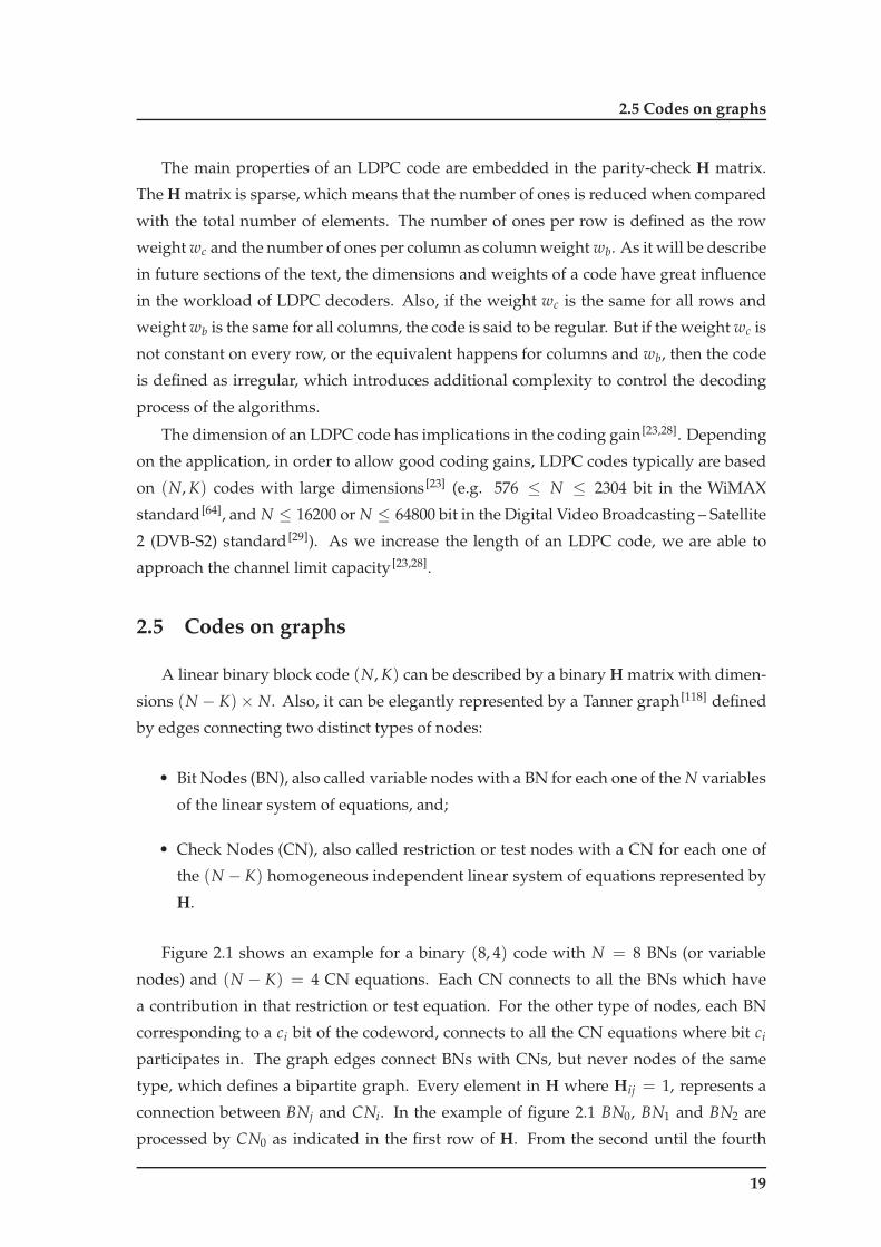
Figure 2.1 shows an example for a binary (8, 4) code with N = 8 BNs (or variable
nodes) and (N − K) = 4 CN equations. Each CN connects to all the BNs which have
a contribution in that restriction or test equation. For the other type of nodes, each BN
corresponding to a ci bit of the codeword, connects to all the CN equations where bit ci
participates in. The graph edges connect BNs with CNs, but never nodes of the same
type, which defines a bipartite graph. Every element in H where Hij = 1, represents a
connection between BNj and CNi. In the example of figure 2.1 BN0, BN1 and BN2 are
processed by CN0 as indicated in the first row of H. From the second until the fourth
19

2. Overview of Low-Density Parity-Check codes
CN0
CN1
CN2
CN3
00r20q
(8 Bit Nodes checked by 4 Check Node equations)
H =
BN0
CN0
BN1BN
2BN
3BN
4BN
5BN
6BN
7
1 1 1 0 0 0 0 0
0 0 0 1 1 1 0 0
1 0 0 1 0 0 1 0
0 1 0 0 1 0 0 1
CN1
CN2
CN3
BN0
BN1
BN2
BN3
BN4
BN5
BN6
BN7
c0+c
1+c
2=0
c3+c
4+c
5=0
c0+c
3+c
6=0
c1+c
4+c
7=0
Figure 2.1: A (8, 4) linear block code example: parity-check equations, the equivalent Hmatrix and corresponding Tanner graph [118] representation.
row, it can be seen that the subsequent BNs are processed by their neighboring CNs.
2.5.1 Belief propagation and iterative decoding
Graphical models, and in particular Tanner graphs as the one addressed in figure 2.1,
have often been proposed to perform approximate inference calculations [115,117]. They are
based on iterative intensive message-passing algorithms also known as belief propagation
(BP) which, under certain circumstances, can become computationally prohibitive. BP,
also known as the Sum-Product Algorithm (SPA)1, is an iterative algorithm [122] for the
computation of joint probabilities on graphs commonly used in information theory (e.g.
channel coding), artificial intelligence (AI) and computer vision (e.g. stereo vision) [19,117].
It has proved to be efficient and is used in numerous applications including LDPC codes [134],
Turbo codes [9,10], stereo vision applied to robotics [117], or in Bayesian networks such as
the QMR-DT (a decision-theoretic reformulation of the Quick Medical Reference (QMR))
model described in [77]).
1In the literature, the terms BP and SPA are commonly undistinguished. Both are used in this text withoutdifferentiation.
20

2.5 Codes on graphs
Encoder DecoderChannelc y cm
Figure 2.2: Illustration of channel coding for a communication system.
LDPC decoding: In this text we are interested in the BP algorithm applied to LDPC de-
coding. In particular, we exploit the Min-Sum Algorithm (MSA), one of the most efficient
simplification of the SPA, which are very demanding from a computational perspective.
The SPA applied to LDPC decoding operates with probabilities [46], exchanging informa-
tion and updating messages between neighbors over successive iterations.
Considering a codeword that we wish to transmit over a noisy channel, the theory of
graphs applied to error correcting codes has fostered codes to performances extremely
close of the Shannon limit [23]. In bipartite graphs, particularly in those with large dimen-
sions (e.g. N > 1000 bit), the certainty on a bit can be spread over neighboring bits of
a codeword allowing, in certain circumstances, in the presence of noise, to recover the
correct bits on the decoder side of the system. In a graph representing a linear block error
correcting code, reasoning algorithms exploit probabilistic relationships between nodes
imposed by parity-check conditions that allow inferring the most likely transmitted code-
word. The BP mentioned before allows to find the maximum a posteriori probability (APP)
of vertices in a graph [122].
Soft decoding: Propagating probabilities across nodes of the Tanner graph, rather than
just flipping bits [46] which is considered hard decoding, is defined as soft decoding. This
iterative procedure accumulates evidence imposed by parity-check equations that try to
infer the true value for each bit of the received word. Considering in figure 2.2 the original
unmodulated codeword c at the encoder’s output and the received word y at the input
of the decoder, we seek the codeword c ∈ C that maximizes the probability:
p(c|y, HcT = 0). (2.13)
However, this represents very intensive computation because all 2K codewords have to be
tested. An alternative that makes the decoder perform more localized processing consists
of testing only bit cn of all codewords and find a codeword that maximizes the probabil-
ity:
p(cn|y, all checks involving bit cn are satisfied). (2.14)
This represents the APP for that single bit, and only the parity-check equations that par-
ticipate in bit cn are satisfied. It defines one of two kinds of probabilities used in the
21

2. Overview of Low-Density Parity-Check codes
CN1
(i)00r
BN0
(i)10r
Edge 1
Edge 2
CN0
(i)01q
Figure 2.3: Detail of a check node update by the bit node connected to it as defined in theTanner graph for the example shown in figure 2.5. It represents the calculation of qnm(x)probabilities given by (2.16).
decoding algorithm [94] and can be denoted as:
qn(x) = p(cn = x|y, all checks involving bit cn are satisfied), x ∈ X. (2.15)
A variant from (2.15) isolates from this computation the parity-check m that participates
in bit n:
qnm(x) = p(cn = x|y, all checks, except check m, involving bit cn are satisfied), x ∈ X,
(2.16)
and is used to infer decisions on a decoded bit value. The computation of probabilities
qnm(x) are illustrated in figure 2.3, which represents the update of a q(i)nm message during
iteration i.
The second type of probabilities used in the decoding algorithm indicates the prob-
ability of parity-check m is satisfied, given only a single bit cn that participates in that
parity-check (and all the other observations associated with that parity-check), and it is
denoted as:
rmn(x) = p(Hm cT = 0, cn = x|y), x ∈ X, (2.17)
where the notation Hm cT = 0 represents the linear parity-check constraint m that satisfies
the codeword c. Probabilities rmn(x) are calculated according to the illustration shown
in figure 2.4, which represents the update of a r(i)mn message during iteration i. The com-
putation of probabilities qnm(x) and rmn(x), with x ∈ X, is performed iteratively only for
non-null elements of Hmn, with 0 < m < N − K − 1 and 0 < n < N − 1, i.e. across the
Tanner graph edges. The decoder computes probabilities about parity-checks (rmn(x))
which are then used to compute information about the bits (qnm(x)), on an iterative basis.
This propagation of evidence through the tree generated by the Tanner graph, depicted
in figure 2.5, allows to infer the correct codeword after all parity-checks are satisfied, or
abort after a certain number of iterations is reached.
22

2.5 Codes on graphs
CN1
(i-1)51q
(i-1)31q
BN4
BN5
BN3
(i-1)41q
Edge 1 Edge 3
Edge 2(i)
14r
Figure 2.4: Detail of a bit node update by the constraint check node connected to it asdefined in the Tanner graph for the example depicted in figure 2.5. It represents thecalculation of rmn(x) probabilities given by (2.17).
2.5.2 The Sum-Product algorithm
Given a (N, K) binary LDPC code, Binary Phase Shift Keying (BPSK) modulation is
assumed, which maps a codeword c = (c0, c1, c2, · · · , cn−1) into a sequence x = (x0, x1, x2,
· · · , xn−1), according to xi = (−1)ci . Then, x is transmitted over an additive white Gaus-
sian noise (AWGN) channel, producing a received sequence y = (y0, y1, y2, · · · , yn−1)
with yi = xi + ni, where ni represents AWGN with zero mean and variance σ2 = N0/2.
The SPA applied to LDPC decoding is illustrated in algorithm 2.1 and is mainly de-
scribed by two different horizontal and vertical intensive processing blocks defined, re-
spectively, by (2.18) to (2.19) and (2.20) to (2.21) [94]. The equations in (2.18) and (2.19)
calculate the message update from CNm to BNn, considering accesses to H in a row-
major basis – the horizontal processing – and indicate the probability of BNn being 0 or
1. For each iteration, r(i)mn values are updated according to (2.18) and (2.19), as defined by
the Tanner graph [79] illustrated in figure 2.5.
Similarly, the latter pair of equations (2.20) and (2.21) computes messages sent from
BNn to CNm, assuming accesses to H in a column-major basis – the vertical processing. In
this case, q(i)nm values are updated according to (2.20) and (2.21) and the edges connectivity
indicated by the Tanner graph.
Considering the message propagation from nodes CNm to BNn and vice-versa, the
set of bits that participate in check equation m, with bit n excluded, is represented by
N (m)\n and, similarly, the set of check equations in which bit n participates with check
m excluded isM(n)\m.
Finally, (2.22) and (2.23) compute the a posteriori pseudo-probabilities and in (2.24) the
hard decoding is performed at the end of an iteration. The iterative procedure is stopped
if the decoded word c verifies all parity-check equations of the code (HcT = 0), or if the
maximum number of iterations I is reached.
23

2. Overview of Low-Density Parity-Check codes
Check Node 0 updatingBit Nodes 0, 1 and 2
Check Node 1 updatingBit Nodes 3, 4 and 5
Check Node 2 updatingBit Nodes 0, 3 and 6
CN0
CN1
CN2
CN3
BN3
BN4
BN5
BN6
BN2
BN1
BN0
BN7
(i)00r
(i-1)10q
CN0
CN1
CN2
CN3
BN6
BN2
BN1
BN0
BN7
(i)14r
(i-1)31q
(i-1)51q
CN0
CN2
CN2
CN3
BN6
BN2
BN1
BN0
BN7
(i)26r
(i-1)32q
(i-1)02q
(i-1)00q
(i)01r
(i)02r
(i-1)41q
(i)13r
(i)15r
(i-1)62q
BN3
BN4
BN5
BN6
BN2
BN1
BN0
BN7
(i)23r
(i)20r
BN5
BN4
BN3
BN5
BN4
BN3
(i-1)20q
zoom area
CN1
(i-1)51q
(i-1)41q
BN4
BN5
BN3
(i-1)31q
Edge 1 Edge 3
Edge 2
zoomed area
(t)
Direction of processing
Figure 2.5: Tanner graph [118] expansion showing the iterative decoding procedure for thecode shown in figure 2.1.
24

2.5 Codes on graphs
Algorithm 2.1 Sum-Product Algorithm – SPA1: /* Initialization */
pn = 1
1+e2ynσ2
; EbN0
= N2Kσ2 ;
pn = p(yi = 1); q(0)mn(0) = 1− pn; q(0)mn(1) = pn;
2: while (HcT 6= 0 ∧ i < I) /* c-decoded word; I-Max. no. of iterations. */do
3: /* For all node pairs (BNn, CNm), corresponding to Hmn = 1 in the parity check matrix H of the code do:*/
4: /* Compute the message sent from CNm to BNn, that indicates the probability of BNn being 0 or 1: */
(Kernel 1 – Horizontal Processing)
r(i)mn (0) =
12+
12 ∏
n′∈N (m)\n
(
1− 2q(i−1)n′m (1)
)
(2.18)
r(i)mn (1) = 1− r(i)
mn (0) (2.19)
/* where N (m)\n represents BN’s connected to CNm excluding BNn. */
5: /* Compute message from BNn to CNm: */
(Kernel 2 – Vertical Processing)
q(i)nm (0) = knm (1− pn) ∏
m′∈M(n)\m
r(i)m′n (0) (2.20)
q(i)nm (1) = knm pn ∏
m′∈M(n)\m
r(i)m′n (1) (2.21)
/* where knm are chosen to ensure q(i)nm (0) + q(i)
nm (1) = 1, andM(n)\m is the set of CN’s connected toBNn excluding CNm. */
6: /* Compute the a posteriori pseudo-probabilities: */
Q(i)n (0) = kn (1− pn) ∏
m∈M(n)
r(i)mn (0) (2.22)
Q(i)n (1) = kn pn ∏
m∈M(n)
r(i)mn (1) (2.23)
/* where kn are chosen to guarantee Q(i)n (0) + Q(i)
n (1) = 1. */
7: /* Perform hard decoding: */∀n,
c(i)n =
{
1 ⇐ Q(i)n (1) > 0.5
0 ⇐ Q(i)n (1) < 0.5
(2.24)
8: end while
2.5.3 The Min-Sum algorithm
A logarithmic version of the well known SPA [46,83] defined as Logarithmic Sum-Product
Algorithm (LSPA) can be derived to achieve a less computationally demanding LDPC
25

2. Overview of Low-Density Parity-Check codes
decoding algorithm. Instead of the analysis of two complementary probabilities, this
simplification is based on the logarithm of their ratio, defined as the Log-likelihood
ratio (LLR). From a computational perspective the complexity of processing decreases as
it uses sum operations instead of multiplications, while subtractions replace divisions [63].
Log-likelihood ratio: Consider the complementary APP, p(cn = 0|y) and p(cn = 1|y)
which sum to 1. These two probabilities can be efficiently represented as a unique num-
ber by computing their ratio. Its logarithmic representation is given by:
LLR = log(p(cn = 0|y)p(cn = 1|y)
). (2.25)
The MSA [56] consists of a simplification of the LSPA [46,83] and is one of the most effi-
cient algorithms used to perform LDPC decoding [79]. Like the LSPA, the MSA is based
on the intensive belief propagation between nodes connected as indicated by the Tanner
graph edges (see example in figure 2.5), but only uses comparison and addition opera-
tions. Although its workload is lower than the one required by the SPA, it is still quite
significant. If the number of nodes is large (in the order of thousands) the MSA can still
demand very intensive processing.
The MSA is depicted in algorithm 2.2 [79]. Lpn designates the a priori LLR of BNn, de-
rived from the values received from the channel, and Lrmn is the message that is sent from
CNm to BNn, computed based on all received messages from BNs N (m)\n. Also, Lqnm
is the LLR of BNn, which is sent to CNm and calculated based on all messages received
from CNs M(n)\m and the channel information Lpn. For each node pair (BNn, CNm)
we initialize Lqnm with the probabilistic information received from the channel, and then
we proceed to the iterative body of the algorithm. Like the SPA, it is mainly described
by two horizontal and vertical intensive processing blocks, respectively defined by (2.26)
and (2.29). The former calculates the message updating procedure from each CNm to
BNn, considering accesses to H on a row basis. It indicates the likelihood of BNn being
0 or 1. The operations sign(.), min(.) (of any two given numbers), and abs(.) described
in (2.26), (2.27) and (2.28) represent a simplification of the computation defined in the
SPA, and can be performed quite efficiently both in hardware and software. The vertical
processing defined in kernel 2 and described in (2.29) computes messages sent from BNn
to CNm, assuming accesses to H on a column basis.
In (2.30) the a posteriori LLR are processed and stored into LQn, after which we per-
form the final hard decoding. Differently from the hard decoding decision performed for
the SPA in (2.24), here a decision on a bit value can be obtained simply by inspecting the
signal of LQn. The decision on c is described in (2.31) and it can be performed by sim-
ple and efficient hardware (and also software) operations, which represents an important
26

2.5 Codes on graphs
Algorithm 2.2 Min-Sum Algorithm – MSA1: /* Initialization */
Lpn =2yn
σ2 ;
Lq(0)nm = Lpn;
2: while (HcT 6= 0 ∧ i < I) /* c-decoded word; I-Max. no. of iterations. */do
3: /* For all node pairs (BNn, CNm), corresponding to Hmn = 1 in the parity check matrix H of the code do:*/
4: /* Compute the LLR of messages sent from CNm to BNn: */
(Kernel 1 – Horizontal Processing)
Lr(i)mn = ∏
n′∈N (m)\nαn′m min
n′∈N (m)\nβn′m, (2.26)
withαnm
∆= sign
(
Lq(i−1)nm
)
, (2.27)
andβnm
∆=
∣∣∣Lq(i−1)
nm
∣∣∣ . (2.28)
/* where N (m)\n represents BN’s connected to CNm excluding BNn. */
5: /* Compute the LLR of messages sent from BNn to CNm: */
(Kernel 2 – Vertical Processing)
Lq(i)nm = Lpn + ∑
m′∈M(n)\m
Lr(i)m′n. (2.29)
/* whereM(n)\m represents the set of CN’s connected to BNn excluding CNm. */
3. Finally, we compute the a posteriori LLRs:
LQn(i) = Lpn + ∑
m′∈M(n)
Lr(i)m′n. (2.30)
6: /* Perform hard decoding: */
c(i)n = −sign(LQ(i)
n ) (2.31)
7: end while
advantage for any architecture that performs intensive LDPC decoding.
Once again the iterative procedure is stopped if the decoded word c verifies all parity
check equations of the code (HcT = 0), or a predefined maximum number of iterations is
reached, in which case the processing can terminate without obtaining a valid codeword.
27
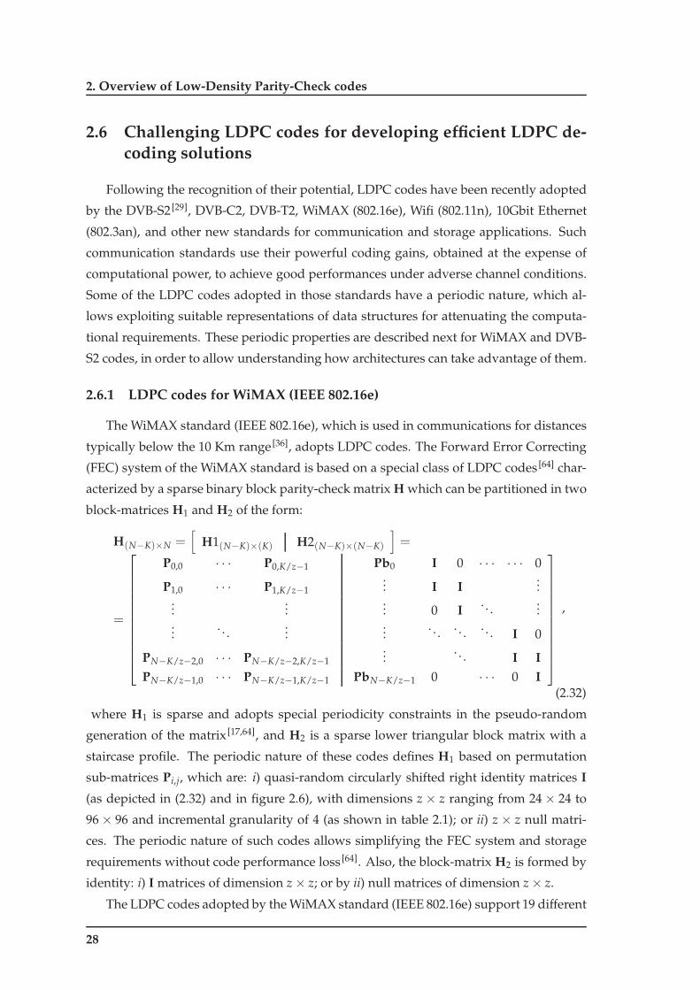
2. Overview of Low-Density Parity-Check codes
2.6 Challenging LDPC codes for developing efficient LDPC de-coding solutions
Following the recognition of their potential, LDPC codes have been recently adopted
by the DVB-S2 [29], DVB-C2, DVB-T2, WiMAX (802.16e), Wifi (802.11n), 10Gbit Ethernet
(802.3an), and other new standards for communication and storage applications. Such
communication standards use their powerful coding gains, obtained at the expense of
computational power, to achieve good performances under adverse channel conditions.
Some of the LDPC codes adopted in those standards have a periodic nature, which al-
lows exploiting suitable representations of data structures for attenuating the computa-
tional requirements. These periodic properties are described next for WiMAX and DVB-
S2 codes, in order to allow understanding how architectures can take advantage of them.
2.6.1 LDPC codes for WiMAX (IEEE 802.16e)
The WiMAX standard (IEEE 802.16e), which is used in communications for distances
typically below the 10 Km range [36], adopts LDPC codes. The Forward Error Correcting
(FEC) system of the WiMAX standard is based on a special class of LDPC codes [64] char-
acterized by a sparse binary block parity-check matrix H which can be partitioned in two
block-matrices H1 and H2 of the form:
H(N−K)×N =[
H1(N−K)×(K) H2(N−K)×(N−K)
]
=
=
P0,0 · · · P0,K/z−1 Pb0 I 0 · · · · · · 0
P1,0 · · · P1,K/z−1... I I
......
...... 0 I
. . ....
.... . .
......
. . . . . . . . . I 0
PN−K/z−2,0 · · · PN−K/z−2,K/z−1...
. . . I I
PN−K/z−1,0 · · · PN−K/z−1,K/z−1 PbN−K/z−1 0 · · · 0 I
,
(2.32)
where H1 is sparse and adopts special periodicity constraints in the pseudo-random
generation of the matrix [17,64], and H2 is a sparse lower triangular block matrix with a
staircase profile. The periodic nature of these codes defines H1 based on permutation
sub-matrices Pi,j, which are: i) quasi-random circularly shifted right identity matrices I
(as depicted in (2.32) and in figure 2.6), with dimensions z × z ranging from 24× 24 to
96× 96 and incremental granularity of 4 (as shown in table 2.1); or ii) z × z null matri-
ces. The periodic nature of such codes allows simplifying the FEC system and storage
requirements without code performance loss [64]. Also, the block-matrix H2 is formed by
identity: i) I matrices of dimension z× z; or by ii) null matrices of dimension z× z.
The LDPC codes adopted by the WiMAX standard (IEEE 802.16e) support 19 different
28

2.6 Challenging LDPC codes for developing efficient LDPC decoding solutions
H2H1
Check nodes
Bit nodes
z=96
z=96
(Parity-check bits)(Information bits)
Figure 2.6: Periodicity z× z = 96× 96 for an H matrix with N = 2304, rate = 1/2 and{3, 6} CNs per column.
Table 2.1: Properties of LDPC codes used in the WiMAX IEEE 802.16e standard [64].Code Codeword bits (N) z × z factor Information bits (K)
(rate) (rate) (rate) (rate)1/2 2/3 3/4 5/6
1 576 24 × 24 288 384 432 4802 672 28 × 28 336 448 504 5603 768 32 × 32 384 512 576 6404 864 36 × 36 432 576 648 7205 960 40 × 40 480 640 720 8006 1056 44 × 44 528 704 792 8807 1152 48 × 48 576 768 864 9608 1248 52 × 52 624 832 936 10409 1344 56 × 56 672 896 1008 1120
10 1440 60 × 60 720 960 1080 120011 1536 64 × 64 768 1024 1152 128012 1632 68 × 68 816 1088 1224 136013 1728 72 × 72 864 1152 1296 144014 1824 76 × 76 912 1216 1368 152015 1920 80 × 80 960 1280 1440 160016 2016 84 × 84 1008 1344 1512 168017 2112 88 × 88 1056 1408 1584 176018 2208 92 × 92 1104 1472 1656 184019 2304 96 × 96 1152 1536 1728 1920
29

2. Overview of Low-Density Parity-Check codes
codeword sizes with 4 distinct code rates and 6 different class codes (distinct distributions
of the number of BNs per column or CNs per row). They are depicted in table 2.1. Class
2/3A defines codes having {2, 3, 6} BNs per row and {10} CNs per column, while in
class 2/3B codes have {2, 3, 4} BNs and {10, 11} CNs. Also, class 3/4A has {2, 3, 4} BNs
and {14, 15} CNs, and class 3/4B has {2, 3, 6} BNs per row and {14, 15} CNs per column.
To illustrate the periodic nature introduced in the design of H, the matrix structure for
N = 2304 bit and rate = 1/2, is depicted in figure 2.6.
2.6.2 LDPC codes for DVB-S2
The FEC system of the recent DVB-S2 standard [29] incorporates a special class of
LDPC codes based on Irregular Repeat Accumulate (IRA) codes [30,67]. The parity-check
matrix H is of the form:
H(N−K)×N =[
A(N−K)×K B(N−K)×(N−K)
]
=
=
a0,0 · · · a0,K−1 1 0 · · · · · · · · · 0
a1,0 · · · a1,K−1 1 1 0...
...... 0 1 1
. . ....
.... . .
......
. . . . . . . . . 0...
aN−K−2,0 · · · aN−K−2,K−1...
. . . 1 1 0aN−K−1,0 · · · aN−K−1,K−1 0 · · · · · · 0 1 1
, (2.33)
where A is sparse and has periodic properties and B is a staircase lower triangular matrix.
The periodicity constraints put on the pseudo-random generation of A matrices allow a
significant reduction on the storage requirements without code performance loss. As-
sume that the N bits of a codeword are represented in the systematic form, divided in
information bits (IN) and parity-check bits (PN). The construction technique used to
generate the A matrix consists of splitting the IN nodes in disjoint groups of M = 360
consecutive 1’s. All the IN nodes of a group l should have the same weight wl and it
is only necessary to choose the CNm nodes that connect to the first IN of the group, in
order to specify the CNm nodes that connect to each one of the remaining (N − K− 1) IN
nodes. The connection choice for the first elements of group l is pseudo-random but it
guarantees that in the resulting LDPC code all the CNm nodes must connect to the same
number of IN nodes. Denoting by r1, r2, ..., rwl , the indices of the CNm nodes that con-
nect to the first IN of group l, the indices of the CNm nodes that connect to INi, with
0 < i < N − K− 1, of group l can be obtained by:
(r1 + i× q)mod(N − K), (r2 + i× q)mod(N − K), ..., (rwl + i× q)mod(N − K), (2.34)
with
q = (N − K)/M. (2.35)
30

2.6 Challenging LDPC codes for developing efficient LDPC decoding solutions
Table 2.2: Properties of LDPC codes2 used in the DVB-S2 standard [29] for the short framelength.
rate Codew. bits (N) Inf. bits (K) Col. weight (wb) Row weight (wc) # Edges
1/4 16200 4050 {3, 12} {4}* 486001/3 16200 5400 {3, 12} {5} 540002/5 16200 6480 {3, 12} {6} 583201/2 16200 8100 {3, 8} {6}* 486003/5 16200 9720 {3, 12} {11} 712802/3 16200 10800 {3, 13} {10} 540003/4 16200 12150 {3, 12} {12}* 486004/5 16200 12960 {3} {14}* 453605/6 16200 13500 {3, 13} {19}* 513008/9 16200 14400 {3, 4} {27} 48600
The factor M = 360 is constant for all codes used in the DVB-S2 standard. For each
code, A has groups of IN nodes with constant weights wc > 3, and also groups with
weights wc = 3. Matrix B has a lower triangle staircase profile as shown in (2.33). The
LDPC codes adopted by the DVB-S2 standard support two different frame lengths, one
for short frames (N = 16200 bit) and the other for normal frames (N = 64800 bit). The
short frame mode supports 10 distinct code rates as depicted in table 2.2, while the latter
supports 11 rates as shown in table 2.3. The column and row weights are also depicted
in tables 2.2 and 2.3 for all rates in the standard. For short frame lengths, all codes have
constant weight wc, with the exception of five of them2 as indicated in table 2.2, while
BNs have two types of weights wb, except for code with rate = 4/5 which has constant
weight wb = 3. For normal frame length codes, all CNs have a constant weight wc, while
BNs have two types of weights wb for each rate, as indicated in table 2.3.
Both tables show the number of edges for each code adopted in the DVB-S2 standard.
In each edge circulates a message that is used to update the corresponding node it con-
nects to. A closer inspection, for example, of code with rate = 3/5 for normal frames,
shows that the total number of edges of the Tanner graph is 285120. If we consider that
communications occur in both directions (from CNs to BNs, and then from BNs to CNs),
570240 > 512K messages are exchanged per iteration, which imposes huge computa-
tional demands (at several levels) for the development of LDPC decoders. In order to
perform efficiently these data communications and associated computations, the analy-
sis of LDPC decoding algorithms is performed in the next chapter, paving the way for
the analysis of programming models and architectures that suit such types of extremely
2The five short frame codes marked with the symbol * don’t have a constant weight per row wc, sincethey have been shortened has defined in the standard [29]. Consequently, they have rates which are an ap-proximation to those mentioned in this table, but not exactly the same.
31

2. Overview of Low-Density Parity-Check codes
Table 2.3: Properties of LDPC codes used in the DVB-S2 standard [29] for the normal framelength.
rate Codew. bits (N) Inf. bits (K) Col. weight (wb) Row weight (wc) # Edges
1/4 64800 16200 {3, 12} {4} 1944001/3 64800 21600 {3, 12} {5} 2160002/5 64800 25920 {3, 12} {6} 2332801/2 64800 32400 {3, 8} {7} 2268003/5 64800 38880 {3, 12} {11} 2851202/3 64800 43200 {3, 13} {10} 2160003/4 64800 48600 {3, 12} {14} 2268004/5 64800 51840 {3, 11} {18} 2332805/6 64800 54000 {3, 13} {22} 2376008/9 64800 57600 {3, 4} {27} 1944009/10 64800 58320 {3, 4} {30} 194400
demanding processing systems in the following chapters.
2.7 Summary
The properties of a particular family of linear block codes – LDPC codes –, based
on intensive belief propagation algorithms and their simplified variants, are introduced.
Although LDPC codes have been discovered almost half a century ago, due to huge com-
putational requirements only recently they have recaptured the attention of the scientific
community.
In this chapter it is given a brief introduction to belief propagation. The iterative
decoding representation based on bipartite or Tanner graphs of two main classes of al-
gorithms used in LDPC decoding is described, with particular focus given on the type of
processing required, and on the intensive nature of communications. Also, an overview
of the periodic nature of LDPC codes adopted in two important and recent standards
is introduced. In this overview, the mechanisms adopted for the generation of matrices
used in LDPC decoding are equally described.
In the next chapter, the complexity of these algorithms and corresponding computa-
tional requirements will be addressed, namely concerning the adoption of computational
models and parallelization approaches to accelerate this type of intensive processing.
32

"Computers in the future may weigh no more than 1.5 tons."
Popular Mechanics, 1949


3Computational analysis of LDPC
decoding
Contents3.1 Computational properties of LDPC decoding algorithms . . . . . . . . 36
3.1.1 Analysis of memory accesses and computational complexity . . . 36
3.1.2 Analysis of data precision in LDPC decoding . . . . . . . . . . . . 40
3.1.3 Analysis of data-dependencies and data-locality in LDPC decoding 41
3.2 Parallel processing . . . . . . . . . . . . . . . . . . . . . . . . . . . . . . . 44
3.2.1 Parallel computational approaches . . . . . . . . . . . . . . . . . . 44
3.2.2 Algorithm parallelization . . . . . . . . . . . . . . . . . . . . . . . 46
3.2.3 Evaluation metrics . . . . . . . . . . . . . . . . . . . . . . . . . . . 49
3.3 Parallel algorithms for LDPC decoding . . . . . . . . . . . . . . . . . . 50
3.3.1 Exploiting task and data parallelism for LDPC decoding . . . . . 50
3.3.2 Message-passing schedule for parallelizing LDPC decoding . . . 52
3.3.3 Memory access constraints . . . . . . . . . . . . . . . . . . . . . . 57
3.4 Analysis of the main features of parallel LDPC algorithms . . . . . . . 61
3.4.1 Memory-constrained scaling . . . . . . . . . . . . . . . . . . . . . 61
3.4.2 Scalability of parallel LDPC decoders . . . . . . . . . . . . . . . . 62
3.5 Summary . . . . . . . . . . . . . . . . . . . . . . . . . . . . . . . . . . . . . 63
35
3. Computational analysis of LDPC decoding
In this chapter we analyze the computational properties of Low-Density Parity-Check
(LDPC) code decoders introduced in chapter 2, and propose strategies to achieve efficient
processing. To obtain high throughputs as required by communication standards, LDPC
decoders can demand very intensive computation. A huge number of arithmetic opera-
tions and memory accesses per second is necessary to support high throughputs related
with multimedia/storage system requirements. These applications typically impose se-
vere constraints in the processing of video, audio, and data communications to provide
services in real-time within a targeted quality. Such demanding for real-time processing
imposes the analysis of computational properties of LDPC decoding and the exploitation
of parallelism. We study the dependencies that may prevent such achievement, analyze
task-parallelism, data-parallelism and also the memory access requirements for perform-
ing LDPC decoding in parallel. Finally, we address the importance of selecting a proper
message-passing schedule mechanism within the family of LDPC decoding algorithms,
when targeting parallel computing architectures. A discussion about the scalability of
LDPC decoders in parallel architectures concludes the chapter.
3.1 Computational properties of LDPC decoding algorithms
To reduce the high number of arithmetic operations and memory accesses required by
the Sum-Product Algorithm (SPA) and Min-Sum Algorithm (MSA) we exploit a simplifi-
cation based in the Forward-and-Backward optimization [63]. We also use the MSA with
λ-min= 2 [56], which is a simplification of the SPA in order to reduce even further the
number of operations. Like the SPA, the MSA is based on the belief propagation between
connected nodes, as defined by the Tanner graph edges (and shown in the example of
figure 2.5), but only uses comparison and addition operations. The workload produced
is still quite intensive, but lower than the one demanded by the SPA.
3.1.1 Analysis of memory accesses and computational complexity
The SPA applied to LDPC decoding is illustrated in algorithm 2.1 and is mainly de-
scribed by two different horizontal and vertical intensive processing blocks defined, re-
spectively, by the pair of equations (2.18), (2.19) and (2.20), (2.21). In (2.18) and (2.19)
the message updating from CNm to BNn is calculated, considering accesses to H in a
row-major basis – the horizontal processing – obtaining the r(i)mn values that indicate the
probability of BNn being 0 or 1. Similarly, the latter pair of equations (2.20) and (2.21)
computes messages sent from BNn to CNm, assuming accesses to H in a column-major
basis – the vertical processing. In this case, q(i)nm values are updated according to (2.20)
and (2.21), and the edges connectivity indicated by the Tanner graph.
36

3.1 Computational properties of LDPC decoding algorithms
Table 3.1: Number of arithmetic and memory access operations per iteration for the SPA.SPA - Horizontal Processing
Number of operations
Multiplications 2(wc − 1)wcMAdditions (wc + 1)wc MDivisions 0
Memory Accesses (wc − 1)wc M + 2wcM
SPA - Vertical ProcessingNumber of operations
Multiplications 2(wb + 1)wbNAdditions N + wbNDivisions wbN
Memory Accesses ((wb − 1)wb + 1)2N + 2wbN
Decoding complexity of the SPA: Assuming a H matrix with M = (N − K) CNs
(rows) and N BNs (columns), a mean row weight wc and a mean column weight wb,
with wc, wb ≥ 2, table 3.1 presents the computational complexity in terms of the number
of floating-point add, multiply and division operations required for both the horizon-
tal and vertical steps in the SPA LDPC decoding algorithm. The table also presents the
number of memory accesses required and it can be seen that for both cases the com-
plexity expressed as a function of wc and wb is quadratic. Depending on the size of the
codeword and channel conditions (Signal-to-Noise Ratio (SNR)), the minimal through-
put necessary for an LDPC decoder to accommodate an application’s requirements can
imply a substantial number of (arithmetic and memory access) operations per second,
which justifies the investigation of new parallelism strategies for LDPC decoding.
The decoding complexity can, however, be reduced by using the efficient Forward-
and-Backward algorithm [63] that minimizes the number of memory accesses and opera-
tions necessary to update (2.18) to (2.21) in algorithm 2.1. In table 3.2, the number of op-
erations required by the Forward-and-Backward algorithm adopted in this work shows
linear complexity (as a function of wc and wb). This represents a reduction in the number
of arithmetic operations, and an even more significant decrease in memory access oper-
ations, which contributes to increase the arithmetic intensity, here defined as the ratio of
arithmetic operations per memory access. This property (a higher arithmetic intensity)
suits multi-core architectures conveniently, which often have their performance limited
by memory accesses [82]. For a regular code with rate = 12 , where N = 2M, wc = 2wb and
wb ≥ 2, the arithmetic intensity αSPA for the SPA is:
αSPA =(3w2
c − wc)M + (2w2b + 4wb + 1)N
(w2c + wc)M + (2w2
b + 2)N≈ 2, (3.1)
37

3. Computational analysis of LDPC decoding
Table 3.2: Number of arithmetic and memory access operations per iteration for the opti-mized Forward-and-Backward algorithm [63].
Forward and Backward - Horizontal ProcessingNumber of operations
Multiplications (5wc − 6)MAdditions (4wc − 2)MDivisions 0
Memory Accesses 3wc M
Forward and Backward - Vertical ProcessingNumber of operations
Multiplications (6wb − 4)NAdditions 2wbNDivisions wbN
Memory Accesses (3wb + 1)N
while the arithmetic intensity αFBA for the optimized Forward-and-Backward algorithm
can be obtained by:
αFBA =(9wc − 8)M + (9wb − 4)N
3wcM + (3wb + 1)N≈ 3. (3.2)
Decoding complexity of the MSA: Table 3.3 presents the number of compare, abs (ab-
solute value calculations), min (the smallest of two given numbers), and xor (for signal
calculation) operations per iteration of the MSA algorithm. It also shows the number of
memory accesses per iteration necessary to update (2.26) to (2.29). They exhibit linear
complexity as a function of wc and wb. Here, the arithmetic intensity can be described by
(3.3) for a regular code with rate = 12 , where N = 2M, wc = 2wb and wb ≥ 2.
αMin−Sum =(4wc − 1)M + 2wbN2wc M + (2wb + 1)N
≈ 1.5. (3.3)
The value αMin−Sum shows that when applying the λ-min algorithm, memory accesses
should be optimized in order to maximize performance. Moreover, the type of opera-
tions is simpler than in the case of the SPA due to the optimized Forward-and-Backward
algorithm [63,134,136].
Figure 3.1 shows the number of arithmetic and logic operations (ALO) and memory
access operations (MAO) per iteration – the total is indicated in the figure as mega opera-
tions (MOP) – performed by the previously mentioned three LDPC decoding algorithms,
for two different situations: a) wc = 6 and wb = 3; and b) wc = 14 and wb = 6. LDPC
codes A to E have (N, K) equal to (504, 252), (1024, 512), (4896, 2448), (8000, 4000) and
(20000, 10000), respectively. It can be seen that for a code of medium to large dimensions
38

3.1 Computational properties of LDPC decoding algorithms
Table 3.3: Number of arithmetic and memory access operations per iteration for the opti-mized MSA.
Min-Sum - Horizontal ProcessingNumber of operations
Comparisons wc Mabs wc Mmin (wc − 1)Mxor wc M
Memory Accesses 2wcM
Min-Sum - Vertical ProcessingNumber of operations
Additions/Subtractions 2wbNMemory Accesses (2wb + 1)N
such as code D, a total of 3 MOP is required for the SPA – arithmetic and logic operations
(ALO) and memory accesses (MAO) – per iteration, using wc and wb as depicted in 3.1 b).
Considering code E and using a typical value of 10 iterations for the same algorithm, we
nearly achieve 80 MOP. The workload of intensive LDPC decoding algorithms grows lin-
early with the number of iterations. The number of iterations typically ranges from 5 to
A B C D E0
0.5
1
1.5
2
Num
ber
of o
pera
tions
(M
OP
)
A B C D E0
1
2
3
4
5
6
7
8
Num
ber
of o
pera
tions
(M
OP
)
ALO−SPAALO−FBAALO−MSAMAO−SPAMAO−FBAMAO−MSATotal−SPATotal−FBATotal−MSA
ALO−SPAALO−FBAALO−MSAMAO−SPAMAO−FBAMAO−MSATotal−SPATotal−FBATotal−MSA
a) b)
Figure 3.1: Mega operations (MOP) per iteration for 5 distinct H matrices (A to E), witha) wc = 6 and wb = 3; and b) wc = 14 and wb = 6.
20 (a pessimistic assumption) [81,88]. The number of operations necessary to decode 1000
codewords is depicted in figure 3.2 for the 3 algorithms mentioned before, each running
15 iterations. In this figure, the total number of operations is indicated as giga operations
(GOP).
39

3. Computational analysis of LDPC decoding
A B C D E0
5
10
15
20
25
30N
umbe
r of
ope
ratio
ns (
GO
P)
A B C D E0
20
40
60
80
100
120
Num
ber
of o
pera
tions
(G
OP
)
ALO−SPAALO−FBAALO−MSAMAO−SPAMAO−FBAMAO−MSATotal−SPATotal−FBATotal−MSA
ALO−SPAALO−FBAALO−MSAMAO−SPAMAO−FBAMAO−MSATotal−SPATotal−FBATotal−MSA
a) b)
Figure 3.2: Giga operations (GOP) for the parallel decoding of 1000 codewords running15 iterations each, for the same H matrices referred in figure 3.1, with a) wc = 6 andwb = 3; and b) wc = 14 and wb = 6.
3.1.2 Analysis of data precision in LDPC decoding
The average number of iterations naturally influences the decoding time. For a low
SNR the number of iterations necessary for a codeword to converge is greater than for
higher SNRs. Figure 3.3 shows that the average number of iterations in the LDPC decod-
ing process depends on the SNR (represented by Eb/N0) of data received at the input of
the decoder. As shown in the figure, if we decode for example 108 bits using the WiMAX
LDPC code (576, 288) [64], for a maximum number of iterations equal to 50 and an SNR
of 1 dB, we can observe that the average number of iterations nearly reaches its maxi-
mum (50 in this case). On the other hand, if the SNR rises to 4 dB, the average number of
iterations drops below 4. Depending on the adopted code, LDPC decoders can achieve
very good performances (low Bit Error Rate (BER)) even for low SNRs, at the expense of
computational power.
Solutions that dedicate more bits to represent data (messages) can compare favorably
in terms of the number of iterations needed for the algorithm to converge, when we look
at state-of-the-art Application Specific Integrated Circuits (ASIC) LDPC decoders in the
literature [17,81,108,111] that use low precision architectures to represent data (e.g. 5 to 6-
bits). An additional advantage is observed in the BER curves for typical ASIC solutions.
A minimal data precision representation is fundamental in ASIC solutions in order to
achieve acceptable die area and power consumption. Figure 3.4 shows the BER curves
obtained for two different codes used in the WiMAX standard [64], namely (576,288) and
(1248,624) with either 6 or 8-bit precision. A MSA implementation, based on an 8-bit data
40

3.1 Computational properties of LDPC decoding algorithms
1 1.5 2 2.5 3 3.5 40
5
10
15
20
25
30
35
40
45
50
Eb/N
0 (dB)
Ave
rage
Num
ber
of It
erat
ions
6−bit, (576, 288)8−bit, (576, 288)6−bit, (1248, 624)8−bit, (1248, 624)
Figure 3.3: Average number of iterations per SNR, comparing 8-bit and 6-bit data preci-sion representations for WiMAX LDPC codes (576,288) and (1248,624) [64] running a max-imum of 50 iterations.
precision solution, achieves improved BER compared with ASIC solutions [17,81,108,111].
The programmable solutions proposed in this thesis and described later in future sec-
tions of the text, use either 32-bit floating-point single precision, or 8-bit integer precision
to represent data, which helps to improve the BER performance.
3.1.3 Analysis of data-dependencies and data-locality in LDPC decoding
The wcM messages involved per iteration in the horizontal step and the wbN mes-
sages required per iteration for the vertical step, are depicted in the two columns of ta-
ble 3.4, for the Tanner graph example shown in figure 2.5. The Fh(.) and Fv(.) functions
represent, respectively, the horizontal and vertical kernels described in algorithms 2.1
(for the SPA) and 2.2 (for the MSA), while miZ0→W0
denotes a message m passed from
node Z0 to node W0 during iteration i. In the vertical kernel, p0 represents the channel
information associated to BN0 and p7 the channel information for BN7.
Data-dependencies: The operations referred before can be parallelized by adopting a
suitable message-passing schedule that supports the updating corresponding to different
vertices or/and different messages, simultaneously, in distinct parts of the Tanner graph.
The main data-dependency constraints arise from the fact that all messages used in the
calculation of a new message in any iteration were obtained during the previous iteration.
41
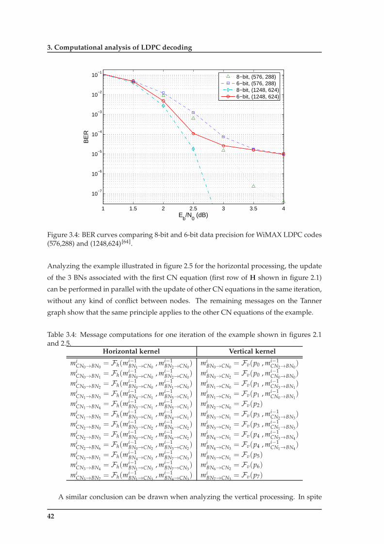
3. Computational analysis of LDPC decoding
1 1.5 2 2.5 3 3.5 4
10−7
10−6
10−5
10−4
10−3
10−2
10−1
Eb/N
0 (dB)
BE
R
8−bit, (576, 288)6−bit, (576, 288)8−bit, (1248, 624)6−bit, (1248, 624)
Figure 3.4: BER curves comparing 8-bit and 6-bit data precision for WiMAX LDPC codes(576,288) and (1248,624) [64].
Analyzing the example illustrated in figure 2.5 for the horizontal processing, the update
of the 3 BNs associated with the first CN equation (first row of H shown in figure 2.1)
can be performed in parallel with the update of other CN equations in the same iteration,
without any kind of conflict between nodes. The remaining messages on the Tanner
graph show that the same principle applies to the other CN equations of the example.
Table 3.4: Message computations for one iteration of the example shown in figures 2.1and 2.5.
Horizontal kernel Vertical kernel
miCN0→BN0
= Fh(mi−1BN1→CN0
, mi−1BN2→CN0
) miBN0→CN0
= Fv(p0 , mi−1CN2→BN0
)
miCN0→BN1
= Fh(mi−1BN0→CN0
, mi−1BN2→CN0
) miBN0→CN2
= Fv(p0 , mi−1CN0→BN0
)
miCN0→BN2
= Fh(mi−1BN0→CN0
, mi−1BN1→CN0
) miBN1→CN0
= Fv(p1 , mi−1CN3→BN1
)
miCN1→BN3
= Fh(mi−1BN4→CN1
, mi−1BN5→CN1
) miBN1→CN3
= Fv(p1 , mi−1CN0→BN1
)
miCN1→BN4
= Fh(mi−1BN3→CN1
, mi−1BN5→CN1
) miBN2→CN0
= Fv(p2)
miCN1→BN5
= Fh(mi−1BN3→CN1
, mi−1BN4→CN1
) miBN3→CN1
= Fv(p3 , mi−1CN2→BN3
)
miCN2→BN0
= Fh(mi−1BN3→CN2
, mi−1BN6→CN2
) miBN3→CN2
= Fv(p3 , mi−1CN1→BN3
)
miCN2→BN3
= Fh(mi−1BN0→CN2
, mi−1BN6→CN2
) miBN4→CN1
= Fv(p4 , mi−1CN3→BN4
)
miCN2→BN6
= Fh(mi−1BN0→CN2
, mi−1BN3→CN2
) miBN4→CN3
= Fv(p4 , mi−1CN1→BN4
)
miCN3→BN1
= Fh(mi−1BN4→CN3
, mi−1BN7→CN3
) miBN5→CN1
= Fv(p5)
miCN3→BN4
= Fh(mi−1BN1→CN3
, mi−1BN7→CN3
) miBN6→CN2
= Fv(p6)
miCN3→BN7
= Fh(mi−1BN1→CN3
, mi−1BN4→CN3
) miBN7→CN3
= Fv(p7)
A similar conclusion can be drawn when analyzing the vertical processing. In spite
42
3.1 Computational properties of LDPC decoding algorithms
of the irregular memory access pattern, in this case too it is possible to parallelize the
processing of the wbN new messages, as it is the case of miBN0→CN0
and miBN0→CN2
, that
exemplify the update of the two messages associated to BN0 (first column of H shown in
figure 2.1) and that can be performed in parallel with other messages.
Exploiting spatial locality: To permit the simultaneous update of messages, code and
data structures that allow exposing parallel properties of the algorithm for data read/write
operations should be considered. To efficiently exploit spatial locality it is also important
to consider the characteristics of the computational systems architecture. If this is not
the case, the impact of memory accesses may rise and, depending on the level of dis-
arrangement, have a significant weight in the processing efficiency. For example, the
memory hierarchy which typically has larger but slower memories as we move away
from the processor, may lead to poor speedups if the locality is not properly exploited
(e.g. caches).
In the context of LDPC decoding we group blocks of data associated to CNs and
BNs, with sizes that depend on the length of the code and the architecture being used. By
varying the granularity of data blocks, different results can be obtained [32,39], and a trade-
off between time spent performing communications and data size must be pursued in
order to achieve optimal results. Another aspect equally important for exploiting locality
consists of placing each one of these groups of data located together in memory. Runtime
data realignment techniques were developed [34] to tackle the problem that sometimes
arises from such procedure, due to the fact that data cannot be aligned at compile time.
They will be described in future sections of the text, for both horizontal and vertical
processing steps.
Exploiting temporal locality: Another aspect that assumes great importance for achiev-
ing efficient LDPC decoding is the proper exploitation of temporal locality. Temporal lo-
cality exists when a certain computation accesses the same group of data several times in
a short period of time. To exploit temporal locality in parallel systems, the computation
that accesses the same data should be assigned to the same processing unit. The main
goal here is to organize the processing so that those accesses to the same group of data
can be scheduled to execute close in time one to another. To achieve this, the program-
mer needs to organize the algorithm so that working sets are kept small enough to map
well on the sizes of the different levels of memory hierarchy, but not too small to cause
inefficiency.
The kernels developed for LDPC decoding in this thesis are structured to process
groups of BNs associated to the same CN for the horizontal processing. In the vertical
43
3. Computational analysis of LDPC decoding
processing, groups of CNs associated to the same BN can also be processed by the same
kernel. The advantage obtained here is clear: inside each kernel, common accesses to
data are repeated in very short periods of time for these groups of BNs and CNs, which
serves the purpose of special memory structures dedicated to exploit this property (e.g.
cache memory).
Either exploiting spatial or temporal locality, the message-passing schedule mecha-
nism assumes high importance regarding to data-dependencies, as it will be mentioned
later in section 3.3.2.
3.2 Parallel processing
The influence of parallel computing approaches and models in the performance of a
parallel application can be analyzed from different perspectives.
3.2.1 Parallel computational approaches
Although several sub-categories of parallel computational approaches can be consid-
ered, they mainly belong to one of two classes: task parallelism and data parallelism.
More detailed sub-classes of parallel computational approaches and models can be iden-
tified to target actual parallel systems.
Task parallelism: A task defines the smallest unit of concurrency that a program can
exploit. In parallel architectures, the granularity adopted when determining the size
of tasks (i.e. the number of instructions) should preferably use fine-grained or smaller
tasks, in order to stimulate workload balancing. On the other hand, it shouldn’t be too
small because in that case interprocessor communications and management overheads
would relatively rise, introducing penalties that may have a negative impact on the per-
formance.
Some parallel computing machines have a Multiple Instruction Multiple Data (MIMD)
stream architecture, where at any given instant, multiple processors can be executing, in-
dependently and asynchronously, different tasks or instructions on different blocks of
data.
Data parallelism: A simple way of exploiting algorithmic intrinsic parallelism consists
in using Single Instruction Multiple Data (SIMD), where programming resembles more
the serial programming style but the same instruction is applied to a collection of data,
all in parallel and at the same time. This model is usually supported on the SIMD stream
type of architectures, where several data elements can be kept and operated in parallel,
44

3.2 Parallel processing
namely inside special registers (SIMD within-a-register (SWAR), typically ranging from
128-bit to a 512-bit width).
In vector processing approaches, SIMD parallelism is used for processing regular data
structures. Stream processing is another example of data parallel programming where
kernels are applied in parallel rather than single instructions to a collection of data. The
input streaming data is gathered before processing, and results are scattered after finish-
ing it. A kernel can have many instructions and perform a large number of operations
per memory access. As the evolution of processing speed has been much superior than
the increase of memory bandwidth, the stream programming model suits better modern
multi-core architectures.
With Single Program Multiple Data (SPMD) parallelism, the kernels additionally sup-
port flow control. With the introduction of branches, the kernels can execute different
operations depending on conditions defined in run-time and still be efficient, as long
as workload balancing is properly considered. In this model, multiple threads are al-
lowed, however they can be executed as different sequential operations belonging to the
same program. For example, modern Graphics Processing Units (GPU), namely those
from NVIDIA which are conveniently supported by the recent Compute Unified Device
Architecture (CUDA) [97], adopted the SPMD computational model.
Shared memory versus distributed memory: In a parallel system, it is fundamental
to establish mechanisms that allow processors to communicate in order to cooperatively
complete a task (or set of tasks). Mainly two distinct memory models can be adopted in
parallel computing models and machines: shared memory and distributed memory1.
In a shared memory model, memory can be shared by all processors or, at least, dis-
tinct groups of processors can access common banks of memory. For example, with hi-
erarchical shared memory, faster memory can be accessed and shared inside subsets of
processors, while slower global memory is accessible to all processors. Furthermore, by
sharing memory within a limited number of processors (the dimension of the group of
processors is architecture dependent), we also decrease the potential for access conflicts.
Moreover, modern architectures support automatic mechanisms for efficient data trans-
fers between distinct levels of memory hierarchy (e.g. cache memory, or some compilers
ability to automatically place data in fast local/shared memory). However, this model
introduces an extra level of complexity necessary to guarantee data integrity.
On the opposite side we have architectures that only support distributed memory
models. In this case, each processor only has direct access to its own local memory.
1Although distributed shared memory systems exist with Non-Uniform Memory Architecture (NUMA),they will not be addressed under the context of this work.
45

3. Computational analysis of LDPC decoding
Different processors communicate with each other over high bandwidth networks us-
ing efficient mechanisms such as, for example, Direct Memory Access (DMA) that can
overlap data transfers with computation. Architectures based on the distributed mem-
ory model are scalable and easier to construct, but harder to program/debug than those
based on shared memory models. On a distributed memory model, inter-processor com-
munications have to be efficiently managed in order to allow a task (or set of tasks) to be
computed cooperatively by multiple processors.
As we will see in chapter 5, GPUs consist of parallel computing machines based on
shared memory models, where groups of processing units share common fast memory
blocks. The Cell Broadband Engine (Cell/B.E.) is an example of a distributed memory
architecture exploited in this thesis. A few standards already exist and can be used
to program parallel machines based on the different memory models. OpenMP [21], or
CUDA [97] are usually adopted to program general-purpose multi-core systems and GPUs,
which have shared memory architectures. They are based on a set of compiler directives,
library functions, or environment variables for developing parallel programs. On the
distributed model we can use the Message Passing Interface (MPI). Typically, a set of
library functions are provided, compliant with the MPI, that programmers can use to
communicate between processors.
In future versions-to-come of current parallel architectures, the number of processors
will expectedly rise. Assuming a shared memory architecture, a limit will arrive where
the bus occupancy and data collisions will have a significant impact on the global pro-
cessing time, causing performance to degrade. For this reason, usually this type of archi-
tecture has poor scalability when compared with distributed architectures, where each
processor can perform non-conflicting independent accesses to its own memory space.
However, we should be aware that to obtain short execution times in distributed systems,
we must have efficient schedulers and inter-processor communication mechanisms.
3.2.2 Algorithm parallelization
The job of translating a sequential algorithm into an efficient parallel version of its
own aims at the increase of performance and can be hard depending on the peculiar-
ities of the algorithm and restrictions imposed by the architecture. In many cases, the
best sequential algorithm indicated to solve a problem is not the best candidate for par-
allelization and a significantly different algorithm may be required [25].
Developing a good parallel algorithm involves identifying the amount of workload
that can be parallelized, creating appropriate parallel structures to represent data, decid-
ing how to distribute work and data among the several processing elements, as well as
managing the fundamental data accesses and data transfers maintaining data coherence,
46

3.2 Parallel processing
Table 3.5: Steps in the parallelization process and their goals [25].Step Architecture Dependent? Major Performance Goals
Decomposition Mostly no Expose enough concurrency
Assignment Mostly no Balance workload
Reduce communication volume
Orchestration Yes Reduce non inherent
communication via data locality
Reduce communication and
synchronization as seen by
the processor
Reduce serialization as shared
resources
Schedule tasks to satisfy
dependencies early
Mapping Yes Put related processes on the
same processor if necessary
Exploit locality in network topology
by controlling communications and synchronization. Another important aspect we have
to deal with is understanding the trade-offs between hardware and software. Not only
the architecture influences the performance of the algorithm and programming decisions,
but also programming decisions have an impact on the run-time characteristics of the al-
gorithm over an architecture. The following steps can be considered for designing and
implementing efficient parallel algorithms:
• decomposition of both computation into tasks and data into structures suitable for
parallel accesses;
• assignment of tasks to processes or threads2;
• orchestration of data (scheduling, transfers, accesses, communications and syn-
chronizations) among processes/threads;
• mapping processes/threads to processing units.
Table 3.5 illustrates the architecture dependencies and how these steps in the paral-
lelization procedure can influence the major performance goals. This procedure is per-
formed both by the programmer and by software tools/compilers/libraries designed to
support the architectures.
2Typically, processes contain their own state information and represent independent execution units.
47

3. Computational analysis of LDPC decoding
Algorithm structure
Supporting structures
Implementation mechanisms
Message-passing
schedulingData sharing
Group tasks
Order tasks
Data decomposition
Task decomposition
Decomposition
Dependency analysis
Finding concurrency
Design evaluation
Figure 3.5: Finding concurrency design space adapted from [25] to incorporate scheduling.
Decomposition: Decomposition can be understood as splitting the computation into
different tasks in order to expose concurrency. The order messages are passed (message-
passing scheduling) between adjacent nodes of the graph has a significant impact on the
decisions of breaking up the computation into blocks of tasks. Also, data can be split,
concatenated or reordered into new collections of data to suit concurrency. Figure 3.5
shows that the analysis of data-dependencies influences (task and data) decomposition.
Assignment: Deciding which tasks are distributed over which threads is accomplished
on the assignment step. The primary objective of assignment is to balance the workload
and minimize inter-process communication. The assignment can be statically predeter-
mined in the beginning of computation or dynamically reallocated during run-time. To-
gether, decomposition and assignment define the partitioning of the algorithm and usu-
ally they are the steps that less depend on the architecture.
Orchestration: In order to best orchestrate the run-time behavior of the algorithm, we
must understand the architecture and programming model in detail. This important step
Each process uses its own program counter, address space, and only interacts with other processes via inter-process communication mechanisms (which are usually managed by the operating system). Processes canbe defined as architectural constructs, while threads can be more adequately considered coding constructs.A single process might contain multiple threads, and all threads inside the process can communicate directlywith each other because they share common resources (e.g. memory space). Under the context of this text,although their differences remain clear, from now on the term thread will be used because it addresses moreappropriately the properties (at both algorithmic and architectural levels) of this work.
48

3.2 Parallel processing
uses all the available mechanisms to allow tasks inside threads accessing data, transfer-
ring it by communicating with other threads, or even synchronizing with one another.
Also, the orchestration can define the organization of data structures, the optimal size of
block data transfers between threads (enough to avoid starvation on the computation),
or the temporal scheduling of a task to minimize the impact of communication time in
the overall processing time.
Mapping: This last step maps threads into processors and naturally depends on the
architecture. The program can control this process, or the operating system may do it dy-
namically in its turn, not allowing control over the mapping procedure usually to achieve
effective aggregate resource sharing. Ideally, related threads should be mapped into the
same processor to allow fast data communication and synchronization. Mapping and or-
chestration are tightly coupled, so many times these parallelization steps are performed
together, to improve processing efficiency.
3.2.3 Evaluation metrics
The main goal of parallelizing an algorithm aims at an increase in performance, here
defined as speedup which compares the performance of sequential and parallel versions
of the algorithm. Although the number of cores (P) naturally influences speedup, typi-
cally the global increase in performance does not vary linearly with the number of cores.
The speedup is a metric to evaluate the level of success achieved with the parallelization
of an algorithm on an architecture with P processors, by comparing with a sequential
version of its own [25]:
Speedupalgorithm(P) =Sequential Time
Maximum Time on Any Processor. (3.4)
In (3.4) the term Time represents time spent performing the task, including computa-
tion, memory accesses, and data communications with the system’s main memory as
well. It gives a more approximate value of the real speedup achieved, by including the
limitations of the architecture (bandwidth, concurrency accessing global memory, data
collisions, multi-pipeline influences, etc.). Another usual metric for assessing the success
of parallelization on P cores is defined by efficiency (E f ), which normalizes the speedup
by the number of cores:
E f =Sequential Time
P×Maximum Time on Any Processor× 100% . (3.5)
49

3. Computational analysis of LDPC decoding
3.3 Parallel algorithms for LDPC decoding
In this section we apply the parallel computational models and the parallelization
approaches for LDPC decoding. It is also discussed the influence that the different types
of message-passing schedules can have in the performance of the parallel algorithms
used in LDPC decoding.
3.3.1 Exploiting task and data parallelism for LDPC decoding
Task parallelism in LDPCs: In the context of LDPC decoding, the smallest task that can
be defined should be responsible for updating a single edge of the Tanner graph. This ap-
proach would be efficient if the number of processors were large, and if memory accesses
did not impose restrictions. Different approaches can be more efficient, for example by
completely assigning a node of the Tanner graph to a task. In this case, depending on the
message-passing scheduling, redundant memory accesses and extra computation can be
saved [134,136], increasing performance.
Definition 3.1. Intra-codeword parallelism denotes the simultaneous processing of differ-
ent nodes of the Tanner graph within the same codeword, by different tasks or processing
units.
The concept associated to Definition 3.1 is illustrated in figure 3.6. It shows how
intra-codeword parallelism can be exploited to achieve LDPC decoding for the example
described in figure 2.1. It is based on the fact that the Tanner graph can be partitioned into
distinct subsets. Each one of those subsets can then be processed by a different task or
processing unit, in parallel, where tasks t0 to t3 are used to describe parallelism applied to
the horizontal kernel of algorithms 2.1 or 2.2, and tasks t0 to t7 represent the parallelism
applied to the vertical kernel.
Data parallelism in LDPCs: Data parallelism can be applied to exploit multi-codeword
LDPC decoding, as defined as follows:
Definition 3.2. Multi-codeword parallelism denotes the simultaneous decoding of different
codewords using distinct processing units, sharing the same Tanner graph information.
To exploit data parallelism in the context of LDPC decoding, the SIMD and SPMD ap-
proaches can be used. SIMD can be used directly for multi-codeword LDPC decoding [36],
where multiple codewords are decoded simultaneously according to Definition 3.2. Multi-
codeword decoding exploits the fact that the Tanner graph is common to all codewords
under simultaneous decoding. This allows to apply the same instruction to different data.
50
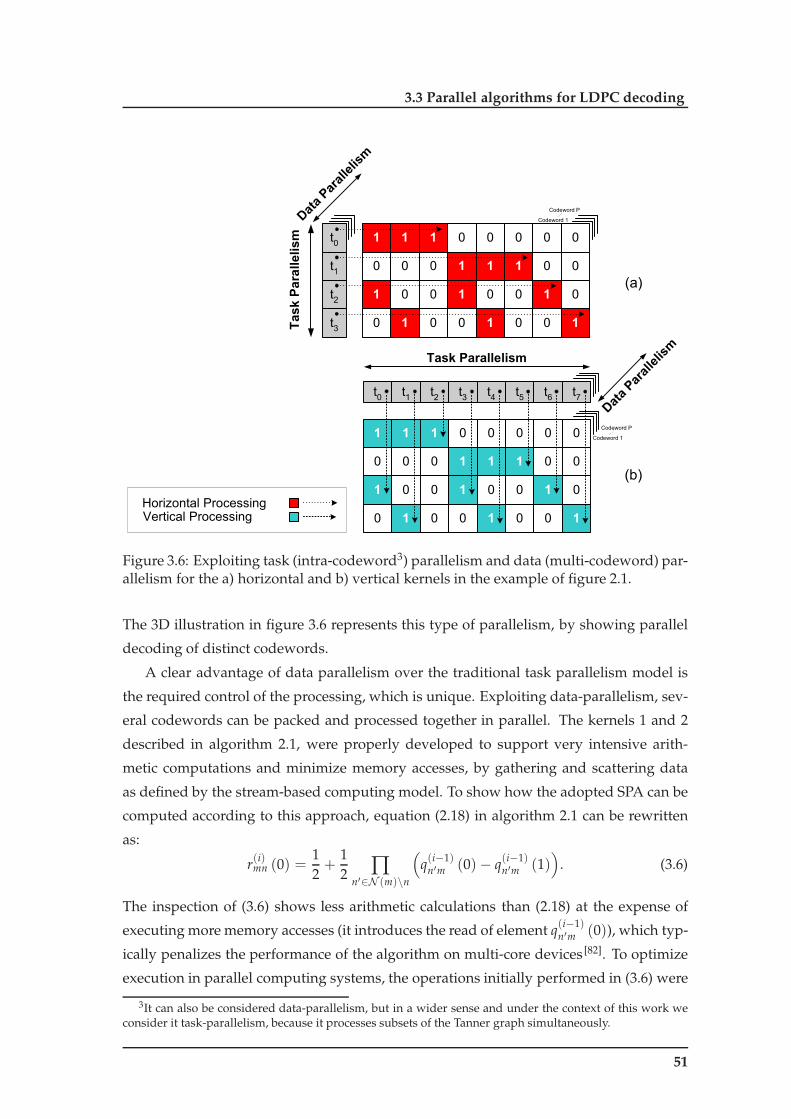
3.3 Parallel algorithms for LDPC decoding
1 1 1 0 0 0 0 0
0 0 0 1 1 1 0 0
1 0 0 1 0 0 1 0
0 1 0 0 1 0 0 1
t0
t1
t2
t3
t4
t5
t6
t7
1 1 1 0 0 0 0 0
0 0 0 1 1 1 0 0
1 0 0 1 0 0 1 0
0 1 0 0 1 0 0 1
t0
t1
t2
t3
Task Parallelism
Task Parallelism
Horizontal ProcessingVertical Processing
(a)
Codeword 1
Codeword P
Codeword 1
Codeword P
(b)
Data Parallelism
Data Parallelism
Figure 3.6: Exploiting task (intra-codeword3) parallelism and data (multi-codeword) par-allelism for the a) horizontal and b) vertical kernels in the example of figure 2.1.
The 3D illustration in figure 3.6 represents this type of parallelism, by showing parallel
decoding of distinct codewords.
A clear advantage of data parallelism over the traditional task parallelism model is
the required control of the processing, which is unique. Exploiting data-parallelism, sev-
eral codewords can be packed and processed together in parallel. The kernels 1 and 2
described in algorithm 2.1, were properly developed to support very intensive arith-
metic computations and minimize memory accesses, by gathering and scattering data
as defined by the stream-based computing model. To show how the adopted SPA can be
computed according to this approach, equation (2.18) in algorithm 2.1 can be rewritten
as:
r(i)mn (0) =12+
12 ∏
n′∈N (m)\n
(
q(i−1)n′m (0)− q(i−1)
n′m (1))
. (3.6)
The inspection of (3.6) shows less arithmetic calculations than (2.18) at the expense of
executing more memory accesses (it introduces the read of element q(i−1)n′m (0)), which typ-
ically penalizes the performance of the algorithm on multi-core devices [82]. To optimize
execution in parallel computing systems, the operations initially performed in (3.6) were
3It can also be considered data-parallelism, but in a wider sense and under the context of this work weconsider it task-parallelism, because it processes subsets of the Tanner graph simultaneously.
51

3. Computational analysis of LDPC decoding
mathematically manipulated and are preferably represented as indicated in (2.18), in or-
der to maximize the use of arithmetic operations regarding the number of memory ac-
cesses.
When developing code for an architecture that supports the SPMD computing model,
a programmer should concentrate efforts to use the same program and to minimize test
conditions. Sometimes, redesigning the algorithm may be necessary to eliminate unnec-
essary branches, which allows the hardware scheduler (i.e. task scheduler) to adopt a
more balanced workload distribution among processors. Although under certain condi-
tions the scheduler’s behavior can be very efficient, as it will be discussed later on the
text, the nature of LDPC decoders implies that each node establishes communications
with other nodes. To minimize the effect of overheads introduced by redundant commu-
nications and to allow the efficient Forward-and-Backward recursion [63] to be adopted,
the size of a task should not be set too small. For LDPC decoders under this model the
most efficient approach experimented under this thesis computes one complete set of
nodes per task. Typically, this set is composed by all the BNs associated to a CN for
horizontal processing, or by all CNs associated to a BN for vertical processing.
3.3.2 Message-passing schedule for parallelizing LDPC decoding
Chapter 2 shows that LDPC decoding algorithms are based on iterative procedures
with heavy computation and data communications associated to intensive message pass-
ing between adjacent nodes of the Tanner graph. For each type of node and iteration, the
update can be performed serially (one node at a time) or in parallel (several nodes si-
multaneously), that the output messages at the end of an iteration will be the same. The
order in which messages are propagated in the graph is relevant due to implications in
the efficiency of computation and on speed of convergence, influencing the overall per-
formance and coding gain of the algorithm [109]. The order of propagation can be defined
by the message-passing schedule mechanism.
Although in ideal cycle-free codes the message-passing schedule mechanism has no
influence on the convergence of the algorithm, in practice cycle-free codes are hard to
achieve and high-girth codes are acceptable and used in most applications. Thus, for
implementation purposes on parallel architectures, the adopted message-passing sched-
ule procedure is fundamental to achieve efficiency. We adopted fixed message-passing
schedule approaches as they allow fair trade-offs between hardware and algorithmic
costs.
Flooding schedule: In LDPC decoding algorithms, the complete processing of one it-
eration is divided in two different kernels, being one responsible for updating all the
52

3.3 Parallel algorithms for LDPC decoding
Step 1
Step 2
Step 3
Parallel update of all
the BNs in the Tanner
graph
Parallel update of all
the CNs in the Tanner
graph
Parallel update of all
the BNs in the Tanner
graph
Figure 3.7: Flooding schedule approach.
BNs and the other for updating the CNs in the Tanner graph. Figure 3.7 shows that the
flooding approach operates over this structure in parallel, simultaneously updating all
the BNs first, and then CNs after. For each type of node, the number of nodes being
simultaneously updated does not change the output results or the coding gain of the
algorithm.
Horizontal schedule: Figure 3.8 depicts an organization of processing that updates
each CN at a time. Each CNm processor collects data from the BNs connected to it, that
were either produced in the previous iteration, or in the present one by CNm′ proces-
sors, with m′ < m, that already updated their corresponding BNs. This latter approach
that uses data already updated in the current iteration, accelerates the convergence of the
algorithm as proposed in [86,109,131].
Algorithm 3.1 Algorithm for the horizontal schedule (sequential).1: /* Initializes data structures by reading a binary M× N matrix H */2: for all CNm (rows in Hmn) : do3: CNm ← BNn; /* BNn updates CNm... */4: for all BNn (columns in Hmn) : do5: if Hmn == 1 then6: /* CNm updates BNn, for all n ∈ N (m) previously updated by CNm′ , m′ < m */7: BNn ← CNm;8: end if9: end for
10: end for
Horizontal block schedule: To accelerate the previous type of serial processing, some
authors have proposed to simultaneously process blocks of P CN processors in parallel.
53

3. Computational analysis of LDPC decoding
Step 1
Step 2
Step 3
Update of checknode CN
0
Step 4
Update of bit nodesBN
nn N(0)
Update of checknode CN
1
Update of bit nodesBN
nn N(1)
Step 5
Step 6
Update of checknode CN
2
Update of bit nodesBN
nn N(2)
Step 7
Step 8
Update of checknode CN
3
Update of bit nodesBN
nn N(3)
Figure 3.8: Horizontal schedule approach.
The message-passing schedule inside each of these blocks can be considered flooding for
the P nodes under parallel processing. Figure 3.9 shows the update of P = 2 CNs in
parallel, and then the processing of all the BNs connected to them also in parallel. The
sequential approach depicted in figure 3.8 is presented in algorithm 3.1. As mentioned
before, to perform the updating procedure each CNm collects data from all connected BNn
that might have been already updated in the same iteration, allowing faster convergence
of the algorithm. The main disadvantage lies in processing sequentiality imposed by
such approach. The horizontal block schedule depicted in figure 3.9 is expanded into
algorithm 3.2, where groups of CNs specified by Φ{.} are processed in parallel. It shows
the semi-parallel nature of the approach, which allows shorter execution times at the
expense of convergence speed. In this case, it is important to eliminate data dependencies
inside the block under parallel processing defined by Φ{.} (inside the block the schedule
is flooding). Also, bandwidth limitations may create conflicts accessing data in memory,
Step 1
Step 2
Step 3Parallel update of checknodes CN
0and CN
1
Step 4Parallel update of bitnodes BN
nn N(0,1)
Update of checknodes CN
2 and CN
3
Parallel update of bitnodes BN
nn N(2,3)
Figure 3.9: Horizontal block schedule approach.
54

3.3 Parallel algorithms for LDPC decoding
which can impose a decrease of the speedup to values considerably below P according
to (3.4). Nevertheless, if the level of parallelism is high enough, as it is expectable, the
global processing time necessary to conclude the process can be significantly reduced
regarding the one obtained with the sequential approach.
Step 1
Step 2
Step 3
Update of checknodes CN
mm M(0)
Step 4
Update of bitnode BN
0
Update of checknodes CN
mm M(1)
Update of bitnode BN
1
Step 5
Step 6
Update of checknodes CN
mm M(2)
Update of bitnode BN
2
Step 7
Step 8
Update of checknodes CN
mm M(3)
Update of bitnode BN
3
Figure 3.10: Vertical scheduling approach.
Vertical schedule: A similar solution has been proposed for the vertical schedule. Hav-
ing in mind the intent of accelerating convergence when comparing against the tradi-
tional Belief Propagation (BP) algorithm, some authors [134–136] propose the serial process-
ing of BN processors, where newly updated information is used as soon as it is computed
Algorithm 3.2 Algorithm for the horizontal block schedule (semi-parallel). The archi-tecture supports P processing units and the subset defining the CNs to be processed inparallel is specified by Φ{.}.1: /* Initializes data structures by reading a binary M× N matrix H */2: for all CNΦ{m} (rows in Hmn) ∈ Φ{m} : do3: /* Parallel processing */4: CNm ← BNn; /* BNn performs the semi-parallel update of CNm... */5: for all BNn (columns in Hmn) : do6: if Hmn == 1 then7: /* All CNm inside subset Φ{.} update corresponding BNn, for all n ∈ N (m0, m1, m2, ...), with
mi ∈ Φ{.} */8: BNn ← CNm;9: end if
10: Synchronize();11: end for12: end for
55

3. Computational analysis of LDPC decoding
Step 1
Step 2
Step 3Parallel update of checknodes CN
mm M(0,1)
Step 4Parallel update of bitnodes BN
0 and BN
1
Parallel update of checknodes CN
mm M(2,3)
Parallel update of bitnodes BN
2 and BN
3
Figure 3.11: Vertical block scheduling approach.
(in the same iteration). Figure 3.10 depicts an example for this type of message-passing
schedule: the step 1 shows the CNs associated to BN0 being updated and step 2 updates
the corresponding BN0. Then, in step 3 another set of CNs connect to BN1 update it, after
which BN1 is also updated in step 4. The process repeats until all the BNs are updated
for that iteration.
Vertical block schedule: Again, so the decoding speed can be accelerated by group-
ing blocks of P BNs in parallel. Within this type of message-passing schedule, a good
compromise between convergence and decoding time can be achieved. The algorithms
for sequential and semi-parallel vertical schedules are similar to those shown in algo-
rithms 3.1 and 3.2 adapted to suit schedules for vertical processing.
The different types of scheduling can impose restrictions in some cases and suit the
introduction of parallelism in others. The herein adopted message-passing schedule ap-
proaches are described next for each type of parallelism that we were trying to exploit in
the context of LDPC decoding. From the previous discussion, where the different types of
scheduling for LDPC decoding were analyzed, it can be assumed that three main classes
of message-passing scheduling have been distinguished:
• serial-oriented scheduling;
• semi-parallel block scheduling;
• full-parallel flooding schedule.
The most natural approach consists in serial scheduling. Processing one node at a
time wastes precious processing time and supplies no efficiency at all, which makes this
56

3.3 Parallel algorithms for LDPC decoding
kind of scheduling uninteresting for parallel processing targeting high throughput appli-
cations.
Semi-parallel block scheduling [85], also called staggered [131,132], layered, or shuffled
decoding, or even known as turbo LDPC decoding, exploits some level of parallelism
while at the same time uses new information (from nodes already updated) to update
data in the same iteration. The main problem in this approach is imposed by data de-
pendencies. It represents, however, a good compromise for parallel computing architec-
tures, and does not neglect the speed of convergence [104]. In the context of this thesis we
adopted this scheduling when developing LDPC decoders for Digital Video Broadcasting
– Satellite 2 (DVB-S2) targeted to Field Programmable Gate Array (FPGA) or ASIC [51,52]
devices. For the CN’s update, this particular scheduling allowed to perform the simul-
taneous processing of nodes associated both with information bits and parity bits [51,52],
introducing a good level of parallelism and high throughputs [51,52].
The flooding schedule allows to exploit full parallelism and is therefore the algorithm
that supports the maximum number of operations in parallel. In this approach, how-
ever, the coding gains are inferior when compared against serial scheduling [109], because
data updated during the execution of an iteration will only be used in the next itera-
tion. It does not contribute to update other data in the current iteration. This type of
scheduling allowed to exploit two different approaches: i) the edge approach, which is
ideal for programmable architectures having a large number of cores [16,107]; and ii) the
node approach, which avoids redundant accesses to memory. In the edge approach, each
processing unit is responsible for updating a single message and if we assume an archi-
tecture with a significant number of cores (e.g. thousands of cores) and limited memory
access conflicts, the level of parallelism obtained with such approach is optimal. In this
work, several tentatives were made and interesting results were obtained [32,37,40,41]. The
node approach was applied with the Forward-and-Backward strategy [63,134,136], which
allowed to identify and eliminate redundant computation to achieve even better results.
This approach was followed in this thesis and has shown superior results which can be
found in [34,36,38,39].
3.3.3 Memory access constraints
To achieve the goal of obtaining efficient parallel algorithms for software LDPC de-
coders, we have also developed compact data structures to represent the sparse binary
H matrices that describe the Tanner graph. They adequately allow representing data
as streams to suit the parallel processing of the SPA and MSA in stream-based archi-
tectures. Also, they represent a different solution from the conventional compress row
storage (CRS) and compress column storage (CCS) formats [78,92] used to represent sparse
57

3. Computational analysis of LDPC decoding
m=0 m=2 m=0 m=3 m=0 m=1 m=2 m=1 m=3 m=1 m=2 m=3
n=0 n=1 n=2 n=3 n=4 n=5 n=0 n=3 n=6 n=1 n=4 n=7
BN 0 BN 1 BN 2 BN 3 BN 4 BN 5 BN 6 BN 7
CN 0 CN 1 CN 2 CN 3
r mn
q nm
Bit Nodes
Check Nodes
m=0 m=1 m=2 m=3
n=0 n=1 n=2 n=3 n=4 n=5 n=6 n=7
H CN
H BN
Figure 3.12: Data structures illustrating the Tanner graph’s irregular memory access pat-terns for the example shown in figures 2.1 and 2.5.
matrices in a compact format. In the context of parallel processing based on hardware
that supports data streams, the edges of the Tanner graph are represented using a proper
addressing mechanism, which facilitates the simultaneous access to different data ele-
ments required by the SPA and MSA algorithms. The compact data structures herein pro-
posed also suit parallel architectures, which can impose restrictions associated to the size
and alignment of data. Furthermore, the simultaneous decoding of several codewords
has been made possible thanks to the new stream-based data structures developed.
Memory access patterns: The H matrix of an LDPC code defines a Tanner graph, whose
edges represent the bidirectional flow of messages being exchanged between BNs and
CNs. We propose to represent the H matrix in two distinct data structures, namely HBN
and HCN . These two structures are useful for the horizontal and vertical processing steps
described previously, respectively in kernel 1 and kernel 2, of algorithms 2.1 and 2.2.
HBN defines the data structure used in the horizontal step. It is generated by scanning
the H matrix in a row-major order and by sequentially mapping into HBN only the BN
edges represented by non-null elements in H, for each CN equation (in the same row).
Algorithm 3.3 describes this procedure in detail for a matrix having M = (N − K) rows
and N columns. Steps 5 and 6 show that only edges representing non-null elements are
collected and stored in consecutive positions inside HBN, for each row associated with
a given CN. The vector wb(k) holds the number of ones per column k, supporting the
two distinct types of regular or irregular codes. This data structure is collected from the
58

3.3 Parallel algorithms for LDPC decoding
Algorithm 3.3 Generating the compact HBN structure from the original H matrix.1: Reading a binary M× N matrix H2: idx ← 0;3: for all CNm (rows in Hmn) : do4: for all BNn (columns in Hmn) : do5: if Hmn == 1 then
6: HBN [idx ++]← n +m−1
∑k=0
wb(k);
︸ ︷︷ ︸
mwb (regular codes)
7: end if8: end for9: end for
original H matrix scanned in a column-major order:
wb(k) =M−1
∑m=0
Hmk, 0 ≤ k ≤ N − 1. (3.7)
The HCN data structure is used in the vertical processing step, and it can be defined
as a sequential representation of the edges associated with non-null elements in H con-
necting every BN to all its neighboring CNs (in the same column). As presented in algo-
rithm 3.4, HCN is generated by scanning the H matrix in a column-major order. Both data
structures are depicted in figure 3.12, where the example shown in figures 2.1 and 2.5
is mapped into the corresponding edge connections that form such a Tanner graph. In
Algorithm 3.4 Generating the compact HCN structure from the original H matrix.1: Reading a binary M× N matrix H2: idx ← 0;3: for all BNn (columns in Hmn) : do4: for all CNm (rows in Hmn) : do5: if Hmn == 1 then
6: HCN[idx ++]← m +n−1
∑k=0
wc(k);
︸ ︷︷ ︸
nwc (regular codes)
7: end if8: end for9: end for
order to allow generating the HCN data structure, wc(k) should hold the number of ones
per row k, which again can be constant for regular codes. The vector wc(k) is collected
by scanning the original H matrix in a row-major order, to obtain:
wc(k) =N−1
∑n=0
Hkn, 0 ≤ k ≤ M− 1. (3.8)
Data structures HBN and HCN are also depicted in figure 3.13 to illustrate the generic
irregular case. It can be seen that they represent addresses (or indices) of elements to
update. HBN contains row weights in vector wc and the corresponding addresses of rmn
59

3. Computational analysis of LDPC decoding
rs0nr
mn/Lr
mn
index of
qns0
rs1n ... rs
u-1n rt
0n' rt
1n'
index of
qns1
...index of
qn’t0
index of
qn’t1
index of
qnsu-1
qi0mq
nm/Lq
nm
index of
rmi0
qi1m ... qi
k-1m qj
0m’ qj
1m’
index of
rmi1
...index of
rm’j0
index of
rm’j1
index of
rmik-1
a)
b)
HCN
HBN
wb
... rtw-1n’
...index of
qn’tw-1
... qjz-1m’
...index of
rm’jz-1
wc
Figure 3.13: a) HCN and b) HBN generic data structures developed, illustrating the Tannergraph’s irregular memory access patterns.
data elements to be updated by corresponding qnm messages arriving from nodes they
connect to. The structure HCN performs the dual operation: it contains column weights
in vector wb and the corresponding addresses of qnm elements which have to be updated
by incoming rmn messages from connected neighboring nodes.
For regular codes, the summations indicated in algorithms 3.3 and 3.4 can be sim-
plified, respectively into mwb and nwc. In those cases, the number of ones per row or
column is fixed, and all the elements of vectors wb(k) and wc(k) are equal and can be
represented by a constant scalar avalue.
Parallelizing memory accesses: Multi-core architectures provide resources that allow
to achieve parallel/low latency accesses to memory, typically by masking data trans-
fers with computation [24,36,38], or by using efficient data alignment/resizing strategies,
that facilitate parallel accesses to memory [34,39,97]. To better suit these mechanisms, data
blocks to be accessed in memory (for example, sub-blocks of HBN and HCN) should obey
to specific size and address requirements, which may not be directly achievable from the
data structures in some cases. As it will be described later in the text, we propose runtime
data realignment mechanisms [34] to allow data to be accessed more efficiently, since it is
not possible to align it at compile time in those cases. Also, as the nature of LDPC codes
is irregular and memory access patterns are random (figure 3.14 illustrates this problem),
they do not admit the simultaneous use of aligned memory accesses for both read and
write operations of the decoding process. To overcome this difficulty we have devel-
oped data mapping transformations which allow multiple addresses to be contiguously
accessed for one of the mentioned memory access types [34] (we adopted contiguous read
accesses and non-contiguous write accesses in this case). These transformations will be
discussed in more detail in the next chapters.
60

3.4 Analysis of the main features of parallel LDPC algorithms
q 0,0 q 0,1 q 0,2 0 0 0 0 0
0 0 0 q 1,3 q 1,4 q 1,5 0 0
q 2,0 0 0 q 2,3 0 0 q 2,6 0
0 q 3,1
0 0 q 3,4
0 0 q 3,7
CN 0
r 0,0 r 0,1 r 0,2 0 0 0 0 0
0 0 0 r 1,3 r 1,4 r 1,5 0 0
r 2,0 0 0 r 2,3 0 0 r 2,6 0
0 r 3,1
0 0 r 3,4
0 0 r 3,7
CN 0 q 0,0 q 0,1
q 0,2
0 0 0 0 0
0 0 0 q 1,3 q 1,4 q 1,5 0 0
q 2,0 0 0 q 2,3 0 0 q 2,6 0
0 q 3,1
0 0 q 3,4
0 0 q 3,7
BN 0
r 0,0 r 0,1
r 0,2
0 0 0 0 0
0 0 0 r 1,3 r 1,4 r 1,5 0 0
r 2,0 0 0 r 2,3 0 0 r 2,6 0
0 r 3,1
0 0 r 3,4
0 0 r 3,7
BN 0
(a) (b)
READ
WRITE
Figure 3.14: Irregular memory access patterns for BN0 and CN0.
3.4 Analysis of the main features of parallel LDPC algorithms
Problem-constrained scaling exists when we want to solve the same sized problem
on a larger machine. In time-constrained scaling, the time to perform the execution is
fixed, and we want to do as much work as possible in that same period of time. It is not
the case in LDPC decoding. The target of LDPC decoders is to achieve a certain level of
throughput (decoded bits-per-second), which should remain approximately constant in-
dependently of the length of the LDPC code (problem size). If larger codes (with a higher
number of edges and, consequently, with more data to be processed) have to be decoded,
there will be more time available to perform that processing (maintaining throughput
constant, and keeping in mind that latency should remain low, under a certain maximum
limit set by the corresponding communication’s standard using the LDPC decoder). Very
often, scaling is mainly constrained in memory, which means that the problem in scaling
lies in the accesses to memory. This is the problem that arises in practice when the prob-
lem is scaled. The memory wall constraint is expected to be maintained in the next years
with processing capacity increasing much faster than the memory technology.
3.4.1 Memory-constrained scaling
In order to be able of making adequate choices when selecting the appropriate archi-
tecture for an application (and more importantly, to be able of correctly predicting how
architectures and application characteristics and demands will evolve in the future to stay
ahead of imminent trends), it is fundamental to analyze the evolution of scaling perfor-
61

3. Computational analysis of LDPC decoding
mance. One interesting metric for evaluating scalability is to identify the largest possible
problem size that will not cause memory accesses on a machine to become the bottle-
neck of the application. Ideally, we would like to find the optimal size of the problem
after which collateral overheads due to data communications will mainly dominate the
overall execution time. By doing so, we expect to take advantage of favorable arithmetic
intensity (typical in problems with large sizes) and to abundantly exploit concurrency for
parallel computation. As discussed in [38,39] multi-core and many-core machines, such as
the GPU and the Cell/B.E. can decode large LDPC codes efficiently. In fact, for processors
with hundreds of cores, the limit has not yet been reached for codes with size N = 20000,
or even for DVB-S2 codes which have N = 64800, as it will be described later in the text.
However, as we increase the size of the codes, memory accesses can represent a key factor
for achieving scalability.
3.4.2 Scalability of parallel LDPC decoders
For analyzing scalability, both the size of the problem and characteristics of the archi-
tecture must be considered. Assuming we have a fixed size problem to be computed on
an architecture with multiple cores, if we increase the number of cores the overhead in
communications and management may also increase until a point were it will dominate
the overall processing time, producing uninterestingly small speedups. Eventually, after
a certain number of processors the problem may become too small to properly exploit
the potential parallelism allowed by the architecture. On the opposite situation, reverse
problems may also occur. If a certain large problem scales well on large machines, if
we decrease the number of processors, for example, until the case-limit of having only a
single processor, the size of local memory may not be large enough to accommodate the
entire problem. Therefore, the overhead of data movements between the different levels
of memory hierarchy may significantly decrease the processing efficiency. Consequently,
to pursue well-defined scaling models we must adopt problems with varying sizes on
machines with varying capacities.
Under the context of LDPC decoding, the scaling approaches can manipulate two dis-
tinct features: the length of the LDPC code; and the support of multi-codeword decoding.
The length of an LDPC code impacts the granularity level adopted in the partitioning of
the algorithm across the processing units. Interestingly, if the number of processors is
large enough (i.e. in the order of hundreds [37]), codes with superior lengths can be de-
coded with performances (throughput) superior to those obtained with smaller length
codes, as described in [34,37]. Another interesting property that suits scalability when the
size of the problem is not large enough to fully exploit the parallel resources supplied
by the architecture, is associated to the new concept of multi-codeword decoding that
62

3.5 Summary
we introduce and exploit for parallel architectures [34,36]. In fact, if the number of cores
is larger than the size of the problem would ideally request, other than we put different
processors decoding different parts of the Tanner graph for the same codeword, we can
additionally decode multiple distinct codewords in simultaneous. This introduces dif-
ferent levels of parallelism, all well supported by the convenient SPMD programming
model, which allows an efficient adaptation of the size of the problem to the dimension
of the architecture. Thus, the number of codewords simultaneously under decoding may
expectedly rise with the number of cores in the future.
3.5 Summary
This chapter analyzes the computational complexity associated with LDPC decoding
and describes basic strategies for finding concurrency. The identification of these strate-
gies is of great importance to design efficient parallel algorithms. Task parallelism can
be adopted when the architecture supports multiple cores decoding different parts of the
Tanner graph. Data parallelism is mainly exploited by the SIMD and SPMD approaches,
where typically the same instruction or kernel is applied to multiple data allowing the
simultaneous decoding of distinct codewords.
We also analyze the serious restrictions that result in some parallel architectures when
LDPC decoders try to perform parallel accesses to non-contiguous locations of data in
memory. Also, message-passing scheduling mechanisms used in LDPC decoding are
addressed with the objective of analyzing data-dependencies and the performance of
these algorithms when used in parallel computing architectures.
The analysis of scalable LDPC decoding solutions is performed at the end of this
chapter, which represents an important aspect for the next generations of multi-core ar-
chitectures that expectedly will have a higher number of cores.
63
3. Computational analysis of LDPC decoding
64

"The number of transistors on a chip will double about every two years."
Gordon Moore, 1965

4LDPC decoding on VLSI
architectures
Contents4.1 Parallel LDPC decoder VLSI architectures . . . . . . . . . . . . . . . . . 68
4.2 A parallel M-kernel LDPC decoder architecture for DVB-S2 . . . . . . 72
4.3 M-factorizable LDPC decoder for DVB-S2 . . . . . . . . . . . . . . . . . 75
4.3.1 Functional units . . . . . . . . . . . . . . . . . . . . . . . . . . . . . 78
4.3.2 Synthesis for FPGA . . . . . . . . . . . . . . . . . . . . . . . . . . . 80
4.3.3 Synthesis for ASIC . . . . . . . . . . . . . . . . . . . . . . . . . . . 83
4.4 Optimizing RAM memory design for ASIC . . . . . . . . . . . . . . . . 85
4.4.1 Minimal RAM memory configuration . . . . . . . . . . . . . . . . 87
4.4.2 ASIC synthesis results for an optimized 45 FUs architecture . . . 89
4.5 Summary . . . . . . . . . . . . . . . . . . . . . . . . . . . . . . . . . . . . . 92
67
4. LDPC decoding on VLSI architectures
In the previous chapter we have seen how the use of parallelism can be exploited in
the iterative message-passing algorithms used in Low-Density Parity-Check (LDPC) de-
coding. Some applications can impose challenges which typically have to be addressed
by using hardware-dedicated solutions. It is, for example, the case of mobile equipment
which demands System-on-Chip (SoC) hardware providing good performance at low-
cost, consuming low power and occupying small die areas. In the last years, we have seen
LDPC codes considered for adoption in many communication systems, as they became a
consistent alternative to their natural competitors – Turbo codes. As a consequence, they
have been adopted by important standards, namely those mentioned in chapter 1, where
a natural emphasis has been given to solutions addressing the recent Digital Video Broad-
casting – Satellite 2 (DVB-S2) standard for satellite communications [29] and the WiMAX
standard for local and metropolitan area networks [64]. They have also been incorporated
in other types of communication systems, namely in advanced magnetic storage and
recording systems [62,113,138] or even in optical communications [120].
LDPC codes with good coding performances demand very long lengths [79,84], as those
adopted in the DVB-S2 standard. In order to achieve high-throughput decoding, in this
chapter we develop a novel partial parallel Very Large Scale Integration (VLSI) architec-
ture that competes with state-of-the-art hardware solutions for the challenging DVB-S2
LDPC decoders [27,70,95,133]. The solution exploits the periodic properties of the codes ad-
dressed in chapter 2 of this thesis. The architecture is supported in either Field Pro-
grammable Gate Array (FPGA) or Application Specific Integrated Circuits (ASIC) based
devices and synthesis results are presented for both solutions. While FPGAs can offer a
significant number of reconfigurable gates at low-cost, ASIC solutions achieve high per-
formance with low power consumption and within a small area context. We also present
synthesis results for an optimized ASIC architecture which prove to be competitive with
existing state-of-the-art solutions.
4.1 Parallel LDPC decoder VLSI architectures
The two types of nodes in the Tanner graph that perform the computation described
in algorithms 2.1 and 2.2, impose the need of distinct BN and CN processing. There-
fore, processor nodes able of performing these two types of calculations are fundamental
components of LDPC decoding architectures. Also, it is necessary to incorporate mem-
ory to store messages associated with each processor node, and the decoder requires an
efficient switching mechanism to allow each processor node in the graph to access differ-
ent memory banks. Ideally, this should be performed in parallel to increase throughput.
In order to achieve such an efficient solution, a parallel LDPC decoder can be mapped
68

4.1 Parallel LDPC decoder VLSI architectures
into a generic architecture [1] like the one depicted in figure 4.1. The message-passing
scheduling mechanism controls the overall execution of the algorithm. According to sub-
section 3.3.2, it defines the order messages are updated (controlling the order memory is
addressed by each node processor), this way defining which nodes communicate with
each other and in what order. The switching selector in figure 4.1, equally dependent
on scheduling, controls the interconnection network that performs this task. It connects
Q = N BN and P = (N − K) CN processors to corresponding memory blocks, in order
to allow read/write operations (to be performed in parallel) into different subsections of
the graph. The interconnection network should be designed in order to allow conflict-free
accesses to memory banks. As before, the update of messages is performed iteratively,
with BN processing alternating with CN processing. Both types of node processors de-
picted in figure 4.1 should be prepared to support the processing of BN or CN nodes with
different weights wb and wc, respectively.
Interconnection Network
BN
Processor0
BN
Processor1
BN
Processor2
BN
ProcessorQ-1
CN
Processor0
CN
Processor1
CN
Processor2
CN
ProcessorP-1
Address
generator
Switching
selector
Mem0
Mem1
Mem2
MemP-1
Scheduling
controller
Figure 4.1: Generic parallel LDPC decoder architecture [1] based on node processors withassociated memory banks and interconnection network (usually, P = Q).
The complex nature of such a VLSI architecture presents several challenges. To per-
form fast LDPC decoding, it requires a certain level of parallelism, which should have
some significance in order to allow achieving the minimal necessary throughput that can
be very demanding (90 Mbps in the DVB-S2 [29] case). On the other hand, above some
level of parallelism the requirements for routing, area and power consumption cannot be
achieved for practical reasons. Presently, there are LDPC decoder architectures ranging
from serial [102] to fully parallel [13,61], targeting different objectives. Serial decoders trade
throughput with architectural simplicity, obtaining reduced die areas. Although limita-
tions at the processing level can make them targeted mainly for low-throughput appli-
cations, they can exploit hardware simplifications, such as reducing the storage size of
messages [102], and still achieve coding gains without noticeable loss in performance [102].
69
4. LDPC decoding on VLSI architectures
Parallel approaches offer superior throughput at the expense of architectural complex-
ity. On a fully parallel system, the complexity increases significantly as the code length
grows. The dimension and complexity of this type of architectures are only acceptable for
short to medium length LDPC codes. One of the first ASIC publications in the area [13,61]
proposes a fully parallel architecture for a 1024-bit, rate = 1/2 LDPC decoder processing
64 iterations, that obtains a throughput of 1Gbps. The excellent performance achieved is
only possible due to the complex routing established to connect all Q = N BN processors
with corresponding P = (N − K) CN processors, as depicted for a generic architecture
in figure 4.1. Consequently, the complex wiring of the circuit created the extra need of
carefully managing the floor planning and routing of the design, which alerted for the
prohibitive complexity involved in the design of architectures that support block codes
with higher lengths (N > 1024-bit).
In recent years, LDPC scalable decoder architectures targeting FPGA devices have
also been proposed [11,121,124]. FPGAs combine the advantages of scalable hardware with
reprogrammable architectures, increasing therefore flexibility at the expense of area ca-
pabilities. However, the memory available in those platforms can impose restrains in
the design [124], or because the total number of codes supported within a single archi-
tecture is reduced [11,124]. Flexible architectures that support long length codes and that
can decode any structured or unstructured LDPC code, have also been proposed for
FPGA devices [11,121] at the expense of hardware complexity. Alternative interconnec-
tion networks that allow implementing simpler routing have also been designed [121] for
hardware-constrained LDPC decoders in FPGAs.
Naturally, the size of the architecture is influenced by the length of the largest code
supported and also by the level of parallelism adopted. This has direct implications in
the number of node processors necessary to perform computation and, most importantly,
in the complexity of the interconnection network of figure 4.1 which allows all processors
to establish communications with each other. The complexity of this network decreases
by reducing the level of parallelism of the architecture. For a fixed code, permutation
laws are known and the indices/addresses that indicate which nodes connect with each
other are usually computed offline. In these cases, Benes networks [7] can provide full
connectivity requiring reduced complexity of O(N log2N) when compared to crossbar
switching architectures [100].
Flexible interconnection structures for full-parallel or partially parallel LDPC decoders
with reduced communication complexity have been suggested [44], although they do not
address large LDPC codes used in demanding applications such as DVB-S2. Because
parallel hardware-dedicated systems usually achieve very high throughputs, recently
partial-parallel architectures [18,27,70,95,133] have been proposed to tackle the complexity
70

4.1 Parallel LDPC decoder VLSI architectures
of the interconnection network, and still achieve high throughputs. They reduce the
number of node processors required to perform LDPC decoding, by following an effi-
cient time multiplexing strategy that processes alternatively sub-sets of the Tanner graph.
Compared with full-parallel decoders, the complexity of an interconnection network in
a partial-parallel architecture decreases abruptly, which eliminates important restrictions
from the routing process (in the place & route phase of the design).
Efficient processor units to perform computation in this type of architectures have also
been developed [27,95,133]. Although they do not occupy the largest part of the circuit area,
they also impact power consumption. Hardware solutions based on VLSI technology
usually apply the algorithm based on fixed-point arithmetic operations [101]. The level of
quantization adopted naturally influences the performance of a code, namely its coding
gains, but it also affects the datapath with direct consequences in the area of processor
nodes. The Sum-Product Algorithm (SPA) used in LDPC decoding is sensitive to the
quantization level and variants to the SPA less sensitive to quantization effects have been
proposed [101]. Nevertheless, the development of efficient hardware LDPC decoders most
exclusively adopts solutions based on the Min-Sum Algorithm (MSA). They demand
simpler processing units with gains in area and power consumption, without a significant
performance loss [63].
Over the last years, a diversity of new architectural approaches has been proposed.
A joint partially parallel LDPC low-complexity encoder/high-speed decoder design for
regular codes has been proposed [137], as well as modifications to the architecture that al-
low trading hardware complexity for speed on the decoder side. Other partial-parallel
architectures for high-throughput LDPC decoding have been proposed [87,88], where the
concept of architecture-aware LDPC codes was firstly introduced. Architecture-aware
codes decouple the architectural dependence of the decoder from the LDPC code prop-
erties. They achieve a faster convergence rate, which allows obtaining higher through-
puts [87]. In this case the interconnection network can be efficiently implemented by using
programmable multi-stage networks [88]. A comparison between serial, partly-parallel
and full-parallel architectures has been performed in [43] for a regular code with N = 2048
bits, wc = 6 and wb = 3. However, these architectures are dedicated to particular cases
and other solutions were necessary to tackle the general problem, which should be able
of supporting other types of more demanding LDPC codes (e.g. irregular and higher
block length codes).
Typically, more than 70% of the circuit’s area in VLSI LDPC decoders is occupied by
memory units [27,95], which are essential to support the iterative message-passing mech-
anism. They are extensively addressed in the context of this work. Memory require-
ments for parallel architectures able of supporting long length codes are feasible, but
71

4. LDPC decoding on VLSI architectures
hard to achieve for practical purposes within a VLSI context. The complexity and amount
of memory necessary to store messages exchanged between hundreds or thousands of
nodes is extremely high, which imposes restrictions in die area and power consumption.
Although the global amount of memory necessary to store messages between connected
nodes of the graph remains unchanged for any number of processors, by varying the
number of processor nodes in a partial-parallel approach, the height and width of mem-
ory blocks change, which can be exploited to achieve more efficient architectures.
4.2 A parallel M-kernel LDPC decoder architecture for DVB-S2§
The development of LDPC decoders for the DVB-S2 standard can be considered to
be among the most demanding applications that support this type of processing, mainly
due to the high length of codes adopted [29]. As shown in subsection 2.6.2, LDPC codes
used in this standard are Irregular Repeat Accumulate (IRA) codes, where the sparse
parity-check H matrix has periodic properties that can be exploited to achieve hardware
parallelism [30].
The utilization of scalable parallelism to obtain chips with small areas for DVB-S2 has
been proposed for technologies ranging from 0.13µm down to 65nm [18,27,70,95,133] based
on the processing of sub-sets of the Tanner graph, which guarantee the minimum neces-
sary throughput of 90Mbps required by the standard [29]. The design of partial-parallel so-
lutions generates systems with lower areas, but also implies lower throughputs, compar-
ing to full-parallel architectures in a SoC. One of the initially proposed architectures [70] is
based on figure 4.2 with M = 360 processor nodes, also referred in this text as Functional
Units (FU). They work in parallel and share control signals, that process both CN nodes
(in CN mode) and IN nodes (in BN mode) according to a flooding schedule approach.
Attending to the zigzag connectivity between parity nodes (PN) and CNs [70], they are
§The results presented in this and the following sections have been partially presented in:
[31] Falcão, G., Gomes, M., Gonçalves, J., Faia, P., and Silva, V. (2006). HDL Library of Processing Unitsfor an Automatic LDPC Decoder Design. In Proceedings of the IEEE Ph.D. Research in Microelectronicsand Electronics (PRIME’06), pages 349–352.
[49] Gomes, M., Falcão, G., Gonçalves, J., Faia, P., and Silva, V. (2006a). HDL Library of Processing Units forGeneric and DVB-S2 LDPC Decoding. In Proceedings of the International Conference on Signal Processingand Multimedia Applications (SIGMAP’06).
[50] Gomes, M., Falcão, G., Silva, V., Ferreira, V., Sengo, A., and Falcão, M. (2007a). Factorizable moduloM parallel architecture for DVB-S2 LDPC decoding. In Proceedings of the 6th Conference on Telecommu-nications (CONFTELE’07).
[51] Gomes, M., Falcão, G., Silva, V., Ferreira, V., Sengo, A., and Falcão, M. (2007b). Flexible ParallelArchitecture for DVB-S2 LDPC Decoders. In Proceedings of the IEEE Global Telecommunications Conf.(GLOBECOM’07), pages 3265–3269.
[52] Gomes, M., Falcão, G., Silva, V., Ferreira, V., Sengo, A., Silva, L., Marques, N., and Falcão, M. (2008).Scalable and Parallel Codec Architectures for the DVB-S2 FEC System. In Proceedings of the IEEE AsiaPacific Conf. on Circuits and Systems (APCCAS’08), pages 1506–1509.
72

4.2 A parallel M-kernel LDPC decoder architecture for DVB-S2
SH
IFT
S
AD
DR
ES
SE
S
FU0
0
1
FU1
FU2
FUM-1
Barrel Shifter
Sequential
Counter
Control‘0’ - IN mode‘1’ - CN mode
Control
ROM ROM
RAM RAM
Me
ss
ag
e 0
RAM
Ch
an
ne
l 0
RAM
Me
ss
ag
e 1
RAM
Me
ss
ag
e 2
Me
ss
ag
e M
-1
RAM
PN
Me
ss
ag
e 0
IN0
RAM
Ch
an
ne
l 1
RAM
PN
Me
ss
ag
e 1
IN1
RAM
Ch
an
ne
l 2
RAM
PN
Me
ss
ag
e 2
IN2
RAM
Ch
an
ne
l M
-1
RAM
PN
Me
ss
ag
e M
-1
INM-1
Figure 4.2: Parallel architecture with M functional units (FU) [51,70].
updated jointly in check mode following an horizontal schedule approach [49,51,109] as
shown in subsection 3.3.2. All 360 FUs process one message per cycle. In IN mode,
all 360 messages are read from the same address (sequentially incremented, for this type
of processing) in corresponding memory blocks as depicted in figure 4.3. The new mes-
sages resulting from this computation are then stored in the same address cyclicly shifted
right (controlled by the values in the SHIFTS memory block of figure 4.2) through the
interconnection network, which is implemented by a barrel shifter. The periodic prop-
erties of LDPC codes used in DVB-S2 allow to replace the complex interconnection net-
work by a common barrel shifter. In CN mode, messages have to be read from specific
addresses (present in the ADDRESSES memory bank) and stored back in the same ad-
dresses cyclicly shifted left to conclude the execution of an iteration. Once again, the
access is performed in parallel for all 360 messages. The barrel shifter mechanism and
the efficient memory mapping scheme from figure 4.3, constitute the major strengths of
the architecture described in [70].
Memory requirements for a partially parallel architecture capable of supporting long
length codes used in DVB-S2 are demanding for practical purposes. The appropriate Con-
trol of ADDRESSES and SHIFTS memory banks indicated in figure 4.2 guarantees that
every time the address of a memory block changes, it changes accordingly and without
conflicts for all M = 360 processors in parallel. The barrel shifter, which has a switch-
ing activity controlled by the SHIFTS memory bank, can be properly managed together
73

4. LDPC decoding on VLSI architectures
FU0
FU2
FU358 FU
359FU
1FU
3
Barrel
Shifter
Message mapping CNs
Message mapping INs
0
360
720
1440
360(q-2)
360(q-1)
1
361
721
1441
360q-719
360q-359
2
362
722
1442
360q-718
360q-358
3
363
723
1443
360q-717
360q-357
358
718
1078
1798
360(q-1)-2
360q-2
359
719
1079
1799
360(q-1)-1
360q-1
359q
359q+1
359q+2
359q+3
360q-2
360q-1
358q
358q+1
358q+2
358q+3
359q-2
359q-1
3q
3q+1
3q+2
3q+3
4q-2
4q-1
2q
2q+1
2q+2
2q+3
3q-2
3q-1
q
q+1
q+2
q+3
2q-2
2q-1
0
1
2
3
q-2
q-1
1080 1081 1082 1083 1438 1439
BN weight w
bCN weight wc
Figure 4.3: Memory organization for the computation of Lrmn and Lqnm messages usingM = 360 functional units for a DVB-S2 LDPC code with q = (N − K)/M (see table 2.3).
with the ADDRESSES memory block that defines memory accesses, to simulate the con-
nectivity of the Tanner graph. Figure 4.3 illustrates the memory mapping mechanisms
used in BN processing as a function of q (a parameter defined by the standard) and pre-
sented in (2.35). In CN processing, a similar scheme applies. For each different code we
use different SHIFTS and ADDRESSES data values, which can be easily obtained from
annexes B and C of the DVB-S2 standard [29]. In figure 4.2 mainly three distinct types
of memory are depicted: i) Channel memory which initially receives data (IN+PN) from
the input of the LDPC decoder; ii) Message memory, where all messages associated with
information bits are stored (the FU supports both types of BN and CN processing, which
perform alternately during the same iteration); and iii) PN Message memory that holds
parity bits, which are computed in CN mode and have all weight 2 (zigzag connectivity).
In PN Message memory each FU only needs to store the message which is passed during
the backward update of CNs [49].
However, the large number of FUs used still implies a long width of the barrel shifter
which requires a significant die area and imposes routing problems: figure 4.2 shows
that the architecture will have to support a Very Long Data Word (VLDW) bus in order to
74

4.3 M-factorizable LDPC decoder for DVB-S2
accommodate the simultaneous accesses of all FUs to corresponding messages in mem-
ory. Since this architecture is able to provide a throughput far above from the minimum
mandatory rate of 90 Mbps, we may reduce the number of necessary FUs even further.
In fact, we show in this chapter that this can be done by an integer factor of M = 360 [51]
with the corresponding beneficial reduction of the size of the barrel shifter.
4.3 M-factorizable LDPC decoder for DVB-S2
Under this context we propose a novel hardware approach [31,51,52] which is based
on a partial-parallel architecture that simplifies the barrel shifter and imposes accept-
able complexity and memory requirements. We address the generalization of the well
known M-kernel parallel hardware structure [70] and propose their partitioning by any
integer factor L of M [51], without memory addressing/reconfiguration overheads and
keeping unchanged the efficient message-passing mechanism. The proposed method [51]
provides an efficient way of reducing the number of FUs and the overall complexity of
the decoder. This approach does not only surpass some disadvantages of the architecture
described in [70], such as die area occupied or routing congestion, as it also adds flexibility
SH
IFT
S
AD
DR
ES
SE
S
FU0
0
1
FU1 FUP-1
BARREL SHIFTER
SharedControl
Sequential
CounterControl:
‘0’ - IN mode‘1’ - CN mode
Control
ROM
A1 A2A0
A1
A2
A4 A5A3
A4
A5
A358 A359A357
A358
A359
q x
wc
Address
Calculator
Shift
Calculator
q x
wc
q x
wc
q x
wc
me
m.
po
sit
ion
s
ROM
Figure 4.4: M-factorizable architecture [51].
75
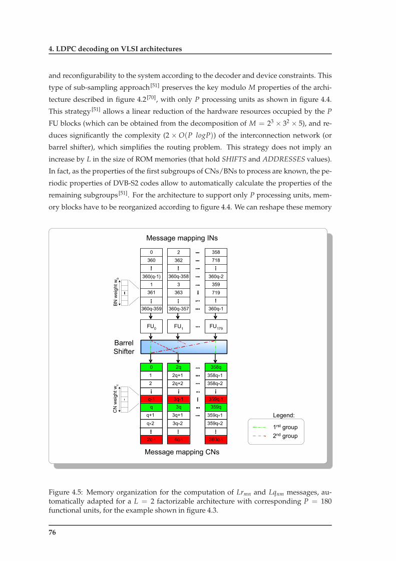
4. LDPC decoding on VLSI architectures
and reconfigurability to the system according to the decoder and device constraints. This
type of sub-sampling approach [51] preserves the key modulo M properties of the archi-
tecture described in figure 4.2 [70], with only P processing units as shown in figure 4.4.
This strategy [51] allows a linear reduction of the hardware resources occupied by the P
FU blocks (which can be obtained from the decomposition of M = 23 × 32 × 5), and re-
duces significantly the complexity (2 × O(P logP)) of the interconnection network (or
barrel shifter), which simplifies the routing problem. This strategy does not imply an
increase by L in the size of ROM memories (that hold SHIFTS and ADDRESSES values).
In fact, as the properties of the first subgroups of CNs/BNs to process are known, the pe-
riodic properties of DVB-S2 codes allow to automatically calculate the properties of the
remaining subgroups [51]. For the architecture to support only P processing units, mem-
ory blocks have to be reorganized according to figure 4.4. We can reshape these memory
358q
359q-1
359q
360q-14q-1
3q
3q-1
2q0
2q-1
q-1
q
FU0
FU179
FU1
Barrel
Shifter
Message mapping CNs
Message mapping INs
0
360
1
361
360q-359
2
362
3
363
360q-357
358
718
360q-2
719
358q+1
358q+2
2q+1
2q+2
1
2
1rst group
2nd group
Legend:
359
360q-1
359q+1
359q+23q+2
3q+1
q+2
q+1
360q-358360(q-1)
BN weight wb
CN weight wc
Figure 4.5: Memory organization for the computation of Lrmn and Lqnm messages, au-tomatically adapted for a L = 2 factorizable architecture with corresponding P = 180functional units, for the example shown in figure 4.3.
76

4.3 M-factorizable LDPC decoder for DVB-S2
blocks [51] and keep unchanged the size of the system ROM, by computing on the fly the
new SHIFTS values as a function of those initially stored in the ROM of figure 4.2 [51] for
a level of parallelism corresponding to M = 360. In the configuration [51] shown in fig-
ure 4.4, each FUi, with 0 < i < P− 1, is now responsible for processing information (IN),
parity (PN) and check nodes (CN) according to a proper memory mapping and shuffling
mechanism conveniently detailed in Appendix A. As we increase L, the smaller are the
sub-sets of the Tanner graph processed in parallel. Figure 4.5 describes the addressing
mechanisms used in the factorizable architecture for L = 2, or 180 FUs. The amount of
memory is exactly the same as in the previous architecture, but the structure is different.
There are less FUs and the corresponding memory word size decreases. But memories
have to become higher and thinner in order to hold the same information as before. This
new memory configuration will introduce benefits in area occupied by the architecture,
as it will be shown later.
Adder
Reg SUM
Channel
Adder
Reg SUM Out
+
-
Lr
> 0
Hard
Decoding
Reg SUM
FIFO +
-
Reg SUM Out
Lr
Lq
FIFO
Lq
Figure 4.6: Serial architecture for a functional unit that supports both CN and BN pro-cessing types [31,49] for the MSA.
77

4. LDPC decoding on VLSI architectures
4.3.1 Functional units
The type of processing performed by each FU is based on the MSA defined in (2.26) to
(2.31) of algorithm 2.2. Figure 4.6 shows a FU that supports both BN and CN serial pro-
cessors and figure 4.7 expands the boxplus and boxminus blocks depicted in figure 4.6.
Figure 4.8 depicts a parallel version of the FU. Considering a BN of weight wb, the BN
processor can be seen as a black box with wb + 1 inputs, from where it receives the chan-
nel information plus wb CN messages Lrmn, sent from the CNs connected to it, and with
wb + 1 outputs, through where it communicates the hard decoding decisions and sends
the wb messages Lqnm, to the CNs connected to it. The inputs are added on a recursive
manner as shown in figure 4.6. The Reg SUM register is initialized with the received
channel information. The output messages can be obtained in a parallel manner as in
figure 4.8, or using a full serial approach as shown in figure 4.6, with a new message
being obtained at each clock cycle. This implementation minimizes the hardware com-
Adder
b
aResult
Sign(a)
Sign(b)
Adder
Adder
xor
MUX
min(|a|,|b|)
Final Sign
-
+
+
+
-
+
+Comparator
abs
abs
abs
Reg
Adder
Adder
-
-
+
Result
b
aAdder
Adder
+
+
-
+
+
-min(|a|,|b|)
abs
Figure 4.7: Boxplus and boxminus sub-architectures of figure 4.6 [31,49].
plexity (measured in terms of number of logic gates) at the cost of a significant increase in
processing time (time restrictions could require an increase in the clock frequency). The
serial implementation has also the advantage of supporting the processing of a BN of any
weight, at the expense of little additional control. In a parallel version, inputs are added
78
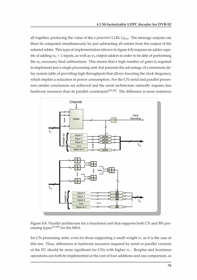
4.3 M-factorizable LDPC decoder for DVB-S2
all together, producing the value of the a posteriori LLRs Lqnm. The message outputs can
them be computed simultaneously by just subtracting all entries from the output of the
referred adder. This type of implementation (shown in figure 4.8) requires an adder capa-
ble of adding wb + 1 inputs, as well as wb output adders in order to be able of performing
the wb necessary final subtractions. This means that a high number of gates is required
to implement just a single processing unit, but presents the advantage of a minimum de-
lay system (able of providing high throughput) that allows lowering the clock frequency,
which implies a reduction in power consumption. For the CN serial and parallel proces-
sors similar conclusions are achieved and the serial architecture naturally requires less
hardware resources than its parallel counterpart [31,49]. The difference is more notorious
Adder
Lr
adder
> 0
adderadder
adder
Channel
Hard
Decoding
+
-
-
-
-
Lq
Input 0
Input w-1
Input 1
Input 2
(weight w)
+
-
-
-
-
Lq
Lr{
Input 0
Input w-1
Input 1
Input 2
(weight w) {
Figure 4.8: Parallel architecture for a functional unit that supports both CN and BN pro-cessing types [31,49] for the MSA.
for CN processing units, even for those supporting a small weight wc as it is the case of
this one. Thus, differences in hardware resources required by serial or parallel versions
of the FU should be more significant for CNs with higher wc. Boxplus and boxminus
operations can both be implemented at the cost of four additions and one comparison, as
79
4. LDPC decoding on VLSI architectures
shown in figure 4.7. Based on the proposed boxplus and boxminus hardware modules,
it is possible to adopt a serial or parallel configuration for the CN processor (similar to
the described for BN processor units). Nevertheless, the complexity of the boxplus oper-
ation on a parallel implementation requires a boxplus sum chain of all inputs according
to the figure 4.8. The advantages of one configuration compared with the other are sim-
ilar to those mentioned for the BN processor. Nevertheless, it should be noted that the
proportion of silicon area occupied by a parallel implementation with respect to a serial
implementation, in this case is significantly higher than the one for the BN processor, due
to the number of operations involved in the boxplus and boxminus processing. In fact,
the number of gates required by the boxplus and boxminus processing units is superior
to common add and subtract arithmetic operations.
The fact that only Lrmn messages represented in (2.26) are used in the processing of
CNs and, at the same time, only Lqnm messages represented in (2.29) are used in the
processing of BNs, allows simplifying the architecture, since memory can be shared by
both types of processing (one overlaps the following), as data is discarded at the end of a
computation and posterior storing in memory. During the execution of an iteration, the
decision of performing BN or CN processing should be performed by the Control unit
depicted in figures 4.2 and 4.4. The FUs proposed can be efficiently described by using a
Hardware Description Language (HDL) library tool developed [31] to automatically gen-
erate Register Transfer Level (RTL) code that produces either fully serial or fully parallel
synthesizable FU processing blocks [31,49].
The architecture proposed in this section [51] uses functional units based on the full
serial approach depicted in figure 4.6, which requires a lower number of gates (and area)
at acceptable clock frequency. Also, it supports all different code rates and frame lengths
making it fully compliant with the DVB-S2 standard [29]. This solution allows a good
compromise between throughput, algorithm complexity and hardware resources. In the
next sub-sections we present the obtained experimental results for both FPGA and ASIC
devices.
4.3.2 Synthesis for FPGA
The architecture of figure 4.4 was synthesized for Virtex-II Pro FPGAs (XC2VPxx)
from Xilinx for validation purposes. In all solutions 5 bits are used to represent data
(input values and inner messages). Table 4.1 reports the hardware resources used in
FPGAs XC2VP30, XC2VP50 and XC2VP100 for 3 different factorization levels, namely
L = {2, 4, 8}, and also the maximum frequency of operation, which can be obtained
from:
fclk_max =1
(Logic Delay + Routing Delay), (4.1)
80

4.3 M-factorizable LDPC decoder for DVB-S2
Table 4.1: Synthesis results1 for P={45, 90, 180} parallel functional units.FPGA XC2VP30 XC2VP50 XC2VP100FUs 45 90 180 45 90 180 45 90 180
L 8 4 2 8 4 2 8 4 2
Slices (%) 87 154† 292† 50 88 169† 27 50 88Flip-Flops (%) 19 38 75 11 22 43 6 11 23
LUTs (%) 81 142† 265† 46 80 153† 25 46 80BRAM (%)
(18 Kbit blocks) 132† 144† 163† 77 84 95 40 44 50Maximum Frequencyof Operation (MHz) 70.8 – – 70.8 64.1 – 70.8 74.0 73.2
Logic Delay (ns) 8.36 – – 8.36 8.68 – 8.36 7.74 5.99Routing Delay (ns) 5.77 – – 5.77 6.93 – 5.77 5.77 7.67
where Logic Delay and Routing Delay indicate maximum obtained values. Synthesis
results show that it is necessary to use at least the FPGA XC2VP50 in order to guaran-
tee the minimum memory resources required to implement all code rates and lengths
adopted in DVB-S2. However, this particular choice uses nearly only 50% of the FPGA
available slices for a 45 FU architecture. From table 4.1 we observe that it is also possible
to implement this same architecture on the lower cost FPGA XC2VP30 if we use external
memory. For a given frequency of operation fop < fclk_max, the expected throughput is
given by:
Throughput ≥f rame_length × fop
(2×W + wj − 3
)×max_iter × L
, (4.2)
where W represents the number of elements of H in the compact form as it is represented
in annexes B and C of the DVB-S2 standard [29], and wj is the weight of the IN nodes of
the code with weight j 6= 3 (see table 2.3 in chapter 2). In the architecture of figure 4.2,
a fully serial FU computes a new message per clock cycle and only stops (in bit mode)
wj− 3 cycles when switching the processing of IN nodes of weight wj to nodes of weight
w = 3. In the architecture of figure 4.4 the number of wasted clock cycles per iteration
increases by L. The XC2VP100 FPGA allows the implementation of the architecture of
figure 4.4 with 180 FUs (a factor L = 2), which multiplies the throughput approximately
by 4 times when compared to a 45 FU architecture (a factor L = 8). Figure 4.9 presents a
comparison of the maximum number of decoding iterations for each DVB-S2 LDPC code,
that can be performed on a XC2VP100 FPGA, operated at maximum clock frequency
fclk_max, and that guarantees the minimum throughput of 90 Mbps for each configuration
of the architecture, with P = {45, 90, 180} FUs. For example, the normal frame rate = 1/4
1The symbol † indicates that more than 100% of the device resources are required.
81

4. LDPC decoding on VLSI architectures
code supports more than 10 iterations for P = 45 FUs, nearly 25 iterations for P = 90
FUs, and more than 45 iterations for P = 180 FUs. By limiting the maximum number of
iterations to 15, we can observe in figure 4.10 that the minimum throughput achievable
for the 180 FUs architecture is far above the 90 Mbps. This limit is nearly achieved and in
some cases even surpassed for DVB-S2 LDPC codes in the architecture based on 90 FUs.
0 5 10 15 20 25 30 35 40 45 50
1/4
1/3
2/5
1/2
3/5
2/3
3/4
4/5
5/6
8/9
9/10
Long-Frame DVB-S2 LDPC Decoding (N=64800) with Minimum Throughput = 90 Mb/s
Maximum Number of Iterations
Cod
e R
ate
180 FUs90 FUs45 FUs
0 5 10 15 20 25 30 35 40 45 50
1/5
1/3
2/5
4/9
3/5
2/3
11/15
7/9
37/45
8/9
Maximum Number of Iterations
Cod
e R
ate
Short-Frame DVB-S2 LDPC Decoding (N=16200) with Minimum Throughput = 90 Mb/s
180 FUs90 FUs45 FUs
Figure 4.9: Maximum number of iterations [51] that can be performed with P ={45, 90, 180} functional units2, for a throughput of 90 Mbps on a XC2VP100 FPGA.
Comparing throughput for both frame lengths in figure 4.10, we realize that they
resemble similar, which on a first analysis may seem incorrect due to the fact that normal
frame (64800 bits) codes have a length 4× longer than short frame (16200 bits) ones. The
reason for this lies in the fact that throughput represents a relation between the number
of decoded bits and the time necessary to perform that operation. As the number of bits
is 4× higher, the time spent doing that processing is equally higher because the number
of edges to process increases approximately by the same amount. Although processing
time is not exactly 4× higher, its value is very close to that number. This is the reason
82

4.3 M-factorizable LDPC decoder for DVB-S2
why both throughputs approximate that much.
In the last couple of years, FPGA technology evolved and the density of new devices
is now superior to the one supported by Virtex-II Pro FPGAs. Also, new FPGA tech-
nologies support reduced internal delays which allows to achieve higher frequencies of
operation. Any of the 3 architectures proposed based on figure 4.4 can be easily sup-
ported, for example, by a recent Virtex-6 family device.
0 30 60 90 120 150 180 210 240 270 300
1/4
1/3
2/5
1/2
3/5
2/3
3/4
4/5
5/6
8/9
9/10
Minimum Throughput [Mb/s]
Cod
e R
ate
Long-Frame DVB-S2 LDPC Decoding (N=64800) with Maximum Number of Iterations = 15
180 FUs90 FUs45 FUs
0 30 60 90 120 150 180 210 240 270 300
1/5
1/3
2/5
4/9
3/5
2/3
11/15
7/9
37/45
8/9
Minimum Throughput [Mb/s]
Cod
e R
ate
Short-Frame DVB-S2 LDPC Decoding (N=16200) with Maximum Number of Iterations = 15
180 FUs90 FUs45 FUs
Figure 4.10: Minimum throughput achievable [51] on a XC2VP100 FPGA for P ={45, 90, 180} functional units2. The maximum number of iterations is 15.
4.3.3 Synthesis for ASIC
Synthesizing in ASIC technology the architecture with P = {45, 90, 180, 360} FUs
aims at finding the one which produces better power consumption and area results, while
simultaneously supporting the minimum throughput requirements. Any of the solutions
here reported supports short and normal frame lengths, even though the architecture is
2As mentioned in 2.6.2 regarding table 2.2, five DVB-S2 short frame codes don’t have constant wc weights.For this reason, five short frame rates in figures 4.9 and 4.10 are approximations of those mentioned intable 2.2 (for example, rate = 4/9 in the figures represents code with rate = 1/2 in the table).
83
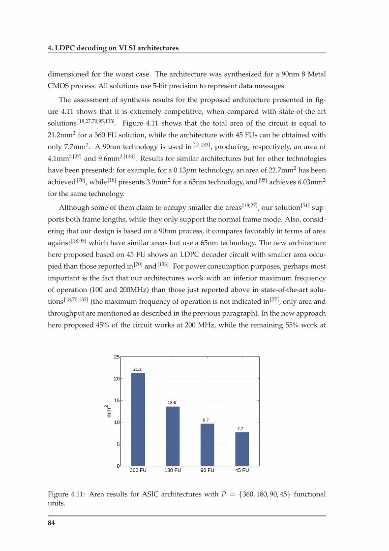
4. LDPC decoding on VLSI architectures
dimensioned for the worst case. The architecture was synthesized for a 90nm 8 Metal
CMOS process. All solutions use 5-bit precision to represent data messages.
The assessment of synthesis results for the proposed architecture presented in fig-
ure 4.11 shows that it is extremely competitive, when compared with state-of-the-art
solutions [18,27,70,95,133]. Figure 4.11 shows that the total area of the circuit is equal to
21.2mm2 for a 360 FU solution, while the architecture with 45 FUs can be obtained with
only 7.7mm2. A 90nm technology is used in [27,133], producing, respectively, an area of
4.1mm2 [27] and 9.6mm2 [133]. Results for similar architectures but for other technologies
have been presented: for example, for a 0.13µm technology, an area of 22.7mm2 has been
achieved [70], while [18] presents 3.9mm2 for a 65nm technology, and [95] achieves 6.03mm2
for the same technology.
Although some of them claim to occupy smaller die areas [18,27], our solution [51] sup-
ports both frame lengths, while they only support the normal frame mode. Also, consid-
ering that our design is based on a 90nm process, it compares favorably in terms of area
against [18,95] which have similar areas but use a 65nm technology. The new architecture
here proposed based on 45 FU shows an LDPC decoder circuit with smaller area occu-
pied than those reported in [70] and [133]. For power consumption purposes, perhaps most
important is the fact that our architectures work with an inferior maximum frequency
of operation (100 and 200MHz) than those just reported above in state-of-the-art solu-
tions [18,70,133] (the maximum frequency of operation is not indicated in [27], only area and
throughput are mentioned as described in the previous paragraph). In the new approach
here proposed 45% of the circuit works at 200 MHz, while the remaining 55% work at
360 FU 180 FU 90 FU 45 FU0
5
10
15
20
25
mm
2
21.2
13.6
9.7
7.7
Figure 4.11: Area results for ASIC architectures with P = {360, 180, 90, 45} functionalunits.
84

4.4 Optimizing RAM memory design for ASIC
100 MHz. Final circuit validation has been performed by place & route using 8 metal
layers. No time, physical or routing violations were reported, so in this stage the 45 FUs
architecture is physically validated.
At this point and due to the configurable nature of the architecture, we found room
to perform some extra optimizations. For practical purposes, and since it presented good
results for throughput and area, we adopted the configuration based on the 45 FUs as
the basis solution to be optimized. The next section shows where there is still room to
perform optimizations and how to achieve that.
4.4 Optimizing RAM memory design for ASIC
The presented architecture has been described in RTL, for P = {45, 90, 180, 360}
FUs. Figure 4.4 shows that all 4 configurations use exactly the same amount of memory,
though rearranged with different widths and heights (memory positions). The smaller
the number of P functional units adopted, the higher and thicker block memories be-
come. The complete type and amount of memories necessary for such design are [51]:
• Message memory holds internal messages calculated during each iteration of the
decoding process for all information nodes (IN). Message memory width (word
length) is given by wa = number o f FU × message precision which in this case
is wa = M× 5/L bits. The height hmm can be obtained for the worst case scenario
(code with rate = 3/5 obtained from table 2.3, where the number of edges is maxi-
mum and (N − K) = 25920). In this case, hmm = L× q× (wc − 2);
• Channel memory stores IN and PN data incoming from the channel. This memory
has the same word length as Message memory (wch = wa), and the height is given
by hch = L× 64800/M, representing the worst case (normal frame);
• PN message memory holds messages calculated during each iteration, which are
associated only with parity bits. It has the same width as Channel memory and the
height hPN is obtained for worst case scenario (code with rate = 1/4) from table 2.3,
which turns hPN = q = 135 (only one 5-bit message per each parity bit has to be
stored);
• Hard decoding memory holds IN and PN data obtained in the hard decoding phase
of processing (1-bit per FU), described by (2.30) and (2.31). The width of this mem-
ory is given by the number M of FUs of the architecture. The height hHD is obtained
from hHD = L× 64800/M.
Table 4.2 summarizes the required width and height (mem. pos.) of all memories used
in the 4 synthesized configurations. Unfortunately, sometimes RAM memory libraries of
85

4. LDPC decoding on VLSI architectures
Table 4.2: Required RAM memory size for each configuration.Type of RAM 360 FU 180 FU 90 FU 45 FU
memory (mem. pos. (mem. pos. (mem. pos. (mem. pos.× width) × width) × width) × width)
Message 648× 1800 1296× 900 2592× 450 5184× 225Channel (IN+PN) 180× 1800 360× 900 710× 450 1440× 225
PN message 135× 1800 270× 900 540× 450 1080× 225Hard decoding (IN+PN) 180× 360 360× 180 720× 90 1440× 45
Table 4.3: Physical (real) RAM memory size for each configuration.Type of RAM 360 FU 180 FU 90 FU 45 FU
memory (mem. pos. (mem. pos. (mem. pos. (mem. pos.× width) × width) × width) × width)
Message 210 × 1800 211 × 900 212 × 450 213 × 225Channel (IN+PN) 28 × 1800 29 × 900 210 × 450 211 × 225
PN message 28 × 1800 29 × 900 210 × 450 211 × 225Hard decoding (IN+PN) 28 × 360 29 × 180 210 × 90 211 × 45
standard cells do not exactly support the specified heights (memory positions) requested
in table 4.2, but rather standard dimensions which are usually a power of 2, as shown
in table 4.3. The area results obtained in the synthesis process and shown in figure 4.11,
allowed other interesting conclusions. Memories occupy nearly 97% of the circuits’ total
area. The remaining part of the circuit is occupied by the barrel shifter, functional units
and control logic. The fact that in the 4 configurations the areas are different was also a
surprise. Figure 4.11 shows these differences. As mentioned before and depicted from
figure 4.4, the total amount of memory is the same for all designs. If we realize that
they occupy a significant area of the design, we conclude that their differences should
be minimal. To analyze these differences, we first need to understand how memories
are generated and the RAM generator limitations. The architecture implemented in RTL
uses memories with large width (word length) and height (number of words, or memory
positions).
The RAM generator used can create memories that support the requested number of
words, but the maximum word width is limited to 64 bits, which is far bellow from archi-
tectural needs. To overcome this problem, B RAMs were concatenated until the required
memory width has been achieved, as shown in figure 4.12. Each RAM memory has its
own internal control logic which can address data in the working clock cycle, with its
own antenna diode protection, testing mechanisms, power rings, etc. As represented in
figure 4.12, for large words more memories are necessary, which replicates control hard-
86
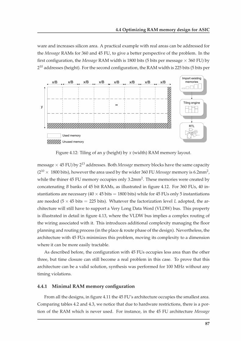
4.4 Optimizing RAM memory design for ASIC
ware and increases silicon area. A practical example with real areas can be addressed for
the Message RAMs for 360 and 45 FU, to give a better perspective of the problem. In the
first configuration, the Message RAM width is 1800 bits (5 bits per message × 360 FU) by
210 addresses (height). For the second configuration, the RAM width is 225 bits (5 bits per
U/D
Reset
B1
B4
Carry out
ENB
Counter
S1
S2
D
C ENB
Multiplexer
x/B x/B x/Bx/B
y
Used memory
Unused memory
Import existing
memories
Tiling engine
RTL
Q
Q
SET
CLR
S
R
EN
B
x/B x/Bx/Bx/B
Figure 4.12: Tiling of an y (height) by x (width) RAM memory layout.
message× 45 FU) by 213 addresses. Both Message memory blocks have the same capacity
(210× 1800 bits), however the area used by the wider 360 FU Message memory is 6.2mm2,
while the thiner 45 FU memory occupies only 3.2mm2. These memories were created by
concatenating B banks of 45 bit RAMs, as illustrated in figure 4.12. For 360 FUs, 40 in-
stantiations are necessary (40× 45 bits = 1800 bits) while for 45 FUs only 5 instantiations
are needed (5× 45 bits = 225 bits). Whatever the factorization level L adopted, the ar-
chitecture will still have to support a Very Long Data Word (VLDW) bus. This property
is illustrated in detail in figure 4.13, where the VLDW bus implies a complex routing of
the wiring associated with it. This introduces additional complexity managing the floor
planning and routing process (in the place & route phase of the design). Nevertheless, the
architecture with 45 FUs minimizes this problem, moving its complexity to a dimension
where it can be more easily tractable.
As described before, the configuration with 45 FUs occupies less area than the other
three, but time closure can still become a real problem in this case. To prove that this
architecture can be a valid solution, synthesis was performed for 100 MHz without any
timing violations.
4.4.1 Minimal RAM memory configuration
From all the designs, in figure 4.11 the 45 FU’s architecture occupies the smallest area.
Comparing tables 4.2 and 4.3, we notice that due to hardware restrictions, there is a por-
tion of the RAM which is never used. For instance, in the 45 FU architecture Message
87

4. LDPC decoding on VLSI architectures
Ch
an
ne
l m
em
ory
PN
Me
ssag
e
me
mo
ry
FU’s
control
Barrel shifterShift
calculator
SH
IFT
S
Address
calculatorIN/CN
mode
AD
DR
ES
SE
S
FU
45
FU
3
FU
2
FU
1
0
1
Message memory
5
5
5
5
5
5
5
5
5 5 5 5
VLDW BUS
Figure 4.13: Optimized 45 functional units architecture.
RAM needs 225× 5184 = 1166400 bits. But physically, we need 225× 213 = 1843200 bits,
resulting in 1843200 − 1166400 = 676800 unused bits, about 37%. This fact occurs in all
memories and for all architectures and it can be minimized using decompositions in pow-
ers of 2. From the previous example, we notice that the RAM height can be decomposed
into 5184 = 212 + 210 + 26. To minimize the unused area, we can use the concatenation
of smaller RAMs, obtaining a RAM depth near the specific architecture needs. Unfor-
tunately, after generating and concatenating the decomposed RAMs, we realize that the
area increases nearly 30% (instead of decreasing), which can be justified by the additional
number of internal RAM hardware controllers incorporated into the design. This factor is
the major responsible for increasing the area. Therefore, decomposing RAMs in powers
of 2 is not an interesting solution. However, joining together several blocks of memory
that operate in different time slots into one bigger common block of memory can become
a more efficient solution. First, we need to understand in more detail the decoder archi-
tecture with 45 FUs as depicted in figure 4.13. In Message memory of figure 4.13, each
5 bits of the word are directly connected to each FU, and consequently only one main
memory block is used. This way, only one (read or write) address is needed to transfer
88

4.4 Optimizing RAM memory design for ASIC
data to/from all FUs. This memory must be a dual port RAM, in order to allow reading
and writing during the same clock cycle. However, due to memory generator limitations
in the tools used, this type of memory was not possible to achieve. The solution adopted
consists of creating a memory operating at twice the circuit’s frequency: in the first cycle
it performs read operations; and in the second one it writes data to memory. The LDPC
decoder input data comes from an external de-interleaver module that does not work
at the same clock frequency as the LDPC decoder. To guarantee that no information is
lost, all messages delivered to the decoder must be stored in Channel memory. The PN
message memory is equally stored on a dual port RAM which, as before, due to memory
generator limitations was converted into a single RAM working at twice of the initial
frequency. In the beginning, this memory is loaded with zeros, and then it will hold data
associated with parity bits necessary in each iteration of the decoding process. Shift and
address data are loaded from an outside source into SHIFTS and ADDRESSES memories.
The values stored into these memories depend on the code rate and must be previously
calculated.
4.4.2 ASIC synthesis results for an optimized 45 FUs architecture
The floorplan with placed std cells, RAM memory and pins is presented in figure 4.15
for the optimized 45 FUs design. To translate the mentioned optimizations into area re-
quirements, the new circuit has been synthesized for the same 90nm technology used in
the original synthesis. The optimizations reduce the area of the smallest original architec-
ture nearly 20%. Synthesis results for the optimized 45 FUs version and also for the previ-
Figure 4.14: Layout of a memory with 10-bit width ×10 lines of bus address.
ously mentioned P = {360, 180, 90, 45} FUs based architectures, are listed in table 4.4 and
the areas are also compared in figure 4.16. They range from 21.2mm2 to 6.2mm2, with cor-
responding levels of power consumption of, respectively, 290mW down to 85mW. The 45
FU’s architecture optimized with an efficient RAM memory reshape presents a total area
89

4. LDPC decoding on VLSI architectures
Figure 4.15: Floorplan with placed std cells, RAM and pins for the optimized 45 func-tional units design.
of 6.2mm2 and 85mW of power consumed at a typical voltage of 1.1V (and maximum
1.32V). The estimation of power consumption was performed by considering typical val-
ues for current, voltage and temperature. This approach was followed because extreme
working conditions usually do not occur, or if they do, it is during small periods of time
which does not negatively affect the design.
360 FU 180 FU 90 FU 45 FU 45 FU opt.0
5
10
15
20
25
mm
2
21.2
13.6
9.7
7.7
6.2
less than3.4x
Figure 4.16: Area results comparing the optimized 45 FUs design.
90

4.4 Optimizing RAM memory design for ASIC
Table 4.4: ASIC synthesis results for P = {45, 90, 180, 360} parallel functional units andfor an optimized 45 functional units architecture.
360 180 90 45 45-optim.
Technology 90nm 90nm 90nm 90nm 90nmMax. voltage 1.32 v 1.32 v 1.32 v 1.32 v 1.32 vTyp. voltage 1.1 v 1.1 v 1.1 v 1.1 v 1.1 vMin. voltage 1.08 v 1.08 v 1.08 v 1.08 v 1.08 v
Max. temperature 125°C 125°C 125°C 125°C 125°CTyp. temperature 25°C 25°C 25°C 25°C 25°CMin. temperature -40°C -40°C -40°C -40°C -40°CMax. frequency 100MHz 100MHz 100MHz 100MHz 100MHz
Power 290mW 185mW 130mW 105mW 85mWCurrent 260mA 170mA 120mA 95mA 75mA
Gate count 9.6 Mgates 6.2 Mgates 4.4 Mgates 3.5 Mgates 2.8 MgatesArea 21.2mm2 13.6mm2 9.7mm2 7.7mm2 6.2mm2
Figure 4.17 facilitates assessing the dimension and complexity of this design (designs
developed for common applications in the industry of semiconductors are typically much
smaller). For example, the size of the circuit for 360 FU is comparable, in terms of the
number of gates, with an Intel® Pentium® 4 processor that requires approximately 55
millions of transistors [66] or the equivalent 14 millions of gates [73]. This LDPC decoder
design produces a chip with 9.6 millions of gates, as it is also described in table 4.4. Even
the optimized architecture with 45 FU requests 2.8 millions of gates, a value which is very
Pentium 4 360 180 90 45 45 opt. Min.0
2
4
6
8
10
12
14
16
Mill
ions
of g
ates
[66, 73]
[27]
Figure 4.17: Reference designs for gate count comparison of the ASIC based architecturesproposed, with 360, 180, 90, 45 and 45-optimized functional units.
91
4. LDPC decoding on VLSI architectures
inferior to the former but still quite significant, and very close to an architecture described
in the literature [27] that presents the minimal number of 2 millions of gates for an LDPC
decoder (for the best of our knowledge). This architecture [27] uses a 90nm CMOS tech-
nology where each NAND2 gate occupies approximately 2.1µm2. To estimate the total
number of gates of this design, we divided the total area of 4.1mm2 [27] per NAND2 gate
area to obtain an approximate value of 1.95 millions of gates. This value is also presented
as the rightest most element of figure 4.17.
Again, final circuit validation has been performed by place & route, using 8 metal
layers. No time, physical or routing violations were reported, so in this stage the 45 FU
optimized architecture is physically validated and ready to be implemented in silicon.
To accommodate place & route, it should be noted that, based on previous design ex-
perience, we estimated an increase of area equivalent to 20% (after final validation, we
realized that it could have been approximately 19%), which corresponds to a global area
of 7.4mm2 for the optimized 45 FUs architecture.
4.5 Summary
This chapter addresses the generalization of a state-of-the-art M-kernel parallel struc-
ture for LDPC-IRA DVB-S2 decoding, for any integer factor of M = 360. The proposed
method adopts a partitioned processing of sub-blocks of the Tanner graph, that keeps
unchanged the efficient message memory mapping structure without addressing unnec-
essary overheads. This architecture proves to be flexible and easily configurable accord-
ing to the decoder constraints and represents a trade-off between silicon area and de-
coder throughput. Synthesis results for FPGA devices show that a complete LDPC-IRA
decoder for DVB-S2 based on an 180 FUs architecture can be configured on a low-cost
XC2VP100 FPGA from Xilinx.
When synthesizing for ASIC technology the limitations in terms of number of gates
naturally no longer become important, and larger architectures could be tested. Never-
theless, this approach aims at finding microcircuits with the smallest possible die area
and lower power consumption, that still ensure minimum throughput requirements for
all DVB-S2 codes. Under this context, 5 configuration designs with different number of
processing units have been implemented. They range from 360 to 45 FUs which repre-
sents, respectively, an equivalent area occupied of 21.2 and 7.7mm2. Although the process
of generating RAM memories imposes constraints, the investigation carried out under
this thesis allowed achieving several interesting conclusions, that were applied into the
design of the LDPC decoder circuit. Re-dimensioning and rearrangements in the order
how memory blocks are grouped together allowed reducing the global area of the circuit
92
4.5 Summary
to a value as low as 6.2mm2. This shows the competitiveness of the architecture when
compared with state-of-the-art solutions. Moreover, the maximum frequency of opera-
tion of the design here proposed is smaller than those reported by competitors, which
justifies the low levels of power consumption achieved.
93

4. LDPC decoding on VLSI architectures
94

"If you were plowing a field, which would you rather use? Two strong oxen or 1024chickens?"
Seymour Cray


5LDPC decoding on multi- and
many-core architectures
Contents5.1 Multi-core architectures and parallel programming technologies . . . . 99
5.2 Parallel programming strategies and platforms . . . . . . . . . . . . . . 103
5.2.1 General-purpose x86 multi-cores . . . . . . . . . . . . . . . . . . . 103
5.2.2 The Cell/B.E. from Sony/Toshiba/IBM . . . . . . . . . . . . . . . 1035.2.3 Generic processing on GPUs with Caravela . . . . . . . . . . . . . 1055.2.4 NVIDIA graphics processing units with CUDA . . . . . . . . . . 108
5.3 Stream computing LDPC kernels . . . . . . . . . . . . . . . . . . . . . . 109
5.4 LDPC decoding on general-purpose x86 multi-cores . . . . . . . . . . . 111
5.4.1 OpenMP parallelism on general-purpose CPUs . . . . . . . . . . 1115.4.2 Experimental results with OpenMP . . . . . . . . . . . . . . . . . 112
5.5 LDPC decoding on the Cell/B.E. architecture . . . . . . . . . . . . . . . 114
5.5.1 The small memory model . . . . . . . . . . . . . . . . . . . . . . . 1155.5.2 The large memory model . . . . . . . . . . . . . . . . . . . . . . . 117
5.5.3 Experimental results for regular codes with the Cell/B.E. . . . . . 1215.5.4 Experimental results for irregular codes with the Cell/B.E. . . . . 126
5.6 LDPC decoding on GPU-based architectures . . . . . . . . . . . . . . . 127
5.6.1 LDPC decoding on the Caravela platform . . . . . . . . . . . . . . 1285.6.2 Experimental results with Caravela . . . . . . . . . . . . . . . . . 1325.6.3 LDPC decoding on CUDA-based platforms . . . . . . . . . . . . . 134
5.6.4 Experimental results for regular codes with CUDA . . . . . . . . 1385.6.5 Experimental results for irregular codes with CUDA . . . . . . . 143
5.7 Discussion of architectures and models for parallel LDPC decoding . 145
97

5. LDPC decoding on multi- and many-core architectures
5.8 Summary . . . . . . . . . . . . . . . . . . . . . . . . . . . . . . . . . . . . . 147
98

5.1 Multi-core architectures and parallel programming technologies
In chapter 3 we analyzed the decoding complexity of the Sum-Product Algorithm
(SPA) and Min-Sum Algorithm (MSA). The required number of operations depicted in
figures 3.1 and 3.2 shows that high performance parallel computing should be considered
to execute such intensive processing. To achieve real-time computation they can be per-
formed by using dedicated Very Large Scale Integration (VLSI) processors based on Field
Programmable Gate Array (FPGA) or Application Specific Integrated Circuits (ASIC),
as described in chapter 4. However, hardware represents non-flexible and non-scalable
dedicated solutions [137] [27], that require many resources and long development times.
More flexible solutions for Low-Density Parity-Check (LDPC) decoding using Digital
Signal Processor (DSP)s [53] or Software Defined Radio (SDR) programmable hardware
platforms [108] have already been proposed.
In this chapter we exploit the advances in powerful low-cost and widespread paral-
lel computing architectures for achieving high performance LDPC decoding. Although
general-purpose x86 multi-cores show modest performances for achieving real-time LDPC
decoding for most of the applications, they allowed to show that the solutions here pro-
posed are scalable. From the set of multi-core based architectures analyzed in this thesis,
the Cell Broadband Engine (Cell/B.E.) and Graphics Processing Units (GPU) emerge as
flexible highly parallel architectures. Because they represent programmable solutions,
they offer the possibility of increased productivity at low-cost, namely to impact the per-
formance of demanding algorithms such as the LDPC decoders analyzed in this thesis.
5.1 Multi-core architectures and parallel programming technolo-gies
Until a few years ago, general-purpose single-core based processors were unable
to handle the computational complexity of LDPC codes in real-time. The throughputs
achieved using this type of processors were below the hundreds of Kbps [32], which does
not represent a solution powerful enough to be considered as a consistent alternative for
LDPC decoding. But the evolution of processor architectures supported on the scaling
up of the technology according to Moore’s Law has lead to the actual multi-core super-
scalar processors. Mainly due to frequency of operation, power consumption and heat
dissipation constraints, the trade-off speed/power, a fundamental relation of multi-core
processors, showed that it would be more efficient to use two or more processing cores
on a single processor, rather than to continue increasing the frequency of operation. The
integration of multiple cores into a single chip has become the new trend to increase
processor performance. These architectures [12] require the exploitation of parallelism to
achieve high performance.
99

5. LDPC decoding on multi- and many-core architectures
Table 5.1: Overview of recent multi-core platforms1.Platform # cores Performance Mem. band. Homog.
Intel 6-core Dunnington [65] 6 < 51 GFLOPS2 1.07 GT/s3 Yes
Intel Xeon Nehalem 2x-Quad 8 – – Yes
Tilera 64-core Tile64 [119] 64 443 GOPS 4TB/s Yes
STI Cell/B.E. [24] 9 > 200 GFLOPS 204.8 GB/s No
NVIDIA 8800 GTX [96] 128 350 GFLOPS 86.4 GB/s Yes
ATI/AMD Radeon HD 2900 XT [5] 320 475 GFLOPS 105.6 GB/s Yes
Multi-core architectures have evolved from dual or quad-core to tera-scale systems,
supporting multi-threading, a powerful technique to hide memory latency, while at the
same time provide larger Single Instruction Multiple Data (SIMD) units for vector pro-
cessing [48]. New parallel programming models and programming tools have been de-
veloped for multi-core architectures, namely common programming models that allow
the user to program once and execute on multiple platforms, such as RapidMind [105].
Common general-purpose multi-core processors replicate a single core in a homogeneous
way, typically with a x86 instruction set, and provide shared memory hardware mech-
anisms. They support multi-threading and share data at a certain level of the memory
hierarchy, and can be programmed at a high level by using different software technolo-
gies [71], such as OpenMP [21] which provides an effective and relatively straightforward
approach for programming general-purpose multi-cores.
Presently, companies like Intel, Tilera, IBM, NVIDIA or ATI/AMD are manufacturing
systems based on multi-core processors with typically from 2 superscalar cores up to a
few hundreds of simple cores. Table 5.1 presents some examples of architectures that
incorporate multiple cores. The Dunnington processor [65] is a variant of the Intel Xeon
family (also known as Penryn processor) with a peak performance that does not allow
to achieve real-time LDPC decoding for the most demanding cases (see figure 3.2). The
distributed nature of the Tilera 64-cores processor Tile64 [119] is supported by multiple
x-y orthogonal buses, an efficient mesh that allows each core to communicate in parallel
along four different directions thus producing a very interesting aggregate bandwidth of
4 TB/s. Nonetheless, it represents an expensive solution where important parameters,
such as the number of sustained floating-point operations per second, remain unknown.
1All information indicated in table 5.1 represents peak performance values. The values indicated inGFLOPS (floating-point operations) refer to single-precision operations. The omitted values were unavail-able.
2The performance value for the Intel 6-core Dunnington processor indicated in table 5.1 represents anupper bound estimate. The peak performance values were not available.
3GT/s represents Giga Transfer (GT) per second; the value is provided by the manufacturer.
100
5.1 Multi-core architectures and parallel programming technologies
On the other hand, GPUs from NVIDIA [96] or ATI/AMD [5] have hundreds of cores and a
shared memory hierarchy which provide high computational power that can be exploited
efficiently to other types of processing not only limited to graphics processing.
Mainly due to demands for visualization technology in the industry of games, the
performance of GPUs has undergone increasing performances over the last decade. With
many cores driven by a considerable memory bandwidth, recent GPUs are targeted for
compute-intensive, multi-threaded, highly-parallel computation. Researchers in high
performance computing fields are applying their huge computational power to general
purpose applications (General Purpose Computing on GPUs (GPGPU)) [15,37,45,54,98], al-
lowing higher levels of performance in Personal Computer (PC) systems [4,72]. Moreover,
a cluster-based approach using PCs with high performance GPUs has been already re-
ported [42]. Owens et al. summarize the state-of-the-art and describe the latest advances
performed by the scientific community in GPGPU [99]. At the compiler level, Buck et al.
introduced important improvements, such as the extensions to the C language known
as Brook for GPUs [20], which allows to perform general purpose computation on pro-
grammable graphics hardware. However, to apply GPUs to general purpose applica-
tions, we need to manage very detailed code to control the GPU’s hardware. To hide this
complexity from the programmer, several programming interfaces and tools [89], such as
the Compute Unified Device Architecture (CUDA) from NVIDIA [97], the Close to the
metal (CTM) interface (replaced by the ATI Stream SDK) from AMD/ATI [6], or the Car-
avela platform [126] have been developed. CUDA and CTM represent dedicated program-
ming tools for specific GPUs with a strong potential to improve the computational ef-
ficiency [47]. CUDA provides a new hardware and software architecture for managing
computations on GPUs [22,57,80,130] with the Tesla architecture from NVIDIA. The Caravela
platform [125,126] holds the interesting property of being the first generalist and powerful
programming tool that operates independently of the operating system and GPU manu-
facturer. Recently standardized, the OpenCL framework [55] allows to write parallel pro-
grams for execution across heterogenous platforms that include CPUs, GPUs and other
types of processors.
Also pushed by audiovisual needs in the industry of games, emerged the Sony, Toshiba
and IBM (STI) Cell/B.E. [24] listed in table 5.1. It is characterized by a heterogeneous vec-
torized Single Instruction Multiple Data (SIMD) multi-core architecture composed by one
main PowerPC Processor Element (PPE) that communicates very efficiently [2] with eight
Synergistic Processor Element (SPE)s that operate without sharing memory. Each SPE
holds a small amount of local memory for data and code, which is conveniently exploited
by a vectorized SIMD oriented architecture [60]. Data transfers between PPE and SPE
are performed efficiently by using Direct Memory Access (DMA) mechanisms. Driven
101

5. LDPC decoding on multi- and many-core architectures
Table 5.2: Overview of software technologies for multi-cores [71].Software Corporation Target Language/
Technology architecture Library
CUDA NVIDIA NVIDIA GPU Language (C)
BROOK+ AMD/ATI AMD/ATI GPU Language (C)
Cell SDK IBM Cell/B.E. Library (C)
OpenMP ARB Group multi-core CPU Library (C, FORTRAN)
OpenCL Stand. Khronos Group GPU, CPU, FPGA Language (C)
PCT MATHWORKS multi-core CPU Language (Matlab)
by a considerable memory bandwidth, the Cell/B.E. processor powers IBM Cell Blade
servers, and supports also the PlayStation3 (PS3) platform. The PS3 can be operated with
Linux-based operating systems, thus it can be used beyond gaming [103], providing low-
cost high-performance professional computing platforms very attractive for demanding
scientific applications [3,76].
Table 5.2 presents a subset of the most important technologies used in the program-
ming of multi-core platforms [71]. It shows some of their main properties, namely the
programming language that each parallel platform supports. The C language emerges
as a commonly supported language. Other programming languages such as C++, FOR-
TRAN, PYTHON or JAVA are also supported by some multi-core architectures and paral-
lel programming models. At the same time, these architectures support data-parallelism
and most of them also support task-parallelism.
From the set of architectures based on multi-core processors presented in table 5.1,
the low-cost and worldwide disseminated Cell/B.E. and GPUs supported by CUDA are
flexible highly parallel architectures which support data and thread levels of parallelism,
and can be efficiently programmed using the conventional C language (see table 5.2)
to perform LDPC decoding. Also, common general-purpose x86 multi-core processors,
supported by an increasing number of cores, can address scalable implementations of
parallel algorithms in future versions of the architectures. For all these reasons, they
were selected in this thesis as the processing platforms to develop and implement pro-
grammable LDPC decoders.
The GPU is not an autonomous processing system. A very important aspect is re-
lated with the need of transferring data from the host (Central Processing Unit (CPU)) to
the device (GPU), and in the opposite direction at the end of processing. The comput-
ing platforms used in this test are PCs that showed peak data transfers of approximately
1.2 GByte/s, experimentally measured between the host and the device connected to the
102

5.2 Parallel programming strategies and platforms
workstation through a Peripheral Component Interconnect Express (PCIe) bus.
5.2 Parallel programming strategies and platforms
The two types of intra-codeword (Definition 3.1) and multi-codeword (Definition 3.2)
parallelism, defined in subsection 3.3, can be applied differently to distinct parallel com-
puting architectures. In this thesis we exploit both concepts and show how they can
be efficiently applied, depending on the target architecture. General-purpose x86 multi-
cores can make use of them separately, while they can be combined to achieve better
performance in other architectures, such as in GPUs and the Cell/B.E., as described in
the next subsections.
5.2.1 General-purpose x86 multi-cores
The number of cores of general-purpose x86 multi-cores typically ranges from 2 to
16 and includes different levels of hardware-managed cache memory [74]. In these ar-
chitectures memory cache coherency mechanisms are provided to support the shared-
memory parallel programming model. Moreover, the internal cache shared by all cores
allows efficient data transfers and synchronization between them. These processors can
be programmed by using POSIX Threads (pthreads) or, at a higher level, the OpenMP
programming interface [21].
Applications that exploit the parallel processing of matrices in general-purpose x86
multi-cores using OpenMP can be found in the literature [8,22]. For example, they de-
scribe the multiplication of matrices [8] and, in particular, of sparse-matrices [110]. Also,
several digital signal processing algorithms such as the Fast Fourier Transform (FFT), or
LU matrix decomposition4 have been parallelized using OpenMP directives [14]. How-
ever, research for performing parallel LDPC decoding in this type of architectures has
not been reported yet.
5.2.2 The Cell/B.E. from Sony/Toshiba/IBM
The Cell/B.E. is an heterogeneous processor [24,60] composed by one main 64-bit PPE
that communicates with eight SPEs each having 256 KByte of local storage (LS) memory
for data and program, and a 128-bit wide vectorized SIMD within-a-register (SWAR)
oriented architecture as depicted in figure 5.1. Data transfers between the PPE (that
accesses main memory) and SPE are performed by using efficient DMA that offload
4In linear algebra, the LU matrix decomposition [14] represents a matrix as the product of a lower triangu-lar matrix and an upper triangular matrix. This product sometimes involves a permutation matrix as well,and is used in numerical analysis to calculate the determinant or solve systems of linear equations.
103

5. LDPC decoding on multi- and many-core architectures
SynergisticProcessorElement
Element Interconnect Bus
SPE SPE SPE
SPE SPE SPE SPE
SPE
PPE Memory Interface Controller
Broadband Engine Interface
PowerPCProcessorElement
Instruction pool
Datapool
32-bit
128-bit
{
Figure 5.1: The Cell/B.E. architecture.
the processors from the time consuming task of moving data. The Memory Interface
Controller (MIC) controls the access to the main memory, with a bandwidth that nearly
reaches 4.2 GByte/s [2].
Differently from shared memory based architectures such as x86 multi-cores or GPUs,
in the Cell/B.E. data is loaded from the main memory into the LS of a SPE and vice-versa.
Data locality has to be individually exploited in each SPE, releasing to the programmer
the burden of developing strategies to avoid contention due to memory accesses. An
Output n-1
Processing n
Input n+1
Processing n+1
Output n Input n+2 ….. Pipeline DMA
Pipeline Computation
Output n-2
Processing n-1
Input n
(time)
Iteration n
Figure 5.2: Double buffering showing the use of the two pipelines (for computation andDMA).
important restriction in such architectures is related with the limited amount of local
memory [24], which in practice may lead to situations where data and code do not fit com-
pletely into the LS of a single SPE. In that case, the processing has to be performed by
successively partitioning the algorithm, which increases the number of data communica-
tions between the PPE and SPEs. The DMA latency can have a critical role in the perfor-
mance, but its impact can be reduced by using double-buffering techniques as depicted
in figure 5.2.
Parallel computing on the Cell/B.E. has been mostly investigated for video applica-
104

5.2 Parallel programming strategies and platforms
tions, such as motion estimation [91], MPEG decoders [26], or feature extraction for tracking
purposes in computer vision [116]. Also, there are approaches to solve systems of linear
equations by exploiting single- and double-precision accuracy using appropriate refine-
ment techniques on the Cell/B.E. [75]. In this work we open a novel frontier by developing
parallel LDPC decoders in this type of distributed memory architecture.
5.2.3 Generic processing on GPUs with Caravela
Among the programming tools and environments developed for GPGPU are the Car-
avela interface tool [126], a general programming interface, based on a stream-based com-
puting model [68] that can use any GPU as co-processor. Caravela does not directly in-
teract with the GPU hardware, but it has a software layer that operates on the top of the
GPU driver, which makes it a generic programming interface tool independent of the
operating system and GPU manufacturer. The graphics pipeline of a GPU consists of
several stages as depicted in figures 5.3 and 5.4. A graphics runtime such as DirectX or
Rasterizer
(Interoperation of vertices)
Display to screen
Pixel processor
(Coloring objects with
textures)
Textures for objects
Vertex processor
(Mapping vertices to a
global virtual world)
Figure 5.3: Vertex and pixel processing pipeline for GPU computation [126].
OpenGL is used to control GPU hardware. The CPU sends a data stream of vertices of
graphics objects to a vertex processor that computes resizing or perspective of the objects
calculating rotations and transformations of the coordinates, and generates new vertices.
A rasterizer receives the new vertices, interpolates it, and generates data corresponding
to the pixels to be displayed. Then, a pixel processor receives this data and computes the
color applying texture data received from the CPU side. Finally, an image with graph-
ics objects is ready to be displayed on a video screen. Because in GPUs, namely the old
ones, there is no access to output data data of the vertex processor and the rasterizer is
not programmable but directly implemented in hardware, general-purpose applications
generally only use pixel processors, mapping the I/O data streams to textures.
Caravela has been developed [126] to allow the parallelization of computationally de-
105
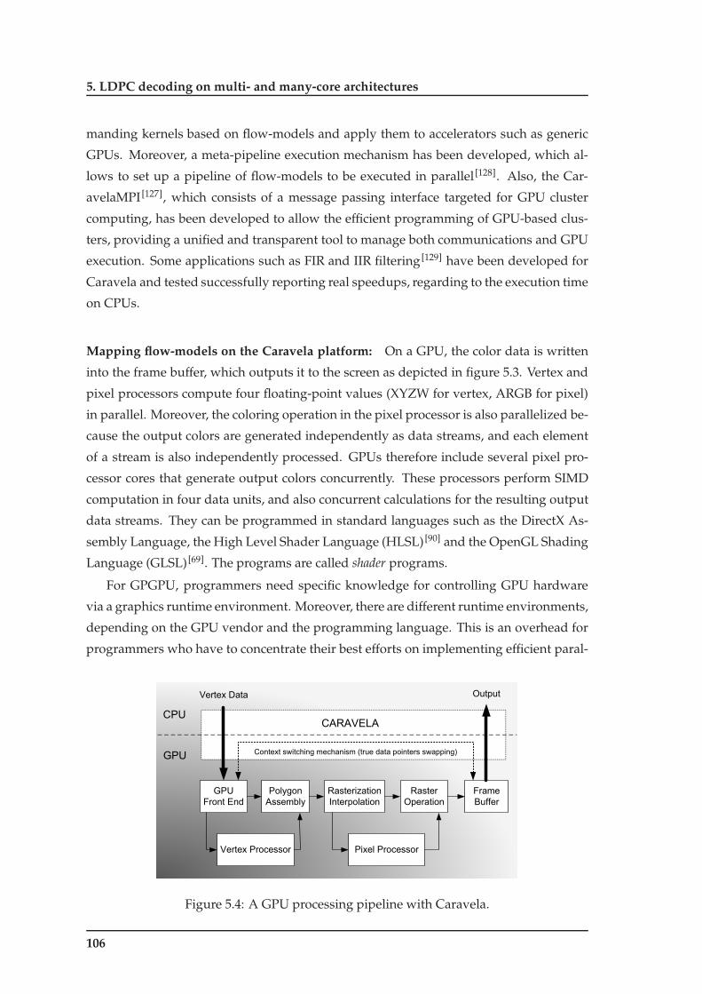
5. LDPC decoding on multi- and many-core architectures
manding kernels based on flow-models and apply them to accelerators such as generic
GPUs. Moreover, a meta-pipeline execution mechanism has been developed, which al-
lows to set up a pipeline of flow-models to be executed in parallel [128]. Also, the Car-
avelaMPI [127], which consists of a message passing interface targeted for GPU cluster
computing, has been developed to allow the efficient programming of GPU-based clus-
ters, providing a unified and transparent tool to manage both communications and GPU
execution. Some applications such as FIR and IIR filtering [129] have been developed for
Caravela and tested successfully reporting real speedups, regarding to the execution time
on CPUs.
Mapping flow-models on the Caravela platform: On a GPU, the color data is written
into the frame buffer, which outputs it to the screen as depicted in figure 5.3. Vertex and
pixel processors compute four floating-point values (XYZW for vertex, ARGB for pixel)
in parallel. Moreover, the coloring operation in the pixel processor is also parallelized be-
cause the output colors are generated independently as data streams, and each element
of a stream is also independently processed. GPUs therefore include several pixel pro-
cessor cores that generate output colors concurrently. These processors perform SIMD
computation in four data units, and also concurrent calculations for the resulting output
data streams. They can be programmed in standard languages such as the DirectX As-
sembly Language, the High Level Shader Language (HLSL) [90] and the OpenGL Shading
Language (GLSL) [69]. The programs are called shader programs.
For GPGPU, programmers need specific knowledge for controlling GPU hardware
via a graphics runtime environment. Moreover, there are different runtime environments,
depending on the GPU vendor and the programming language. This is an overhead for
programmers who have to concentrate their best efforts on implementing efficient paral-
GPU
Front End
Polygon
Assembly
Rasterization
Interpolation
Raster
Operation
Frame
Buffer
Vertex Processor Pixel Processor
Vertex Data Output
CPU
GPU
CARAVELA
Context switching mechanism (true data pointers swapping)
Figure 5.4: A GPU processing pipeline with Caravela.
106

5.2 Parallel programming strategies and platforms
Output0
Output1
Output2
Input4
Input5
Input6
"Kernel"
Input Data Stream(s) Constant Values
Output Data Stream(s)
OpInput3 Constant0
"Processor" Memory
effect
Figure 5.5: Structure of Caravela’s flow-model.
lel algorithms in a shader program. To solve this disparity in programming GPU-based
applications, the Caravela platform [126] has been developed for GPGPU, and is publicly
available at the web site [125]. The Caravela platform mainly consists of a library that sup-
ports an Application Programming Interface (API) for GPGPU. The execution unit of the
Caravela platform is based on the flow-model. As figure 5.5 shows, the flow-model is
composed of input/output data streams, constant parameter inputs and a pixel shader
program or kernel, which fetches the input data streams and processes them to generate
the output data streams. The application program in Caravela is executed as stream-
based computation. Although input data streams of the flow-model can be accessed
randomly because they are based on memory buffers accessible to the program that uses
the data, output data streams are sequences of data elements. The designation "pixel" for
a unit of the I/O buffer is used because the pixel processor processes input data for every
pixel color. A flow-model unit has defined the number of pixels for the I/O data streams,
the number of constant parameters, the data type of the I/O data streams, the pixel shader
program and the requirements for the targeted GPU. The "memory effect" is not available
in hardware, which means that we cannot store temporary results during the processing,
for example, of successive operations. To overcome this dificulty, data copy or pointer
manipulation techniques have been implemented in Caravela [129]. To give portability
to the flow-model, these items are packed into an Extensible Markup Language (XML)
file. This mechanism allows the use of a flow-model unit located in a remote computer,
simply by fetching the XML file.
107

5. LDPC decoding on multi- and many-core architectures
5.2.4 NVIDIA graphics processing units with CUDA
Recent Tesla GPUs from NVIDIA are based on a unified architecture, which repre-
sents an evolution from previous streaming architectures, where geometry, pixel and ver-
tex programs share common stream processing resources. The two GPUs from NVIDIA
herein adopted have 16 or 30 multiprocessors, each one consisting of 8 cores as depicted
in figure 5.6, which makes a total of 128 stream processors available in one case and 240
in the other, with 8192 or 16384 dedicated registers per multiprocessor [97], respectively.
These GPUs provide shared memory on each multiprocessor that allows to efficiently
exploit data parallelism. Each multiprocessor holds a 16 KByte shared memory block.
Data-parallel processing is exploited by executing a kernel in parallel through mul-
tiple threads in the available cores. CUDA [97] defines an API and provides a runtime
environment and libraries to easily program these more recent GPUs from NVIDIA [97].
The execution of a kernel on a GPU is distributed across a grid of thread blocks with
adjustable dimensions. Each multiprocessor, as depicted in figure 5.6, has several cores
that can control more than one block of threads. Each block is composed by a maxi-
mum of 512 threads that execute the kernel synchronously with threads organized in
groups of warps, and following a Single Instruction Multiple Thread (SIMT) approach:
the warp size is 32 threads and each of the multiprocessors time-slices the threads in a
warp among its 8 stream processors. However, allowing the existence of inconvenient
GPU
SP SP
SPSP
SP SP
SPSP
Shared
Memory
Multiprocessor
SP SP
SPSP
SP SP
SPSP
Shared
Memory
Multiprocessor
SP SP
SPSP
SP SP
SPSP
Shared
Memory
Multiprocessor
Interconnecting Network
Global Memory
Host CPU Host MemoryCPU
Interface
Figure 5.6: A compute unified Tesla GPU architecture with 8 stream processors (SP) permultiprocessor.
108

5.3 Stream computing LDPC kernels
divergent threads inside a warp, or using a number of threads smaller than 32, can cause
a wasting of resources or making them temporarily idle. Understanding how threads
are grouped into warps is fundamental to choose the best block size configuration. Also,
the number of threads per block has to be programmed according to the specificities of
the algorithm and the number of registers available on the GPU, in order to guarantee
that enough physical registers are allocated to each thread. All threads inside the same
block can share data through the fast shared memory block, which minimizes the need
for expensive accesses to global memory. They can also synchronize execution at specific
synchronization barriers inside the kernel, where threads in a block are suspended until
they all reach that point.
CUDA became very popular among the scientific community in the last couple of
years, fostering more efficient processing of algorithms based on intensive computation.
The literature already presents cases of applications accelerated more than an order of
magnitude [4] using this type of architecture [15,45,54,99], as compared to processing times
obtained with conventional CPUs or even with CPUs using OpenMP [22]. Regarding the
processing related with LDPC decoding, i.e. that involves calculations over matrices, and
more specifically considering large data sets which can benefit most from parallelization,
we can find parallel algorithms ranging from sparse matrix solvers [15] to belief propaga-
tion for stereo vision [19] implemented on GPUs. CUDA has fostered this increase of per-
formance even further [22], allowing new parallel computing experiences [47], where video
and image research [91,130] naturally have quickly assumed an important role. Neverthe-
less, the expected rise of the number of cores may also produce side effects [89], namely
the traffic congestion caused by intensive accesses to memory, which represents a limiting
factor in achieving performance or the scalability of algorithms.
5.3 Stream computing LDPC kernels
The Synchronous Data Flow (SDF) graph in figure 5.7 represents the computation of
an LDPC decoder. The complete updating of CNs is performed by kernel 1 and alter-
nates with the updating of BNs in kernel 2. Kernel 1 receives at the input data stream p0
representing the initial probabilities pn (algorithms 2.1 and 2.2) and another stream rep-
resenting HBN data structures (section 3.3.3), to perform the SPA/MSA horizontal pro-
cessing as indicated in (2.18) to (2.19), or (2.26) to (2.28)). It produces the output stream
r0 which is one of the input streams feeding kernel 2, that also receives the HCN data
structure (section 3.3.3) and produces the output stream q0. HCN is necessary to perform
the SPA/MSA vertical processing as indicated in (2.20) to (2.21), or in (2.29). The pair ker-
nel 1 and kernel 2 completes one iteration and is repeated i times for an LDPC decoder
109

5. LDPC decoding on multi- and many-core architectures
performing i iterations. After the final iteration, the last kernel conveys the codeword.
Kernel 1p0
r0
HCN
HBN
Kernel 2q0
qi-1
Kernel 1ri-1
HCN
HBN
Kernel 2
Data
transfer
Data
transfer
Data
transfer
Data
transfer
Data
transfer
Computation Computation Computation Computation
Figure 5.7: SDF graph for a stream-based LDPC decoder: the pair kernel 1 and kernel 2is repeated i times for an LDPC decoder performing i iterations.
In each kernel, data elements can be read sequentially but have to be stored in non-
contiguous positions (or vice-versa), which defines expensive random memory accesses.
These costly write operations demand special efforts from the programmer in order to
efficiently accommodate them in parallel architectures with distinct levels of memory
hierarchy. Applied to kernel 1 and kernel 2, the stream-based compact data structures
shown in figure 3.12 make the SPA/MSA suitable to run on a parallel processing plat-
form. The analysis of figure 5.7 shows a message-passing schedule based on flooding
schedule. This approach was detailed in subsection 3.3.2 and is adopted for the imple-
mentations described in this chapter.
Table 5.3: Types of parallelism on multi-core platforms5.Platform SIMD SPMD Multi/Intra-codeword
Intel Xeon Nehalem 2x-Quad Y Y Y/Y
STI Cell/B.E. [24] Y N Y/N6
NVIDIA 8800 GTX [96] Y7 Y Y/Y
Table 5.3 shows the stream-based parallel approaches exploited for LDPC decoding
on the considered platforms. The parallelization approaches for LDPC decoding ex-
ploit the properties of each architecture, and are proposed for a heterogeneous Cell/B.E.
SIMD vectorized distributed memory architecture, that exploits data locality, and also
for shared memory multi-core based GPU architectures using CUDA that support multi-
threading, or alternatively use the Caravela interface. Moreover, the general-purpose
parallel approaches here proposed can be applied to other multi-core architectures such
as, for example, x86 general-purpose CPUs.
5These platforms were selected under the scope of this thesis.6The Cell/B.E. exploits intra-codeword parallelism only in the large memory model.7In this case it is called SIMT.
110
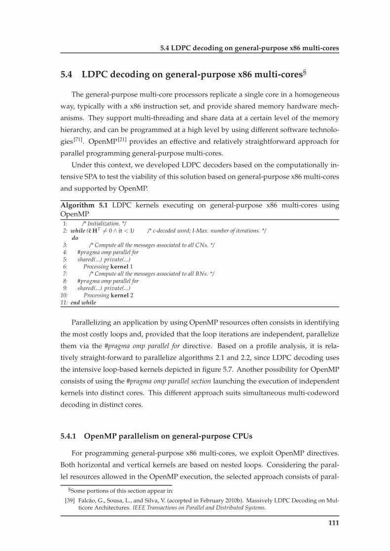
5.4 LDPC decoding on general-purpose x86 multi-cores
5.4 LDPC decoding on general-purpose x86 multi-cores§
The general-purpose multi-core processors replicate a single core in a homogeneous
way, typically with a x86 instruction set, and provide shared memory hardware mech-
anisms. They support multi-threading and share data at a certain level of the memory
hierarchy, and can be programmed at a high level by using different software technolo-
gies [71]. OpenMP [21] provides an effective and relatively straightforward approach for
parallel programming general-purpose multi-cores.
Under this context, we developed LDPC decoders based on the computationally in-
tensive SPA to test the viability of this solution based on general-purpose x86 multi-cores
and supported by OpenMP.
Algorithm 5.1 LDPC kernels executing on general-purpose x86 multi-cores usingOpenMP1: /* Initialization. */2: while (c HT 6= 0 ∧ it < I) /* c-decoded word; I-Max. number of iterations. */
do3: /* Compute all the messages associated to all CNs. */4: #pragma omp parallel for5: shared(...) private(...)6: Processing kernel 17: /* Compute all the messages associated to all BNs. */8: #pragma omp parallel for9: shared(...) private(...)
10: Processing kernel 211: end while
Parallelizing an application by using OpenMP resources often consists in identifying
the most costly loops and, provided that the loop iterations are independent, parallelize
them via the #pragma omp parallel for directive. Based on a profile analysis, it is rela-
tively straight-forward to parallelize algorithms 2.1 and 2.2, since LDPC decoding uses
the intensive loop-based kernels depicted in figure 5.7. Another possibility for OpenMP
consists of using the #pragma omp parallel section launching the execution of independent
kernels into distinct cores. This different approach suits simultaneous multi-codeword
decoding in distinct cores.
5.4.1 OpenMP parallelism on general-purpose CPUs
For programming general-purpose x86 multi-cores, we exploit OpenMP directives.
Both horizontal and vertical kernels are based on nested loops. Considering the paral-
lel resources allowed in the OpenMP execution, the selected approach consists of paral-
§Some portions of this section appear in:
[39] Falcão, G., Sousa, L., and Silva, V. (accepted in February 2010b). Massively LDPC Decoding on Mul-ticore Architectures. IEEE Transactions on Parallel and Distributed Systems.
111

5. LDPC decoding on multi- and many-core architectures
lelizing the outer-most loop of the costly operations defined in (2.18) to (2.21) or (2.26) to
(2.29), thus reducing the parallelization overheads, as depicted in algorithm 5.1. The loop
data accesses were analyzed in order to identify shared and private variables. This ap-
proach uses the #pragma omp parallel for directive to separately parallelize the processing
of kernels 1 and 2 in algorithms 2.1 or 2.2.
Algorithm 5.2 Multi-codeword LDPC decoding on general-purpose x86 multi-cores us-ing OpenMP1: /* launch decoder #1. */2: #pragma omp parallel section3: LDPC_decoder#1();4: ...5: /* launch decoder #N. */6: #pragma omp parallel section7: LDPC_decoder#N();
An alternative approach uses the #pragma omp parallel section directive to launch sev-
eral decoders in parallel, which allows to achieve multi-codeword LDPC decoding, as
represented in algorithm 5.2. In this case, the different cores do not need to share data,
neither must be synchronized upon completion of the execution of all kernels. Here, each
LDPC decoder executes at its own speed and it does not depend on the other kernels.
5.4.2 Experimental results with OpenMP
Experimental setup: To evaluate the performance of the proposed parallel stream-based
LDPC decoder, an 8 core Intel Xeon Nehalem 2x-Quad E5530 multiprocessor running at
2.4 GHz with 8 MByte of L2 cache memory was selected. The general-purpose x86 multi-
cores were programmed using OpenMP 3.0 directives and compiled with the Intel C++
Compiler (version 11.0). The experimental setup is depicted in table 5.4 and matrices
under test are presented in table 5.5.
Table 5.4: Experimental setupx86 CPU
Platform Intel Xeon Nehalem 2x-QuadLanguage C + OpenMP 3.0
OS Linux (Suse) kernel 2.6.25Number of cores 8
Clock freq. 2.4GHzMemory 8MB (L2 cache)
Experimental results with general-purpose x86 multi-cores using OpenMP: The re-
sults presented in table 5.6 were achieved using algorithms 2.1 and 5.1. However, it
112

5.4 LDPC decoding on general-purpose x86 multi-cores
Table 5.5: Parity-check matrices H under test for the general-purpose x86 multi-coresMatrix Size Edges Edges/row Edges/col.)
(M× N) (wc ×M) (wc) (wb)
o1 512× 1024 3072 {6} {3}o2 4000× 8000 24000 {6} {3}
should be noticed that using algorithm 5.2 for multi-codeword decoding only improves
the results in average 20%. From the analysis of the results, it can be concluded that low
throughputs are achieved regarding those required for real-time LDPC decoding. As it
will be seen later in this chapter, they are also relatively low regarding the obtained for
the Cell/B.E. and GPUs. The complex superscalar architecture of the individual cores is
not suitable to exploit conveniently the data parallelism presented in the LDPC decoder.
Table 5.6: Decoding throughputs running the SPA with regular LDPC codes on x86 multi-cores programming algorithm 5.1 with OpenMP (Mbps)
Number of iterations Matrix o1 Matrix o2Number of cores used
2 4 6 8 2 4 6 8
10 0.69 1.27 1.73 2.08 0.88 1.50 2.15 2.5525 0.30 0.54 0.73 0.87 0.47 0.77 1.03 1.1550 0.16 0.29 0.41 0.46 0.26 0.46 0.59 0.61
However, it can be noticed that the proposed parallel approach for implementing
LDPC decoders on general-purpose multi-cores with OpenMP, shows to be scalable. For
example for Matrix o2 shown in table 5.6, by varying the number of used cores in the
range 2, 4, 6 and 8, we see the speedups raising consistently. Changing the parallel exe-
cution of the LDPC decoder in 2 cores to a different level of parallelism that uses 4 cores
shows a speedup of 1.7. Compared with the same 2 cores execution, the parallelization
with 8 cores shows a speedup of approximately 3, but providing throughputs lower than
a modest 2.6 Mbps value executing 10 iterations.
113
5. LDPC decoding on multi- and many-core architectures
5.5 LDPC decoding on the Cell/B.E. architecture§
The strategy followed to develop an LDPC decoder on the Cell/B.E. consists of defin-
ing different tasks for the PPE and SPEs. The PPE controls the main tasks, offloading
the intensive processing to the SPEs. The processing is distributed over several threads
and each SPE runs independently of the other SPEs by reading and writing data, respec-
tively, from and to the main memory, via DMA units controlled by the Memory Flow
Controller (MFC). Synchronization between the PPE and the SPEs of the Cell/B.E. is per-
formed using mailboxes. Data-parallelism and data locality are exploited by performing
the partitioning and mapping of the algorithm and data structures over the architecture,
while at the same time delays caused by latency and synchronization are minimized.
The proposed parallel LDPC decoder explores SIMD data-parallelism also by apply-
ing the same algorithm to different codewords on each SPE. The data structures that
define the Tanner graph are also loaded into the LS of the respective SPEs where the
processing is performed. Since the Tanner graph is common to all codewords under
decoding, these data structures can be shared allowing distributed multi-codeword de-
coding simultaneously in all SPEs as figure 5.8 depicts (in the figure, each SPE processes
4 codewords in parallel, and each codeword is represented with 32-bit precision). Fi-
nally, the parallel algorithm herein presented exploits the double buffering property by
overlapping computation and memory accesses, as shown in figure 5.2.
Depending on the LDPC code length, and more specifically if the corresponding data
structures plus program fit the LS of the SPE or not, the processing can be performed
following two distinct approaches: using i) the small memory model; or ii) the large
memory model. In this context, we proposed to investigate the following scenarios: SPA-
based LDPC decoders for regular codes, and MSA-based decoders for irregular LDPC
codes, namely those used in the WiMAX standard.
§Some portions of this section appear in:
[36] Falcão, G., Silva, V., Sousa, L., and Marinho, J. (2008). High coded data rate and multicodewordWiMAX LDPC decoding on the Cell/BE. Electronics Letters, 44(24):1415–1417.
[38] Falcão, G., Sousa, L., and Silva, V. (2009c). Parallel LDPC Decoding on the Cell/B.E. Processor. In Pro-ceedings of the 4th International Conference on High Performance and Embedded Architectures and Compilers(HiPEAC’09), volume 5409 of Lecture Notes in Computer Science, pages 389–403. Springer.
[114] Sousa, L., Momcilovic, S., Silva, V., and Falcão, G. (2009). Multi-core Platforms for Signal Processing:Source and Channel Coding. In Proceedings of the 2009 IEEE International Conference on Multimedia andExpo (ICME’09).
[33] Falcão, G., Silva, V., Marinho, J., and Sousa, L. (2009a). WIMAX, New Developments, chapter LDPCDecoders for the WiMAX (IEEE 802.16e) based on Multicore Architectures. In-Tech.
[39] Falcão, G., Sousa, L., and Silva, V. (accepted in February 2010b). Massively LDPC Decoding on Mul-ticore Architectures. IEEE Transactions on Parallel and Distributed Systems.
114

5.5 LDPC decoding on the Cell/B.E. architecture
SPULS
(256KB)
MFC
(DMA)
DMA transfer
(input data)
DMA transfer
(output data)
SPE 1Codeword 0
Codeword 1
Codeword 2
Codeword 3
Proc. Codeword 0
Proc. Codeword 1
Proc. Codeword 2
Proc. Codeword 3
SPULS
(256KB)
MFC
(DMA)
SPE 2Codeword 4
Codeword 5
Codeword 6
Codeword 7
Proc. Codeword 4
Proc. Codeword 5
Proc. Codeword 6
Proc. Codeword 7
SPULS
(256KB)
MFC
(DMA)
SPE PCodeword 4P-4
Codeword 4P-3
Codeword 4P-2
Codeword 4P-1
Proc. Codeword 4P-4
Proc. Codeword 4P-3
Proc. Codeword 4P-2
Proc. Codeword 4P-1
Inp.x
Inp.y
Inp.z
Inp.w
Out.x
Out.y
Out.z
Out.w
Inp.x
Inp.y
Inp.z
Inp.w
Inp.x
Inp.y
Inp.z
Inp.w
Out.x
Out.y
Out.z
Out.w
Out.x
Out.y
Out.z
Out.w
Figure 5.8: Detail of the parallelization model developed for the simultaneous decodingof several codewords using SIMD instructions.
5.5.1 The small memory model
Depending on the algorithm and the size of data to be processed, some tasks are
small enough to fit into the 256 KByte LS of a single SPE. Concerning LDPC decoding, the
single task environment described next and here denominated by "small model" supports
workloads capable of decoding LDPC codes with lengths N < 2000. In this case, DMA
data transfers shown in figure 5.9 will take place only twice during the entire processing:
the first transfer is issued at the beginning before the processing starts, and the last one
after data processing is completed. The number of communication points between the
PPE and the SPEs in the small model is low, and synchronization is performed through
mailboxes.
PPE program: Algorithm 5.3 is executed on the PPE and it communicates with only
one SPE, which is called the MASTER SPE that controls the operations on the remaining
SPEs. This is more efficient than putting the PPE controlling all the SPEs in this model.
The PPE receives the yn information from the channel and calculates pn (or Lpn) data
that is placed in main memory to be sent to the SPEs, after which it sends a NEW_WORD
message to the MASTER SPE. Then, it waits for the SPEs to download all pn (Lpn) data,
and for the processing to be completed in each one of them (SPEs). Finally, when all the
115

5. LDPC decoding on multi- and many-core architectures
PPE
SPE
DMA
transfers
LDPC multi-codeword
decoding based on SIMD
I/O and data
orchestration
MEMDMA
SPEMEMD
MA
SPEMEMD
MA
SPEMEMD
MA
SPEMEMD
MA
L1 DATA CACHE
L1 INSTRUCTION
CACHE
MAIN MEMORY
(256MB)
SPU
LS
(256KB)
MFC
(DMA)
SPE PCodeword 4P-4
Codeword 4P-1
Processed codeword 4P-4
Processed codeword 4P-1
Input
Input
Output
Output
Figure 5.9: Parallel LDPC decoder on the Cell/B.E. architecture running the small mem-ory model.
iterations are completed, the MASTER SPE issues an END_DECODE message to the PPE
to conclude the current decoding process. The PPE gets ready to start processing a new
word.
Algorithm 5.3 PPE algorithm in the small memory model1: for th_ctr = 1 to N_SPEs: do2: Create th_ctr thread3: end for4: repeat5: Receives yn from the channel and calculates pn (Lpn)6: Send msg NEW_WORD to MASTER SPE
Ensure: Wait until mail is received (SPE[i].mailboxcount > 0) from MASTER SPE7: msg = SPE[i].mailbox (received msg END_DECODE from MASTER SPE)8: until true
SPE program: The SPEs are used to perform intensive processing executing kernels 1
and 2 (see figure 5.7) on each decoding iteration. Each thread running on a SPE accesses
the main memory by using DMA and computes data according to the Tanner graph, as
defined by the H matrix of the code. The procedure in the MASTER SPE is described
in algorithm 5.4, while the SLAVE SPE procedure is described in algorithm 5.5. The Get
operation is adopted to represent a communication PPE→ SPE, while the Put operation
is used for communications in the opposite direction.
116
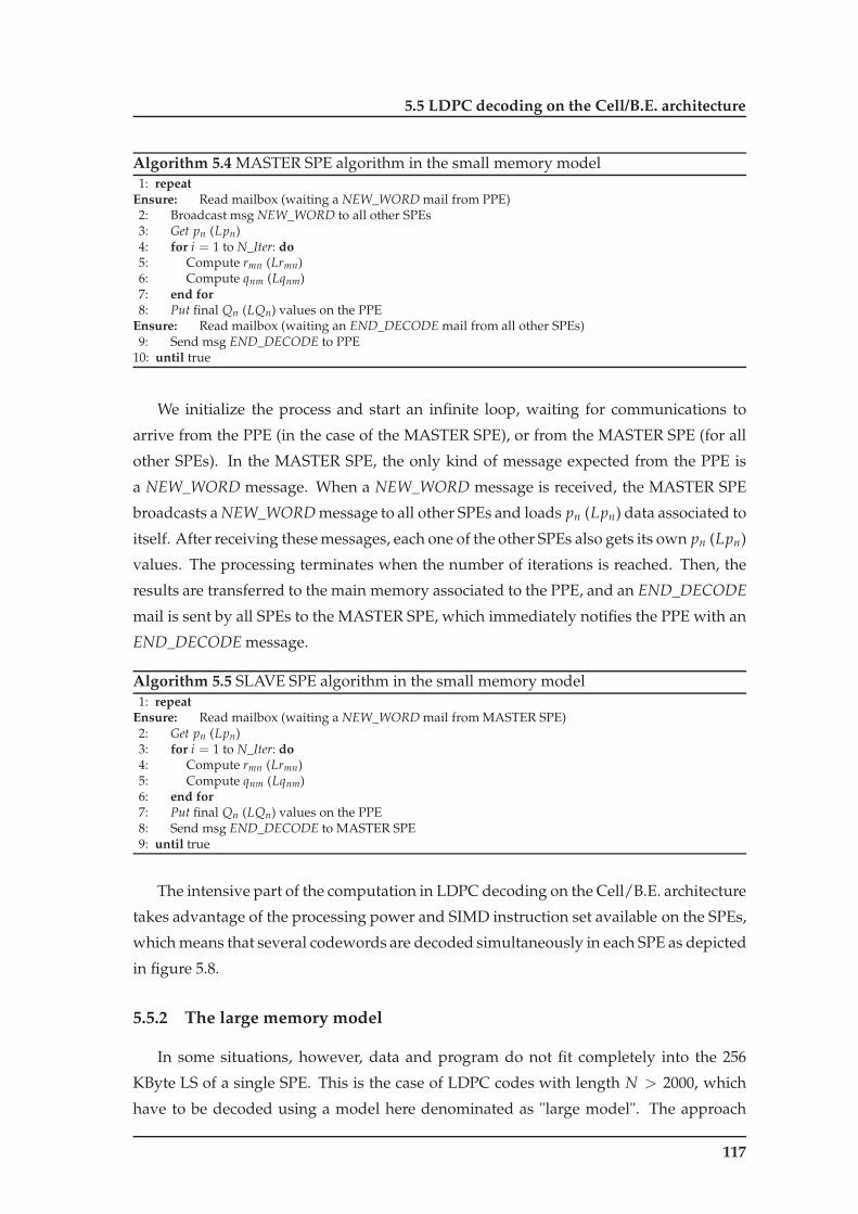
5.5 LDPC decoding on the Cell/B.E. architecture
Algorithm 5.4 MASTER SPE algorithm in the small memory model1: repeat
Ensure: Read mailbox (waiting a NEW_WORD mail from PPE)2: Broadcast msg NEW_WORD to all other SPEs3: Get pn (Lpn)4: for i = 1 to N_Iter: do5: Compute rmn (Lrmn)6: Compute qnm (Lqnm)7: end for8: Put final Qn (LQn) values on the PPE
Ensure: Read mailbox (waiting an END_DECODE mail from all other SPEs)9: Send msg END_DECODE to PPE
10: until true
We initialize the process and start an infinite loop, waiting for communications to
arrive from the PPE (in the case of the MASTER SPE), or from the MASTER SPE (for all
other SPEs). In the MASTER SPE, the only kind of message expected from the PPE is
a NEW_WORD message. When a NEW_WORD message is received, the MASTER SPE
broadcasts a NEW_WORD message to all other SPEs and loads pn (Lpn) data associated to
itself. After receiving these messages, each one of the other SPEs also gets its own pn (Lpn)
values. The processing terminates when the number of iterations is reached. Then, the
results are transferred to the main memory associated to the PPE, and an END_DECODE
mail is sent by all SPEs to the MASTER SPE, which immediately notifies the PPE with an
END_DECODE message.
Algorithm 5.5 SLAVE SPE algorithm in the small memory model1: repeat
Ensure: Read mailbox (waiting a NEW_WORD mail from MASTER SPE)2: Get pn (Lpn)3: for i = 1 to N_Iter: do4: Compute rmn (Lrmn)5: Compute qnm (Lqnm)6: end for7: Put final Qn (LQn) values on the PPE8: Send msg END_DECODE to MASTER SPE9: until true
The intensive part of the computation in LDPC decoding on the Cell/B.E. architecture
takes advantage of the processing power and SIMD instruction set available on the SPEs,
which means that several codewords are decoded simultaneously in each SPE as depicted
in figure 5.8.
5.5.2 The large memory model
In some situations, however, data and program do not fit completely into the 256
KByte LS of a single SPE. This is the case of LDPC codes with length N > 2000, which
have to be decoded using a model here denominated as "large model". The approach
117

5. LDPC decoding on multi- and many-core architectures
followed in this case is described in algorithms 5.6 and 5.7 and consists of having the PPE
control process orchestrating the kernels execution on the SPEs and also data transfers.
The number of data transfers between the PPE and the SPEs is substantially higher in the
large model, because a complete iteration has to be processed sequentially on K partitions
of the Tanner graph. Synchronization is performed through mailboxes.
PPE program: One of the main tasks of the PPE is to execute a waiting loop, listening
for mailbox communications arriving from the SPEs. The Cell/B.E. hardware supports
a dual thread execution mode, where two threads perform the following tasks: one lis-
tens communications from SPEs 0 to N_SPEs/2 − 1 and the other from N_SPEs/2 to
N_SPEs− 1.
Algorithm 5.6 is executed in the PPE. It mainly orchestrates the overall execution
mechanism on the SPEs, as well as data sorting of the buffers to be transmitted to each
SPE. In the main memory several buffers are dedicated to each SPE. They are used to
manage data during the K steps of an iteration of the decoding algorithm. Some of these
buffers are represented in figure 5.10 as Unsorted buffer 1 to Unsorted buffer N_SPEs, and
Sorted buffer 1 to Sorted buffer N_SPEs. These buffers are used to manage the yn data
initially received from the channel at the input of the LDPC decoder, which is processed
to generate pn (Lpn) data that is sent to each SPE. They also represent the place where the
results received from each SPE are accommodated and reorganized. The Unsorted buffers
hold data arriving from each SPE, which is then sorted and placed into Sorted buffers
before being sent again to each SPE to continue the computation of an iteration. The
sorting procedure is depicted in figure 5.10 and it consists of organizing groups of CNs
(or BNs, depending if we are processing, respectively, the horizontal or vertical kernels)
in contiguous data blocks of memory to accelerate DMA transfers. When the buffers
are created, a number of threads equal to the number of SPEs is also created and the
addresses of the different locations to be copied are passed to them. All the buffers to
be transferred by DMA are aligned in memory on a 128-bit boundary and the SPEs use
these addresses to perform DMA data transfers.
On every iteration, two different kinds of actions must be completed K times: i) a
sub-block of the rmn (Lrmn) or qnm (Lqnm) data is sorted and placed in the buffers to be
transmitted to the SPE; and ii) the processed data (BNs or CNs alternately updated) is
sent from the SPE back to the main memory. The actions are synchronized on both sides
of the PPE and SPE. After completing the first action, confirmation mails are sent to
the SPEs, while after concluding the last action, confirmation mails are awaited from the
SPEs. When data is loaded into the buffers in main memory, confirmation mails inform
the SPEs that the DMA transfers can start: for the first sub-block of data to compute, a
118

5.5 LDPC decoding on the Cell/B.E. architecture
DMA data
transfers
LDPC multi-codeword partitioned
decoding based on SIMDI/O, sorting and
data orchestration
L1 DATA CACHE
L1 INSTRUCTION
CACHE
Sorted buffer 1
PPE
MAIN MEMORY
(256MB)
Unsorted buffer 1
Unsorted buffer N_SPEs
SPEMEMD
MA
SPEMEMD
MA
SPEMEMD
MA
SPEMEMD
MA
SPEMEMD
MA
Sorted buffer N_SPEs
Sorting()
Data sorting (pre-processing on the PPE)
Data transfers PPE SPE
(K block data transfers
per iteration)
Figure 5.10: Parallel LDPC decoder on the Cell/B.E. architecture running the large mem-ory model.
NEW_WORD mail is sent to the SPE to make it start loading data from the buffer in main
memory and, when this transfer completes, to initiate the load of the next data buffer.
For the sake of simplicity of representation, the inner loop in algorithm 5.6 omits the
synchronization on the PPE side in steps ranging from 12 to 14, for indicating that old
information present in the SPE buffers has already been replaced and that the PPE needs
to sort a new sub-block with rmn (Lrmn) or qnm (Lqnm) data. Here, the PPE would expect
mails from the SPEs notifying that there is new data available in the Unsorted buffers
waiting to be sorted.
Finally, when all the iterations are completed, the SPEs send END_DECODE messages
to the PPE to conclude the current decoding process and get ready to start processing new
words.
119

5. LDPC decoding on multi- and many-core architectures
Algorithm 5.6 PPE algorithm in the large memory model1: Allocate Sorted buffers and Unsorted buffers2: for th_ctr = 1 to N_SPEs: do3: Create th_ctr thread4: Send Sorted buffers and Unsorted buffers addresses to the thread5: end for6: repeat7: Receives yn from the channel and calculates pn (Lpn)8: Send msg NEW_WORD to all SPEs9: for i = 1 to N_SPEs: do
10: for i = 1 to N_Iter: do11: for block = 1 to K: do12: Get data1 block to SPE[i]13: Put data2 block from SPE[i] /* data1 and data2 will be alternately rmn (Lrmn) and qnm (Lqnm)
*/14: Sorted buffers← Unsorted buffers /* Sort data blocks on the PPE side */15: end for16: end for17: end forEnsure: Wait until mail is received (SPE[i].mailboxcount > 0)18: msg = SPE[i].mailbox (received msg END_DECODE from all SPEs?)19: until msg != END_DECODE
SPE program: In the large model, the SPEs are also dedicated to the computationally
intensive updating of all CNs and BNs by executing sub-blocks of kernel 1 and kernel 2
alternately, during each iteration of the LDPC decoder. The SPE procedure is described
in algorithm 5.7.
The process is initialized and starts an infinite loop, waiting for communications
to arrive from the PPE. At this point, the communication expected from the PPE is a
NEW_WORD message. At first, when a NEW_WORD message is received, the SPE loads
the pn (Lpn) data. After that, the first horizontal sub-block of qnm (Lqnm) data is read into
the buffer on the SPE. As soon as the DMA transfer completes, a new one is immediately
started, so that the next transfer of a vertical sub-block of rmn (Lrmn), or an horizontal
sub-block of qnm (Lqnm), is performed in parallel with the execution of data previously
loaded on the SPE. This way, data transfers are masked by calculations using the double
buffering technique. When a new mail is received, the SPE starts a new computation
to perform either CN or BN updating. When it completes, the SPE updates the buffers
with the new processed data and then starts a new transfer. It should be noticed that
time spent performing communications should balance the computation time, which is
important to achieve efficiency within the architecture.
After completing the processing of a kernel, it waits for the previous DMA transfer
to complete and then performs a new DMA transfer to send processed data back to main
memory. When the transfer is concluded, a confirmation mail is sent to the PPE indicating
that the new data in the Unsorted buffer is available and can be sorted by the PPE in order
to proceed with the following processing. The computation terminates when the number
120
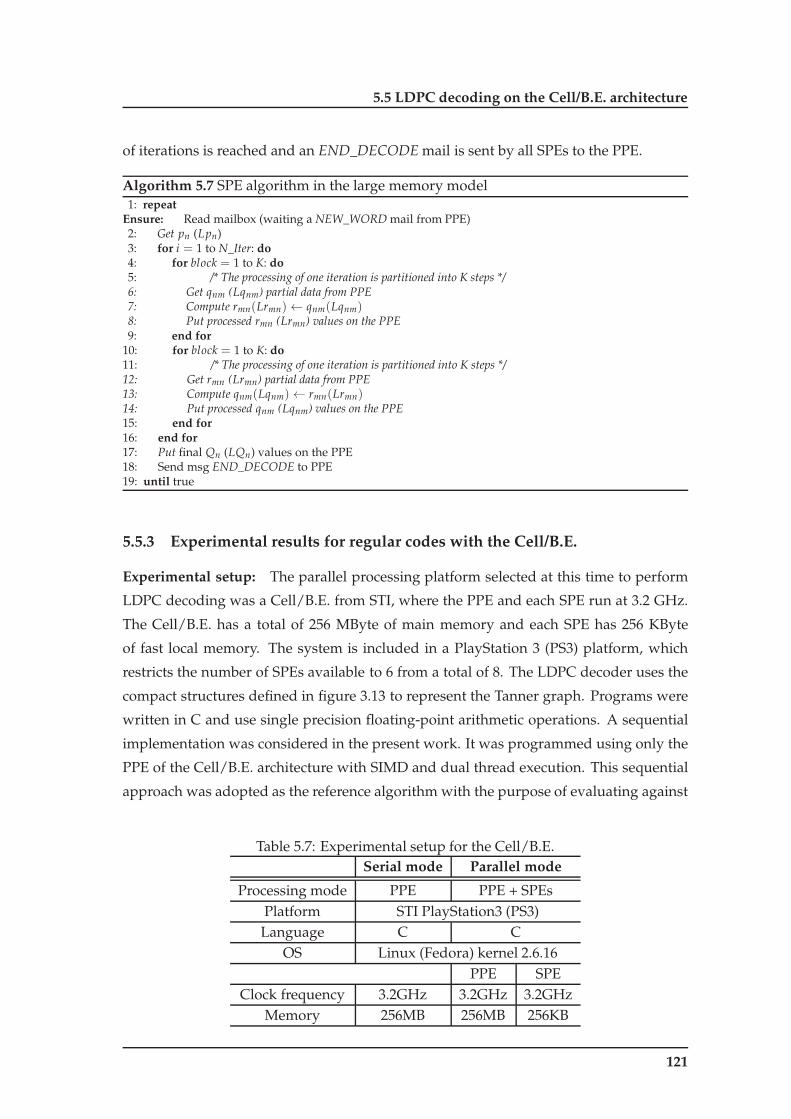
5.5 LDPC decoding on the Cell/B.E. architecture
of iterations is reached and an END_DECODE mail is sent by all SPEs to the PPE.
Algorithm 5.7 SPE algorithm in the large memory model1: repeat
Ensure: Read mailbox (waiting a NEW_WORD mail from PPE)2: Get pn (Lpn)3: for i = 1 to N_Iter: do4: for block = 1 to K: do5: /* The processing of one iteration is partitioned into K steps */6: Get qnm (Lqnm) partial data from PPE7: Compute rmn(Lrmn)← qnm(Lqnm)8: Put processed rmn (Lrmn) values on the PPE9: end for
10: for block = 1 to K: do11: /* The processing of one iteration is partitioned into K steps */12: Get rmn (Lrmn) partial data from PPE13: Compute qnm(Lqnm)← rmn(Lrmn)14: Put processed qnm (Lqnm) values on the PPE15: end for16: end for17: Put final Qn (LQn) values on the PPE18: Send msg END_DECODE to PPE19: until true
5.5.3 Experimental results for regular codes with the Cell/B.E.
Experimental setup: The parallel processing platform selected at this time to perform
LDPC decoding was a Cell/B.E. from STI, where the PPE and each SPE run at 3.2 GHz.
The Cell/B.E. has a total of 256 MByte of main memory and each SPE has 256 KByte
of fast local memory. The system is included in a PlayStation 3 (PS3) platform, which
restricts the number of SPEs available to 6 from a total of 8. The LDPC decoder uses the
compact structures defined in figure 3.13 to represent the Tanner graph. Programs were
written in C and use single precision floating-point arithmetic operations. A sequential
implementation was considered in the present work. It was programmed using only the
PPE of the Cell/B.E. architecture with SIMD and dual thread execution. This sequential
approach was adopted as the reference algorithm with the purpose of evaluating against
Table 5.7: Experimental setup for the Cell/B.E.Serial mode Parallel mode
Processing mode PPE PPE + SPEsPlatform STI PlayStation3 (PS3)
Language C COS Linux (Fedora) kernel 2.6.16
PPE SPEClock frequency 3.2GHz 3.2GHz 3.2GHz
Memory 256MB 256MB 256KB
121

5. LDPC decoding on multi- and many-core architectures
Table 5.8: Parity-check matrices H under test for the Cell/B.E.Matrix Size Edges Edges/row Edges/col.)
(M× N) (wc ×M) (wc) (wb)
p1 128× 256 768 {6} {3}p2 252× 504 1512 {6} {3}p3 512× 1024 3072 {6} {3}p4 2448× 4896 14688 {6} {3}p5 288× 576 1824 {2,3,6} {6,7}p6 480× 576 – {2,3,4} {20}p7 560× 672 – {2,3,4} {20}p8 480× 960 – {2,3,6} {6,7}p9 800× 960 3200 {2,3,4} {20}
p10 576× 1152 – {2,3,6} {6,7}p11 960× 1152 – {2,3,4} {20}p12 624× 1248 3952 {2,3,6} {6,7}p13 1040× 1248 – {2,3,4} {20}
parallel solutions. The experimental setup is depicted in table 5.7, and matrices under
test are presented in table 5.8.
To evaluate the performance of the proposed stream-based LDPC decoder, the Cell/B.E.
was programmed using both small and large models. In the small model, a complete ma-
trix fits the SPE LS memory and the processing is efficiently completed using few data
transactions between the PPE and the SPEs. In the large model, the decoding of a code-
word is performed by decomposing the Tanner graph (i.e., the rmn (Lrmn), qnm (Lqnm) and
corresponding data structures) into different sub-blocks and applying the SPE to process
them on a sequential basis. Matrices for LDPC codes p1 to p3 and p5 to p7 fit into the
LS of a single SPE and were programmed using the small model, while matrix p4 is too
large to fit into a single SPE and has to be processed on a sub-block by sub-block basis,
using the large model described in subsection 5.5.2. Matrix p3 was also implemented
in the large model to allow a comparison between the two computational models. All
processing times were obtained for decoders performing a number of iterations ranging
from 10 to 50.
Experimental results with the small model: Figure 5.11 presents the decoding times
for matrices p1 to p3 under the small model running the SPA. They relate the execution
time needed for the Cell/B.E. to decode a codeword with the processing time required
to decode a codeword on the sequential version. The Cell/B.E. performs concurrent pro-
cessing on the 6 SPEs, each using SIMD to process 4 codewords simultaneously. The
decoding time for matrix p3 shows that the Cell/B.E. takes approximately 353.6µs to de-
122

5.5 LDPC decoding on the Cell/B.E. architecture
Table 5.9: Decoding throughputs for a Cell/B.E. programming environment in the smallmodel running the SPA with regular LDPC codes (Mbps)
Number of iterations Matrix p1 Matrix p2 Matrix p3
10 68.5 69.1 69.525 28.0 28.3 28.450 14.2 14.2 14.3
Data structures size (KByte) 35.8 70.6 143.4
code 24× 1024-bit codewords on the 6 SPEs (an average value of 14.7µs per codeword)
in 10 iterations, against 244.9µs per codeword on the serial version that concurrently de-
codes 8 codewords (dual thread decoding using SIMD) for the same number of iterations.
It achieves a throughput of 69.5 Mbps which compares well against VLSI LDPC decoders.
Observing table 5.9, we conclude that the decoding capacity per bit is high and approxi-
mately constant for all the regular codes under test (matrices p1, p2 and p3). Comparing
this throughput with that obtained on the serial approach, the speedup achieved with
the Cell/B.E. surpasses 16. In the serial mode, the PPE accesses the main memory that is
slower than the LS on the SPEs which, as a consequence, has an influence on the reported
speedup [38].
Experimental evaluation also shows that regarding the same algorithm applied only
to one SPE, decoding 4 codewords, the full version that uses 6 SPEs decoding 24 code-
words, achieves a speedup only 14% below the maximum (6), or equivalently an effi-
p1 p2 p3 p1 p2 p3 p1 p2 p30
0.2
0.4
0.6
0.8
1
1.2
1.4
H matrix
Dec
odin
g tim
e (m
s)
ParallelSerial
10 it.10 it.
10 it.
25 it.
25 it.
25 it.
50 it.
50 it.
50 it.
Figure 5.11: LDPC decoding times per codeword for sequential and parallel modes onthe Cell/B.E., running the SPA with regular codes in the small model (ms)
123

5. LDPC decoding on multi- and many-core architectures
ciency E f = 86%. In fact, the number of data transfers is low in this model, which
means that the overhead in communications introduced by using a higher number of
SPEs would be marginal. This allows to conclude that the solution is scalable under the
small memory model.
Experimental results with the large model: In this case, the 256 KByte of LS memory
in the SPE are not enough to fit the complete data structures necessary to decode 4 code-
words and also the program. The maximum regular code allowed is limited by the LS
size, and for a rate = 1/2 code it can be described according to (wc represents Edges per
row and N the codeword size):
N × wb × 36 + 32× N + Program_Size ≤ 256KByte. (5.1)
The processing is then performed in successive partitions of the Tanner graph and the
number of data transfers and synchronization operations degrades the performance of
the decoder. In the large model a single iteration has to be performed using several
data transactions. Data transfers between each SPE and the main memory become the
most significant part of the global processing time. Also, the intensive sorting procedure
performed by the PPE and the large number of data transactions involve concurrent ac-
cesses to the slow main memory that can cause some processors to temporarily idle in
this model. This is the main reason why the throughput decreases significantly in this
model. Matrix p3 was also tested in the large model to allow relatively assessing the two
computational models, and the reported throughput running the SPA for 10 iterations,
decreases to 9 Mbps which represents a throughput more than 7 times lower than the one
obtained using the small model. Matrices with lengths equivalent or superior to p4 are
too large to fit into a single SPE and have to be processed on a sub-block by sub-block ba-
sis, using the large model. They all achieve throughputs inferior to 9 Mbps, which led to
the conclusion that the Cell/B.E. processor is not efficient for LDPC decoding with large
H matrices.
Increasing the number of SPEs used in the architecture would cause the throughput
to rise, but not by the same percentage as in the small model. This is explained by the fact
that the use of more SPEs further increases data communications and the effect of data
sorting, which clearly become the bottleneck in the large model.
Analyzing the performance on the Cell/B.E.: The N_SPEs number of SPEs available
and the number of instructions per iteration Nop/iter have a major impact in the over-
all performance of the decoder on the Cell/B.E. This performance also depends on the
number of iterations Niter and frequency of operation fop. Here, the throughput perfor-
mance (T) can be estimated for the small model according to (5.2). Differently from what
124

5.5 LDPC decoding on the Cell/B.E. architecture
10 25 50 1000
2
4
6
8
10
12
14
16
18
Niter
Dec
odin
g tim
e (m
s)
Lower bound (optimal case)Real value (measured)Upper bound (worst case condition)
Figure 5.12: Model bounds for execution times obtained on the Cell/B.E.
happens in other parallel architectures, where a task is responsible for decoding only a
part of the Tanner graph, in this approach and processing model each SPE performs the
complete processing of the Tanner graph as described in algorithms 2.1 and 2.2, indepen-
dently from the other SPEs. The LDPC decoder supports peak data transfers between the
SPE and main memory of approximately 4GByte/s [2] and, consequently, its performance
is mainly limited by the number of SPEs that are simultaneously trying to access the main
memory. Tppe→spe and Tspe→ppe represent data transfer times between PPE and SPE.
T =N_SPEs× 4× N
Tppe→spe +Nop/iter×Niter
fop+ Tspe→ppe
[bps]. (5.2)
The proposed LDPC decoder suits scalability, and it could be easily adopted by other gen-
erations of this family of processors having a higher number of SPEs available. In that
case, it would be able to decode more codewords simultaneously, increasing even more
the speedup and throughput of the decoder. The model proposed in (5.2) makes it dificult
to predict the execution time, not because the number of instructions Nop/iter generated
by the Cell SDK 2.1 compiler is unknown, but rather due to the parallel pipeline that per-
forms data transfers independently from arithmetic operations and whose behavior can-
not be predicted due to branch misprediction penalties that force emptying the pipeline.
Nevertheless, the model can be used to establish the limits of performance. We decided to
adopt upper and lower bounds representing processing times, respectively, for worst and
best case working conditions. The worst case condition (upper bound) assumes process-
125

5. LDPC decoding on multi- and many-core architectures
ing and memory accesses are performed without any level of parallelism and a branch
misprediction occurs after every instruction (a very unrealistic condition). The best case
condition (lower bound) assumes that no branch mispredictions occur and that there is
full parallelism (overlap) between memory accesses and computation. Figure 5.12 shows
that the parallelism supported by the dual-pipelined Cell/B.E. architecture exploits the
LDPC decoder near the optimal case. The measured experimental results are only 6%
worst than those estimated for the best case working conditions, here defined by the
lower bound, and the algorithm executes very close to the maximum performance the
Cell/B.E. can provide. Measured values and lower bounds almost overlap in figure 5.12.
5.5.4 Experimental results for irregular codes with the Cell/B.E.
To increase the efficiency of the LDPC decoder we implemented the MSA on the
Cell/B.E.. It requires less computation, based essentially in addition and comparison
operations. Additionally, we also adopted the Forward-and-Backward simplification of
the algorithm [83] that avoids redundant computation and eliminates repeated accesses to
memory. In the MSA, data elements have 8-bit integer precision, which allows packing
16 data elements per 128-bit memory access. This increases the arithmetic intensity of the
algorithm, which favors the global performance of the LDPC decoder. The instruction
set of the Cell/B.E. architecture supports intrinsic instructions to deal efficiently with
these parallel 128-bit data types. Moreover, because there are 6 SPEs available, in this
implementation the algorithm supports the simultaneous decoding of 96 codewords in
parallel. However, the set of 8-bit integer intrinsic parallel instructions of the Cell/B.E. is
more limited than those of the 32-bit floating-point family of instructions. This explains
that the speedup obtained when changing from the SPA to the MSA is lower than we
would expect.
Running LDPC WiMAX codes on the Cell/B.E.: Table 5.10 shows the throughputs ob-
tained decoding a subset of WiMAX IEEE 802.16e standard [64] irregular codes, consid-
ering 10 iterations. A more vast set of results can be found in [33]. In some cases they
approach quite well, while in others they even surpass the 75 Mbps required by the stan-
dard to work in (theoretical) worst case conditions. For the two codes with N = 576
represented by matrices p5 and p6, when running 10 iterations we obtain throughputs
of 79.8 and 79.3 Mbps. For codes p12 and p13, with N = 1248 and for the same number
of iterations, they range from 79.6 to 78.4 Mbps. All codes in table 5.10 were tested for
the MSA and approach quite well the maximum theoretical limit of 75 Mbps. They all
show better performances than those obtained with the SPA. Furthermore, if we consider
a lower number of iterations, the decoder’s throughputs may rise significantly. For ex-
126

5.6 LDPC decoding on GPU-based architectures
Table 5.10: Decoding throughputs for a Cell/B.E. programming environment in the smallmodel running the MSA with irregular WiMAX LDPC codes (Mbps)
Number of iterations p5 p6 p7 p8 p9 p10 p11 p12 p13
10 79.8 79.3 78.5 79.6 78.4 79.6 78.4 79.6 78.425 32.7 32.5 32.2 32.6 32.1 32.6 32.1 32.6 32.150 16.5 16.4 16.2 16.4 16.2 16.4 16.2 16.4 16.2
ample, for 5 iterations instead of 10, the throughput is approximately the double (above
145 Mbps).
5.6 LDPC decoding on GPU-based architectures§
Following an alternative parallel approach, the design of software LDPC decoders
on GPUs is proposed in the next sections. The algorithms were implemented by us-
ing the programming interfaces presented in the previous sections, namely the CUDA
from NVIDIA [97] and the Caravela [125], which are nowadays massively disseminated
and provide efficient tools to exploit low-cost computational power and achieve flexi-
bility/reprogrammability for LDPC decoding.
The development of flow-models to perform LDPC decoding and apply them to
GPUs under the context of Caravela hadn’t been tried before. It was the first time that
this type of complex and irregular LDPC decoding algorithms were parallelized and ac-
celerated in the scope of this thesis [40,41]. Under this context, Caravela flow-models were
developed to perform LDPC decoding based on the SPA to test the viability of the so-
lution with a demanding computational workload. Although it hasn’t been tested, ap-
plying the MSA (computationally less demanding) to GPUs using the Caravela is also
possible using a similar approach. In the CUDA context, we also proposed to investi-
§Some portions of this section appear in:
[32] Falcão, G., Silva, V., Gomes, M., and Sousa, L. (2008). Edge Stream Oriented LDPC Decoding. In Pro-ceedings of the 16th Euromicro International Conference on Parallel, Distributed and network-based Processing(PDP’08), pages 237–244, Toulouse, France.
[34] Falcão, G., Silva, V., and Sousa, L. (2009b). How GPUs can outperform ASICs for fast LDPC decod-ing. In Proceedings of the 23rd ACM International Conference on Supercomputing (ICS’09), pages 390–399.ACM.
[37] Falcão, G., Sousa, L., and Silva, V. (2008). Massive Parallel LDPC Decoding on GPU. In Proceedings ofthe 13th ACM SIGPLAN Symposium on Principles and practice of parallel programming (PPoPP’08), pages83–90, Salt Lake City, Utah, USA. ACM.
[40] Falcão, G., Yamagiwa, S., Silva, V., and Sousa, L. (2007). Stream-Based LDPC Decoding on GPUs. InProceedings of the First Workshop on General Purpose Processing on Graphics Processing Units – GPGPU’07,pages 1–7.
[41] Falcão, G., Yamagiwa, S., Silva, V., and Sousa, L. (2009d). Parallel LDPC Decoding on GPUs using aStream-based Computing Approach. Journal of Computer Science and Technology, 24(5):913–924.
[39] Falcão, G., Sousa, L., and Silva, V. (accepted in February 2010b). Massively LDPC Decoding on Mul-ticore Architectures. IEEE Transactions on Parallel and Distributed Systems.
127

5. LDPC decoding on multi- and many-core architectures
gate SPA and MSA-based LDPC decoders for regular codes, and MSA-based decoders
for irregular LDPC codes, namely those applied to the DVB-S2 standard.
5.6.1 LDPC decoding on the Caravela platform
Under the Caravela context, the pixel processors are the only programmable proces-
sors and the processing is based on square 2D textures, with dimensions power of 2,
as depicted in figure 5.13. As shown in the same figure, the Caravela’s computational
model is based on a bijective application between pixel processors and pixel textures,
which means that there is only one entry point for each pixel processor. This character-
istic poses difficult challenges in the development of kernels 1 and 2 of algorithm 2.1.
Under this context, the processing of each individual edge is associated to a single pixel
processor. For each pixel processor to be able of accessing several data elements from
a unique entry point, we developed a circular addressing mechanism dedicated to Car-
avela that suits well the irregular data accesses imposed by the algorithm, as described
next.
T1
T2
T3
T4
T5
T6
T7
T8
T9
T10
T11
T12
T13
T14
T15
T16
Pixel
Processors
Pixel
TexturesP13 entry point
P1
P2
P3
P4
P5
P6
P7
P8
P9
P10
P11
P12
P13
P14
P15
P16
Figure 5.13: 2D textures Tn associated to pixel processors Pn in Caravela.
The tenths of pixel processors available allow exposing parallelism, but impose a type
of processing based on textures, where each pixel texture represents an edge of the Tanner
graph. This solution imposes redundant computation because it does not allow the re-
utilization of data. Nevertheless, the level of parallelism achieved is consistent [40,41] and
the approach effectively allowed to develop parallel LDPC decoding algorithms based
on the simultaneous update of several BNs or CNs processed by distinct pixel processors
(following an edge approach, where each pixel processor only updates an edge). In order
to implement such an approach, dedicated data structures were developed to support
the texture based processing of the SPA (described in algorithm 2.1).
Stream-based data structures for the Caravela: To take advantage of the processing
performance of GPUs, efficient data structures adapted for 2D textures and for stream
128

5.6 LDPC decoding on GPU-based architectures
computing were derived from those presented in section 3.3.3. A stream-based LDPC
decoder needs different computation and memory access patterns when executing con-
secutive kernels to update BNs and CNs, respectively. In order to support the execution
of kernels 1 and 2 (see figure 5.7) on the GPU based on the Caravela platform, we propose
two stream-based data structures adapted from HBN and HCN presented in section 3.3.3.
These data structures are suitable for stream computing both regular and irregular LDPC
codes on the GPU grid based on 2D textures with dimensions that are a power of 2. Al-
gorithm 5.8 details this procedure for the case of HBN , depicted in figure 5.14 for the H
matrix shown in figure 2.1. In step 5, it can be seen that all edges associated with the same
CN are collected and stored in consecutive positions inside HBN . The addressing in each
row of H becomes circular. The pixel element corresponding to the last non-null element
Algorithm 5.8 Generating compact 2D HBN textures from original H matrix1: /* Reading a binary M× N matrix H */2: for all CNm (rows in Hmn) : do3: for all BNn (columns in Hmn) : do4: if Hmn == 1 then5: ptrnext = j : Hmj == 1, with n + 1 ≤ j < (n + N) mod N;
/* Finding circularly the right neighbor on the current row */6: HBN = ptrnext;
/* Store ptrnext into the HBN structure, using a square texture of dimension 2D × 2D , with
D =
⌈
12 × log2(
M∑
m=1
N∑
n=1Hmn)
⌉
*/
7: end if8: end for9: end for
of each row points to the first element of this row, implementing a circular addressing
that is used to update all associated messages in that row. The circular addressing allows
to introduce a high level of parallelism. In the limit, for a multi-processor platform, a
different pixel processor can be allocated to every single edge, i.e. to the computation
of each individual message. Each element of the data structure, here represented by a
pixel texture, records the address of the next entry pointer and the corresponding value
of rmn. Although the pixel elements in figure 5.14 are represented by their row and col-
umn addresses, the structures can be easily vectorized by convenient 1D or 2D reshaping
according to the target stream-based architecture they apply to. The 3D representation
in figure 5.14 shows that the same matrix information can be used to simultaneously de-
code several codewords (multi-codeword decoding), by applying SIMD processing, for
example.
In the upper left corner of figure 5.14, it can be seen that the pixel processor allo-
cated to compute the message miCN0→BN0
(identified as message r0,0) depends on mes-
sages mi−1BN1→CN0
and mi−1BN2→CN0
coming from BN1 and BN2. This is equivalent to saying
that to update BN0 (upper left pixel), we have to read the information from BN1 (BN0
129
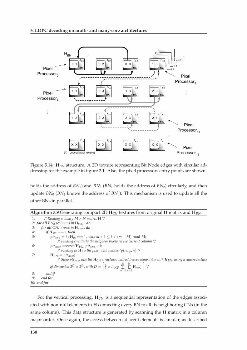
5. LDPC decoding on multi- and many-core architectures
word 2
HBN
word 1
r0,0
r0,1
r0,2
r1,3
r1,4
r1,5
r2,0
r2,3
r2,6
r3,1
r3,4
r3,7
2 1
rx,x
X X
rx,x
X X
rx,x
X X
rx,x
X X
….
(X = unused pixel texture)
….
word n
….
2 2 2 3 1 2
1 1 0 3 1 3 2 0
BN0
0 1 0 2 0 0 1 0BN
1BN
2
….
BN3
BN4
BN5
BN0
BN3
BN6
BN1
BN4
BN7
Pixel
Processor0
Pixel
Processor4
Pixel
Processor15
Pixel
Processor3
….
Pixel
Processor11
….
Figure 5.14: HBN structure. A 2D texture representing Bit Node edges with circular ad-dressing for the example in figure 2.1. Also, the pixel processors entry points are shown.
holds the address of BN1) and BN2 (BN1 holds the address of BN2) circularly, and then
update BN0 (BN2 knows the address of BN0). This mechanism is used to update all the
other BNs in parallel.
Algorithm 5.9 Generating compact 2D HCN textures from original H matrix and HBN
1: /* Reading a binary M× N matrix H */2: for all BNn (columns in Hmn) : do3: for all CNm (rows in Hmn) : do4: if Hmn == 1 then5: ptrtmp = i : Hin == 1, with m + 1 ≤ i < (m + M) mod M;
/* Finding circularly the neighbor below on the current column */6: ptrnext =search(HBN, ptrtmp, n);
/* Finding in HBN the pixel with indices (ptrtmp, n) */7: HCN = ptrnext;
/* Store ptrnext into the HCN structure, with addresses compatible with HBN , using a square texture
of dimension 2D × 2D , with D =
⌈
12 × log2(
M∑
m=1
N∑
n=1Hmn)
⌉
*/
8: end if9: end for
10: end for
For the vertical processing, HCN is a sequential representation of the edges associ-
ated with non-null elements in H connecting every BN to all its neighboring CNs (in the
same column). This data structure is generated by scanning the H matrix in a column
major order. Once again, the access between adjacent elements is circular, as described
130

5.6 LDPC decoding on GPU-based architectures
(Single 1 in column 6)
(Single 1 in column 5)
(Single 1 in column 2)
HCN
word 1
word 2
q0,0
q0,1
q0,2
q1,3
q1,4
q1,5
q2,0
q2,3
q2,6
q3,1
q3,4
q3,7
qx,x
X X
qx,x
X X
qx,x
X X
qx,x
X X
….
(X = unused pixel texture)
(Single 1 in column 7)
….
….
word n
CN0
CN2
CN0
CN3
CN1
CN2
CN1
CN3
….
1 2 2 1 -1 -1 1 3
2 2 -1 -1 0 0 0 3
-1 -1 0 1 1 0 -1 -1
Pixel
Processor0
Pixel
Processor4
….
Pixel
Processor15
Pixel
Processor3
….
Pixel
Processor11
Figure 5.15: HCN structure. A 2D texture representing Check Node edges with circu-lar addressing for the example in figure 2.1. Also, the pixel processors entry points areshown.
in algorithm 5.9 and illustrated in figure 5.15 for the H matrix given in figure 2.1. In
this case, a careful construction of the 2D addresses in HCN is required, because every
pixel texture representing a graph edge must be in exactly the same position as it is in
HBN. This meticulous positioning of the pixel elements in HCN allows the processing to
be performed alternately for both kernels, using the same input textures. Step 6 shows
that ptrnext is placed in the same pixel texture (or n, m edge) that it occupies in HBN.
Figure 5.15 describes how the HCN data structure is organized for the same example in
figure 2.1, under kernel 2. The message miBN0→CN0
(identified as message q0,0) is a function
of p0, mi−1CN2→BN0
and should update the upper left pixel representing CN0, which holds
the address of CN2. This is another way of saying that CN2 updates CN0, and vice-versa.
This mechanism works in the same way for all the other CNs in the grid.
LDPC decoders on the Caravela platform: We developed a flow-model to support the
LDPC decoder based on Caravela tools, which uses efficient mechanisms provided for re-
cursive computation [129]. The SDF graph in figure 5.7 represents the stream-based LDPC
decoder and figure 5.16 graphically describes the corresponding flow-model unit con-
taining a shader program that supports the stream-based computation of kernels 1 and 2,
where the input and output data streams are 2D textures. In the first iteration, the input
data stream 0 represents data channel probabilities. The first output stream is produced
131

5. LDPC decoding on multi- and many-core architectures
Input Data Stream 3
Constant Values
Output Data Stream 0
BNs Update OR
Shader Program
H CN .x
H CN
.y
X
weight
Input Data Stream 2 H
BN .x
H BN
.y
X
weight
Flow-model
Input Data Stream 0 q
0_3
q 0_2
q 0_1
q 0_0
r (i-1)_3 |q (i-1)_3
r (i-1)_2
|q (i-1)_2
r (i-1)_1 |q (i-1)_1
r (i-1)_0 |q (i-1)_0
q i_3
q i_2
q i_1
q i_0
Input Data Stream 1
p 0_3
p 0_2
p 0_1
p 0_0
1st iter.?
CNs Update
Figure 5.16: Organization of the LDPC decoder flow-model.
by performing kernel 1. After the first execution, this stream directly feeds the input of
the next flow-model unit that executes kernel 2. Data streams can be multiplexed through
a simple and efficient swapping mechanism [129]. The output data stream can be feedback
as an input stream of the next flow-model unit execution, and the process is repeated for
each iteration. Also, the input H matrix is placed into an input stream and kernel 1 and
kernel 2 are processed in pixel processors, according to figures 5.14, 5.15 and 5.16. At the
end, the last output stream conveys the decoded codeword.
5.6.2 Experimental results with Caravela
Experimental setup: The proposed algorithm was programmed in recent GPUs and its
performance is analyzed for different workloads (i.e. H matrices with distinct character-
istics). The experimental setup is presented in table 5.11. It includes an 8800 GTX GPU
from NVIDIA, with stream processors (SPs) running at 1.35 GHz. The used GPU sup-
ports single precision floating-point arithmetic. The LDPC decoders are programmed on
the GPU using version 2.0 of the OpenGL Shading Language and the Caravela library.
The experiments were carried out by using five matrices of different sizes and with vary-
ing number of edges, matrices c1 to c5 in table 5.12. Their properties were chosen to
132

5.6 LDPC decoding on GPU-based architectures
Table 5.11: Experimental setup for CaravelaGPU
Platform NVIDIA 8800 GTXClock frequency 1.35 GHz (SP)
Memory 768 MBLanguage OpenGL (GLSL)
Table 5.12: Parity-check matrices H under test for CaravelaMatrix Size Edges Edges/row Texture Dim. Unused pixel textures8
c1 111× 999 2997 {27} 64× 64 1099c2 408× 816 4080 {10} 64× 64 16c3 212× 1908 7632 {36} 128× 128 8752c4 2448× 4896 14688 {6} 128× 128 1696c5 2000× 4000 16000 {8} 128× 128 384
simulate a full set of computational workloads with code sizes typically ranging from
small to medium and large (all sizes covered), and approximately similar to those used
in recent communication standards. The pixel processors of the GPU were used with
data inputted as textures and the output data stream assuming the usual place of the
pixel color components’ output in a graphical application. However, all programming
details are hidden from the programmer by using the Caravela interface tool.
Experimental results programming the flow-model on the GPU using Caravela: The
experimental results in figure 5.17 show the processing times obtained to decode the
LDPC codes from table 5.12. The performance of the GPU increases as the intensity
of processing also increases, but not necessarily just depending on it. Comparing ma-
trix c1 with matrix c2, it can be shown that even though the latter has fewer unused
pixel textures that represent no edges in the Tanner graph, the former has a better ratio
decoding time/Edge executing 25 iterations. Although matrix c1 has more edges per row
than c2 (27 against 10), GPUs perform better for algorithms demanding intensive com-
putation and small amount of data communications. Experimental results in figure 5.17
show that the GPU performs better for large matrices. Although matrix c5 has a number
of edges almost four times superior to c2, and even with a similar number of edges per
row (8 against 10), the ratio decoding time/Edge is favorable in matrix c5. It performs
more than two times better than the latter (3µs against 7.3µs).
The GPU-based approach shows better results for the LDPC decoding algorithm with
8These are the pixels showing empty coordinates (x, x) in figures 5.14 and 5.15, imposed by the GPUCaravela interface that only supports 2D data textures with square dimensions D× D, where D is a powerof 2.
133

5. LDPC decoding on multi- and many-core architectures
c1
c2
c3
c4
c5
0
50
100
150
200
250
Matrix
LDPC Decoding Time (ms)
25 iterations
50 iterations
100 iterations
Figure 5.17: Decoding times running the SPA on an 8800 GTX GPU from NVIDIA pro-grammed with Caravela.
intensive computation on huge quantities of data, due to parallelism features and pro-
cessing power.
5.6.3 LDPC decoding on CUDA-based platforms
A different approach consists of exploiting a many-core system with a programming
model based on multi-threads, as the one supported by the NVIDIA Tesla series’ GPUs
using the CUDA [80]. Differently from previous GPU families which could only program
pixel processors, the CUDA provides a more efficient exploitation of the computational
resources of a GPU. Here, geometry, pixel and vertex programs share common stream
processing resources, and the GPUs used in this new approach are based on this unified
architecture (CUDA).
In order to achieve LDPC decoding supported by CUDA, algorithms 2.1 and 2.2 were
applied to these parallel programmable devices as described next. The initial approach
followed on CUDA-based GPUs was similar to the one described previously under the
Caravela context in section 5.6.1. The processing adopted was also based on a thread-
per-edge approach [32,37]. This solution presents the same penalties as those mentioned in
section 5.6.1, because it does not use the efficient forward-and-backward method that al-
low data reutilization and save memory accesses. Furthermore, the algorithms presented
in [32,37] are based on the SPA. Better results are achieved using the more efficient MSA,
134

5.6 LDPC decoding on GPU-based architectures
that only has to perform add and compare operations. To overcome these difficulties we
adopted a different approach based on a thread-per-node approach (thread-per-CN and
thread-per-BN based processing) [34].
Algorithm 5.10 GPU algorithm (host side)1: Allocate buffers in the host and buffers on device (cudamalloc)2: Read HBN and HCN data structures (edges’ addresses) from file to the host buffers3: Send HBN and HCN data structures to buffers on the GPU device4: Configure the grid on device (number of blocks and number of threads per block)5: repeat6: Receives yn from the channel and calculate pn (Lpn)7: Send pn (Lpn) data to buffers on the GPU device8: for i = 1 to N_Iter: do9: Launch kernel 1 (horizontal processing) for the calculation of rmn (Lrmn) data on the GPU
10: Launch kernel 2 (vertical processing) for the calculation of qnm (Lqnm) data on the GPU11: end for12: Transfer final Qn (LQn) values to the host13: until true
Multi-thread based programming on the CUDA: Unlike the Caravela solution, the
CUDA-based approach recovers data structures HBN and HCN originally presented in
subsection 3.3.3. Algorithm 5.10 illustrates how processing is performed in this approach.
In the beginning of a new processing, after the necessary data buffers are allocated both
on host and device, data to be computed (HBN, HCN, rmn (Lrmn) and qnm (Lqnm) data struc-
tures) is distributed over a predefined number of blocks on the grid of multi-threads.
Each block contains tx × ty elements that represent threads. Threads are grouped in
warps and dispatched by one of the 128 stream processors according to the thread-per-
CN or thread-per-BN structure of the algorithm and the thread scheduler, as mentioned
before. In the horizontal processing step, each thread updates all the BNs associated to
a CN (an entire row of H). Rather than moving data from global to fast (but complex)
shared memory, an equally efficient processing strategy can be achieved by moving data
directly to the registers of the core. The number of registers available per multiproces-
sor on the GPU is high enough to accommodate the input data and corresponding data
structures. Increasing the number of threads per block often allows hiding latency and
achieving better performance, as long as we guarantee that there are enough registers
per thread on the GPU to compile. For every different application we need to estimate
the best fitting number of threads per block. The minimum consists of 64, but 128 or 256
threads per block can be used until a maximum of 512. Figure 5.18 depicts the internal
processing inside a block, where the update of every BN message represented by rmn
(Lrmn) is calculated according to the structure previously identified in HBN.
A similar principle applies to the update of qnm (Lqnm) messages, or vertical process-
ing. Here, each thread updates all the CNs associated to a BN (an entire column of H).
135

5. LDPC decoding on multi- and many-core architectures
r0,0
r0,1
r0,2 CN
0
r2,0
r2,3
r2,6 CN
2
r1,3
r1,4
r1,5 CN
1
tx
ty
thread j
thread u
thread v
Figure 5.18: Detail of tx× ty threads executing on the GPU grid inside a block for kernel 1(the example refers to figure 3.12 and shows BNs associated to CN0, CN1 and CN2 beingupdated).
Coalesced memory accesses: In the 8 series’ GPU from NVIDIA the global memory is
not cached. The latency can be up to 400-600 cycles and is likely to become a performance
bottleneck. One way to turn around this problem and increase performance significantly
consists in using coalescence. Instead of performing 16 individual memory accesses, all
the 16 threads of a half-warp (maximum fine-grain level of parallelism on the G80x fam-
ily) can access the global memory of the GPU in a single coalesced read or write access.
But the elements have to lie on a contiguous memory block, where the kth thread accesses
the kth data element, and data and addresses must obey, respectively, to specific size and
alignment requirements [34]. Figure 5.19 shows the activity of half-warps 0 and 1 captured
at two different instants, where 16 threads (t0 to t15) read data in a single coalesced mem-
ory transaction from the GPU’s slow global memory. However, HBN, HCN, rmn (Lrmn)
and qnm (Lqnm) data structures have to be properly disposed in a contiguous mode (from
a thread perspective) in order to allow the coalesced accesses to be performed in a sin-
gle operation. This data realignment action is stated in Proposition 1 and depicted in
figure 5.19 which shows the simultaneous access of groups of 16 threads to memory.
Proposition 1. For decoding regular LDPC codes using the proposed stream-based data
structures shown in figure 3.12, it is possible to compute each kernel of algorithms 2.1
and 2.2 using full coalesced memory accesses for either read or write operations, but not for
both.
Proposition 1 is fulfilled by applying the following transformations to the data struc-
tures. Equations (5.3) to (5.6) represent the permutations necessary for kernel 1, where:
newAddr = j ∗ p + k div wc + (k mod wc) ∗ 16, (5.3)
136
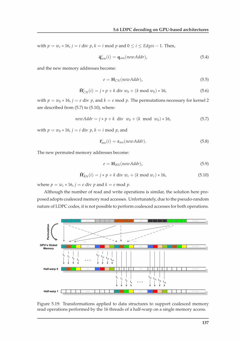
5.6 LDPC decoding on GPU-based architectures
with p = wc ∗ 16, j = i div p, k = i mod p and 0 ≤ i ≤ Edges− 1. Then,
qcnm(i) = qnm(newAddr), (5.4)
and the new memory addresses become:
e = HCN(newAddr), (5.5)
HcCN(i) = j ∗ p + k div wb + (k mod wb) ∗ 16, (5.6)
with p = wb ∗ 16, j = e div p, and k = e mod p. The permutations necessary for kernel 2
are described from (5.7) to (5.10), where:
newAddr = j ∗ p + k div wb + (k mod wb) ∗ 16, (5.7)
with p = wb ∗ 16, j = i div p, k = i mod p, and
rcmn(i) = rmn(newAddr). (5.8)
The new permuted memory addresses become:
e = HBN(newAddr), (5.9)
HcBN(i) = j ∗ p + k div wc + (k mod wc) ∗ 16, (5.10)
where p = wc ∗ 16, j = e div p and k = e mod p.
Although the number of read and write operations is similar, the solution here pro-
posed adopts coalesced memory read accesses. Unfortunately, due to the pseudo-random
nature of LDPC codes, it is not possible to perform coalesced accesses for both operations.
... ... ......
... ... ......
... ... ......
t3
Half-warp 0
Half-warp 1
t0 t
1 t2
... ... ......
... ...
t15
t12 t
13 t14
t3
t0 t
1 t2
GPU’s Global
Memory
Permutation
t12 t
13 t14 t
15
Figure 5.19: Transformations applied to data structures to support coalesced memoryread operations performed by the 16 threads of a half-warp on a single memory access.
137
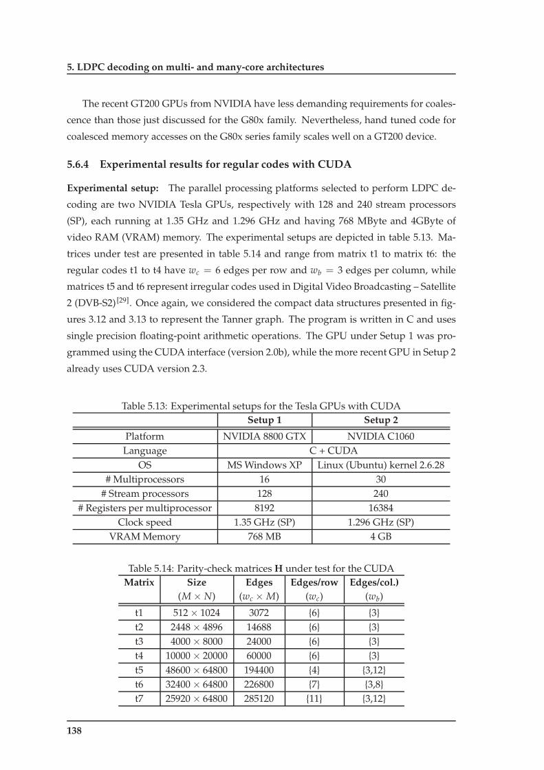
5. LDPC decoding on multi- and many-core architectures
The recent GT200 GPUs from NVIDIA have less demanding requirements for coales-
cence than those just discussed for the G80x family. Nevertheless, hand tuned code for
coalesced memory accesses on the G80x series family scales well on a GT200 device.
5.6.4 Experimental results for regular codes with CUDA
Experimental setup: The parallel processing platforms selected to perform LDPC de-
coding are two NVIDIA Tesla GPUs, respectively with 128 and 240 stream processors
(SP), each running at 1.35 GHz and 1.296 GHz and having 768 MByte and 4GByte of
video RAM (VRAM) memory. The experimental setups are depicted in table 5.13. Ma-
trices under test are presented in table 5.14 and range from matrix t1 to matrix t6: the
regular codes t1 to t4 have wc = 6 edges per row and wb = 3 edges per column, while
matrices t5 and t6 represent irregular codes used in Digital Video Broadcasting – Satellite
2 (DVB-S2) [29]. Once again, we considered the compact data structures presented in fig-
ures 3.12 and 3.13 to represent the Tanner graph. The program is written in C and uses
single precision floating-point arithmetic operations. The GPU under Setup 1 was pro-
grammed using the CUDA interface (version 2.0b), while the more recent GPU in Setup 2
already uses CUDA version 2.3.
Table 5.13: Experimental setups for the Tesla GPUs with CUDASetup 1 Setup 2
Platform NVIDIA 8800 GTX NVIDIA C1060Language C + CUDA
OS MS Windows XP Linux (Ubuntu) kernel 2.6.28# Multiprocessors 16 30
# Stream processors 128 240# Registers per multiprocessor 8192 16384
Clock speed 1.35 GHz (SP) 1.296 GHz (SP)VRAM Memory 768 MB 4 GB
Table 5.14: Parity-check matrices H under test for the CUDAMatrix Size Edges Edges/row Edges/col.)
(M× N) (wc ×M) (wc) (wb)
t1 512× 1024 3072 {6} {3}t2 2448× 4896 14688 {6} {3}t3 4000× 8000 24000 {6} {3}t4 10000× 20000 60000 {6} {3}t5 48600× 64800 194400 {4} {3,12}t6 32400× 64800 226800 {7} {3,8}t7 25920× 64800 285120 {11} {3,12}
138

5.6 LDPC decoding on GPU-based architectures
Experimental results on the GPU using CUDA: All regular matrices under test were
run for Setup 1, on blocks with a varying number of threads ranging from 64 to 128. Only
the best results achieved are reported in tables 5.15 and 5.16. Matrix t1 was programmed
to use 16 blocks of the grid and 64 threads per block. Using more threads per block would
have been possible, but it would decrease the number of simultaneous active blocks to
a value below 16 which would cause the 16 multiprocessors not to be fully occupied,
reducing parallelism and performance. Matrix t2 occupies 128 threads per block and 39
blocks. Matrix t3 uses 63 blocks and 128 threads per block and matrix t4 157 blocks and
also 128 threads per block. The higher level of parallelism expectedly supported by the
next GPU generations, advises the use of at least 100 blocks in order to exploit full poten-
tial and make the solution scalable to future devices with more stream processors. In this
case, the number of blocks used is imposed by the size of the LDPC code. At the same
time it also depends on the number of threads per block, which in the LDPC decoder for
Setup 1 are limited to 128 due to the high number of registers used per multiprocessor.
Table 5.15 presents the overall measured decoding throughputs running the SPA on
an 8800 GTX GPU from NVIDIA, considering 32 and 8-bit precision data elements. Ex-
perimental results in the table show that the GPU-based solution can be faster than the
Cell/B.E.-based one for LDPC codes with dimensions above matrix t1. The GPU-based
implementation shows significantly higher throughputs for intensive computation on
large quantities of data. A throughput above 18.3 Mbps is achieved for matrix t3 with
24000 edges and executing 10 iterations, while it decreases to 11.3 Mbps for significantly
larger codes (60000 edges and above). In the latter, the size of the data structures to rep-
Table 5.15: LDPC decoding throughputs for a CUDA programming environment runningthe SPA with regular codes (Mbps)
Number of iterations Matrix t1 Matrix t2 Matrix t3 Matrix t432-bit 8-bit 32-bit 8-bit 32-bit 8-bit 32-it 8-bit
10 10.0 14.6 17.9 31.9 18.3 40.4 11.3 40.125 5.3 6.5 10.1 14.6 10.0 18.9 5.1 18.150 2.4 3.3 5.9 7.7 5.7 10.1 2.7 9.5
resent the matrix is so large that they do not fit into the 64 KByte of constant memory
used in smaller codes (t3 and below), which degrades the performance because con-
stant memory on the GPU uses a different bus from global memory. For small codes
and with a small number of iterations, better results are achieved with fewer threads
per block, although the decoding time differences are minimal if we vary the number
of threads per block. However, when decoding larger codes with a higher number of
iterations, the reported speedups are higher when a larger number of threads per block
139

5. LDPC decoding on multi- and many-core architectures
is used. Figure 5.20 shows the importance of memory accesses in the overall processing
t1 t2 t3 t40
10
20
30
40
50
60
70
80
90
100
Matrix H
Thr
ead
exec
utio
n tim
e (%
)
Reading data from memoryReading indices from memory
Writing data to memoryRemaining processing
Figure 5.20: Thread execution times for LDPC decoding on the GPU running the SPA.
time as the size of the LDPC code increases. Reports obtained for matrices t1 to t4 run-
ning on the GPU show that the time spent in coalesced memory reads is approximately
constant (in percentage) for all matrices, while the more expensive and often conflicting
non-coalesced memory write operations can represent a bottleneck after a certain dimen-
sion of the LDPC code. Figure 5.20 shows that because we use coalescence to read data,
if the number of edges changes, the percentage of the overall processing time remains
approximately constant at around 20%. For matrix t4 (60000 edges), non-coalesced write
accesses occupy nearly 50% of the total processing time, against 39% for matrix t3 (24000
edges), and only 24% in matrix t1 (3072 edges). This shows that using coalescence as
described in Proposition 1, is extremely important not only because parallel accesses to
memory can be performed by multiple threads concurrently, but also because the number
of data collisions decreases.
Data precision that best fits the arithmetic intensity on the GPU: We also tested the
LDPC decoder for the SPA using data with only 8-bit precision, instead of the original
32-bit precision, which allowed us to pack 16 elements into 128-bit data elements. In
this case, using the 8-bit precision solution, the throughputs obtained for 10 iterations in
matrices t1 to t4 range from 14.6 up to 40.1 Mbps. The reason for this improvement is
mainly related with the reduction of memory accesses performed per arithmetic opera-
tion. On the GPU side, data is unpacked and processed, causing one memory access to
140

5.6 LDPC decoding on GPU-based architectures
Table 5.16: LDPC decoding times on the GPU (ms) and corresponding throughputs(Mbps) for an 8-bit data precision solution decoding 16 codewords in parallel runningthe MSA with regular codes.
Time (ms) Throughput (Mbps)Number of iterations 10 20 30 50 10 20 30 50
Matrix t1 0.393 0.597 0.765 1.102 41.7 27.4 21.4 14.9Matrix t3 1.331 1.589 1.812 2.261 96.2 80.6 70.6 56.6Matrix t4 2.932 3.176 3.425 3.841 109.1 100.8 93.4 83.3
read/write 16 elements at a time. Even considering the increase in arithmetic operations,
the GPU still performs faster. The limitation in performance is imposed mainly by mem-
ory accesses. The highest throughputs are achieved for matrices t3 and t4, which provide
results superior to 40 Mbps. Due to the use of the efficient forward and backward al-
gorithm [83] that minimizes the number of memory accesses and also the number of add
and multiply operations, the experimental results here reported are much superior to the
ones obtained in [37].
Another approach based on CUDA exploits the MSA. The results achieved with the
MSA are reported in table 5.16 and are superior to those obtained with the SPA. The ma-
trices under test are t1, t3 and t4. As referred before, matrix t1 uses 64 threads per block
and a total of 16 blocks. Matrices t3 and t4 use 128 threads per block and 63 and 157
blocks, respectively. The decoding times reported in table 5.16 define global processing
times, which include data transfers according to the denominator of (5.12), to simulta-
neously decode 16 codewords with length depending on the matrix. Data elements are
represented and processed using 8-bit precision, causing 16 data elements to be read in
each 128-bit memory access. The GPU seems to perform better for larger codes. If we
consider throughput, it is interesting to see that the GPU achieves a higher coded data
rate for matrix t4, which has 60000 edges to compute. In this case, a very significant
throughput of 109.1 Mbps is achieved running 10 iterations. It decodes 16 codewords
simultaneously, each of length 20000-bit, in 2.932 ms.
Analyzing the performance on the GPU with CUDA: A model to predict the through-
put T of the parallel LDPC decoder on the GPU is presented in (5.12), where Th denotes
the total number of threads running on the GPU, MP the number of multiprocessors and
SP the corresponding number of stream processors per multiprocessor. Each thread is
expected to access memory with latency L per memory access, with a total of Mop mem-
ory accesses. NDop/iter represents the number of cycles for non-divergent instructions
performed per iteration within a kernel, while Dop/iter represents divergent instructions.
Finally, Niter defines the number of iterations, N is the size of the codeword, and fop the
141

5. LDPC decoding on multi- and many-core architectures
frequency of operation of a stream processor. The processing Tproc time is:
Tproc = Niter
ThMP × (
NDop/iter
SP + Dop/iter) + Th×Mop× L
fop. (5.11)
Then, the global throughput can be obtained by:
T =P× N
Thost→gpu + Tproc + Tgpu→host[bps], (5.12)
where P defines the parallelism (number of codewords being simultaneously decoded).
Thost→gpu and Tgpu→host represent data transfer times between host and device.
The model defined in (5.11) can be further detailed in order to allow the prediction
of numerical bounds that can help describing the computational behavior of the LDPC
decoder on the CUDA. One iteration executes kernel 1 and kernel 2, while memory ac-
cesses can be decomposed into coalesced and non-coalesced read and write operations,
each one imposing different workloads. The CUDA Visual Profiler tool was used in or-
der to obtain the number of instructions and memory accesses per kernel. Considering
for example the code for matrix t4, which has a workload large enough to fully occupy
157 blocks of the grid with a maximum of 128 threads per block (#Th = 157× 128), an
average number of cycles per kernel (excluding load and store operations) similar in both
kernels and equal to NDop/iter = 3867, and having less than 0.5% of divergent threads
which allow us to approximate Dop/iter ≈ 0, (5.11) can be rewritten as:
Tproc =2Niter ×
ThMP ×
NDop/iter
SP
fop+
Th×Mop× Lfop
︸ ︷︷ ︸
TMemAccess
. (5.13)
TMemAccess defines all memory access operations and can be decomposed in memory ac-
cesses to CNs and BNs, respectively:
TMemAccess = TMemAccBNs + TMemAccCNs. (5.14)
TMemAccBNs defines time spent doing memory access to update CNs (accessing BNs):
TMemAccBNs = NiterM× wc × L + M× 2wc × L/16
fop, (5.15)
and TMemAccCNs represents the time necessary to update BNs (accessing CNs):
TMemAccCNs = NiterN × wb × L + N × (2wb + 1)× L/16
fop. (5.16)
The last partials in (5.15) and (5.16) show memory read operations, which are divided
by 16 to model the parallelism obtained with the introduction of coalesced reading op-
erations. In spite of the latency L can be up to 400-600 cycles, we believe that the thread
142

5.6 LDPC decoding on GPU-based architectures
scheduler operates very efficiently, producing effectively faster memory accesses. Ap-
parently, the scheduler is good enough maintaining the cores occupied and hiding the
memory latency. For code t4 our model predicts the processing time quite well, with an
error inferior to 13% assuming L = 4. Transferring data structures between host and
device at a bandwidth of 1.2 GB/s (an experimentally measured value) represents an
increase in 8.9% on the global processing time.
5.6.5 Experimental results for irregular codes with CUDA
The number of edges of LDPC codes used, for example, in DVB-S2 assumes signifi-
cant proportions, as depicted from table 2.3. For every iteration, the number of messages
to be updated is twice the value shown in field #Edges. For example, when running 10
iterations of the decoder for code t7, which has rate = 3/5, a total of 2× 285120 × 10 =
5702400 > 5.7M messages have to be processed in a short period of time in order to guar-
antee minimum acceptable throughput. Until very recently, such performances were only
possible to achieve using dedicated VLSI, as it is the case of the hardware solution pro-
posed in chapter 4 of this thesis. However, considering the high processing power and
bandwidth of GPUs, in this chapter we show that with these programmable devices it is
possible to achieve performances similar to those obtained with VLSI hardware.
Running LDPC DVB-S2 codes on the GPU with CUDA: Codes t5, t6 and t7 from ta-
ble 5.14 are a subset of DVB-S2 codes. They represent long length irregular codes with
maximal and minimal number of edges (see table 2.3 in chapter 2) used in the standard,
and for these reasons were selected to be decoded on a platform based on Setup 2, which
has more multiprocessors available than Setup 1. They represent, respectively, B1, B4 and
B5 irregular LDPC codes which can be found in annexes B and C of the standard [29]. Al-
though Setup 2 has more registers per multiprocessor than Setup 1, the number of threads
allowed per block still has limitations. In this case, the LDPC decoder is limited to 256
threads per block due to the high number of registers that each kernel uses per multipro-
cessor. The GPU from Setup 2 has 240 stream processors and 30 multiprocessors and the
horizontal and vertical kernels demand less than 76 registers per thread. In this case this
is acceptable because the C1060 GPU allows to use up until 16384 registers per multipro-
cessor as shown in table 5.13, and the quantity of threads used per block keep the total
number of registers bellow that value. Each block of the GPU was tested with a varying
number of threads ranging from 64 to 256, and the best results were achieved with 128
threads per block for codes t5 and t6, while 192 threads per block produce better results
for code t7. As for the solutions based on Setup 1, so does the number of blocks used here
is imposed by the size of the LDPC code and number of threads per block adopted. Ma-
143

5. LDPC decoding on multi- and many-core architectures
Table 5.17: LDPC decoding times on the GPU (ms) and corresponding throughputs(Mbps) for an 8-bit data precision solution decoding 16 codewords in parallel runningthe MSA with irregular DVB-S2 codes.
Matrix Iter. Thost→gpu + Tgpu→host (ms) Tproc (ms) Throughput (Mbps)
t5
1
3.1
1.99 205.72 3.97 147.65 9.90 80.1
10 19.85 45.320 39.66 24.350 99.00 10.2
t6
1
3.4
2.30 180.72 4.58 129.45 11.40 69.9
10 22.85 39.420 45.72 21.150 114.12 8.8
t7
1
4.1
3.87 129.72 7.68 88.05 19.20 44.5
10 38.5 24.320 76.72 12.850 192.09 5.3
trices t5 and t6 were programmed to use 507 blocks of the grid, while matrix t7 occupies
338 blocks. Table 5.17 presents the decoding times and throughputs obtained running the
MSA on a C1060 GPU (described in Setup 2, table 5.13). Experimental results reported
in the table show that the GPU-based solution here proposed supports the intensive pro-
cessing of LDPC codes with very high dimensions within acceptable decoding times. By
executing 1 iteration of the decoder for matrix t5 (which has 194400 edges), the solution
achieves a processing time of 1.99 ms and a throughput of 205.7 Mbps, which respectively
change to 19.85 ms and 45.3 Mbps when executing 10 iterations. The increase in process-
ing time is not linear because for small Tproc processing times, Thost→gpu + Tgpu→host data
transfer times still have a significant weight in the overall processing time. Matrix t6 has
a higher number of edges (226800), which allows obtaining 180.7 Mbps executing 1 it-
eration and 39.9 Mbps for 10 iterations. Matrix t7 represents the DVB-S2 code with the
highest number of edges (285120) and in this case throughput decreases to 129.7 Mbps
for 1 iteration and to 24.3 Mbps executing 10 iterations of the algorithm.
Additionally, this programmable solution proposed for GPUs also considers different
data representations, namely by using 8 or 16-bit precision. Table 5.18 presents through-
puts for both cases running code t6, where the 8-bit solution decodes 16 codewords in
144
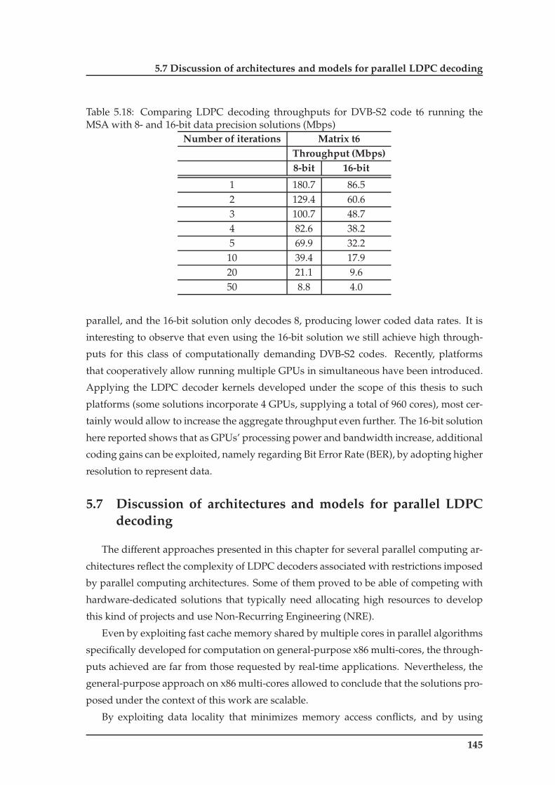
5.7 Discussion of architectures and models for parallel LDPC decoding
Table 5.18: Comparing LDPC decoding throughputs for DVB-S2 code t6 running theMSA with 8- and 16-bit data precision solutions (Mbps)
Number of iterations Matrix t6Throughput (Mbps)8-bit 16-bit
1 180.7 86.52 129.4 60.63 100.7 48.74 82.6 38.25 69.9 32.2
10 39.4 17.920 21.1 9.650 8.8 4.0
parallel, and the 16-bit solution only decodes 8, producing lower coded data rates. It is
interesting to observe that even using the 16-bit solution we still achieve high through-
puts for this class of computationally demanding DVB-S2 codes. Recently, platforms
that cooperatively allow running multiple GPUs in simultaneous have been introduced.
Applying the LDPC decoder kernels developed under the scope of this thesis to such
platforms (some solutions incorporate 4 GPUs, supplying a total of 960 cores), most cer-
tainly would allow to increase the aggregate throughput even further. The 16-bit solution
here reported shows that as GPUs’ processing power and bandwidth increase, additional
coding gains can be exploited, namely regarding Bit Error Rate (BER), by adopting higher
resolution to represent data.
5.7 Discussion of architectures and models for parallel LDPCdecoding
The different approaches presented in this chapter for several parallel computing ar-
chitectures reflect the complexity of LDPC decoders associated with restrictions imposed
by parallel computing architectures. Some of them proved to be able of competing with
hardware-dedicated solutions that typically need allocating high resources to develop
this kind of projects and use Non-Recurring Engineering (NRE).
Even by exploiting fast cache memory shared by multiple cores in parallel algorithms
specifically developed for computation on general-purpose x86 multi-cores, the through-
puts achieved are far from those requested by real-time applications. Nevertheless, the
general-purpose approach on x86 multi-cores allowed to conclude that the solutions pro-
posed under the context of this work are scalable.
By exploiting data locality that minimizes memory access conflicts, and by using
145

5. LDPC decoding on multi- and many-core architectures
Table 5.19: Comparison with state-of-the-art ASIC LDPC decoders using the MSA.Rate Code length Precision Iterations Throughput
(K/N) (N) (bits) (Mbps)[108] 5/6 2304 8 10 30.4[81] 1/2 2304 6 20 63
[111] 1/2 2304 8 8 60Matrix t3 1/2 8000 8 10 96.2
[GPU proposed solution]
several SPE cores that support SIMD and a dual pipelined architecture, the Cell/B.E.
achieves throughputs between 70 and 80 Mbps for small to medium LDPC codes. The
limitation in performance for larger codes is imposed by the size of the LS memory on
the SPEs. The adoption of specific parallelization techniques for the Cell/B.E. platform
here described produced throughputs that approach well hardware solutions [81,108]. For
the SPA, it nearly achieves 70 Mbps [38] running 10 iterations of the algorithm. Moreover,
we also implemented LDPC decoders based on the MSA for the Cell/B.E., using codes
adopted in the WiMAX standard (IEEE 802.16e) [64], which have lengths inferior to 2304
bits. We achieved throughputs near 80 Mbps running 10 iterations [33,36] of the decoder,
which approaches throughputs that until recently were only achievable using dedicated
hardware (e.g. VLSI). Furthermore, this solution can provide a lower BER regarding
VLSI-based architectures.
GPUs, which are shared memory based multiprocessors, can also be programmed
with Caravela and CUDA. The former is a general, while the latter is an efficient pro-
gramming framework developed for NVIDIA devices. These GPUs are more efficient
than Cell/B.E. for LDPC decoding medium and large length codes. We tested a vast
set of codes where we included LDPC codes used in the DVB-S2 standard and report
throughputs ranging from dozens of Mbps to over 100 Mbps, depending on the length
of the code or number of multiprocessors of the GPU adopted. Here, the constraints
are imposed by bandwidth limitations between host and device, and also by conflicting
memory accesses to the global memory of the GPU, which can be minimized by using
coalesced read/write operations that significantly improve the performance of the algo-
rithm. The adoption of specific parallelization strategies for the GPU platform here de-
scribed, produced throughputs that approach well hardware-based solutions. Table 5.19
presents some comparisons with recently published work. The throughputs obtained
compare well with those reported in recent publications [17,81,108,111] that describe dedi-
cated hardware solutions (ASIC and others) to implement LDPC decoders.
Figure 3.3 shows that the average number of iterations depends on the Signal-to-
146

5.8 Summary
Noise Ratio (SNR) of input data, which naturally influences the decoding time. It can be
seen that the 8-bit precision solution here developed for the CUDA compares favorably
in terms of the number of iterations needed for the algorithm to converge. Again, as in
the case of Cell/B.E.-based LDPC decoders, this programmable solution also presents
superior performance in terms of BER, when compared with ASIC architectures that use
5 to 6-bit precision to represent data.
5.8 Summary
Changes in technical computing now provide massive computational power at low-
cost. The advent of high-value graphics computing offers the possibility of increased pro-
ductivity and flexibility on a variety of intensive algorithms used in real-time demanding
applications.
This chapter presents the most relevant results obtained for LDPC decoding on multi-
and many-core platforms. These platforms can be divided into three distinct classes:
general-purpose multi-cores based on the x86 shared memory architecture; the Cell/B.E.
from the STI consortium which is based on a distributed memory model; and GPUs, also
based on a shared memory model and here exploited under the Caravela and CUDA con-
texts. They allow exposing distinct parallel properties of an LDPC code. We developed
LDPC decoding algorithms and data structures appropriate for parallel computing. They
are used to measure the performance under these parallel computing platforms. The dis-
similarities between the architectures and the comparison of performances are presented
in this chapter. We conclude that some of them offer performances that approach well
hardware-dedicated (e. g. VLSI) solutions. We also present in this chapter models that
try to estimate their behavior under controlled parameters. These estimates allow to
conclude that both architectures can be programmed to work very close from their peak
performance.
147

5. LDPC decoding on multi- and many-core architectures
148

We shall not cease from explorationAnd the end of all our exploring
Will be to arrive where we startedAnd know the place for the first time.
T.S. Eliot, in "Four Quartets"


6Closure
Contents6.1 Future work . . . . . . . . . . . . . . . . . . . . . . . . . . . . . . . . . . . 154
151

6. Closure
Due to the computationally intensive nature of Low-Density Parity-Check (LDPC)
decoders, hardware approaches have been developed over the last years. They mainly
use Very Large Scale Integration (VLSI) technology, which is able to efficiently handle the
complex processing required by LDPC decoding in order to provide high throughputs.
The purposes of the research work developed under the scope of this thesis were
threefold. The first consisted of developing and optimizing VLSI parallel LDPC decoder
systems with a reduced number of processors. The second objective was to investigate
new paradigms, parallel algorithms and suitable stream-based data structures able of
performing LDPC decoding efficiently. The third and last purpose of this research was
to derive parallel kernels for a set of predefined multi-core architectures and assess their
performance against state-of-the-art VLSI solutions.
In this thesis it has been shown that such hardware solutions for LDPC decoding can
be implemented with a reduced number of processors supported by a minor reconfigura-
tion of the memory blocks of the system. Using a small number of processors significantly
simplifies the routing complexity of the design, allowing savings in terms of area, devel-
opment costs and complexity. Small process design technologies used in Application
Specific Integrated Circuits (ASIC) (90nm and below) allow to operate this architecture
at frequencies high enough to guarantee throughputs able of supporting the demanding
Digital Video Broadcasting – Satellite 2 (DVB-S2) requirements. The smallest area result
achieved in this work is approximately 7 mm2. This research has also been conducted to
Field Programmable Gate Array (FPGA) based solutions that are equally able of provid-
ing real-time processing for the same requirements, and led to the following publications:
[31] Falcão, G., Gomes, M., Gonçalves, J., Faia, P., and Silva, V. (2006). HDL Library of Process-
ing Units for an Automatic LDPC Decoder Design. In Proceedings of the IEEE Ph.D. Research
in Microelectronics and Electronics (PRIME’06), pages 349–352.
[51] Gomes, M., Falcão, G., Silva, V., Ferreira, V., Sengo, A., and Falcão, M. (2007b). Flexible
Parallel Architecture for DVB-S2 LDPC Decoders. In Proceedings of the IEEE Global Telecom-
munications Conf. (GLOBECOM’07), pages 3265–3269.
While dedicated hardware still imposes some restrictions, the advent of the multi-
core era encouraged the development of flexible and programmable approaches towards
the computation of LDPC decoding. Presently, a set of parallel architectures exist that
are worldwide disseminated and generally available at low-cost. The Cell Broadband
Engine (Cell/B.E.) architecture suits ideally the decoding of codes with small to medium
lengths, while Graphics Processing Units (GPU) can be used more efficiently for medium
to large length codes. Parallel algorithms were proposed for performing LDPC decoding
by exploiting data parallelism and task parallelism. The results herein reported show that
152

the former can be used to decode efficiently WiMAX LDPC codes achieving throughputs
near 80 Mbps, while the latter can be adopted to decode larger codes, namely those used
in the DVB-S2 standard. Both support decoding either regular or irregular codes. This
work was presented internationally in journals and conferences:
[36] Falcão, G., Silva, V., Sousa, L., and Marinho, J. (2008). High coded data rate and multicode-
word WiMAX LDPC decoding on the Cell/BE. Electronics Letters, 44(24):1415–1417.
[38] Falcão, G., Sousa, L., and Silva, V. (2009c). Parallel LDPC Decoding on the Cell/B.E. Pro-
cessor. In Proceedings of the 4th International Conference on High Performance and Embedded
Architectures and Compilers (HiPEAC’09), volume 5409 of Lecture Notes in Computer Science,
pages 389–403. Springer.
GPUs can be used under different contexts and by using different programming tools.
They can use the Caravela interface, a generic tool for programming kernels on GPUs,
which allows the programmer to use any GPU existing on the market, as reported in the
following journal paper:
[41] Falcão, G., Yamagiwa, S., Silva, V., and Sousa, L. (2009d). Parallel LDPC Decoding on GPUs
using a Stream-based Computing Approach. Journal of Computer Science and Technology,
24(5):913–924.
Or, to achieve superior performance and lower execution times, GPUs from NVIDIA can
also be programmed using the Compute Unified Device Architecture (CUDA) interface,
which supports kernels running under a multi-threaded environment with multiple lev-
els of efficient memory hierarchy. This part of the work performed with CUDA produced
throughputs in the order of hundreds of Mbps and has been presented in some of the best
conferences in the area:
[37] Falcão, G., Sousa, L., and Silva, V. (2008). Massive Parallel LDPC Decoding on GPU. In
Proceedings of the 13th ACM SIGPLAN Symposium on Principles and practice of parallel pro-
gramming (PPoPP’08), pages 83–90, Salt Lake City, Utah, USA. ACM.
[34] Falcão, G., Silva, V., and Sousa, L. (2009b). How GPUs can outperform ASICs for fast
LDPC decoding. In Proceedings of the 23rd ACM International Conference on Supercomputing
(ICS’09), pages 390–399. ACM.
Also, power consumption plays an important role in nowadays autonomous systems.
The more efficient is the exploitation of the parallel computational resources, the better
the ratio Watt-per-bit-decoded can be, which implies that the number of codewords de-
coded in parallel should be the highest. However, to achieve high aggregate throughput,
the execution on GPUs can impose significant latency, which may become unacceptable
153

6. Closure
for some communications. However, other important areas of research can adopt GPUs
as convenient solutions for the intensive problem of LDPC decoding. One example is
related with the study and simulation of new LDPC codes and error floors in the range
of 10−11 to 10−12 (or even further), which typically is not adequate to be achieved by us-
ing dedicated hardware (e.g. VLSI), because it demands flexibility and programmability.
This type of research is based on the massive simulation of LDPC codes and it can be
efficiently achieved on programmable processors such as GPUs, which can accelerate the
computation on CPUs. The GPU-based solutions also support floating-point arithmetic,
which can introduce advantages in terms of Bit Error Rate (BER) regarding to VLSI ap-
proaches:
[39] Falcão, G., Sousa, L., and Silva, V. (accepted in February 2010b). Massively LDPC Decoding
on Multicore Architectures. IEEE Transactions on Parallel and Distributed Systems.
Furthermore, by developing models that try to estimate the behavior of these architec-
tures, we also show that if programmed according to specific and appropriate strategies
targeting high levels of parallelism, LDPC decoding algorithms can perform very close
to the theoretical maximum performance of those architectures. The assessment of their
performances, namely BER and throughput, shows that they can be competitive with
VLSI hardware.
The impact of the research work developed under the scope of this thesis can be mea-
sured not only by the publications that arose from it but also from the high number of
citations to this very recent work. Recently, a chapter has been accepted for publication
at the GPU Computing Gems from NVIDIA, and the source code has been made publicly
available at the gpucomputing.net website:
[35] Falcão, G., Silva, V., and Sousa, L. (2010a). GPU Computing Gems, chapter Parallel LDPC
Decoding. ed. Wen-mei Hwu, vol. 1, NVIDIA, Morgan Kaufmann, Elsevier.
This allows other researchers/engineers to continue this work. By making the source
code publicly available, people with practical interests in LDPC decoders can develop
their own systems and research. Another purpose of this strategy aims at encourag-
ing the scientific/engineering community to develop other types of parallel algorithms,
namely by applying adequate strategies inspired in this work for obtaining high levels of
parallelism able of producing more efficient and faster programs.
6.1 Future work
Although all optimizations performed in the VLSI architecture proposed in chapter 4
of this thesis, there is still room for improvement. Using smaller technologies in the pro-
cess design, such as 65, 45, or even 32 nm, can minimize area and power consumption.
154

6.1 Future work
Taking advantage of higher frequencies of operation (possible with the use of smaller
process technologies) and with a significantly higher effort, deeper changes can be intro-
duced into the architecture by grouping more memories into common blocks of higher
and thinner RAMs, using a more complex time multiplexing strategy. As described in
chapter 4, this can lead to considerable area improvements. Additional improvements
can also be projected to the near future by exploiting the use of memristors, a recent
technology of HP that is expected to revolutionize the manufacturing of RAM memories,
namely by introducing important changes in area and volatility constraints.
CUDA has been proposed to perform LDPC decoding under the context of this the-
sis, but another Application Programming Interface (API) has recently emerged with the
arrival of OpenCL [55], and consequently it should be exploited. OpenCL allows writing
parallel programs once for execution across several heterogeneous platforms that include
CPUs, GPUs and other types of processors (in practice, OpenCL code has minor change
requirements as we move the execution from platform to platform).
Another area potentially exploitable consists of using GPU clusters for the massive
processing of LDPC decoding essentially based on data-parallelism. Here, the main chal-
lenges should be imposed by the shared use of the bus for communications with the host
system. In fact, preliminary tests showed that when performing such iterative computa-
tions in multi-GPU systems, the communication time dominates.
Finally, the utilization of heterogeneous systems that may incorporate, for example,
CPUs, GPUs and FPGAs to cooperatively compute LDPC decoding can also be consid-
ered. Expectedly, it may allow obtaining interesting results, if we successfully try to
overcome the limitations of an architecture with the facilities provided by another.
It should be noticed that, although the work here reported was mainly devoted to the
study of computational models and development of a novel concept for LDPC decoding
based on newly proposed parallel algorithms, it can be applied in the development of
improved and faster algorithms that support other types of computationally demanding
applications. Examples are inference calculation algorithms, such as those used in Turbo
codes, stereo vision applied to robotics, or in Bayesian networks just to name a few. The
methods and solutions proposed in this thesis show that the use of distinct forms of
parallelism to deal with the intensive nature of these computational problems appears to
be tractable.
155

6. Closure
156

Appendices
157

158

AFactorizable LDPC Decoder
Architecture for DVB-S2
ContentsA.1 M parallel processing units . . . . . . . . . . . . . . . . . . . . . . . . . . 160
A.1.1 Memory mapping and shuffling mechanism . . . . . . . . . . . . 161
A.2 Decoding decomposition by a factor of M . . . . . . . . . . . . . . . . . 162
A.2.1 Memory mapping and shuffling mechanism . . . . . . . . . . . . 163
159
A. Factorizable LDPC Decoder Architecture for DVB-S2
The architecture here described surpasses some limitations of [70], and adds flexibility
and easy reconfiguration, according with the decoder constraints [51].
The design of Irregular Repeat Accumulate (IRA) Low-Density Parity-Check (LDPC)
codes used in the Digital Video Broadcasting – Satellite 2 (DVB-S2) standard has been
addresses in chapter 2. The pseudo-random generation of the sparse A matrix described
in (2.33) allows a significant reduction on the storage requirements without a significant
code performance loss. The two types of nodes that form the bipartite Tanner graph are
check nodes (νC), one per each code constraint, and bit nodes, one per each codeword
bit (information and parity, respectively, νI and νP). The construction technique used to
generate matrix A is based on the separation of the νI nodes into disjoint groups of M
consecutive ones, with M = 360. All the νI nodes of a group l should have the same
weight wl, and it is only necessary to choose the νC nodes that connect to the first νI of
the group, in order to specify the νC nodes that connect to each one of the remaining
M − 1 νI nodes. The choice of the first element of group l to connect is pseudo-random
and has the following restrictions: the resulting LDPC code is cycle-4 free; the number
of length 6 cycles is the shortest possible; and all the νC nodes must connect to the same
number of νI nodes. Denoting by r1, r2, ..., rwl , the indices of the νC nodes that connect to
the first νI of group l, the indices of the νC nodes that connect to νIi , with 0 ≤ i ≤ M− 1,
of group l can be obtained by (2.34), with q given by (2.35). The factor M is constant for
all codes used in the DVB-S2 standard. For each code, A has groups of νI nodes with
constant weights wc > 3, and also groups with weights wc = 3. Matrix B has a lower
triangle staircase profile as shown in (2.33).
A.1 M parallel processing units
This turns possible the simultaneous processing of νI and νC node sets, whose indices
are given by:
C(c) = {c, c + 1, · · · , c + M− 1}, with c mod M = 0 (A.1)
and
R(r) = {r, r + q, r + 2q, · · · , r + (M− 1)q}, with 0 ≤ r ≤ q− 1, (A.2)
respectively, (the superscript is the index of the first element of the set and, r and c mean
row and column of H), which significantly simplifies the decoder control. In fact, accord-
ing to (2.34), if νIc is connected to νC
r , then νCr+i×q, with 0 ≤ i ≤ M − 1, will be connected
to νIc+(c−c+i) mod M, where c = M × (c div M) represents the index of the first νI of the
group C(c) to which νIc belongs.
The architecture shown in figure 4.2 is based on M = 360 Functional Units (FU) work-
ing in parallel with shared control signals [49], that process both νC (in check mode) and νI
160
A.1 M parallel processing units
nodes (in bit mode) in a flooding schedule manner. νC and νP nodes are updated jointly
in check mode following an horizontal schedule approach, according to the zigzag con-
nectivity [49] established between these two different type of nodes.
A.1.1 Memory mapping and shuffling mechanism
As mentioned before, a single FU unit is shared by a constant number of νI, νC and νP
nodes (the last two are processed jointly), which depend on the code length and rate.
More specifically, for a (n, k) DVB-S2 LDPC-IRA code (due to notation particularities
and for a question of style, in chapter 2 variables n, k are represented by N, K), the FUi,
with 0 ≤ i ≤ M − 1, updates sequentially in bit mode the νI{i,i+M,i+2×M,··· ,i+(α−1)×M}
nodes, with α = k/M. In check mode, the same FU updates the νC{j,j+1,··· ,j+q−1} and
νP{j,j+1,··· ,j+q−1} nodes, with j = i × q. This guarantees that when processing simultane-
ously group C(c), the computed messages have as destination a set R(r), where each one
of them will be processed by a different FU. According to (2.34), the new computed mes-
sages only need to be right rotated to be handled by the correct νC nodes. The same
happens when processing each R(r) set, where as considered in (2.34), the right rotation
must be reversed in order to the new computed messages have as destination the exact
νI nodes. The shuffling network (barrel shifter) is responsible for the correct exchange
of messages between νI and νC nodes, emulating the Tanner graph. The SHIFTS values
stored in the ROM memory of figure 4.2 can be easily obtained from the annexes B and
C of DVB-S2 standard tables [29]. The messages sent along the Tanner graph’s edges are
stored in RAM memories of figure 4.2. If we adopt a sequential RAM access in bit mode,
then the access in check mode must be indexed, or vice-versa. Both options are valid and
consequently, without loss of generalization, we assume sequential access in bit mode.
Denoting by ri = [ri1 ri2 · · · riwi ]T the vector of νC node indices connected to the νI
i node
of weight wi, the message memory mapping can be obtained using the following matrix:
R =
r0 r1 · · · rM−1
rM rM+1 · · · r2M−1...
......
...r(α−1)×M r
(α−1)×M+1 · · · rα×M−1
(q×wC)×M
, (A.3)
where wC is a code related parameter (νC weight is wC + 2, except for the first row as
shown in (2.33)). In order to process each R(r) set in check mode, the required memory
addresses can be obtained by finding the rows in matrix R where the index r appears.
161

A. Factorizable LDPC Decoder Architecture for DVB-S2
A.2 Decoding decomposition by a factor of M
The simplicity of the shuffling mechanism and the efficient memory mapping scheme
represent the major strengths of the architecture in [70]. However, the high number of
FUs and the long width of the barrel shifter require a significant silicon area. Since this
architecture can provide a throughput far above the minimum mandatory rate of 90 Mbps
for DVB-S2, the number of FUs can be reduced. In fact, this can be accomplished by any
factor of M.
Let L, N ∈ N be factors of M , with M = L× N, and consider a C(c) set as in (A.1).
This group can be decomposed by subsampling in L subgroups, according to:
C(c)0 = {c, c + L, c + 2L, · · · , c + (N − 1)× L} (A.4)
and
C(c)1 = {c + 1, c + 1 + L, c + 1 + 2L, · · · , c + 1 + (N − 1)× L} , (A.5)
until the last subgroup
C(c)L−1 = {c + L− 1, c + 2L− 1, c + 3L− 1, · · · , c + N × L− 1} . (A.6)
Each sub-group C(c), with 0 ≤ γ ≤ L− 1, can be described in terms of the first node of
the subgroup νIc+γ, according to (2.34). If νC
r is connected to the first information node of
the subgroup C(c)γ , then νC
(r+i×L×q) mod (n−k) is connected to the i-th νI node of the referred
subgroup, with 0 ≤ i ≤ N − 1.
Again, the same subsampling process by L can be performed on each R(r) group,
according to:
R(r)0
= {r, r + L× q, r + 2L× q, · · · , r + (N − 1)× L× q} (A.7)
and
R(r)1 = {r + q, r + (L + 1)× q, r + (2L + 1)× q, · · · , r + ((N − 1)× L + 1)× q} ,
(A.8)
until
R(r)L−1 = {r + (L− 1)× q, r + (2L− 1)× q, r + (3L− 1)× q, · · · , r + (N × L− 1)× q} .
(A.9)
Similarly, each subgroup R(r)β , with 0 ≤ β ≤ L− 1, can be described in terms of the first
element νCr+β×q. If νI
c is connected to the first node of subset R(r)β , then νI
c+((c−c+i×L) mod M),
with c = M × (c div M), is connected to the i-th νC node, with 0 ≤ i ≤ N − 1, of the
considered subgroup.
162

A.2 Decoding decomposition by a factor of M
From the analysis of (A.4) to (A.9), we conclude that the subsampling approach pre-
serves the key modulo M properties and, thus, we can process individually each C(c)γ and
R(r)β subgroup, and the same architecture in [70] can be used with only N processing units
as shown in figure 4.4 (in figure 4.4 the variable N is represented by P). In fact, when
processing simultaneously a C(c)γ group, the computed messages have as destination a
set R(r)β , and vice-versa.
A.2.1 Memory mapping and shuffling mechanism
The subsampling strategy allows a linear reduction (by a factor of L) of the hardware
resources occupied by the FUs blocks, reduces significantly the complexity of the bar-
rel shifter (O(N log2 N)) and simplifies the routing problem. Yet, at first glance, it may
seem that this strategy implies an increase by L in the size of the system ROM (SHIFTS
and ADDRESSES in figures 4.2 and 4.4). Fortunately, if we know the properties of the
subgroups C(c)0 and R(r)
0 , we can automatically find the properties of the remaining sub-
groups C(c)γ and R(r)
β , respectively, with 0 ≤ α, β ≤ N − 1. By using a proper message
memory mapping based on a convenient reshape by L of matrix R in (A.3), of the form:
R =
r0 rL · · · r(N−1)×L
rM rM+L · · · rM+(N−1)×L...
......
r(α−1)×M r(α−1)×M+L · · · r(α−1)×M+(N−1)×L
r1 rL+1 · · · r(N−1)×L+1
rM+1 rM+L+1 · · · rM+(N−1)×L+1...
......
r(α−1)×M+1 r(α−1)×M+L+1 · · · r(α−1)×M+(N−1)×L+1...
......
rL−1 r2L−1 · · · rM−1
rM+L−1 rM+2L−1 · · · r2M−1...
......
r(α−1)×M+L−1 r(α−1)×M+2L−1 · · · rα×M−1
(L×q×wC)×N
(A.10)
we can keep unchanged the size of the system ROM and compute on the fly the new
SHIFTS values as a function of those previously stored in the ROM memory of figures 4.2
and 4.4 for all C(c)0 groups, as:
shi f t(c)γ
= (shi f t(c)0
+ γ) div L, (A.11)
and, similarly, the new addresses are given by:
address(r)β = (address(r)0 + q× wC × β) mod (q× wC × L), (A.12)
163

A. Factorizable LDPC Decoder Architecture for DVB-S2
where address(r)0 represent the ADDRESSES’ values stored in ROM for all R(r)0 groups.
The shift addresses stored in ROM are the same for both architectures of figures 4.2
and 4.4. Yet, due to reshaping of matrix R, memory addresses contained in R(r)0 change,
but they can be easily obtained following the procedure described in the previous sub-
section, i. e., by finding in matrix R the rows where index r appears.
For the configuration shown in figure 4.4, each FUi, with 0 ≤ i ≤ N − 1, is now
responsible for processing L× α information nodes in the following order:
{i, i + M, i + 2M, · · · , i + (α− 1)M ;i + 1, i + 1 + M, · · · , i + 1 + (α− 1)M ;
· · · ;i + L− 1, i + L− 1 + M, · · · , i + L− 1 + (α− 1)M}
, (A.13)
and L× q check and parity nodes {j, j + 1, · · · , j + L× q− 1}, with j = i× L× q.
164

Bibliography
[1] Abbasfar, A. (2007). Turbo-like Codes – Design for High Speed Decoding. Springer.
[2] Abellán, J., Fernández, J., and Acacio, M. (2008). CellStats: a Tool to Evaluate the
Basic Synchronization and Communication operations of the Cell BE. In Proceedings
of the 16th Euromicro International Conference on Parallel, Distributed and network-based
Processing (PDP’08), pages 261–268.
[3] Aji, A., Feng, W.-C., Blagojevic, F., and Nikolopoulos, D. (2008). Cell-SWat: Modeling
and Scheduling Wavefront Computations on the Cell Broadband Engine. In Proceed-
ings of the 5th Conference on Computing Frontiers (CF’08), pages 13–22. ACM.
[4] Al-Kiswany, S., Gharaibeh, A., Santos-Neto, E., and Ripeanu, M. (2009). On GPU’s
viability as a middleware accelerator. Cluster Computing.
[5] ATI/AMD (2007). HT 2999 XT ATI/AMD homepage.
http://ati.amd.com/products/Radeonhd2900/index.html.
[6] ATI/AMD (2009). CTM homepage. http://ati.amd.com/companyinfo/researcher
/documents/ati_ctm_guide.pdf.
[7] Benes, V. E. (1964). A Turbo-Decoding Message-Passing Algorithm for Sparse Parity-
Check Matrix Codes. Bell System Technical Journal, 43:1641–1656.
[8] Bentz, J. L. and Kendall, R. A. (2005). Shared Memory Parallel Programming with Open
MP. Springer Berlin / Heidelberg.
[9] Berrou, C. and Glavieux, A. (1996). Near optimum error correcting coding and de-
coding: turbo-codes. IEEE Transactions on Communications, 44(10):1261–1271.
[10] Berrou, C., Glavieux, A., and Thitimajshima, P. (1993). Near Shannon limit error-
correcting coding and decoding: Turbo-codes (1). In Proceedings of the IEEE Interna-
tional Conference on Communications (ICC’93), pages 1064–1070. IEEE.
165

Bibliography
[11] Beuschel, C. and Pfleiderer, H.-J. (2008). FPGA implementation of a flexible decoder
for long LDPC codes. In Proceedings of the International Conference on Field Programmable
Logic and Applications (FPL 2008), pages 185–190. IEEE.
[12] Blake, G., Dreslinski, R. G., and Mudge, T. (2009). A Survey of Multicore Processors.
IEEE Signal Processing Magazine, 26(6):26–37.
[13] Blanksby, A. J. and Howland, C. J. (2002). A 690-mW 1-Gb/s 1024-b, Rate-1/2 Low-
Density Parity-Check Code Decoder. Journal of Solid-State Circuits, 37(3):404–412.
[14] Blume, H., Livonius, J. v., Rotenberg, L., Noll, T. G., Bothe, H., and Brakensiek, J.
(2008). OpenMP-based parallelization on an MPCore multiprocessor platform – A
performance and power analysis. Journal of Systems Architecture, 54(11):1019–1029.
[15] Bolz, J., Farmer, I., Grinspun, E., and Schroder, P. (2003). Sparse matrix solvers on the
GPU: Conjugate gradients and multigrid. ACM Transactions on Graphics, 22(3):917–924.
[16] Borkar, S. (2007). Thousand Core Chips–A Technology Perspective. In Proceedings of
the 44th annual conference on Design automation (DAC’07), pages 746–749. ACM.
[17] Brack, T., Alles, M., Kienle, F., and Wehn, N. (2006). A Synthesizable IP Core for
WIMAX 802.16E LDPC Code Decoding. In Proceedings of the IEEE 17th International
Symposium on Personal, Indoor and Mobile Radio Communications (PIMRC’06), pages 1–5.
IEEE.
[18] Brack, T., Alles, M., Lehnigk-Emden, T., Kienle, F., Wehn, N., L’Insalata, N. E., Rossi,
F., Rovini, M., and Fanucci, L. (2007). Low Complexity LDPC Code Decoders for Next
Generation Standards. In Proceedings of Design, Automation and Test in Europe, 2007
(DATE’07), pages 1–6. IEEE.
[19] Brunton, A., Shu, C., and Roth, G. (2006). Belief Propagation on the GPU for Stereo
Vision. In Proceedings of the 3rd Canadian Conference on Computer and Robot Vision
(CRV06), pages 76–76.
[20] Buck, I., Foley, T., Horn, D., Sugerman, J., Fatahalian, K., Houston, M., and Hanra-
han, P. (2004). Brook for GPUs: stream computing on graphics hardware. ACM Trans.
Graph., 23(3):777–786.
[21] Chapman, B., Jost, G., and Van Der Pass, R. (2008). Using OpenMP: Portable Shared
Memory Parallel Programming (Scientific Computation and Engineering Series). The MIT
Press.
166
Bibliography
[22] Che, S., Boyer, M., Meng, J., Tarjan, D., Sheaffer, J. W., and Skadron, K. (2008). A per-
formance study of general-purpose applications on graphics processors using CUDA.
J. Parallel and Distrib. Comput., 68(10):1370–1380.
[23] Chung, S., Forney, G., Richardson, T., and Urbanke, R. (2001). On the Design of
Low-Density Parity-Check Codes within 0.0045 dB of the Shannon Limit. IEEE Com-
munications Letters, 5(2):58–60.
[24] Corporation, I. B. M. (2006). CELL Broadband Engine Architecture. IBM Journal of
Research and Development.
[25] Culler, D. E., Singh, J. P., and Gupta, A. (1998). Parallel Computer Architecture – A
Hardware/Software Approach. Morgan Kaufmann.
[26] Demontes, L., Bonaciu, M., and Amblard, P. (2008). Software for Multi Processor
System on Chip: Moving an MPEG4 Decoder from Generic RISC Platforms to CELL.
In Proceedings of the IEEE/IFIP 19th International Symposium on Rapid System Prototyping
(RSP’08), pages 34–40.
[27] Dielissen, J., Hekstra, A., and Berg, V. (2006). Low cost LDPC decoder for DVB-S2. In
Proceedings of Design, Automation and Test in Europe, 2006 (DATE’06), pages 1–6. IEEE.
[28] Elias, P. (1954). Error-free Coding. IRE Professional Group on Information Theory,
4(4):29–37.
[29] EN 302 307 V1. 1.1, European Telecommunications Standards Institute (ETSI) (2005).
. Digital video broadcasting (DVB); second generation framing structure, channel cod-
ing and modulation systems for broadcasting, interactive services, news gathering and
other broad-band satellite applications.
[30] Eroz, M., Sun, F. W., and Lee, L. N. (2004). DVB-S2 low density parity check codes
with near Shannon limit performance. International Journal of Satellite Communications
and Networking, 22:269–279.
[31] Falcão, G., Gomes, M., Gonçalves, J., Faia, P., and Silva, V. (2006). HDL Library of
Processing Units for an Automatic LDPC Decoder Design. In Proceedings of the IEEE
Ph.D. Research in Microelectronics and Electronics (PRIME’06), pages 349–352.
[32] Falcão, G., Silva, V., Gomes, M., and Sousa, L. (2008). Edge Stream Oriented LDPC
Decoding. In Proceedings of the 16th Euromicro International Conference on Parallel, Dis-
tributed and network-based Processing (PDP’08), pages 237–244, Toulouse, France.
167
Bibliography
[33] Falcão, G., Silva, V., Marinho, J., and Sousa, L. (2009a). WIMAX, New Developments,
chapter LDPC Decoders for the WiMAX (IEEE 802.16e) based on Multicore Architec-
tures. In-Tech.
[34] Falcão, G., Silva, V., and Sousa, L. (2009b). How GPUs can outperform ASICs for
fast LDPC decoding. In Proceedings of the 23rd ACM International Conference on Super-
computing (ICS’09), pages 390–399. ACM.
[35] Falcão, G., Silva, V., and Sousa, L. (2010a). GPU Computing Gems, chapter Parallel
LDPC Decoding. ed. Wen-mei Hwu, vol. 1, NVIDIA, Morgan Kaufmann, Elsevier.
[36] Falcão, G., Silva, V., Sousa, L., and Marinho, J. (2008). High coded data rate and mul-
ticodeword WiMAX LDPC decoding on the Cell/BE. Electronics Letters, 44(24):1415–
1417.
[37] Falcão, G., Sousa, L., and Silva, V. (2008). Massive Parallel LDPC Decoding on GPU.
In Proceedings of the 13th ACM SIGPLAN Symposium on Principles and practice of parallel
programming (PPoPP’08), pages 83–90, Salt Lake City, Utah, USA. ACM.
[38] Falcão, G., Sousa, L., and Silva, V. (2009c). Parallel LDPC Decoding on the Cell/B.E.
Processor. In Proceedings of the 4th International Conference on High Performance and Em-
bedded Architectures and Compilers (HiPEAC’09), volume 5409 of Lecture Notes in Com-
puter Science, pages 389–403. Springer.
[39] Falcão, G., Sousa, L., and Silva, V. (accepted in February 2010b). Massively LDPC
Decoding on Multicore Architectures. IEEE Transactions on Parallel and Distributed Sys-
tems.
[40] Falcão, G., Yamagiwa, S., Silva, V., and Sousa, L. (2007). Stream-Based LDPC De-
coding on GPUs. In Proceedings of the First Workshop on General Purpose Processing on
Graphics Processing Units – GPGPU’07, pages 1–7.
[41] Falcão, G., Yamagiwa, S., Silva, V., and Sousa, L. (2009d). Parallel LDPC Decoding
on GPUs using a Stream-based Computing Approach. Journal of Computer Science and
Technology, 24(5):913–924.
[42] Fan, Z., Qiu, F., Kaufman, A., and Yoakum-Stover, S. (2004). GPU Cluster for High
Performance Computing. In Proceedings of the 2004 ACM/IEEE conference on Supercom-
puting (SC’04), pages 47–47. IEEE Computer Society.
[43] Fanucci, L. and Rossi, F. (2004). A throughput/complexity analysis for the VLSI
implementation of LDPC decoder. In Proceedings of the Fourth IEEE International Sym-
posium on Signal Processing and Information Technology, pages 409–412. IEEE.
168

Bibliography
[44] Fanucci, L. and Rossi, F. (2006). Interconnection framework for high-throughput,
flexible LDPC decoders. In Proceedings of the Conference on Design, Automation and Test
in Europe, 2006 (DATE’06), pages 1–6. IEEE.
[45] Fok, K.-L., Wong, T.-T., and Wong, M.-L. (2007). Evolutionary computing on con-
sumer graphics hardware. IEEE Intelligent Systems, 22(2):69–78.
[46] Gallager, R. G. (1962). Low-Density Parity-Check Codes. IRE Transactions on Infor-
mation Theory, 8(1):21–28.
[47] Garland, M., Le Grand, S., Nickolls, J., Anderson, J., Hardwick, J., Morton, S.,
Phillips, E., Zhang, Y., and Volkov, V. (2008). Parallel Computing Experiences with
CUDA. IEEE Micro, 28(4):13–27.
[48] Ghuloum, A., Sprangle, E., Fang, J., Wu, G., and Zhou, X. (2007). Ct: A Flexible
Parallel Programming Model for Tera-scale Architectures. Intel, pages 1–21.
[49] Gomes, M., Falcão, G., Gonçalves, J., Faia, P., and Silva, V. (2006a). HDL Library
of Processing Units for Generic and DVB-S2 LDPC Decoding. In Proceedings of the
International Conference on Signal Processing and Multimedia Applications (SIGMAP’06).
[50] Gomes, M., Falcão, G., Silva, V., Ferreira, V., Sengo, A., and Falcão, M. (2007a). Fac-
torizable modulo M parallel architecture for DVB-S2 LDPC decoding. In Proceedings of
the 6th Conference on Telecommunications (CONFTELE’07).
[51] Gomes, M., Falcão, G., Silva, V., Ferreira, V., Sengo, A., and Falcão, M. (2007b). Flex-
ible Parallel Architecture for DVB-S2 LDPC Decoders. In Proceedings of the IEEE Global
Telecommunications Conf. (GLOBECOM’07), pages 3265–3269.
[52] Gomes, M., Falcão, G., Silva, V., Ferreira, V., Sengo, A., Silva, L., Marques, N., and
Falcão, M. (2008). Scalable and Parallel Codec Architectures for the DVB-S2 FEC Sys-
tem. In Proceedings of the IEEE Asia Pacific Conf. on Circuits and Systems (APCCAS’08),
pages 1506–1509.
[53] Gomes, M., Silva, V., Neves, C., and Marques, R. (2006b). Serial LDPC Decoding on a
SIMD DSP using Horizontal Scheduling. In Proceedings of the European Signal Processing
Conf. (EUSIPCO’06).
[54] Goodnight, N., Wang, R., and Humphreys, G. (2005). Computation on pro-
grammable graphics hardware. IEEE Computer Graphics and Applications, 25(5):12–15.
[55] Group, K. (2010). OpenCL – The open standard for parallel programming of hetero-
geneous systems. http://www.khronos.org/opencl/.
169

Bibliography
[56] Guilloud, F., Boutillon, E., and Danger, J.-L. (2003). λ-min decoding algorithm of
regular and irregular LDPC codes. In Proceedings of the 3rd Int. Symp. Turbo Codes Relat.
Topics, pages 1–4.
[57] Halfhill, T. (2008). Parallel Processing with CUDA. Microprocessor Report.
[58] Held, J., Bautista, J., and Koehl, S. (2006). From a few cores to many: A tera-scale
computing research overview. Research at Intel white paper, pages 1–11.
[59] Hennessy, J. and Patterson, D. (2006). Computer Architecture: A Quantitative Approach.
Morgan Kaufmann.
[60] Hofstee, H. (2005). Power Efficient Processor Architecture and the Cell Processor. In
Proceedings of the 11th International Symposium on High-Performance Computer Architec-
tures (HPCA’05), pages 258–262. IEEE.
[61] Howland, C. and Blanksby, A. (2001). Parallel decoding architectures for low density
parity check codes. In Proceedings of the 2001 IEEE International Symposium on Circuits
and Systems, pages 742–745. IEEE.
[62] Hu, X. and Kumar, B. V. K. V. (2007). Evaluation of Low-Density Parity-Check
Codes on Perpendicular Magnetic Recording Model. IEEE Transactions on Magnetics,
43(2):727–732.
[63] Hu, X.-Y., Eleftheriou, E., Arnold, D.-M., and Dholakia, A. (2001). Efficient Imple-
mentations of the Sum-Product Algorithm for Decoding LDPC Codes. In Proceedings
of the IEEE Global Telecommunications Conf. (GLOBECOM’01), pages 1036–1036E.
[64] IEEE (2005). IEEE 802.16e. IEEE P802.16e/D12: ’Draft IEEE Standard for Local and
Metropolitan Area Networks. Part 16: Air Interface for Fixed and Mobile Broadband
Wireless Access Systems’, October 2005.
[65] Intel (2008). Intel® Xeon® Processor 7000 Sequence homepage.
http://www.intel.com/p/en_US/products/server/processor
/xeon7000?iid=servproc+body_xeon7400subtitle.
[66] Intel (2009). Intel homepage. http://www.intel.com/pressroom/kits/quickreffam.htm.
[67] Jin, H., Khandekar, A., and McEliece, R. (2000). Irregular repeat-accumulate codes.
In Proceedings of the 2nd International Symposium on Turbo Codes & Related Topics.
[68] Keckler, S. W., Olukotun, K., and Hofstee, H. P. (2009). Multicore Processors and Sys-
tems. Springer.
170

Bibliography
[69] Kessenich, J., Baldwin, D., and Rost, R. (2006). The OpenGL Shading Language.
3Dlabs, Inc. Ltd.
[70] Kienle, F., Brack, T., and Wehn, N. (2005). A Synthesizable IP Core for DVB-S2 LDPC
Code Decoding. In Proceedings of Design, Automation and Test in Europe, 2005 (DATE’05),
pages 1–6. IEEE.
[71] Kim, H. and Bond, R. (2009). Multicore Software Technologies. IEEE Signal Process-
ing Magazine, 26(6):1–10.
[72] Kondratieva, P., Krüger, J., and Westermann, R. (2005). The Application of GPU
Particle Tracing to Diffusion Tensor Field Visualization. In Proceedings of the IEEE Visu-
alization 2005 (VIS’05), pages 73–78. IEEE.
[73] Kumar, R. (2008). Fabless Semiconductor Implementation. McGraw-Hill.
[74] Kumar, S., Hughes, C. J., and Nguyen, A. (2007). Architectural Support for Fine-
Grained Parallelism on Multi-core Architectures. Intel Technology Journal, 11(3):217–
226.
[75] Kurzak, J., Buttari, A., and Dongarra, J. (2008a). Solving Systems of Linear Equations
on the CELL Processor Using Cholesky Factorization. IEEE Transactions on Parallel and
Distributed Systems, 19(9):1175–1186.
[76] Kurzak, J., Buttari, A., Luszczek, P., and Dongarra, J. (2008b). The PlayStation 3 for
High-Performance Scientific Computing. Computing in Science & Engineering, 10(3):84–
87.
[77] Lemaire, J. B., Schaefer, J. P., Martin, L. A., Faris, P., Ainslie, M. D., and Hull, R. D.
(1999). Effectiveness of the Quick Medical Reference as a diagnostic tool. Canadian
Medical Association Journal, 161(6):725–728.
[78] Lin, C.-Y., Chung, Y.-C., and Liu, J.-S. (2003). Efficient Data Compression Methods
for Multidimensional Sparse Array Operations Based on the EKMR Scheme. IEEE
Transactions on Computers, 52(12):1640–1646.
[79] Lin, S. and Costello, D. J. (2004). Error Control Coding. Prentice Hall.
[80] Lindholm, E., Nickolls, J., Oberman, S., and Montrym, J. (2008). NVIDIA Tesla: A
Unified Graphics and Computing Architecture. IEEE Micro, 28(2):39–55.
[81] Liu, C.-H., Yen, S.-W., Chen, C.-L., Chang, H.-C., Lee, C.-Y., Hsu, Y.-S., and Jou, S.-
J. (2008a). An LDPC Decoder Chip Based on Self-Routing Network for IEEE 802.16e
Applications. IEEE Journal of Solid-State Circuits, 43(3):684–694.
171
Bibliography
[82] Liu, L., Li, Z., and Sameh, A. H. (2008b). Analyzing Memory Access Intensity in
Parallel Programs on Multicore. In Proceedings of the 22nd ACM International Conference
on Supercomputing (ICS’08), pages 359–367.
[83] Mackay, D. (1999). Good error-correcting codes based on very sparse matrices. IEEE
Trans. Inform. Theory, 45:399–431.
[84] Mackay, D. and Neal, R. (1996). Near Shannon Limit Performance of Low Density
Parity Check Codes. IEE Electronics Letters, 32(18):1645–1646.
[85] Mansour, M. (2006). A Turbo-Decoding Message-Passing Algorithm for Sparse
Parity-Check Matrix Codes. IEEE Transactions on Signal Processing, 54(11):4376–4392.
[86] Mansour, M. and Shanbhag, N. (2002). Memory-efficient turbo decoder architec-
tures for LDPC codes. In Proceedings of the IEEE Workshop on Signal Processing Systems
(SIPS’02), pages 159–164. IEEE.
[87] Mansour, M. and Shanbhag, N. (2003). High-Throughput LDPC Decoders. IEEE
Transactions on Very Large Scale Integration Systems, 11(6):976–996.
[88] Mansour, M. and Shanbhag, N. (2006). A 640-Mb/s 2048-Bit Programmable LDPC
Decoder Chip. IEEE Journal of Solid-State Circuits, 41(3):684–698.
[89] McCool, M. (2008). Scalable Programming Models for Massively Multicore Proces-
sors. Proceedings of the IEEE, 96(5):816–831.
[90] Microsoft (2009). DirectX homepage. http://www.microsoft.com/directx.
[91] Momcilovic, S. and Sousa, L. (2008). Parallel Advanced Video Coding: Motion Esti-
mation on Multi-cores. Journal of Scalable Computing: Practice and Experience, 9(3):207–
218.
[92] Montagne, E. and Ekambaram, A. (2004). An optimal storage format for sparse
matrices. Information Processing Letters, 90(2):87–92.
[93] Moon, T. K. (2004). On General Linear Block Code Decoding Using the Sum-Product
Iterative Decoder. IEEE Communications Letters, 8(6):383–385.
[94] Moon, T. K. (2005). Error Correction Coding – Mathematical Methods and Algorithms.
John Wiley & Sons, Inc.
[95] Müller, S., Schreger, M., Kabutz, M., Alles, M., Kienle, F., and Wehn, N. (2009). A
novel LDPC Decoder for DVB-S2 IP. In Proceedings of Design, Automation and Test in
Europe, 2009 (DATE’09), pages 1308–1313. IEEE.
172

Bibliography
[96] NVIDIA (2007). 8800 GTX NVIDIA homepage. http://www.nvidia.com/page
/geforce_8800.html.
[97] NVIDIA (2009). CUDA homepage. http://developer.nvidia.com/object/cuda.html.
[98] Owens, J. D., Houston, M., Luebke, D., Green, S., Stone, J. E., and Phillips, J. C.
(2008). GPU Computing. Proceedings of the IEEE, 96(5):879–899.
[99] Owens, J. D., Luebke, D., Govindaraju, N., Harris, M., Kruger, J., Lefohn, A. E., and
Purcell, T. J. (2007). A survey of general-purpose computation on graphics hardware.
Computer Graphics Forum, 26(1):80–113.
[100] Papaefstathiou, I., Kornaros, G., and Chrysos, N. (2007). Using Buffered Crossbars
for Chip Interconnection. In Proceedings of the 17th ACM Great Lakes symposium on VLSI
(GLSVLSI 2007), pages 90–95. ACM.
[101] Ping, L. and Leung, W. K. (2000). Decoding low density parity check codes with
finite quantization bits. IEEE Communications Letters, 4(2):62–64.
[102] Prabhakar, A. and Narayanan, K. (2005). A memory efficient serial LDPC decoder
architecture. In Proceedings of the IEEE International Conference on Acoustics, Speech, and
Signal Processing (ICASSP 2005), pages V–41–V–44.
[103] Rabbah, R. (2007). Beyond gaming: programming the PLAYSTATION®3 cell archi-
tecture for cost-effective parallel processing. In Proceedings of the 5th IEEE/ACM inter-
national conference on Hardware/software codesign and system synthesis (CODES+ISSS’07).
ACM.
[104] Radosavljevic, P., de Baynast, A., and Cavallaro, J. (2005). Optimized Message
Passing Schedules for LDPC Decoding. In Proceedings of the 39th Asilomar Conference on
Signals, Systems and Computers, pages 591–595. IEEE.
[105] Rapidmind (2009). Rapidmind homepage. http://www.rapidmind.com.
[106] Richardson, T. J. and Urbanke, R. L. (2001). The Capacity of Low-Density Parity-
Check Codes Under Message-Passing Decoding. IEEE Transactions on Information The-
ory, 47(2):599–618.
[107] Seiler, L., Carmean, D., Sprangle, E., Forsyth, T., Dubey, P., Junkins, S., Lake, A.,
Cavin, R., Espasa, R., Grochowski, E., Juan, T., Abrash, M., Sugerman, J., and Hanra-
han, P. (2009). Larrabee: A Many-Core x86 Architecture for Visual Computing. IEEE
Micro, 29(1):10–21.
173

Bibliography
[108] Seo, S., Mudge, T., Zhu, Y., and Chakrabarti, C. (2007). Design and Analysis of
LDPC Decoders for Software Defined Radio. In Proceedings of IEEE Workshop on Signal
Processing Systems (SiPS’07), pages 210–215. IEEE.
[109] Sharon, E., Litsyn, S., and Goldberger, J. (2004). An efficient message-passing
schedule for LDPC decoding. In Proceedings of the 23rd IEEE Conv. of Electrical and
Electronics Engineers in Israel, pages 223–226. IEEE.
[110] Shengfei, L., Yunquan, Z., Xiangzheng, S., and RongRong, Q. (2009). Performance
Evaluation of Multithreaded Sparse Matrix-Vector Multiplication Using OpenMP. In
Proceedings of the 2009 11th IEEE International Conference on High Performance Computing
and Communications (HPCC’09), pages 659–665.
[111] Shih, X.-Y., Zhan, C.-Z., Lin, C.-H., and Wu, A.-Y. (2008). An 8.29 mm2 52 mW Multi-
Mode LDPC Decoder Design for Mobile WiMAX System in 0.13 µm CMOS Process.
IEEE Journal of Solid-State Circuits, 43(3):672–683.
[112] Sklar, B. and Harris, F. J. (2004). The ABCs of Linear Block Codes. IEEE Signal
Processing Magazine, pages 14–35.
[113] Song, H., Todd, R. M., and R., C. J. (2000). Low Density Parity Check Codes for
Magnetic Recording Channels. IEEE Transactions on Magnetics, 36(5):2183–2186.
[114] Sousa, L., Momcilovic, S., Silva, V., and Falcão, G. (2009). Multi-core Platforms
for Signal Processing: Source and Channel Coding. In Proceedings of the 2009 IEEE
International Conference on Multimedia and Expo (ICME’09).
[115] Sudderth, E. B. and Freeman, W. T. (2008). Signal and Image Processing with Belief
Propagation. IEEE Signal processing Magazine, pages 114–141.
[116] Sugano, H. and Miyamoto, R. (2009). Parallel Implementation of Good Feature
Extraction for Tracking on the Cell Processor with OpenCV Interface. In Proceedings of
the Fifth International Conference on Intelligent Information Hiding and Multimedia Signal
Processing (IIH-MSP’09), pages 1326–1329. IEEE.
[117] Sun, J., Zheng, N.-N., and Shum, H.-Y. (2003). Stereo Matching Using Belief Prop-
agation. IEEE Transactions on Pattern Analysis and Machine Intelligence, 25(7):787–800.
[118] Tanner, R. (1981). A Recursive Approach to Low Complexity Codes. IEEE Transac-
tions on Information Theory, 27(5):533–547.
[119] Tilera (2008). Tilera TILE64™ Processor Family homepage.
http://www.tilera.com/products/TILE64.php.
174

Bibliography
[120] Vasic, B., Djordjevic, I. B., and Kostuk, R. K. (2003). Low-Density Parity Check
Codes and Iterative Decoding for Long-Haul Optical Communication Systems. Journal
of Lightwave Technology, 21(2):438–446.
[121] Verdier, F. and Declercq, D. (2006). A low-cost parallel scalable FPGA architec-
ture for regular and irregular LDPC decoding. IEEE Transactions on Communications,
54(7):1215–1223.
[122] Wicker, S. B. and Kim, S. (2003). Fundamentals of Codes, Graphs, and Iterative Decod-
ing. Kluwer Academic Publishers.
[123] Wiechman, G. and Sason, I. (2007). Parity-Check Density Versus Performance of
Binary Linear Block Codes: New Bounds and Applications. IEEE Transactions on Infor-
mation Theory, 53(2):550–579.
[124] Yadav, M. K. and Parhi, K. K. (2005). Design and Implementation of LDPC Codes
for DVB-S2. In Proceedings of the 39th Asilomar Conference on Signals, Systems and Com-
puters, pages 723–728. IEEE.
[125] Yamagiwa (2007). Caravela homepage. http://www.caravela-gpu.org.
[126] Yamagiwa, S. and Sousa, L. (2007). Caravela: A Novel Stream-based Distributed
Computing Environment. IEEE Computer, 40(5):70–77.
[127] Yamagiwa, S. and Sousa, L. (2009a). CaravelaMPI: Message Passing Interface for
Parallel GPU-Based Applications. In Proceedings of the 2009 Eighth International Sympo-
sium on Parallel and Distributed Computing (ISPDC’09), pages 161–168.
[128] Yamagiwa, S. and Sousa, L. (2009b). Modeling and programming stream-based
distributed computing based on the meta-pipeline approach. International Journal of
Parallel, Emergent and Distributed Systems, 24(4):311–330.
[129] Yamagiwa, S., Sousa, L., and Antão, D. (2007). Data buffering optimization meth-
ods toward a uniformed programming interface for GPU-based applications. In Pro-
ceedings of the Computing Frontiers 2007 ACM (CF’07). ACM.
[130] Yang, Z., Zhu, Y., and Pu, Y. (2008). Parallel Image Processing Based on CUDA.
In Proceedings of the 2008 International Conference on Computer Science and Software Engi-
neering (CSSE’08), pages 198–201. IEEE.
[131] Yeo, E., Pakzad, P., Nikolic, B., and Anantharam, V. (2001a). High Throughput
Low-Density Parity-Check Decoder Architectures. In Proceedings of the IEEE Global
Telecommunications Conf. (GLOBECOM’01), pages 3019–3024. IEEE.
175

Bibliography
[132] Yeo, E., Pakzad, P., Nikolic, B., and Anantharam, V. (2001b). VLSI Architectures for
Iterative Decoders in Magnetic Recording Channels. IEEE Transactions on Magnetics,
37(2):748–755.
[133] Zhang, B., Liu, H., Chen, X., Liu, D., and Yi, X. (2009). Low Complexity DVB-S2
LDPC Decoder. In Proceedings of the IEEE 69th Vehicular Technology Conference, 2009
(VTC Spring 2009), pages 1–5. IEEE.
[134] Zhang, J. and Fossorier, M. (2002). Shuffled belief propagation decoding. In Pro-
ceedings of the 36th Asilomar Conference on Signals, Systems and Computers, pages 8–15.
IEEE.
[135] Zhang, J. and Fossorier, M. (2005a). Corrections to "Shuffled Iterative Decoding".
IEEE Transactions on Communications, 53(7):1231–1231.
[136] Zhang, J. and Fossorier, M. (2005b). Shuffled Iterative Decoding. IEEE Transactions
on Communications, 53(2):209–213.
[137] Zhang, T. and Parhi, K. (2004). Joint (3,k)-regular LDPC code and decoder/encoder
design. IEEE Transactions on Signal Processing, 52(4):1065–1079.
[138] Zhong, H., Zhong, T., and Haratsch, E. F. (2007). Quasi-Cyclic LDPC Codes for the
Magnetic Recording Channel: Code Design and VLSI Implementation. IEEE Transac-
tions on Magnetics, 43(3):1118–1123.
176