The heavy quark mass limit of QCDat non-zero baryon number densityDissertationzur Erlangung des Doktorgradesder Fakult�at f�ur Physikder Universit�at Bielefeldvorgelegt vonOlaf KaczmarekSeptember 2000

ContentsIntroduction 91 Lattice QCD at �nite Density 111.1 The QCD phase diagram at vanishing density . . . . . . . . . . . . . . . . . 111.2 The QCD phase diagram at �nite density . . . . . . . . . . . . . . . . . . . 121.3 Chemical potential in lattice QCD . . . . . . . . . . . . . . . . . . . . . . . 161.4 Problems in simulating QCD at �nite density . . . . . . . . . . . . . . . . . 191.5 The naive quenched limit . . . . . . . . . . . . . . . . . . . . . . . . . . . . 201.6 Alternative approaches to �nite density . . . . . . . . . . . . . . . . . . . . 211.7 The propagator matrix . . . . . . . . . . . . . . . . . . . . . . . . . . . . . . 231.8 The canonical partition function . . . . . . . . . . . . . . . . . . . . . . . . 251.9 The grand canonical partition function . . . . . . . . . . . . . . . . . . . . . 282 Observables at �nite temperature and density 312.1 Thermodynamic observables . . . . . . . . . . . . . . . . . . . . . . . . . . . 312.2 The Polyakov loop . . . . . . . . . . . . . . . . . . . . . . . . . . . . . . . . 322.3 Heavy quark potentials . . . . . . . . . . . . . . . . . . . . . . . . . . . . . . 342.3.1 Heavy quark potentials in quenched QCD . . . . . . . . . . . . . . . 352.3.2 Heavy quark potentials in full QCD . . . . . . . . . . . . . . . . . . 382.4 Chiral Condensate . . . . . . . . . . . . . . . . . . . . . . . . . . . . . . . . 383

4 Contents3 The quenched limit at non-zero baryon number 433.1 Details of the simulation . . . . . . . . . . . . . . . . . . . . . . . . . . . . . 433.2 The sign problem . . . . . . . . . . . . . . . . . . . . . . . . . . . . . . . . . 453.3 The decon�nement phase transition . . . . . . . . . . . . . . . . . . . . . . 483.4 Thermodynamics . . . . . . . . . . . . . . . . . . . . . . . . . . . . . . . . . 533.5 Heavy quark potentials at vanishing density . . . . . . . . . . . . . . . . . . 573.5.1 Results below Tc . . . . . . . . . . . . . . . . . . . . . . . . . . . . . 573.5.2 Results above Tc . . . . . . . . . . . . . . . . . . . . . . . . . . . . . 593.6 Heavy quark potentials in full QCD . . . . . . . . . . . . . . . . . . . . . . 613.7 Heavy quark potentials at non-zero density . . . . . . . . . . . . . . . . . . 643.7.1 Results below Tc . . . . . . . . . . . . . . . . . . . . . . . . . . . . . 643.7.2 Results above Tc . . . . . . . . . . . . . . . . . . . . . . . . . . . . . 673.8 The chiral condensate . . . . . . . . . . . . . . . . . . . . . . . . . . . . . . 704 The quenched limit in the grand canonical approach 734.1 Details of the simulation . . . . . . . . . . . . . . . . . . . . . . . . . . . . . 734.2 The sign problem . . . . . . . . . . . . . . . . . . . . . . . . . . . . . . . . . 744.3 The con�nement-decon�nement phase transition . . . . . . . . . . . . . . . 764.4 The critical endpoint . . . . . . . . . . . . . . . . . . . . . . . . . . . . . . . 794.5 The baryon number density . . . . . . . . . . . . . . . . . . . . . . . . . . . 83Conclusions 87A Tables of the results 89

List of Figures1.1 The phase diagram of QCD for 2+1 quark avours at vanishing density. . . 121.2 Experimental signals for a liquid-gas transition . . . . . . . . . . . . . . . . 131.3 A simpli�ed phase diagram of QCD in the density-temperature plane. . . . 141.4 Conjectured phase diagram for two and three massless avours . . . . . . . 151.5 Phase diagram of hadronic and partonic matter. . . . . . . . . . . . . . . . 161.6 Comparison of the phase diagram and behaviour of observables in thecanonical and grand canonical approaches. . . . . . . . . . . . . . . . . . . . 223.1 Expectation value of the sign for N� = 2 . . . . . . . . . . . . . . . . . . . . 453.2 Expectation value of the sign for N� = 4 . . . . . . . . . . . . . . . . . . . . 463.3 Polyakov loop distributions in the canonical approach . . . . . . . . . . . . 473.4 Schematic plot of the QCD phase diagram and expected behaviour of thePolyakov loop expectation value along these paths of non-zero B as well asfor B = 0. . . . . . . . . . . . . . . . . . . . . . . . . . . . . . . . . . . . . . 483.5 Expectation value of the Polyakov loop for N� = 2 . . . . . . . . . . . . . . 493.6 Expectation value of the Polyakov loop for N� = 4 . . . . . . . . . . . . . . 493.7 Expectation value of the Polyakov loop susceptibility for N� = 2 . . . . . . 513.8 Expectation value of the Polyakov loop susceptibility for N� = 4 . . . . . . 513.9 Expectation value of the susceptibility �� for N� = 2 . . . . . . . . . . . . . 525

6 List of Figures3.10 Expectation value of the susceptibility �� for N� = 4 . . . . . . . . . . . . . 523.11 Plaquette expectation value P for N� = 2 . . . . . . . . . . . . . . . . . . . 533.12 Plaquette expectation value P for N� = 4 . . . . . . . . . . . . . . . . . . . 543.13 The di�erence between the zero and �nite temperature plaquette expecta-tion values for N� = 2. . . . . . . . . . . . . . . . . . . . . . . . . . . . . . . 553.14 The free energy density for N� = 2. . . . . . . . . . . . . . . . . . . . . . . . 553.15 The di�erence between the zero and �nite temperature plaquette expecta-tion values for N� = 4. . . . . . . . . . . . . . . . . . . . . . . . . . . . . . . 563.16 The free energy density for N� = 4. . . . . . . . . . . . . . . . . . . . . . . . 563.17 The heavy quark potentials for T < Tc. . . . . . . . . . . . . . . . . . . . . 573.18 The string tension . . . . . . . . . . . . . . . . . . . . . . . . . . . . . . . . 583.19 The heavy quark potentials for T > Tc. . . . . . . . . . . . . . . . . . . . . 593.20 Fit results for the exponent d of the Coulomb-like part of the heavy quarkpotential above Tc . . . . . . . . . . . . . . . . . . . . . . . . . . . . . . . . 603.21 Screening masses �(T )=T for vanishing density. . . . . . . . . . . . . . . . . 603.22 Heavy quark potentials in lattice unites for staggered fermions and N� = 4. 623.23 Heavy quark potentials in lattice unites for staggered fermions and N� = 6. 633.24 Heavy quark potentials in physical units at various temperatures. Com-pared are quenched and full QCD potentials at the same temperature. . . . 643.25 Heavy quark potentials below Tc for vanishing density on 163 � 4 lattices. . 653.26 Heavy quark potentials below Tc for B = 6 and di�erent �-values on 163�4lattices. . . . . . . . . . . . . . . . . . . . . . . . . . . . . . . . . . . . . . . 653.27 Heavy quark potentials below Tc for � = 5:620 and di�erent densities on163 � 4 lattices. . . . . . . . . . . . . . . . . . . . . . . . . . . . . . . . . . . 663.28 Heavy quark potentials above Tc for vanishing density on 163 � 4 lattices. . 673.29 Heavy quark potentials above Tc for � = 5:720 and di�erent densities on163 � 4 lattices. . . . . . . . . . . . . . . . . . . . . . . . . . . . . . . . . . . 68

List of Figures 73.30 Logarithmic plot of the heavy quark potentials above Tc for � = 5:720 anddi�erent densities on 163 � 4 lattices. . . . . . . . . . . . . . . . . . . . . . . 683.31 Screening masses �(T )=T for di�erent densities. . . . . . . . . . . . . . . . . 693.32 The chiral condensate for di�erent �-values and various quark masses mq. . 703.33 The mq = 0 extrapolation of the chiral condensate averaged over all threeZ(3) sectors. . . . . . . . . . . . . . . . . . . . . . . . . . . . . . . . . . . . . 713.34 The mq = 0 extrapolation of the chiral condensate in the real Z(3) sector. . 714.1 Polyakov loop distributions in the grand canonical approach. . . . . . . . . 754.2 Expectation value of the sign of Re(det(M)). . . . . . . . . . . . . . . . . . 764.3 Expectation value of the Polyakov loop in the grand canonical approach . . 774.6 The pseudo-critical couplings in the grand canonical approach. . . . . . . . 774.4 Expectation value of the Polyakov loop susceptibility in the grand canonicalapproach . . . . . . . . . . . . . . . . . . . . . . . . . . . . . . . . . . . . . . 784.5 Expectation value of the plaquette in the grand canonical approach . . . . . 784.7 The fourth Binder cumulant B4;M plotted against the parameter C. . . . . 794.8 The distribution of E- and M-like observables for di�erent spin models atthe critical point. . . . . . . . . . . . . . . . . . . . . . . . . . . . . . . . . . 804.9 The joint distributions for E- and M -like observables for di�erent values ofC. . . . . . . . . . . . . . . . . . . . . . . . . . . . . . . . . . . . . . . . . . 814.10 The distribution of the M -like observable for di�erent values of C. . . . . . 824.11 The baryon number density in units of the temperature cubed for di�erentvalues of C. . . . . . . . . . . . . . . . . . . . . . . . . . . . . . . . . . . . . 854.12 The baryon number density in units of the temperature cubed for smallvalues of C. . . . . . . . . . . . . . . . . . . . . . . . . . . . . . . . . . . . . 85

8 List of Figures

IntroductionWhile the QCD phase diagram for vanishing baryon density is well known from latticecalculations, for the region of non-vanishing density only qualitative features can be un-derstood in terms of models and approximations. The reason for this is the breakdown ofthe probabilistic interpretation of the path integral representation of the QCD partitionfunction as the fermion determinant becomes complex for non-zero chemical potential. Aquantitative analysis of QCD at non-zero density is important for our understanding ofthe behaviour of dense matter as it is created in heavy ion collisions and exists in thecosmological context. Therefore, analyzing the sign problem and reducing or even solvingthis problem is an important aim in lattice QCD.A simple picture of the QCD phase diagram in the temperature-density plane consists oftwo phases. In the region of small temperatures and small densities quarks und gluons arecon�ned within hadrons forming a hadron gas and chiral symmetry is broken. Increasingthe temperature or the density QCD undergoes a phase transition to a phase where quarksand gluons are decon�ned forming a quark gluon plasma (QGP) where chiral symmetryis restored. The phase transition between these two phases is well understood for vanish-ing baryon density from lattice calculations. The order of this transition depends on thenumber of avours and the quark masses. For physical quark mass values it is expectedto be a cross-over. Additional phases occur at high densities which are relevant for someaspects in cosmology. It is expected that a quark gluon plasma might exist in the coresof neutron stars at high densities and small temperatures. Discussions of the existence ofcolor superconducting phases play a role in this context.The equations of state, critical parameters of the phase transitions, like critical temper-atures and energy densities, and modi�cations of basic hadronic properties, like massesand decay widths, at non-zero densities are important quantities for the understandingand analysis of experimental signatures of heavy ion collisions. First signatures for theexistence of a quark gluon plasma were found at the CERN SPS. In future experimentsat RHIC in Brookhaven and LHC at CERN the collision energy of the nuclei will be suf-�ciently high for the production of such a plasma.The aim of this work is to get more insight into the physics of QCD at non-zero baryonnumber density. Because of the sign problem of the fermion determinant and the resultingproblems in simulating lattice QCD at �nite density, we will have to restrict our analysisto the limit of in�nite heavy quarks. Expressions for the heavy quark mass limit for twoalternative approaches, namely the canonical and the grand canonical approach, will bederived and the results of simulations in these approaches discussed and compared. We9

10 Introductionwill see that in this static limit the sign problem is controllable in both approaches forthe lattice volumes, temperatures and densities we have analyzed. Thermodynamic ob-servables will be calculated in both approaches and the properties of the decon�nementtransition will be analyzed.Major parts of this work are published in [1, 2, 3] and were presented on various con-ferences and workshops [4, 5, 6, 7]. It includes the derivation and analysis of the quenchedlimit at non-zero baryon number density [1], heavy quark potentials in quenched QCD[3] and string breaking in full QCD [2]. These results are put into a more closer contextin this work. We will, moreover give a more straightforward derivation of the canonicalpartition functions discussed in [3] and compare the results obtained in this approach tothe grand canonical approach.A general introduction to lattice gauge theories can, for instance be found in books byRothe [8] or Montvay and M�unster [9]. A rather comprehensive discussion of phase tran-sitions in QCD can be found in an review article by Meyer-Ortmanns [10].This work is organized as follows:In chapter 1 our current knowledge of the phase diagram at zero and non-zero densi-ties will be discussed. We will then describe how the chemical potential can be introducedin lattice QCD and discuss the problems arising at non-zero chemical potential. The twoalternative approaches to �nite density, the canonical and the grand canonical one, willbe compared and the connection between both descriptions will be explained in terms ofthe propagator matrix. We will then derive the partition functions within the canonicaland the grand canonical approach in the limit of in�nitely heavy, i.e. static, quarks.In chapter 2 we will discuss the observables at �nite temperature and density, which will beused to describe the properties and di�erences of lattice QCD at zero and non-zero density.The Polyakov loop, although it is no longer an order parameter at non-zero density, will beused to determine the properties of the phase transition. Further important observablesthat will be discussed are the heavy quark potential and the chiral condensate.The numerical results obtained within these two approaches will be discussed in chap-ter 3 and 4. After a description of the simulation details and the sign problem in bothapproaches, the properties of the phase transition at non-zero densities will be discussed.The heavy quark potentials will be compared for the quenched theory at zero and non-zerodensity, as well as for the case of full QCD with dynamical quarks.

Chapter 1Lattice QCD at �nite DensityIn the �rst two sections of this chapter we discuss some aspects of our present knowledgeof the QCD phase diagram at vanishing density known from lattice QCD and at non-zerodensity known from phenomenological arguments, approximations and models. We willthen introduce the chemical potential in the lattice description and discuss the problemsthat occur in simulations at non-zero chemical potential, i.e. non-zero baryon numberdensity. After a discussion of the failure of the naive quenched limit, we describe twoalternative approaches to �nite density, the canonical and the grand canonical one andshow the connection between them. As an example we will expand the grand canonicalpartition function of the staggered fermion formulation in terms of canonical partitionfunctions with the help of the propagator matrix formulation. The quenched, i.e. heavyquark mass limit of lattice QCD will be explained and used to derive the canonical aswell as the grand canonical partition functions for Wilson fermions in the limit of staticquarks.1.1 The QCD phase diagram at vanishing densityFor zero chemical potential or vanishing baryon density, the structure of the phase diagramis well understood from lattice calculations. The system undergoes a phase transition froma con�ned phase at low temperatures, where quarks and gluons are bound in hadrons form-ing a hadronic gas, to a phase of decon�ned quarks and gluons in a quark gluon plasmaat high temperatures.In the quenched theory with zero avours of quarks (the limit of QCD for in�nite quarkmass), this decon�nement phase transition is of �rst order [11]. An order parameter forthis transition is the Polyakov loop, which is zero (in the in�nite volume limit) in the lowtemperature phase and non-zero in the high temperature phase. The Polyakov loop isconnected to the Z(3) center symmetry of the SU(3) gluonic action. This symmetry isrelated to con�nement and thus broken at high temperatures.11

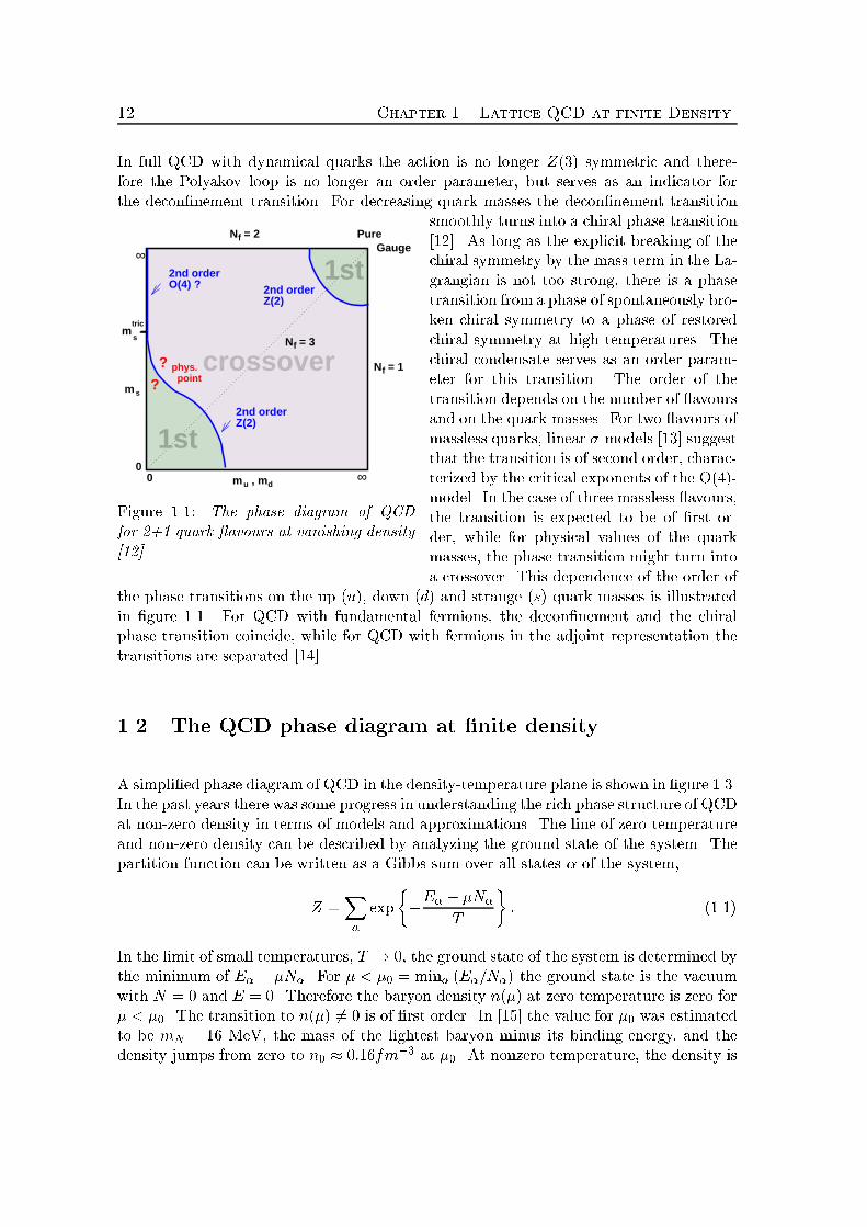
12 Chapter 1. Lattice QCD at finite DensityIn full QCD with dynamical quarks the action is no longer Z(3) symmetric and there-fore the Polyakov loop is no longer an order parameter, but serves as an indicator forthe decon�nement transition. For decreasing quark masses the decon�nement transition?

?phys.point

00

N = 2

N = 3

N = 1

f

f

f

m s

sm

Gauge

m , mu

1st

2nd orderO(4) ?

2nd orderZ(2)

2nd orderZ(2)

crossover

1st

d

tric

∞

∞Pure

Figure 1.1: The phase diagram of QCDfor 2+1 quark avours at vanishing density[12].

smoothly turns into a chiral phase transition[12]. As long as the explicit breaking of thechiral symmetry by the mass term in the La-grangian is not too strong, there is a phasetransition from a phase of spontaneously bro-ken chiral symmetry to a phase of restoredchiral symmetry at high temperatures. Thechiral condensate serves as an order param-eter for this transition. The order of thetransition depends on the number of avoursand on the quark masses. For two avours ofmassless quarks, linear �-models [13] suggestthat the transition is of second order, charac-terized by the critical exponents of the O(4)-model. In the case of three massless avours,the transition is expected to be of �rst or-der, while for physical values of the quarkmasses, the phase transition might turn intoa crossover. This dependence of the order ofthe phase transitions on the up (u), down (d) and strange (s) quark masses is illustratedin �gure 1.1. For QCD with fundamental fermions, the decon�nement and the chiralphase transition coincide, while for QCD with fermions in the adjoint representation thetransitions are separated [14].1.2 The QCD phase diagram at �nite densityA simpli�ed phase diagram of QCD in the density-temperature plane is shown in �gure 1.3.In the past years there was some progress in understanding the rich phase structure of QCDat non-zero density in terms of models and approximations. The line of zero temperatureand non-zero density can be described by analyzing the ground state of the system. Thepartition function can be written as a Gibbs sum over all states � of the system,Z =X� exp��E� � �N�T � : (1.1)In the limit of small temperatures, T ! 0, the ground state of the system is determined bythe minimum of E� � �N�. For � < �0 = min� (E�=N�) the ground state is the vacuumwith N = 0 and E = 0. Therefore the baryon density n(�) at zero temperature is zero for� < �0. The transition to n(�) 6= 0 is of �rst order. In [15] the value for �0 was estimatedto be mN � 16 MeV, the mass of the lightest baryon minus its binding energy, and thedensity jumps from zero to n0 � 0:16fm�3 at �0. At nonzero temperature, the density is

1.2. The QCD phase diagram at finite density 13not strictly zero. For small T and � one �nds a dilute gas of light mesons and nucleonswith n(T; �) � �T �2mNT� �3=2 e�mN =T : (1.2)Although the density is no longer zero below the transition for non-zero temperature,it is expected that the transition remains a �rst order phase transition for su�cientlysmall T . This nuclear gas-liquid transition line ends at a critical point at T � 10 MeV.

0

2

4

6

8

10

12

0 5 10 15 20

- (<E0>/<A0> - 2 MeV)----23

√10 <E0>/<A0>√√√√√√T

HeL

i (M

eV)

<E0>/<A0> (MeV)

197Au+197Au, 600 AMeV12C,18O +natAg,197Au, 30-84 AMeV22Ne+181Ta, 8 AMeV

Figure 1.2: Caloric curve of nuclei determined bythe dependence of the isotope temperature THeLion the excitation energy per nucleon [16].

Multi-fragmentation experiments atmoderate energies show signals forthis transition line [16]. Measure-ments of the yields of nuclear frag-ments show that the critical expo-nents are in agreement with those ofthe three-dimensional Ising model [17].In �gure 1.2 experimental signals forthe gas-liquid transition produced inAu + Au collisions at energies of 600MeV per nucleon are shown. Theplateau in this plot is related to al-most constant emission temperaturesover a broad range of incident ener-gies. This behaviour suggests a �rst-order phase transition with a substan-tial latent heat.For very high temperatures (T ��QCD), quarks and gluons form aplasma. The e�ective coupling con-stant g(T ) is logarithmically small andtherefore one can expect that the chiralcondensate is zero and therefore chiralsymmetry is restored at high tempera-tures due to asymptotic freedom. In the opposite region of the phase diagram, for smalltemperatures and large chemical potential, it is expected that chiral symmetry is alsorestored. For very large chemical potential (� � �QCD) the quarks occupy ever highermomentum states and due to asymptotic freedom, the interaction near the Fermi surfaceis weak. Non perturbative phenomena like chiral symmetry breaking should be absent atsu�ciently large �, therefore one can expect a phase transition where chiral symmetry isrestored. This transition is predicted to be of �rst order from the MIT bag model andrandom matrix model. The chiral condensate acts as a order parameter for this transition.At low temperatures, it is expected that additional interesting phases occur above thechiral-symmetry-restoring chemical potential [20]. It was suggested by Bailin and Love[21] that QCD at high density might behave analogous to a superconductor. Through theBCS mechanism [22], Cooper pairs of quarks condense in an attractive channel, breakingthe color gauge symmetry, and opening a gap at the Fermi surface. The coherent state,consisting of a quark pair condensate, has lower free energy than the perturbative vacuum,

14 Chapter 1. Lattice QCD at finite Density

Nucleon-Nucleoncollisions increasedensity and temperature

t ≅ 10-5

s

6 7 8

200

150

100

50

0

0 1 2 3 4 5

Neutron Stars

Density (relative to standard nuclear matter)

Cooling of the universe Quark-Gluon

plasmaT

empe

ratu

re [

MeV

]

Nuclearmatter

Hadron Gas

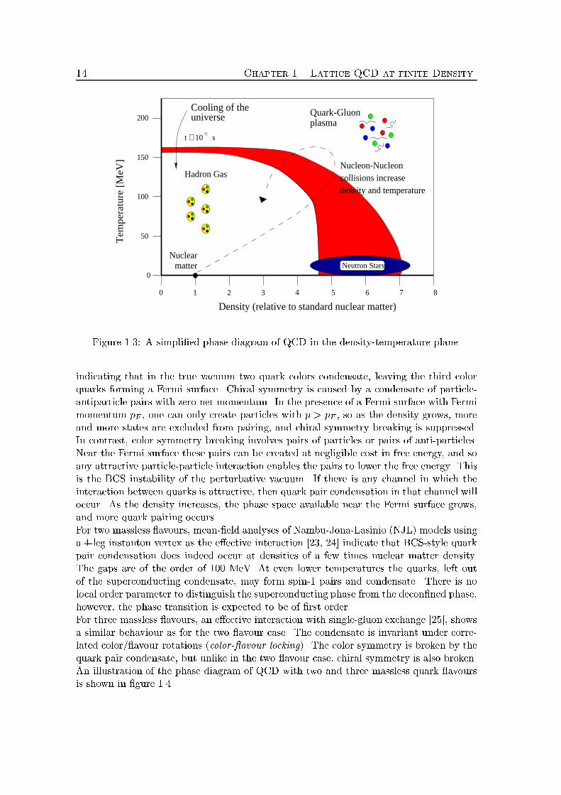
Figure 1.3: A simpli�ed phase diagram of QCD in the density-temperature plane.indicating that in the true vacuum two quark colors condensate, leaving the third colorquarks forming a Fermi surface. Chiral symmetry is caused by a condensate of particle-antiparticle pairs with zero net momentum. In the presence of a Fermi surface with Fermimomentum pF , one can only create particles with p > pF , so as the density grows, moreand more states are excluded from pairing, and chiral symmetry breaking is suppressed.In contrast, color symmetry breaking involves pairs of particles or pairs of anti-particles.Near the Fermi surface these pairs can be created at negligible cost in free energy, and soany attractive particle-particle interaction enables the pairs to lower the free energy. Thisis the BCS instability of the perturbative vacuum. If there is any channel in which theinteraction between quarks is attractive, then quark pair condensation in that channel willoccur. As the density increases, the phase space available near the Fermi surface grows,and more quark pairing occurs.For two massless avours, mean-�eld analyses of Nambu-Jona-Lasinio (NJL) models usinga 4-leg instanton vertex as the e�ective interaction [23, 24] indicate that BCS-style quarkpair condensation does indeed occur at densities of a few times nuclear matter density.The gaps are of the order of 100 MeV. At even lower temperatures the quarks, left outof the superconducting condensate, may form spin-1 pairs and condensate. There is nolocal order parameter to distinguish the superconducting phase from the decon�ned phase,however, the phase transition is expected to be of �rst order.For three massless avours, an e�ective interaction with single-gluon exchange [25], showsa similar behaviour as for the two avour case. The condensate is invariant under corre-lated color/ avour rotations (color- avour locking). The color symmetry is broken by thequark pair condensate, but unlike in the two avour case, chiral symmetry is also broken.An illustration of the phase diagram of QCD with two and three massless quark avoursis shown in �gure 1.4.

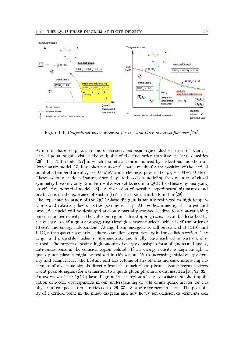
1.2. The QCD phase diagram at finite density 15170

chemicalpotential

Quark

superconducting

Temperature

SU(2)

A

A

Restoration of global symmetry

MeV

U(1)V

SU(2)

SU(2)

First order

confined

Second order

VSU(2) U(1)

U(1)V

SU(2)

ASU(2)

deconfined

ASU(2)

q qR R

color

hyper-nuclearmatter

L R

150MeV

qLqL

qLqR

chemicalpotential

Quark

superconducting

U(1)

U(1)SU(3) SU(3)

ASU(3)

ASU(3)

Temperature

Restoration of global symmetry

VU(1)

confined

SU(3)

BU(1)

SU(3)V

deconfined

Figure 1.4: Conjectured phase diagram for two and three massless avours [18].At intermediate temperatures and densities it has been argued that a critical or even tri-critical point might exist at the endpoint of the �rst order transition at large densities[26]. The NJL-model [27] in which the interaction is induced by instantons and the ran-dom matrix model [15] have shown almost the same results for the position of the criticalpoint of a temperature of Ttc � 100 MeV and a chemical potential of �tc � 600�700 MeV.These are only crude estimates, since they are based on modeling the dynamics of chiralsymmetry breaking only. Similar results were obtained in a QCD-like theory by analyzingan e�ective potential model [28]. A discussion of possible experimental signatures andpredictions on the existence of such a (tri)critical point can be found in [29].The experimental study of the QCD phase diagram is mainly restricted to high temper-atures and relatively low densities (see �gure 1.5). At low beam energy the target andprojectile nuclei will be destroyed and only partially stopped leading to a non-vanishingbaryon number density in the collision region. This stopping scenario can be described bythe energy loss of a quark propagating through a heavy nucleon, which is of the order of10 GeV and energy independent. At high beam energies, as will be realized at RHIC andLHC, a transparent scenario leads to a smaller baryon density in the collision region. Thetarget and projectile nucleons interpenetrate and �nally leave each other partly undis-turbed. The targets deposit a high amount of energy density in form of gluons and quark,anti-quark pairs in the collision region behind. If the energy density is high enough, aquark gluon plasma might be realized in this region. With increasing initial energy den-sity and temperature, the lifetime and the volume of the plasma increase, improving thechances of observing signals directly from the quark gluon plasma. Some recent reviewsabout possible signals for a transition to a quark gluon plasma are discussed in [30, 31, 32].An overview of the QCD phase diagram in the region of large densities and the impli�-cation of recent developments in our understanding of cold dense quark matter for thephysics of compact stars is reviewed in [26, 33, 18] and references in there. The possibil-ity of a critical point in the phase diagram and how heavy ion collision experiments can

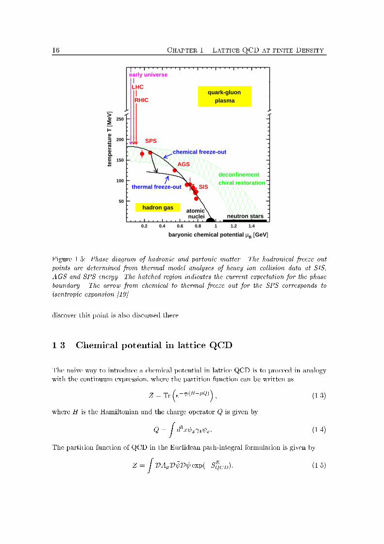
16 Chapter 1. Lattice QCD at finite Density

0.2 0.4 0.6 0.8 1 1.2 1.4

50

100

150

200

250

early universe

LHC

RHIC

baryonic chemical potential µB [GeV]

tem

per

atu

re T

[MeV

]

SPS

AGS

SIS

atomicnuclei neutron stars

chemical freeze-out

thermal freeze-out

hadron gas

quark-gluonplasma

deconfinementchiral restoration

Figure 1.5: Phase diagram of hadronic and partonic matter. The hadronical freeze outpoints are determined from thermal model analyses of heavy ion collision data at SIS,AGS and SPS energy. The hatched region indicates the current expectation for the phaseboundary. The arrow from chemical to thermal freeze out for the SPS corresponds toisentropic expansion [19].discover this point is also discussed there.1.3 Chemical potential in lattice QCDThe naive way to introduce a chemical potential in lattice QCD is to proceed in analogywith the continuum expression, where the partition function can be written asZ = Tr�e� 1T (H��Q)� ; (1.3)where H is the Hamiltonian and the charge operator Q is given byQ = Z d3x � x 4 x: (1.4)The partition function of QCD in the Euclidean path-integral formulation is given byZ = Z DA�D � D exp(�SEQCD): (1.5)

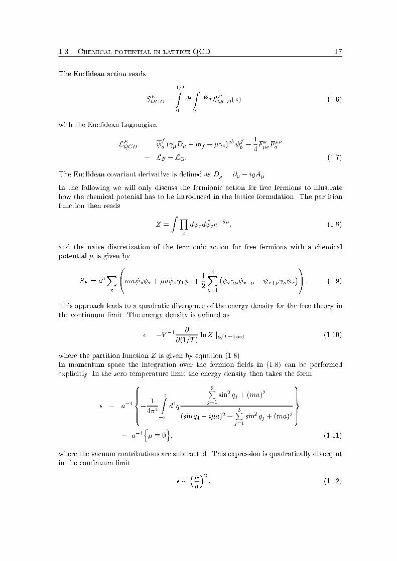
1.3. Chemical potential in lattice QCD 17The Euclidean action readsSEQCD = 1=TZ0 dtZV d3xLEQCD(x) (1.6)with the Euclidean LagrangianLEQCD = fa ( �D� +mf + � 4)ab fb + 14F a��F ��a= LF + LG: (1.7)The Euclidean covariant derivative is de�ned as D� = @� � igA�.In the following we will only discuss the fermionic action for free fermions to illustratehow the chemical potenial has to be introduced in the lattice formulation. The partitionfunction then reads Z = Z Yx d xd � xe�SF ; (1.8)and the naive discretization of the fermionic action for free fermions with a chemicalpotential � is given bySF = a3Xx 0@ma � x x + �a � x 4 x + 12 4X�=1 � � x � x+� � � x+� � x�1A : (1.9)This approach leads to a quadratic divergence of the energy density for the free theory inthe continuum limit. The energy density is de�ned as� = �V �1 @@(1=T ) lnZ j�=T=�xed (1.10)where the partition function Z is given by equation (1.8).In momentum space the integration over the fermion �elds in (1.8) can be performedexplicitly. In the zero temperature limit the energy density then takes the form� = a�48>>><>>>:� 14�4 �Z�� d4q 3Pj=1 sin2 qj + (ma)2(sin q4 � i�a)2 + 3Pj=1 sin2 qj + (ma)29>>>=>>>;� a�4n� � 0o; (1.11)where the vacuum contributions are subtracted. This expression is quadratically divergentin the continuum limit � � ��a�2 : (1.12)

18 Chapter 1. Lattice QCD at finite DensityA similar divergence occurs for the particle number density. This problem is not connectedto the occurrence of fermion doublers due to additional zero modes in the free propaga-tor. It also appears in the Wilson formulation for the fermionic action where the 16-folddegeneracy of eq. (1.11) is removed. The divergence is not a lattice artifact, but is alsopresent in the continuum theory itself, where one uses some prescription, like the contourmethod, to get rid of it. A class of actions that get rid of this divergence in lattice QCDwere proposed by Gavai [34]. The most common prescription was introduced by Karschand Hasenfratz [35]:SF = a3Xx �ma � x x + 12 3X�=1 � � x � x+� � � x+� � x�+ 12 �e�a � x 4 x+4 � e��a � x+4 4 x�� : (1.13)This expression now leads to the following expression for the energy density in momentumspace in the zero temperature limit� = a�48>>><>>>:� 14�4 �Z�� d4q 3Pj=1 sin2 qj + (ma)2sin2(q4 � i�a) + 3Pj=1 sin2 qj + (ma)29>>>=>>>;� a�4n� � 0o: (1.14)(1.15)After performing the q4 integration one gets� = a�4 12�3 Z ��� d3q�(e�a � b�pb2 + 1) bb2 + 1 (1.16)with b2 = 3Xj=1 sin2 qj + (ma)2: (1.17)In the continuum limit, a! 0, this expression leads to the correct result for the momentumcut-o� � �(��p~q2 +m2) in every corner of the Brillouin zone and reproduces 16 timesthe usual energy density of free fermions at zero temperature,� = 16 �0 (1.18)�0 = �44�2 : (1.19)The particle number density nq can be derived in the same way and one reproduces 16times the continuum value, nq = 16 n0 (1.20)n0 = �33�2 : (1.21)

1.4. Problems in simulating QCD at finite density 19For the Wilson formulation of the fermionic action, the chemical potential can be includedanalogous to (1.13),SF (�a) = Xx ( � x x � � 3Xj=1[ � x(1� j)Ux;j x+j + � x+j(1 + j)U yx;j x]��[e�a � x(1� 4)Ux;4 x+4 + e��a � x+4(1 + 4)U yx;4 x]): (1.22)The degeneracy is removed for Wilson fermions and the factor 16 in (1.18) and (1.20)disappears.Together with the gluonic action the grand canonical partition function readsZgc(T; V; �) = Z D � D DUe�SG(U)�SF ( � ; ;U): (1.23)The standard Wilson discretization of the gluonic action can be written asSG = � Xn;�<��4 �1� 12NcTrfU��(n) + U y��(n)g� (1.24)with the usual de�nition � = 2Ncg2 and the Plaquette terms de�ned byU�;� = U�(n)U�(n+ a�)U y�(n+ a�)U y� (n): (1.25)For the staggered formulation of the fermionic action, the chemical potential can be in-troduced in analogy to (1.13) and (1.22).Considering the way of introducing a chemical potential discussed above at �nite temper-ature, forward quark propagation, in terms of quark loops wrapping around the lattice inthe imaginary time direction, is enhanced by a factor e�a while forward propagation ofanti-quarks is damped by a factor e��a. For ordinary closed paths in spatial direction the� dependence cancels, as these loops describe virtual pair creation and annihilation andthe chemical potential for quarks and anti-quarks is of opposite sign. We will see later thatthis way of including the chemical potential in lattice QCD will lead to a quite naturalextension of the calculation scheme for thermodynamic quantities in terms of a hoppingparameter expansion for the Wilson formulation of the fermion action at non-zero density.1.4 Problems in simulating QCD at �nite densityThe usual approach to include dynamical fermions in lattice QCD is to integrate themout. Due to the Grassmann properties of fermion �elds this leads to a determinant of thefermion matrix, Z = Z DUD � D e�SG(U)� � M(U) = Z DUdetM(U)e�SG(U) (1.26)

20 Chapter 1. Lattice QCD at finite Densityand an e�ective action depending only on the gauge �elds. Monte Carlo simulations requirea positive integrand in the partition function, because of the probabilistic interpretationof the path integral. One way to guarantee this is if M is similar to its adjoint, so theeigenvalues are real or in complex-conjugate pairs,M y = PMP�1 for some P: (1.27)For the Wilson formulation of the fermion matrix,Mx;y = �x;y � � 3Xj=1[(r � j)Ux;j�x;y�j + (r + j)U yx;j�x;y+j ]��[e�a(r � 4)Ux;4�x;y�4 + e��a(r + 4)U yx;4�x;y+4]) (1.28)M yx;y = �x;y � � 3Xj=1[(r + j)U yx;j�x;y+j + (r � j)Ux;j�x;y�j ]��[e�a(r + 4)U yx;4�x;y+4 + e��a(r � 4)Ux;4�x;y�4]); (1.29)the relation (1.27) is ful�lled for P = 5 and zero chemical potential or purely imaginarychemical potential, M y = 5M 5 ; for � = i� with � 2 R: (1.30)Introducing a real chemical potential, (1.30) is no longer valid and the fermion determi-nant is then complex. This is the sign problem which is really a phase problem for QCD.For QCD with only two colors, the relation (1.27) is true for P = �2 and any chemicalpotential and the fermion determinant is real and positive. For any number of colors andfermions in the adjoint representation the fermion determinant is real. All above casescan be classi�ed by a Dyson index, i.e. the number of independent degrees of freedom permatrix element [36].1.5 The naive quenched limitBecause of the complex fermion determinant, Monte Carlo simulations in QCD with non-zero chemical potential were mainly restricted to the quenched approximation. Problemsin this approach were �rst reported in [37]. In contrast to the expected behaviour, thatthe onset transition, i.e. the transition from zero to non-zero density, at zero tempera-ture occurs at a critical chemical potential related to the lightest baryon in the theory,�0 = mN=3, where mN is the nucleon mass, in quenched simulations the onset was foundat an unphysical value of half the pion mass, i.e. �0 = m�=2. In the chiral limit thiswould extrapolate to zero and chiral symmetry would be restored for all non-zero �. Thisbehaviour was also veri�ed in simulations on large lattices [38, 39]. A review of the prob-lems in simulating QCD at non-zero density can be found in [40].

1.6. Alternative approaches to finite density 21The failure of the quenched approximation at non-zero chemical potential was �rst under-stood analytically in terms of chiral random matrix theory [41]. The quenched limit canbe interpreted as the limit Nf ! 0 of a partition function with the absolute value of thefermion determinant, jdet(D(�) +m)jNf ; (1.31)rather than (det(D(�) +m))Nf : (1.32)The absolute value of the fermion determinant can be written asdet(D(�) +m) det(Dy(�) +m): (1.33)Writing the fermion determinant as a Grassmann integral, one observes that the quenchedpartition function can be interpreted as a partition function of quarks and conjugate anti-quarks. Therefore in addition to the usual Goldstone-modes, the quenched theory containsGoldstone modes consisting of a quark and a conjugate anti-quark [41, 42]. Such modeswith the same mass as the usual Goldstone modes, i.e. the pions, have a non-zero baryonnumber. The critical chemical potential given by the mass of the lightest particle with non-zero baryon number is thus m�=2. This explains why the naive quenched limit describesthe wrong physics. In the following sections we will derive the correct quenched or in otherwords static limit in two alternative approaches.1.6 Alternative approaches to �nite densityThe baryon number conservation law tells us that the di�erence between the number ofparticles and the number of anti-particles, i.e. the baryon number B = N � �N , is con-served. This means that a particle can be created or annihilated only in conjunction withan anti-particle. At low temperatures the thermal energy is not su�cient to create pairs,therefore the number of particles is e�ectively conserved. At high temperatures the pos-sibility of pair creation has to be taken into account. There will be an average numberof particles and anti-particles present in equilibrium and there will also be uctuationsabout the average value, while the di�erence between particle and anti-particle numbersremains strictly constant and is determined by the initial conditions.In relativistic statistical mechanics, we have the choice between the grand canonical andthe canonical treatments of conservation laws. While in the canonical approach the baryonnumber is conserved exactly, it is the average value of the baryon number which is con-served in the grand canonical description. If the baryon number and the volume takeon very large values with B=V ! const, the grand canonical approach is adequate, forexample in cosmology and astrophysics. In many other realistic physical situations theapplication of the grand canonical ensemble with respect to the conservation laws can bequestionable, especially when dealing with a small amount of matter enclosed in a tinyvolume with a small absolute value of the quantum numbers. This situation is found in the

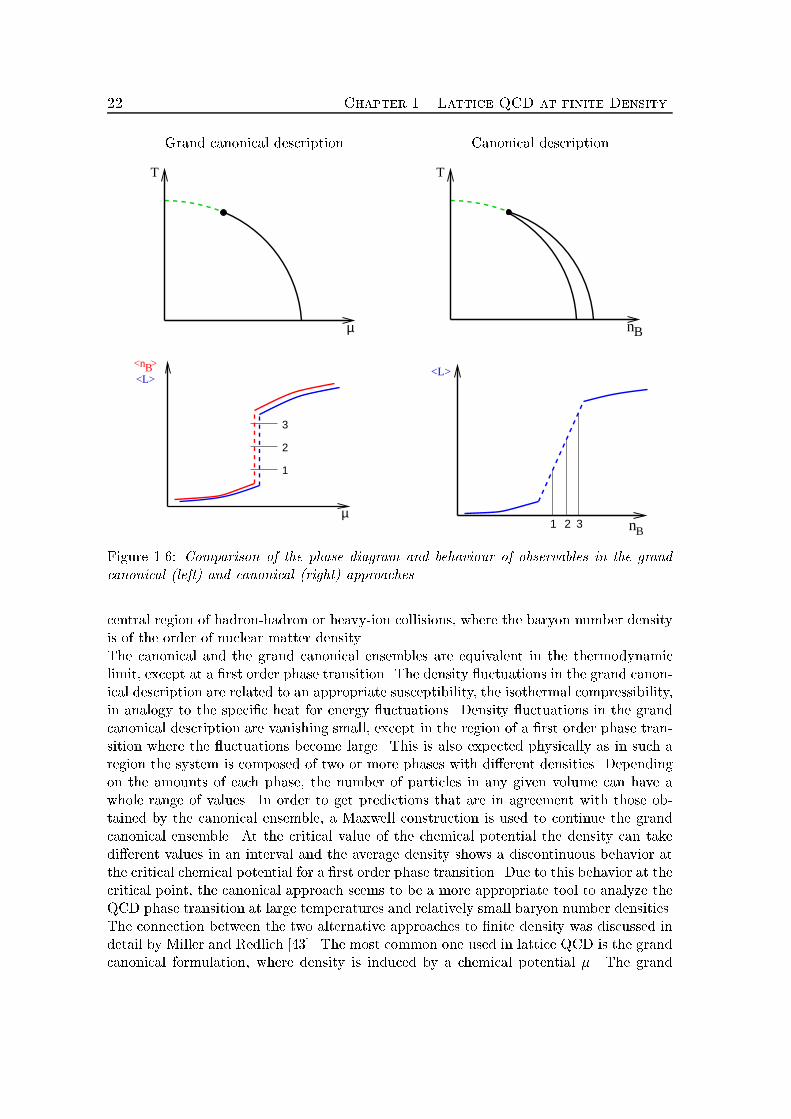
22 Chapter 1. Lattice QCD at finite DensityGrand canonical descriptionT

µ

<L>

<n >B

1

2

3

µ

Canonical descriptionT

nB

<L>

nB1 2 3Figure 1.6: Comparison of the phase diagram and behaviour of observables in the grandcanonical (left) and canonical (right) approaches.central region of hadron-hadron or heavy-ion collisions, where the baryon number densityis of the order of nuclear matter density.The canonical and the grand canonical ensembles are equivalent in the thermodynamiclimit, except at a �rst order phase transition. The density uctuations in the grand canon-ical description are related to an appropriate susceptibility, the isothermal compressibility,in analogy to the speci�c heat for energy uctuations. Density uctuations in the grandcanonical description are vanishing small, except in the region of a �rst order phase tran-sition where the uctuations become large. This is also expected physically as in such aregion the system is composed of two or more phases with di�erent densities. Dependingon the amounts of each phase, the number of particles in any given volume can have awhole range of values. In order to get predictions that are in agreement with those ob-tained by the canonical ensemble, a Maxwell construction is used to continue the grandcanonical ensemble. At the critical value of the chemical potential the density can takedi�erent values in an interval and the average density shows a discontinuous behavior atthe critical chemical potential for a �rst order phase transition. Due to this behavior at thecritical point, the canonical approach seems to be a more appropriate tool to analyze theQCD phase transition at large temperatures and relatively small baryon number densities.The connection between the two alternative approaches to �nite density was discussed indetail by Miller and Redlich [43]. The most common one used in lattice QCD is the grandcanonical formulation, where density is induced by a chemical potential �. The grand

1.7. The propagator matrix 23canonical partition function Zgc(T; V; �) depends on the temperature T , the Volume Vand �. In this formulation, the physical baryon density is an observable, depending onthe chemical potential �, and is conserved in terms of the average value of the baryonnumber. Monte Carlo simulations in this formulation su�er from the fact that the fermiondeterminant gets complex for non-zero �. This sign problem was discussed in detail byBarbour et al. [44]. In the static limit, mq; �!1, keeping e�=mq �xed, as proposed byBender et al. [45] ,this can be handled for moderate lattice sizes. Simulations in this limitfor staggered fermions were performed by Blum et al. [46] and for Wilson fermions in thiswork (see Chapter 4).Instead of working with a chemical potential, one can directly �x the quark number den-sity B, i.e. the baryon number density B=3, by introducing a complex chemical potentialin the grand canonical partition function and performing a Fourier transformation [43].This transformation projects onto canonical partition functions at �xed quark number B,Zc(B;T; V ) = 12� Z 2�0 d�e�iB�Zgc(i�; T; V ): (1.34)Instead of a complex fermion determinant, the problem of this approach is the heavilyoscillating integrand in (1.34). We will see later that this can be handled in the quenchedlimit, i.e. for in�nite quark mass, as the Fourier integral can be performed explicitlyafter an expansion of the action in terms of the hopping parameter. What remains is asign problem which can be handled for lattice sizes up to 163 � 4, small densities andtemperatures down to 0:8Tc.A qualitative di�erence of these approaches is described in �gure 1.6. In the phase diagramin the T -� plane, the phase transition occurs at a speci�c value of the chemical potential,�c. For a �rst order transition, observables like the Polyakov loop L or the baryon numberdensity nB show a discontinuous behaviour at �c. In the canonical approach, nB is nolonger an observable, but a parameter of the theory. It can be written in units of thetemperature T cubed as nBT 3 = B3 �N�N��3 ; (1.35)where B is the number of quarks, i.e. B=3 is the baryon number and N� and N� arethe lattice extensions in temporal and spatial direction. By varying the baryon numberdensity one can traverse the region of coexisting phases (the discontinuity in the grandcanonical approach at �c) continously. Therefore observables are continuous in the densityeven for a �rst order phase transition and the transition occurs in a density interval. Inthe phase diagram in the T -nB plane an additional region of coexisting phases occurs.1.7 The propagator matrixThe two alternative approaches to lattice QCD at non-vanishing density, discussed in theprevious section, can be compared in a nice way in the following example. For the stag-gered formulation of the fermionic action, the connection between the canonical and grand

24 Chapter 1. Lattice QCD at finite Densitycanonical partition functions can be analyzed in terms of a propagator matrix descriptionproposed by Gibbs [47]. The grand canonical partition function can be expanded in termsof canonical partition functions, each for a �xed number of fermions on the lattice. Thisexpansion can be obtained as a characteristic polynomial of a propagator matrix P . Eachof the canonical partition functions can be expressed in terms of traces of powers of P .In the following we derive the propagator matrix formalism for the case of staggeredfermions. The fermion matrix M can be rede�ned asM = iM = G+ V e� + V ye�� + im; (1.36)where the matrix G contains the contribution to M from the space-like links and is her-mitian, V is the contribution from the forward time-links and m is the bare quark mass.The propagator matrix P can now be de�ned asP = � �G� im 1�1 0 �V (1.37)and the inverse of P is given byP�1 = V y� 0 �11 �G� im � : (1.38)The matrix P is related to the determinant of the fermion matrix bydet(M) = det(M) = e3V �det(P � e��) (1.39)As the matrix (P � e��) is diagonal in the fugacity e��, it can be expanded as a charac-teristic polynomial in the fugacity,det(P � e��) = e�6V �det(e� � P�1) = e�6V � 6VXn=0 !nen�; (1.40)where the coe�cients !n are given by the recurrence relationTrP n + n�1Xi=1 !iTrP n�i + n!n = 0 (1.41)with !0 = 1 and !1 = �TrP . Since the propagator matrix causes a step forward in time,TrP n is non-zero only when n is a multiple of N� , the temporal extend of the lattice, andwe can de�ne !n = !nN� (1.42)By considering the hermitian conjugate of (1.39) one can show the following relation:!n = !�6V�n: (1.43)The formal expansion of the grand canonical partition function in terms of the canonicalones is now = 3VXn=0!ne�(3V �n)N�� + !�ne(3V �n)N��Zgc(�; T; V ) = Z DUe�SG (1.44)

1.8. The canonical partition function 25Using the Fourier transformation (1.34) one can see that the canonical partition functionfor B=(3V � n) fermions on the lattice is given byZc(B;T; V ) = 12� Z 2�0 d�e�iB�Zgc(i�; T; V )= Z DU!Be�SG (1.45)Due to the Z(3) symmetry, the canonical partition functions are non-zero only when B is amultiple of 3. Furthermore, they are real when integrating over all gauge �elds. Equation(1.44) together with the relation (1.43) shows that the fermion determinant is real for� = 0 and for imaginary chemical potential. While for real and non-zero � the fermiondeterminant gets complex.1.8 The canonical partition functionThe connection between the grand canonical and the canonical formulation of QCD wasdiscussed in section 1.6. The main problem arises from the fact that the integrand inthe Fourier transformation, which eliminates the dependence on the chemical potentialin favour of a �xed quark number, is highly oscillating. We will now derive an explicitexpression for the canonical partition functions for Wilson fermions in terms of a hoppingparameter expansion as discussed in [1]. The Fourier integral can then be performedexplicitly. Later on we will concentrate on the leading order in the hopping parameter �,which is all one needs to perform the quenched limit (�! 0).Rewriting the fermionic action (1.22) by transforming the fermion �elds 0(~x;x4) = e�ax4 (~x;x4) ; � 0(~x;x4) = e��ax4 � (~x;x4) (1.46)shifts the dependence on the chemical potential into only the last time slice. The �-independent part of the action may be written as~SF = SF (0) � SN�F (0); (1.47)where SN�F is the only �-dependent part of the fermionic action. Using the de�nition ofthe temperature 1=T = aN� this part can be expressed in terms of �=T = �aN� ,SN�F (�=T ) = �X~x [e�=T � (~x;N� )(1� 4)Ux;4 (~x;1) + e��=T � (~x;1)(1 + 4)U yx;4 (~x;N� )]: (1.48)The chemical potential can now be completely removed from the action by including the�-dependence in the generalized boundary conditions (~x;N�+1) = �e�=T (~x;1) ; � (~x;N�+1) = �e��=T � (~x;1): (1.49)The grand canonical partition function at a chemical potential �=T = �aN� in a volumeV = (N�a)3 at temperature T = 1=N�a now readsZgc(�=T ; T; V ) = Z Yx;� dUx;�Yx d � xd xe�SN�F (�=T )e�SG� ~SF ; (1.50)

26 Chapter 1. Lattice QCD at finite Densitywhere SG denotes the gluonic action, which is �-independent. For the gluonic sector weuse the standard Wilson formulation (1.24). The Fourier transformation only acts on the�-dependent part e�SN�F , which only involves links pointing in the 4th direction on thelast time slice of the lattice. Using the Grassmann properties of the fermionic �elds thiscontribution can be written ase�SN�F (i�) = Y(~x;a;b;�;�;f) (1� �ei� � a;�;f(~x;N� )Ua;�;b;�~x b;�;f(~x;1) )� (1.51)(1� �e�i� � a;�;f(~x;1) Uya;�;b;�~x b;�;f(~x;N� )); (1.52)where the product runs over all possible combinations of indices with ~x taking values onthe three dimensional (spatial) lattice of size N3� , � = 1; :::; 4 and a = 1; 2; 3 denotingthe spinor and color indices and f = 1; :::; nf for di�erent fermion avours. We haveignored the possibility of having di�erent quark masses, i.e. di�erent hopping parameters� for various avours. In the following we will combine the spinor and color indices byA = (�; a). In (1.52) we have used the notationU~x = ��U(~x;N� );4 ; Uy~x = �+U y(~x;N� );4 ; with �� = (1� 4) (1.53)Each propagator term in (1.52) comes with a hopping parameter � and with a complexfugacity z = exp(i�) for the forward propagator, respectively z� for the backward propaga-tor. Expanding this product in terms of the fugacity results in terms that are proportionalto zn��n and �n+�n, where n denotes the number of forward and �n the number of backwardpropagating terms. The Fourier transformationZc(B;T; V ) = 12� Z 2�0 d� e�iB�Zgc(i�; T; V ): (1.54)will receive a non-zero contribution only from terms with n � �n = B, i.e. terms thatare proportional to zB . In the following we will only concentrate on the leading order inthe hopping parameter �. As each non-vanishing term in the Fourier transformation isproportional to �n+�n, the leading order in a hopping parameter expansion arises from the�n � 0 sector and can be summarized aszBfB � (�z�)B XX;C;D;F BYi=1 � Ci;fi(~xi;N� )UCi;Di~xi Di;fi(~xi;1); (1.55)where X, C, D, F are B-dimensional vectors, i.e. X = (~x1; :::; ~xB), F = (~f1; :::; ~fB) and soon. All elements of the set f(Ci; fi; ~xi)gBi=1 as well as f(Di; fi; ~xi)gBi=1 have to be di�erentto give a non-vanishing contribution to the sum in (1.55). The Fourier integral (1.54) cannow be performed explicitly and one obtains the canonical partition functionZ(B;T; V ) = Z Yx;� DUx;�Yx d xd xfBe�SG� ~SF (1.56)at �xed baryon (or quark) number, where the �xed quark number B is encoded in thefunction fB as a sum over products of quark propagators between the time slice x4 = 1 and

1.8. The canonical partition function 27x4 = N� . In the following B denotes the quark number. Therefore the physical baryonnumber is given by B=3.In a hopping parameter expansion (heavy quark mass limit) for the entire fermion determi-nant, the function fB is all we need to generate the leading contribution, which �nally willbe O(�BN� ). To this order only B quark loops that wind around the temporal direction ofthe lattice contribute to the determinant. In the next order in � additional factors from anexpansion of exp(� ~SF ) have to be included. In higher orders additional factors of (1.52)which have to contain an equal number of additional backward and forward propagatingterms lead to contributions of anti-quarks.As we want to perform the quenched limit in this approach, we will now have a moredetailed look at the leading contribution arising from fB. To simplify this, we performa gauge transformation such that all the links pointing in the time direction on the lasttime slice are equal to unity. As these are the only gauge �elds that contributed, fB nowonly depends on the fermionic �elds on the last time slice,fB = (�2�)B XX;A;F BYi=1 � Ai;fi(~xi;N� ) Ai;fi(~xi;1): (1.57)As only two components of �� are non-zero, the spinor indices �i which are part of Ai nowonly take on the values �i = 1; 2. This also gives rise to the factor 2 in front of �. Whenevaluating the Grassmann integrals each of the � terms can be contracted with all those terms which carry the same avour index. Each pair gives rise to a matrix element ofthe inverse of ~Q, the fermion matrix corresponding to ~SF . The di�erent pairings give riseto the Matthews-Salam determinant. We will get the product of nf determinants, each ofdimension dl such that Pnfl=1 = B,fB = (2�)B XX;A;F nfYl=1 detMl[x;A] (1.58)where the matrixMl gives the contributions for the l� th avour and the matrix elementsare the corresponding quark propagators,Mi;jl = ~Q�1((~xj ;1);Aj);((~xi;N� );Ai): (1.59)Each matrix element of Ml is O(�(N��1+j~xi�~xj j)). In the heavy quark mass limit (� !0), only matrix elements with j~xi � ~xjj = 0 will contribute. In this case the elementsQ�1((~xi;1);Aj);((~xi;N� );Ai) are just products of terms ��U(~xi;k);4 with k = 1; :::; N� � 1. As ��is a diagonal matrix in spinor space the indices �i and �j have to be identical. The spinorpart thus gives rise to an overall factor 2N��1 for each i, i.e. we obtain B such factors. Themultiplication of the SU(3) matrices yields an element of the ordinary, complex valuedPolyakov loop (U � 1 on the last time slice) which we denote by Lai;aj~xi . Finally, the sumover di�erent color indices appearing in (1.58) leads to contributions involving only tracesover powers of the Polyakov loop,L~x = N�Yx4=1U(~x;x4): (1.60)

28 Chapter 1. Lattice QCD at finite DensityAs the (color, spinor) label Ai can take on six di�erent values, the determinant is non-zeroonly if at most six quarks of a given avour occupy a given site ~xi. In the quenched limitthe partition function now readsZ(B;T; V ) = Z Yn;� DU�(n)fBe�SG : (1.61)A more detailed description of the canonical partition function and a general derivation ofthe functions fB can be found in [1]. A more straightforward derivation of the canonicalpartition functions in the quenched limit will be discussed in the following section inconnection to the grand canonical approach.1.9 The grand canonical partition functionWe will now have a look at the grand canonical partition function. We will derive thequenched, i.e. static limit, in this approach analogous to the derivation in [46] and showthat the canonical partition functions of the previous section can be derived in a quitenatural way analogous to the propagator matrix formalism discussed in section 1.7.The fermion matrix for Wilson fermions at non-zero chemical potential is given byMx;y = �x;y � � 3Xj=1[(1� j)Ux;j�x;y�j + (1 + j)U yx;j�x�j;y]��[e�a(1� 4)Ux;4�x;y�4 + e��a(1 + 4)U yx;4�x�4;y])= 11� �G� �(1 � 4)e�V � �(1 + 4)e��V y (1.62)In the quenched limit one has to perform the limit �! 0 and �!1, keeping the ratio �e��xed [45]. As we have already seen in the canonical approach, only forward propagatingterms in temporal direction contribute in this limit,Mx;y � 11� �(1 � 4)e�V: (1.63)Each spatial point is decoupled from all others and the fermion matrix can be written asM = 0BBBBB@ 1 �C�1=N�V0 0 : : : 00 1 �C�1=N�V1 : : :0 0 1... ... . . . �C�1=N�VN��1C�1=N�VN� 11CCCCCA (1.64)with C = (2�e�a)�N� : (1.65)The matrices Vi are diagonal in the spatial indices,Vi = Diag�12(1� 4)U4(~x; x4 = i); ~x� : (1.66)

1.9. The grand canonical partition function 29The fermion matrix can now be diagonalized and the fermion determinant is expressed asa product of determinants of local Polyakov loops P~x =Qx4 U4(~x; x4),det(M) = C�12V Y~x det(��P~x + C) (1.67)= C�6V Y~x (det(P~x + C))2 (1.68)= C�6V Y~x (C3 + C2TrP~x + CTrP y~x + 1)2 (1.69)= Y~x (C�3 + C�2TrP y~x + C�1TrP~x + 1)2 (1.70)= Y~x (det(P y~x + C�1))2: (1.71)This expression is comparable to the one obtained for the staggered formulation in [46]except for the square of the local determinants. The square enters here due to the spinorstructure of the Wilson formulation.The physical quark density is given by the derivative of the logarithm of the partitionfunction with respect to the chemical potential byhni = 1aN�V @ln(Z)@� (1.72)= 2V *X~x C2TrP~x + 2CTrP y~x + 3C3 + C2TrP~x + CTrP y~x + 1+ : (1.73)One can now de�ne a propagator matrix P byP = 0BBBBB@ P0 0 0 0 00 P0 0 0 00 0 . . . 0 00 0 0 P~x 00 0 0 0 P~x1CCCCCA (1.74)and the fermion determinant can be expanded as a characteristic polynomial in the coef-�cient C, det(M) = C�6V det(P + C) (1.75)= det(P y + C�1) (1.76)= 6VXn=0C�n!n (1.77)= C�6V 6VXn=0Cn!�n ; (1.78)

30 Chapter 1. Lattice QCD at finite Densitywhere the !n are given by the recurrence relation(�1)nTrP n + n�1Xi=1(�1)n�i!iTrP n�i + n!n = 0 (1.79)with !0 = 1 and !1 = TrP and the symmetry !n = !�6V�n. The coe�cients !n can nowbe interpreted as the canonical partition functions at a �xed quark number B = n andone can show that they are identical to the partition functions derived in the last section.The �rst coe�cients are given by!0 = 1 (1.80)!1 = TrP = 2X~x TrP~x (1.81)!2 = 12 ��TrP 2 + (TrP )2� = �X~x TrP 2~x + 2 X~x TrP~x!2 (1.82)!3 = 13 �TrP 3 � 32TrP 2TrP + 12 (TrP )3� (1.83)= 13 0@2X~x TrP 3~x � 6X~x TrP 2~xX~x TrP~x + 4 X~x TrP~x!31A (1.84)The canonical partition functions now readZ(B;T; V ) = Z Yn;� DU�(n)!Be�SG (1.85)and are equivalent to the ones derived in the previous section and discussed in [6]. Theequivalence, !B = fB, can be seen quite easily by using some calulation rules for the tracesof SU(3)-matrices. Because of the Z(3)-symmetry of the action SG, the partition functionsare non-zero only if B is a multiple of 3.The recurrence relation (1.79) can be rewritten to!n = � n�1Xi=0 2n(�1)n�i!iX~x Tr P n�i~x ; with (1.86)!0 = 1Therefore the functions fB = !B can be evaluated for all B and have a more compactform than the expressions derived in [1].

Chapter 2Observables at �nite temperatureand density2.1 Thermodynamic observablesThe calculation of the equation of state of QCD is one of the central goals of latticesimulations at �nite temperature. The behaviour of thermodynamic observables like thepressure p, the energy density � and the entropy density s are of great interest for theunderstanding of the QCD phase transition and the high temperature phase as it mighthave existed in the early universe and be produced in heavy ion collisions. The intuitivepicture of the high temperature phase as a gas of weakly interacting quarks and gluonsis based on leading order perturbation theory. Perturbative QCD fails to describe theequation of state even at rather high temperatures because of infrared problems of thetheory. It seems that non-perturbative e�ects still dominate the equation of state in thetemperature regime attainable in heavy ion collisions.The high temperature behaviour of QCD is close to that of an ideal gas. Bulk thermo-dynamic quantities are therefore dominated by contributions from large momenta. Theseare most strongly in uenced by �nite cut-o� e�ects. Calculations of the energy density,entropy density and pressure in SU(3) gauge theory with the standard Wilson actionwere performed by Boyd et al. [48]. They show a strong cut-o� dependence which is ofO((aT )2) and the deviations from the ideal gas limit are about 15% even at temperatureof about 5Tc. In [49] and [50] it was shown that these cut-o� e�ects can be reduced to afew percent by using tree level or tadpole improved actions even on lattices with temporalextent as small as N� = 4.The thermodynamic quantities in lattice QCD can be calculated using basic thermody-namic relations in the continuum. All quantities can be derived from the partition functionZ(T; V; �). Its logarithm de�nes the free energy density,f = �TV lnZ(T; V; �): (2.1)31

32 Chapter 2. Observables at finite temperature and densityThe energy density and pressure are derivatives of lnZ with respect to T and V ,� = T 2V @ lnZ(T; V; �)@T ����=T �xed (2.2)p = T @ lnZ(T; V; �)@V ����=T �xed (2.3)As the logarithm of the partition function is not directly accessible within the Monte Carloapproach, the free energy density is calculated from an integration of its derivative withrespect to �, �@ lnZ@� = hSGi = 6N3�N�PT ; (2.4)where SG is the gluonic part of action and PT denotes the plaquette expectation value attemperature T calculated on a lattice of sizeN3�N� . If P0 denotes the plaquette expectationvalue, evaluated on a lattice of sizeN4� , the di�erence of the free energy density at couplings� and �0 is obtained as fT 4 j��0 = �6N4� Z ��0 d�0[P0 � PT ]: (2.5)This relation can also be used to calculate the free energy density at non-zero densities,while the following relations only hold for � = 0. For large, homogeneous systems thefollowing relation, lnZ = V @ lnZ@V (2.6)can be used to show that the pressure can directly be obtained from the free energy density,p(�) = �[f(�)� f(�1)]; (2.7)with the assumption that �1 has to be small enough, so that p(�1) is approximately zero.Using the relation (2.7) one can express the entropy density s and the interaction measure� in terms of derivatives of the pressure with respect to the temperature,s = �+ pT = @p@T (2.8)� = �� 3pT 4 = T @@T �p=T 4� (2.9)= N4� T d�dT [S0 � ST ] (2.10)2.2 The Polyakov loopBesides the local gauge invariance, the gluonic action Sg and for non-zero density also fB(if B is a multiple of 3) has a global Z3 symmetry. The elements of the center of the SU(3)

2.2. The Polyakov loop 33group, C = fz 2 SU(3)jzgz�1 = g for all g 2 SU(3)g are given by exp(2�il=3) 2 Z(3)with l = 0; 1; 2. The action and all local observables are invariant under a transformationz 2 C with U� (~x; x4)! zU� (~x; x4); 8~x; x4 �xed: (2.11)One observable which is not invariant under this transformation is the Polyakov loop, thatconsists of a product of link variables along closed curves, which wind around the torus intime direction L~x = Tr N�Yx4=1U� (~x; x4): (2.12)Under the transformation (2.11), the Polyakov loop is rotated by an element of the center,L~x ! zL~x: (2.13)The Polyakov loop can be used to de�ne an order parameter for the decon�nement tran-sition in the in�nite volume limit at zero density,hLi1 = limN�!1hjLjiV : (2.14)In the con�nement phase (T < Tc), con�gurations that are connected by the center sym-metry are equally probable and the expectation value of the Polyakov loop vanishes. In thedecon�nement phase (T > Tc), the center symmetry is spontaneously broken and hLi1gets non-zero. As the SU(3) gauge theory in four dimensions lies in the same universalityclass as the Z(3) spin model (Potts model) in three dimensions, the phase transition is of�rst order for the pure gauge theory (vanishing density, B = 0). Therefore hLi1 changesdiscontinuously at a critical temperature Tc.The free energy of a single quark is related to the Polyakov loop. The expectation valueof Polyakov loops probe the screening properties of a static color triplet test charge in thesurrounding gluonic medium. The free energy Fq(T ) induced by the presence of this testquark is given by e�Fq(T )=T � jhLij = jh 1L3� X~x L~xij: (2.15)In the absence of dynamical or static quarks (B = 0) a single quark cannot be screened inthe con�ned phase, therefore Fq(T ) is in�nite and the expectation value of the Polyakovloop is zero. In fact, a simple quark does not exist as a physical state in the spectrumeven for T > Tc. The above notion is therefore only a commonly used notation for thebehaviour of a physical system consisting of a quark antiquark pair which gets separatedto in�nite distance.The Polyakov loop thus re ects the large distance behaviour of the potential or access freeenergy between a heavy quark and a heavy anti-quark. For non-zero temperature, theheavy quark potential can be calculated using Polyakov loop correlations [3],e�V (~x�~y;T )T = hTrL~xTrL~yy i �!j~x�~yj!1 jhLij2: (2.16)

34 Chapter 2. Observables at finite temperature and densityAs hLi is zero in the low temperature phase for vanishing density, the heavy quark potentialis in�nite (con�ned) for in�nite separation of the quark anti-quark pair. The potential inthe con�ned phase can be parameterised byV (R;T ) = V0 + �(T )=R + �(T )R; (2.17)where �(T ) is the temperature dependent string tension.In QCD with dynamical light quarks the Polyakov loop is no longer an order parameter.The heavy quark potential stays �nite at large distances even in the con�ned phase becausethe static quark anti-quark pair can be screened through the creation of a light quark anti-quark pair from the vacuum (string breaking).At non-zero baryon number density we expect to �nd a similar behaviour of the heavyquark potential even in the heavy quark mass limit because the quarks needed to breakthe string need not be created through thermal (or vacuum) uctuations. The static quarkanti-quark sources used to probe the heavy quark potential can recombine with the alreadypresent static quarks to a baryon and a meson and will lead to a screening of the potentialeven in the low temperature hadronic phase. Therefore the Polyakov loop expectationvalue no longer serves as an order parameter at non-zero baryon density, although theintegrand of the partition function, fB exp(�SG), is Z(3) symmetric, therefore we expectthat hLi > 0 ; for all nB > 0 and all � � 0: (2.18)At temperatures above the critical temperature Tc the Polyakov loop hLi is non-zero, dueto the spontaneous breaking of the Z(3) symmetry, and the heavy quark potential stays�nite for in�nite separation. For temperatures just above Tc perturbative arguments, thatsuggest a Debye-screened Coulomb potential for large temperatures, will not apply and amore general ansatz [51], V (R;T )T = � e(T )(RT )d e��(T )R (2.19)with an arbitrary power d, an arbitrary coe�cient e(T ) and a simple exponential decaydetermined by a general screening mass �(T ) can be used.A more detailed description of the heavy quark potential, including corrections to (2.17)can be found in [3]. Some aspects will be discussed in the following sections.2.3 Heavy quark potentialsThe understanding of the heavy quark potential, i.e. the potential between a heavy quarkanti-quark pair, is important for the understanding of con�nement and decon�nement.Heavy quark potentials can be used as input for spectroscopy and dissociation of quarko-nia, i.e. mesonic states that contain two heavy constituent quarks, either charm or bottom(due to the large weak decay rate t! bW+, the top quark does not appear as a constituent

2.3. Heavy quark potentials 35in bound states). Examples for such mesons are J= (c�c) or � (b�b).For su�ciently heavy quarks one might hope that the characteristic time scale associatedwith the relative movement of the constituent quarks is much larger than that associ-ated with the gluonic or sea quark degrees of freedom. In this case the adiabatic (orBorn Oppenheimer) approximation applies and the e�ect of gluons and sea quarks can berepresented by an averaged instantaneous interaction potential between the heavy quarksources. The bound state problem will essentially become non-relativistic and the dynam-ics will, to �rst approximation, be controlled by the Schr�odinger equation,�� ~22m�~x + V (R)�nll3(~R) = Enlnll3(~R); (2.20)with a potential V (R). One Ansatz for the the heavy quark potential V (R) is the Cornellpotential [52], V (R) = � eR + �R: (2.21)Extracting the string tension from �tting the exponentially measured quarkonia spectrato the Cornell potential results in values of p� � 412 MeV [53] and p� � 427 MeV [54].This result is in qualitative agreement with the value p� � 429(2) MeV extracted in [55].Quarkonium dissociation is one of the important signals for the production of quark gluonplasma in heavy ion collisions. Its usefulness as decon�nement probe is easily seen. Iffor example a J= is placed into a hot medium of decon�ned quarks and gluons, colorscreening will dissolve the binding, so that the c and �c quarks separate. When the mediumcools down to the decon�nement transition point, they will therefore in general be too farapart to see each other. Since thermal production of further c�c pairs is negligibly smallbecause of the high charm quark mass, the c must combine with a light anti-quark to forma D, and the �c with a light quark for a �D. The presence of a quark-gluon plasma will thuslead to a suppression of J= production. This dissociation of the quarkonia can againbe understood with the help of heavy quark potentials, which in the decon�ned regionshow, to �rst approximation, a Coulomb behaviour which is screened with a screeningmass �(T ). The temperature dependence of the screening mass or in general of the heavyquark potential can be used to describe the melting pattern, i.e. the di�erent dissociationtemperatures, for di�erent quarkonia states. With increasing temperature, a hot mediumwill thus lead to a successive quarkonium melting, so that the suppression or survival ofspeci�c quarkonium states serves as a thermometer for the medium. A detailed descriptionof the quarkonium dissociation and other signals for decon�nement can be found in [31].In the following sections we will describe our present knowledge of the heavy quark po-tential in the di�erent phases of QCD for the quenched, as well as the full QCD theory,at vanishing densities.2.3.1 Heavy quark potentials in quenched QCDThe potential between a heavy quark anti-quark pair at �nite temperatures is computedfrom Polyakov loop correlationshL(~0)L(~R)yi = expf�V (j~Rj; T )=Tg (2.22)

36 Chapter 2. Observables at finite temperature and densitywhere L(~x) = 13tr N�Y�=1U4(~x; �) (2.23)denotes the Polyakov loop at spatial coordinates ~x. In the limit R ! 1 the correlationfunction should approach the cluster value jhL(0)ij2 which vanishes if the potential isrising to in�nity at large distance (con�nement) and which acquires a �nite value in thedecon�nement phase.In the limit where the ux tube between two static quarks can be considered as a string,predictions about the behaviour of the potential are available from computations of theleading terms arising in string models. For zero temperature one expects at large distanceV (R) = V0 � �12 1R + �R (2.24)where V0 denotes the self energy of the quark lines, � is the string tension and the Coulomb-like 1=R term stems from uctuations of the string [56]. Eq. (2.24) generally gives a gooddescription of the zero temperature ground-state potential although it has been shown[57] that the excitation spectrum meets string model predictions only at large quark pairseparations.For non-vanishing temperatures below the critical temperature of the transition to decon-�nement, a temperature dependent potential has been computed [58] asV (R;T ) = V0 � � �12 � 16 arctan(2RT )� 1R+ �� � �3T 2 + 23T 2 arctan� 12RT ��R+ T2 ln(1 + (2RT )2): (2.25)In the limit R� 1=T this goes over intoV (R;T ) = V0 + �(T )R+ T ln(2RT ) (2.26)= V0 + h� � �3T 2iR+ T ln(2RT ); (2.27)which had been calculated previously [59]. Note the logarithmic term which originatesfrom transverse uctuations of the string. The temperature dependent terms appearingin (2.25) and (2.27) should be considered as thermal corrections to the zero temperaturestring tension. An explicitly temperature dependent string tension was computed bymeans of a 1=D expansion [60], �(T )�(0) =s1� T 2T 2c ; (2.28)where Tc was obtained as T 2c = 3�(D � 2)�(0): (2.29)Note, however, that for D !1 the phase transition is of second order, leading to a con-tinuous vanishing of the string tension at the decon�nement temperature. In color SU(2),

2.3. Heavy quark potentials 37which also exhibits a second order transition, it was established [61] that �(T ) vanishes� (�c � �)� with a critical exponent � taking its 3-D Ising value of 0:63 as suggested byuniversality. In the present case of SU(3) one expects a discontinuous behaviour and anon-vanishing string tension at the critical temperature.In the decon�ned phase the Polyakov loop acquires a non-zero value. Thus, we can nor-malize the correlation function to the cluster value jhLij2, thereby removing the quark-lineself energy contributions,hL(~0)L(~R)yijhLij2 = expf�V (j~Rj; T )=Tg: (2.30)Moreover, the quark-antiquark pair can be in either a color singlet or a color octet state.Since in the plasma phase quarks are decon�ned the octet contribution does not vanish,although it is small compared to the singlet part, and the Polyakov loop correlation is acolor averaged mixture of bothe�V (R;T )=T = 19e�V1(R;T )=T + 89e�V8(R;T )=T : (2.31)At high temperatures, perturbation theory predicts [62] that V1 and V8 are related asV1 = �8V8 +O(g4): (2.32)Correspondingly, the color-averaged potential is given byV (R;T )T = � 116 V 21 (R;T )T 2 : (2.33)Due to the interaction with the heat bath the gluon acquires a chromo-electric massme(T )as the IR limit of the vacuum polarisation tensor. To lowest order in perturbation theory,this is obtained as m(0)e (T )T !2 = g2(T )�Nc3 + NF6 � ; (2.34)where g(T ) denotes the temperature-dependent renormalised coupling, Nc is the numberof colors and NF the number of quark avours. The electric mass is also known in next-to-leading order [63, 64] in which it depends on an anticipated chromo-magnetic gluon massalthough the magnetic gluon mass itself cannot be calculated perturbatively. Fouriertransformation of the gluon propagator leads to the Debye-screened Coulomb potentialfor the singlet channel V1(R;T ) = ��(T )R e�me(T )R; (2.35)where �(T ) = g2(T )(N2c � 1)=(8�Nc) is the renormalised T -dependent �ne structure con-stant. It has been stressed [65] that eq. (2.35) holds only in the IR limit R ! 1 be-cause momentum dependent contributions to the vacuum polarisation tensor have beenneglected. Moreover, at temperatures just above Tc perturbative arguments will not apply

38 Chapter 2. Observables at finite temperature and densityso that we have chosen to attempt a parametrisation of the numerical data with the moregeneral ansatz [51] V (R;T )T = � e(T )(RT )d e��(T )R; (2.36)with an arbitrary power d of the 1=R term, an arbitrary coe�cient e(T ) and a simpleexponential decay determined by a general screening mass �(T ). Only for T � Tc andlarge distances we expect that d ! 2 and �(T ) ! 2me(T ), corresponding to two-gluonexchange.2.3.2 Heavy quark potentials in full QCDIn lattice QCD with dynamical quarks two physical e�ects can be expected concerningthe heavy quark potential, one at large distance and one at small distance. Within thequenched approximation the number of quarks and anti-quarks are separately conserved.In full QCD, i.e. with sea quarks, only the di�erence (the baryon number) is a conservedquantity. Light quark anti-quark pairs can be created from the vacuum. If the energystored in the color string between the sources of the heavy quark potential exceeds a cer-tain critical value at some distance, r = rc, the string will "break" and decay into twostatic-light mesons, separated by a distance r. Therefore, for large distances, the groundstate energy will stop rising with distance and saturate at a constant level. The staticsources will be completely screened by light quarks that are created out of the vacuum.The other e�ect will change the potential at short distances. While the vacuum polarisa-tion due to gluons has an anti-screening e�ect on fundamental sources, sea quarks resultin screening. Therefore, the running of the QCD coupling with the distance is sloweddown with respect to the quenched approximation. The e�ective Coulomb strength in thepresence of sea quarks should, therefore, remain at a higher value than in the quenchedcase for short distance [66, 67].The heavy quark potential at zero temperature can be calculated using Wilson loops.While string breaking has not been detected in the Wilson loop [55], the �nite temper-ature potential, extracted from Polyakov loop correlators at temperatures close to thedecon�nement phase transition exhibits a attening, once sea quarks are included into theaction [2, 68]. Unlike Wilson loops, Polyakov loop correlators automatically have a non-vanishing overlap with any excitation, containing static quark and anti-quark, separatedby a distance r. In particular the static quarks can be accompanied by two disjoint seaquark loops, encircling the temporal boundaries, while in the Wilson loop case, copropa-gating sea quarks are terminated by the extension of the Wilson loops2.4 Chiral CondensateQCD at low energies is well approximated by a theory with only the two lightest quarks(u and d). They are mixed by the SU(2)V isospin symmetry group. This symmetry is

2.4. Chiral Condensate 39exact for degenerate quark masses. For massless quarks there is an additional symmetrydescribed by the axial SU(2)A group. The right-handed and left-handed quarks can berotated independently and the helicity is a good quantum number. The chiral symmetrygroup in the massless case for two avours is therefore G = SU(2)V � SU(2)A which isisomorphic to O(4). A non-zero mass term breaks this symmetry explicitly analogousto a magnetic �eld in a spin system. Even in the massless case, the axial part of thesymmetry group G is broken spontaneously by a non-zero expectation value of the chiralcondensate in the vacuum state, which mixes right-handed and left-handed quarks. TheGoldstone theorem tells us that the spontaneous breaking of continuous symmetries leadsto low-lying excitations, the Goldstone modes, with a mass that vanishes in the absenceof a symmetry breaking �eld. The Goldstone modes in QCD, analogous to spin waves inspin systems, are the pions with a mass that is well below the typical hadronic mass scaleof about 1 GeV.The expectation value of the chiral condensate should become zero beyond a critical tem-perature or a critical chemical potential, where the chiral symmetry gets restored. Therestoration of the chiral symmetry at high temperatures and zero density is con�rmed bylattice QCD calculations which show a critical temperature of about 170 MeV.The QCD partition function can be written as a functional integral in Euclidean space,Z = Z DA� NfYf=1det(D +mf )e�SG ; (2.37)where Nf is the number of quark avours and SG is the gluonic part of the action. TheQCD Dirac operator is given by D = �(@� + igA�) (2.38)with non-abelian gauge �elds A�. This operator is anti-hermitian, Dy = �D, and satis�esf 5;Dg = 0 (2.39)This relation is a compact expression of chiral symmetry, i.e. of the fact that right-handedand left-handed quarks can be rotated independently. One can write down an eigenvalueequation for the Dirac operator D, D n = i�n n: (2.40)From eq. (2.39) follows that the non-zero eigenvalues of D occur in pairs �i�n with eigen-functions n and 5 n. There can also be zero eigenvalues, �n = 0. The correspondingeigenfunctions can be arranged to be simultaneous eigenfunctions of 5 with de�nite chi-rality and eigenvalues �1.In a chiral basis with 5 R=L = � R=L (2.41)one can use (2.39) to show thath RmjDj Rn i = 0 = h LmjDj Ln i (2.42)

40 Chapter 2. Observables at finite temperature and densityfor all m and n. Based on the eigenvalue equation (2.40) the spectral density of the Diracoperator can be de�ned by �(�) = *Xn �(� � �n)+ : (2.43)The spectral density is related to the order parameter for spontaneous chiral symmetrybreaking, the chiral condensate,h � i = � limmf!0 limV!1 1V @@mf logZ(mf ): (2.44)Using eq. (2.37), this yieldsh � i = � limmf!0 limV!1* 1V Xn 1i�n +mf :+ : (2.45)Since the non-zero eigenvalues occur in pairs �i�n, their contribution to the sum can bewritten as 2mf=(�2n + m2f ). In the in�nite volume limit, the sum over the eigenvaluescan be converted to an integral and in the limit m! 0 (2.45) leads to the Banks-Casherrelation [69], � � jh � ij = limmf!0 limV!1 ��(0)V : (2.46)This relation shows that spontaneous breaking of the chiral symmetry is encoded in anaccumulation of the small Dirac eigenvalues. The order parameter is non-zero only if�(0)=V > 0.In lattice QCD the chiral condensate on a lattice of size N3�N� can directly be derivedfrom the partition functionh � i = 1N3�N� Nf4 @@mfa logZ(mfa) (2.47)= 1N3�N� Nf4 Tr M�1� : (2.48)The factor Nf=4 corrects for the number of avours (for staggered fermions). Resultsfor two avours of staggered fermions in the full QCD theory are described in [70] and adiscussion of the avour dependence of the chiral phase transition for di�erent numbersof avours can be found in [71].The chiral condensate can also be evaluated in the quenched theory [72], i.e. in�nite quarkmass limit for dynamical quarks. Therefore one calculates the inverse of the fermion matrix(2.48) on gauge con�gurations obtained by using only the gluonic part of the action in theupdate scheme.The mass term in full QCD breaks the Z(3) symmetry of the action explicitly. Gaugecon�gurations with a Polyakov loop expectation value in the complex Z(3) sectors aresuppressed. In the quenched theory, con�gurations with Polyakov loops in the threedi�erent Z(3) sectors are equally probable. The chiral condensate turns out to be sensitive

2.4. Chiral Condensate 41to di�erent sectors [73, 74]. To understand this problem qualitatively, one may look atthe eigenvalue spectrum of the free Dirac operator [75], i.e. A� = 0, as this is connectedto the chiral condensate via (2.46). A Z(3) transformation on the gauge �elds,U(~x; 1=T ) = zU(~x; 0) (2.49)with z = exp(2�i=3 j); j = 0::2, changes the boundary conditions in the Euclidean timedirection for the fermion �elds from antiperiodic, (~x; 1=T ) = � (~x; 0) (2.50)to twisted, (~x; 1=T ) = �z (~x; 0): (2.51)The spectrum of the Dirac operator in the z = 1 sector is given by �2 = ~k2+((2n+1)�T )2,while in the other two sectors becomes �2 = ~k2+((2n+1=3)�T )2. The smallest eigenvaluemoves from � = �T to � = �T=3. Thus the chiral condensate in the two complexsectors is larger than in the real sector. This behaviour was also shown by calculating thee�ective potential for the chiral condensate of a Nambu-Jona-Lasinio model in a uniformtemperature dependent A0 gauge �eld background [74, 76]. This behaviour was alsodiscussed in terms of the Gross-Neveu model [77].

42

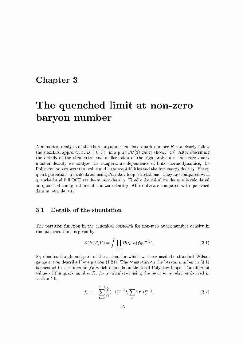
Chapter 3The quenched limit at non-zerobaryon numberA numerical analysis of the thermodynamics at �xed quark number B can closely followthe standard approach at B = 0, i.e. in a pure SU(3) gauge theory [48]. After describingthe details of the simulation and a discussion of the sign problem at non-zero quarknumber density we analyze the temperature dependence of bulk thermodynamics, thePolyakov loop expectation value and its susceptibilities and the free energy density. Heavyquark potentials are calculated using Polyakov loop correlations. They are compared withquenched and full QCD results at zero density. Finally the chiral condensate is calculatedon quenched con�gurations at non-zero density. All results are compared with quencheddata at zero density.3.1 Details of the simulationThe partition function in the canonical approach for non-zero quark number density inthe quenched limit is given byZ(B;T; V ) = Z Yn;� DU�(n)fBe�SG : (3.1)SG denotes the gluonic part of the action, for which we have used the standard Wilsongauge action described by equation (1.24). The constraint on the baryon number in (3.1)is encoded in the function fB which depends on the local Polyakov loops. For di�erentvalues of the quark number B, fB is calculated using the recurrence relation derived insection 1.9, fn = � n�1Xi=0 2n(�1)n�ifiX~x Tr P n�i~x : (3.2)43

44 Chapter 3. The quenched limit at non-zero baryon numberwith f0 = 1 and the symmetry fn = f�6V�n. P~x denotes the local Polyakov loop at site ~x.The expressions for some values of the quark number B are calculated section 1.9.The global Z(3) symmetry of the QCD partition function at non-zero quark number ispreserved also in the quenched limit, i.e. the function fB is invariant under global Z(3)transformations if B is a multiple of 3. As the gluonic action SG also shares this property,the partition function Z(B;T; V ) is non-zero only if B is a multiple of 3.The function fB is a complex valued function of the Polyakov loops, but when integratingover all gauge �elds in the canonical partition function (3.1), the contribution from theimaginary part of fB vanishes and the partition function is real, as it should be. Actualcalculations can thus be performed using the real part of fB. The sign problem thatremains in this formulation can be handled by shifting the dependence on the sign into theobservables and using a reweighting method [78] to calculate expectation values accordingto hOi = hO � sgn(RefB)ijjhsgn(RefB)ijj ; (3.3)where the expectation values h: : : ijj are calculated using the partition functionZjj(B;T; V ) = Z Yx;� DUx;�jRefBje�SG : (3.4)Our simulations were performed using a combination of a Metropolis update and over-relaxation steps to reduce autocorrelations. Each sweep consists of one Metropolis and fourover-relaxation steps. Measurements of the observables were performed after each sweep.For each link update the change in the function fB is calculated and a possible changein sign is monitored. The errors on observables were calculated using a Jackknife errorN3� �N� B nB=T 3 N3� �N� B nB=T 383 � 2 0 0.0000 83 � 4 6 0.250083 � 2 6 0.0313 103 � 4 6 0.128083 � 2 12 0.0625 123 � 4 6 0.0741103 � 2 0 0.0000 163 � 4 0 0.0000103 � 2 12 0.0320 163 � 4 6 0.0313163 � 4 12 0.0625Table 3.1: Lattice sizes and densities of the simula-tions.analysis with 10 Jackknife-blocks.Interpolations were performed us-ing the Ferrenberg Swendsenmethod.Our simulations have been carriedout in the vicinity of the criti-cal coupling for the decon�nementtransition at B = 0. Calcula-tions with �xed B were performedon lattices of size N3� � N� withN� = 2 and 4 and various val-ues for N�. The temperature isvaried by changing the coupling� = 6=g2. The temperature scales in our plots are set by a strong coupling expansionof the string tension [79] for the N� = 2 results, resp. by the �-function of [48] for N� = 4.The dimensionless parameter kept �xed in the simulation is the quark number density inunits of the temperature cubed, nBT 3 = B3 �N�N��3 : (3.5)

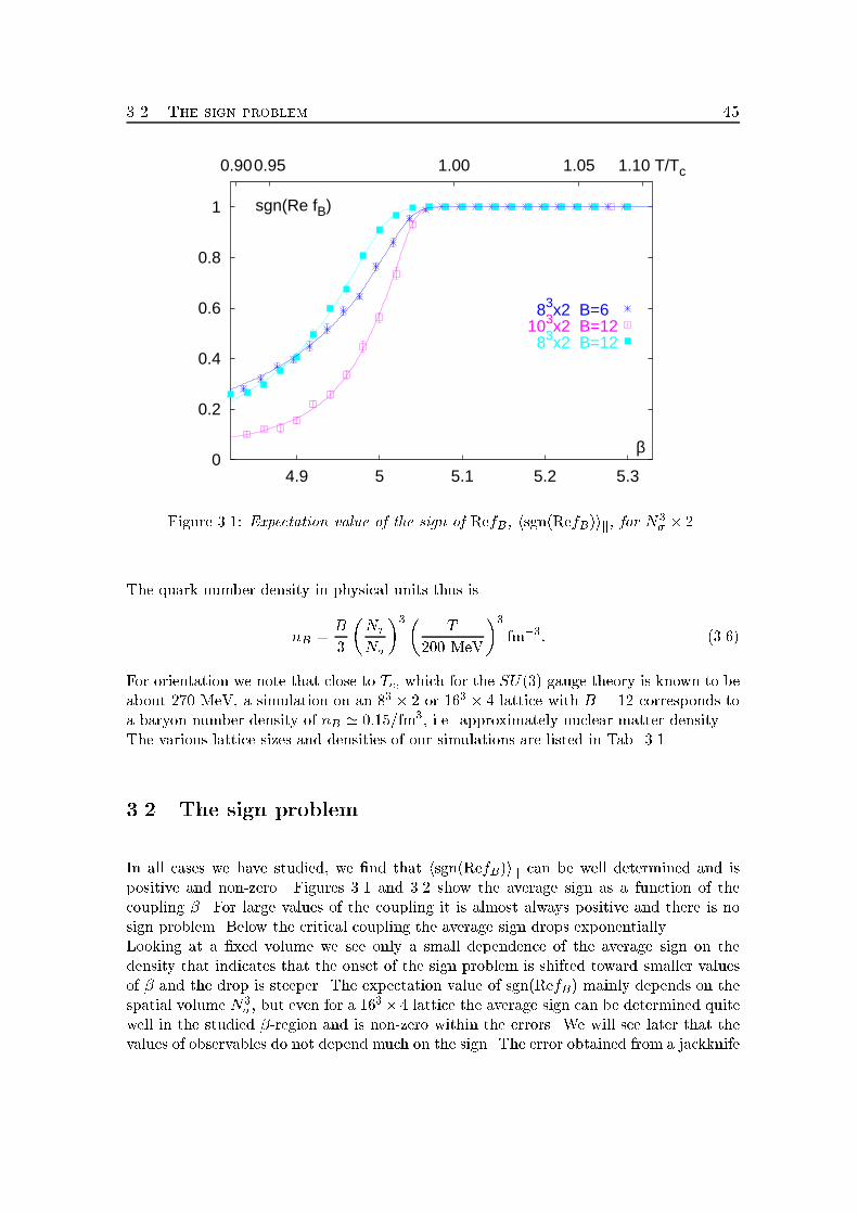
3.2. The sign problem 45

0

0.2

0.4

0.6

0.8

1

4.9 5 5.1 5.2 5.3

0.900.95 1.00 1.05 1.10 T/Tc

sgn(Re fB)

β

83x2 B=6 103x2 B=12 83x2 B=12

Figure 3.1: Expectation value of the sign of RefB, hsgn(RefB)ijj, for N3� � 2.The quark number density in physical units thus isnB = B3 �N�N��3� T200 MeV�3 fm�3: (3.6)For orientation we note that close to Tc, which for the SU(3) gauge theory is known to beabout 270 MeV, a simulation on an 83 � 2 or 163 � 4 lattice with B = 12 corresponds toa baryon number density of nB ' 0:15=fm3, i.e. approximately nuclear matter density.The various lattice sizes and densities of our simulations are listed in Tab. 3.1.3.2 The sign problemIn all cases we have studied, we �nd that hsgn(RefB)ijj can be well determined and ispositive and non-zero. Figures 3.1 and 3.2 show the average sign as a function of thecoupling �. For large values of the coupling it is almost always positive and there is nosign problem. Below the critical coupling the average sign drops exponentially.Looking at a �xed volume we see only a small dependence of the average sign on thedensity that indicates that the onset of the sign problem is shifted toward smaller valuesof � and the drop is steeper. The expectation value of sgn(RefB) mainly depends on thespatial volume N3� , but even for a 163� 4 lattice the average sign can be determined quitewell in the studied �-region and is non-zero within the errors. We will see later that thevalues of observables do not depend much on the sign. The error obtained from a jackknife

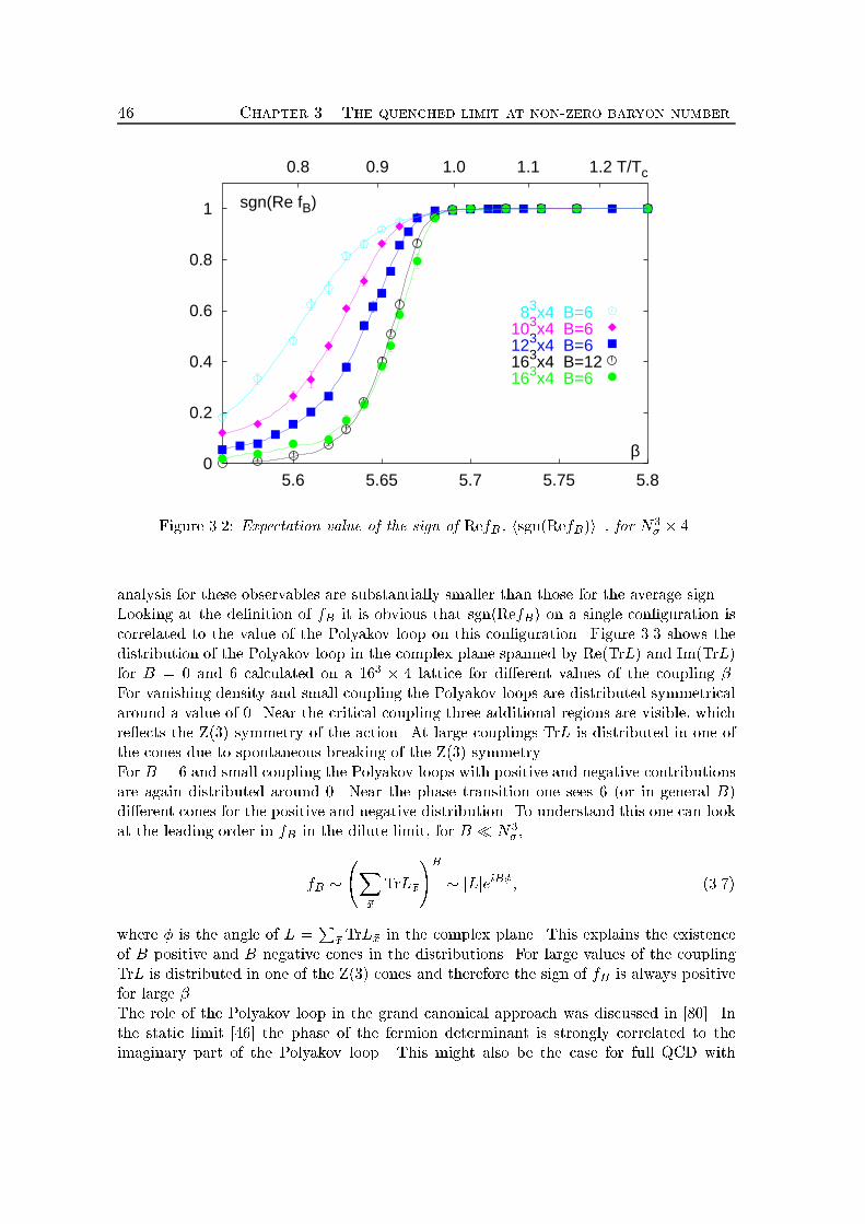
46 Chapter 3. The quenched limit at non-zero baryon number

0

0.2

0.4

0.6

0.8

1

5.6 5.65 5.7 5.75 5.8

0.8 0.9 1.0 1.1 1.2 T/Tc

sgn(Re fB)

β

83x4 B=6 103x4 B=6 123x4 B=6 163x4 B=12163x4 B=6

Figure 3.2: Expectation value of the sign of RefB, hsgn(RefB)ijj, for N3� � 4.analysis for these observables are substantially smaller than those for the average sign.Looking at the de�nition of fB it is obvious that sgn(RefB) on a single con�guration iscorrelated to the value of the Polyakov loop on this con�guration. Figure 3.3 shows thedistribution of the Polyakov loop in the complex plane spanned by Re(TrL) and Im(TrL)for B = 0 and 6 calculated on a 163 � 4 lattice for di�erent values of the coupling �.For vanishing density and small coupling the Polyakov loops are distributed symmetricalaround a value of 0. Near the critical coupling three additional regions are visible, whichre ects the Z(3) symmetry of the action. At large couplings TrL is distributed in one ofthe cones due to spontaneous breaking of the Z(3) symmetry.For B = 6 and small coupling the Polyakov loops with positive and negative contributionsare again distributed around 0. Near the phase transition one sees 6 (or in general B)di�erent cones for the positive and negative distribution. To understand this one can lookat the leading order in fB in the dilute limit, for B � N3� ,fB � X~x TrL~x!B � jLjeiB�; (3.7)where � is the angle of L = P~xTrL~x in the complex plane. This explains the existenceof B positive and B negative cones in the distributions. For large values of the couplingTrL is distributed in one of the Z(3) cones and therefore the sign of fB is always positivefor large �.The role of the Polyakov loop in the grand canonical approach was discussed in [80]. Inthe static limit [46] the phase of the fermion determinant is strongly correlated to theimaginary part of the Polyakov loop. This might also be the case for full QCD with

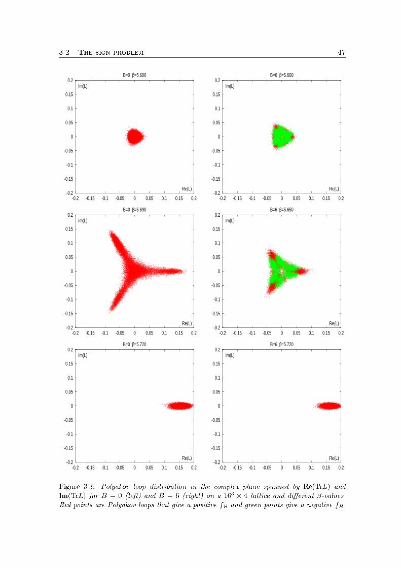
3.2. The sign problem 47

-0.2

-0.15

-0.1

-0.05

0

0.05

0.1

0.15

0.2

-0.2 -0.15 -0.1 -0.05 0 0.05 0.1 0.15 0.2

B=0 β=5.600

Re(L)

Im(L)

-0.2

-0.15

-0.1

-0.05

0

0.05

0.1

0.15

0.2

-0.2 -0.15 -0.1 -0.05 0 0.05 0.1 0.15 0.2

B=6 β=5.600

Re(L)

Im(L)

-0.2

-0.15

-0.1

-0.05

0

0.05

0.1

0.15

0.2

-0.2 -0.15 -0.1 -0.05 0 0.05 0.1 0.15 0.2

B=0 β=5.690

Re(L)

Im(L)

-0.2

-0.15

-0.1

-0.05

0

0.05

0.1

0.15

0.2

-0.2 -0.15 -0.1 -0.05 0 0.05 0.1 0.15 0.2

B=6 β=5.650

Re(L)

Im(L)

-0.2

-0.15

-0.1

-0.05

0

0.05

0.1

0.15

0.2

-0.2 -0.15 -0.1 -0.05 0 0.05 0.1 0.15 0.2

B=0 β=5.720

Re(L)

Im(L)

-0.2

-0.15

-0.1

-0.05

0

0.05

0.1

0.15

0.2

-0.2 -0.15 -0.1 -0.05 0 0.05 0.1 0.15 0.2

B=6 β=5.720

Re(L)

Im(L)

Figure 3.3: Polyakov loop distribution in the complex plane spanned by Re(TrL) andIm(TrL) for B = 0 (left) and B = 6 (right) on a 163 � 4 lattice and di�erent �-values.Red points are Polyakov loops that give a positive fB and green points give a negative fB.

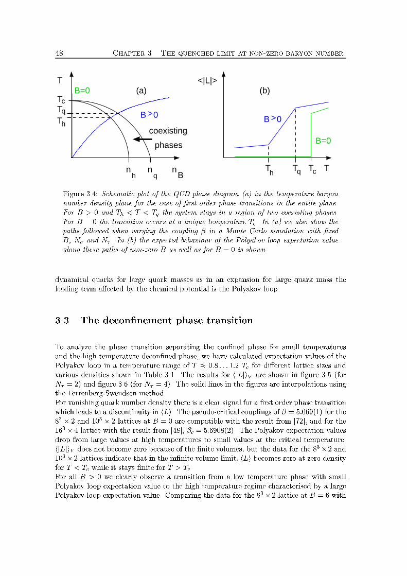
48 Chapter 3. The quenched limit at non-zero baryon numberB >0 >0

phases

B=0 (b)(a)<|L|>

Tqnqh

nn

T

B h c T

T

h

cq

T T

T

T

B=0

Bcoexisting

Figure 3.4: Schematic plot of the QCD phase diagram (a) in the temperature-baryonnumber density plane for the case of �rst order phase transitions in the entire plane.For B > 0 and Th < T < Tq the system stays in a region of two coexisting phases.For B = 0 the transition occurs at a unique temperature Tc. In (a) we also show thepaths followed when varying the coupling � in a Monte-Carlo simulation with �xedB, N� and N� . In (b) the expected behaviour of the Polyakov loop expectation valuealong these paths of non-zero B as well as for B = 0 is shown.dynamical quarks for large quark masses as in an expansion for large quark mass theleading term a�ected by the chemical potential is the Polyakov loop.3.3 The decon�nement phase transitionTo analyze the phase transition separating the con�ned phase for small temperaturesand the high temperature decon�ned phase, we have calculated expectation values of thePolyakov loop in a temperature range of T � 0:8 : : : 1:2 Tc for di�erent lattice sizes andvarious densities shown in Table 3.1. The results for hjLjiV are shown in �gure 3.5 (forN� = 2) and �gure 3.6 (for N� = 4). The solid lines in the �gures are interpolations usingthe Ferrenberg-Swendsen method.For vanishing quark number density there is a clear signal for a �rst order phase transitionwhich leads to a discontinuity in hLi. The pseudo-critical couplings of � = 5:069(1) for the83 � 2 and 103 � 2 lattices at B = 0 are compatible with the result from [72], and for the163 � 4 lattice with the result from [48], �c = 5:6908(2). The Polyakov expectation valuesdrop from large values at high temperatures to small values at the critical temperature.hjLjiV does not become zero because of the �nite volumes, but the data for the 83� 2 and103� 2 lattices indicate that in the in�nite volume limit, hLi becomes zero at zero densityfor T < Tc while it stays �nite for T > Tc.For all B > 0 we clearly observe a transition from a low temperature phase with smallPolyakov loop expectation value to the high temperature regime characterised by a largePolyakov loop expectation value. Comparing the data for the 83� 2 lattice at B = 6 with

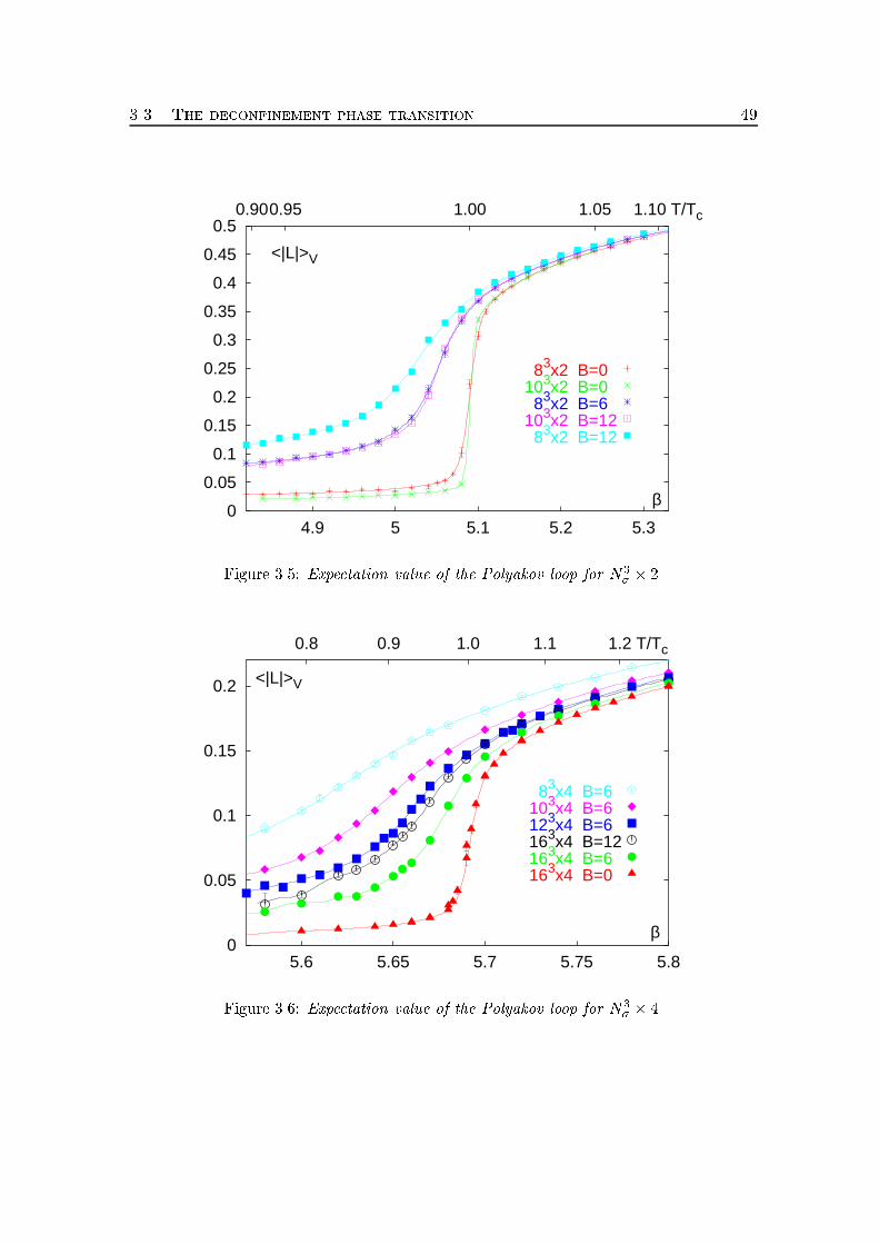
3.3. The deconfinement phase transition 49

0

0.05

0.1

0.15

0.2

0.25

0.3

0.35

0.4

0.45

0.5

4.9 5 5.1 5.2 5.3

0.900.95 1.00 1.05 1.10 T/Tc

β

<|L|>V

83x2 B=0 103x2 B=0 83x2 B=6 103x2 B=12 83x2 B=12

Figure 3.5: Expectation value of the Polyakov loop for N3� � 2.

0

0.05

0.1

0.15

0.2

5.6 5.65 5.7 5.75 5.8

0.8 0.9 1.0 1.1 1.2 T/Tc

β

<|L|>V

83x4 B=6 103x4 B=6 123x4 B=6 163x4 B=12163x4 B=6 163x4 B=0

Figure 3.6: Expectation value of the Polyakov loop for N3� � 4.

50 Chapter 3. The quenched limit at non-zero baryon numberthe 103 � 2 lattice at B = 12, which correspond to approximately the same density ofnB=T 3 = 0:0313 respectively 0:0320, we see no signi�cant volume dependence at �xed nB.This indicates that in the thermodynamic limit the physical observables will only dependon the density rather than on quark number and volume separately. It also indicates thatfor the small temperature regime the Polyakov loop hLi stays �nite for non-zero densitywhile it gets zero for vanishing density.For non-vanishing density the transition occurs in a temperature interval that broad-ens with increasing quark number density and gets shifted towards smaller temperatures.There is no indication for a discontinuous transition in contrast to the B = 0 case. Infact, this is the expected behaviour in a canonical calculation, even if the transition is of�rst order. By changing the gauge coupling � we vary the lattice cut-o� and through thisalso the quark number density continuously through a region of two coexisting phases.This situation is schematically illustrated in �gure 3.4. The question now is whether thetransition region really is a region of coexisting phases. In this case the values of thermo-dynamic observables result as the superposition of contributions from two di�erent phasesappropriately weighted by the fraction each phase contributes to the coexistence region(for an illustration see e.g. �gure 3.4b).To gain further insight into the structure of this regime we also analyze various suscepti-bilities. In �gures 3.7 and 3.8 we show the conventional Polyakov loop susceptibility,�L = N3� �hjLj2i � hjLji2� ; (3.8)and in �gures 3.9 and 3.10 the derivative of hjLji with respect to �,�� = @hjLji@� = N3� (hjLj � SGi � hjLjihSGi) : (3.9)Both response functions re ect the existence of a transition region that becomes broaderwith increasing nB and is shifted towards smaller temperatures. Compared to the be-haviour at B = 0 they also change continuously in this region. Such a behaviour might aswell just correspond to a smooth crossover to the high temperature regime; a conclusionalso drawn from the heavy quark simulations with non-zero chemical potential [46]. Toestablish the existence of a region of coexisting phases with certainty will thus require afurther, detailed analysis of �nite size e�ects.

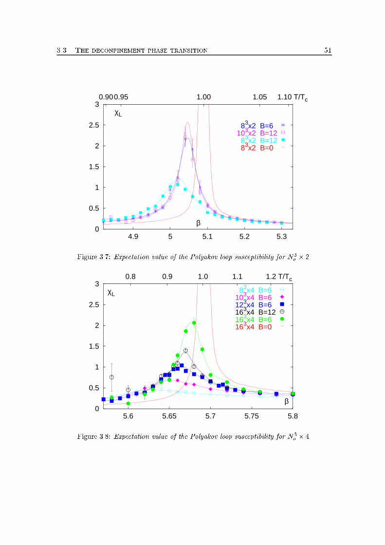
3.3. The deconfinement phase transition 51

0

0.5

1

1.5

2

2.5

3

4.9 5 5.1 5.2 5.3

0.900.95 1.00 1.05 1.10 T/Tc

β

χL

83x2 B=6 103x2 B=12 83x2 B=12 83x2 B=0

Figure 3.7: Expectation value of the Polyakov loop susceptibility for N3� � 2.

0

0.5

1

1.5

2

2.5

3

5.6 5.65 5.7 5.75 5.8

0.8 0.9 1.0 1.1 1.2 T/Tc

β

χL 83x4 B=6

103x4 B=6 123x4 B=6 163x4 B=12163x4 B=6 163x4 B=0

Figure 3.8: Expectation value of the Polyakov loop susceptibility for N3� � 4.

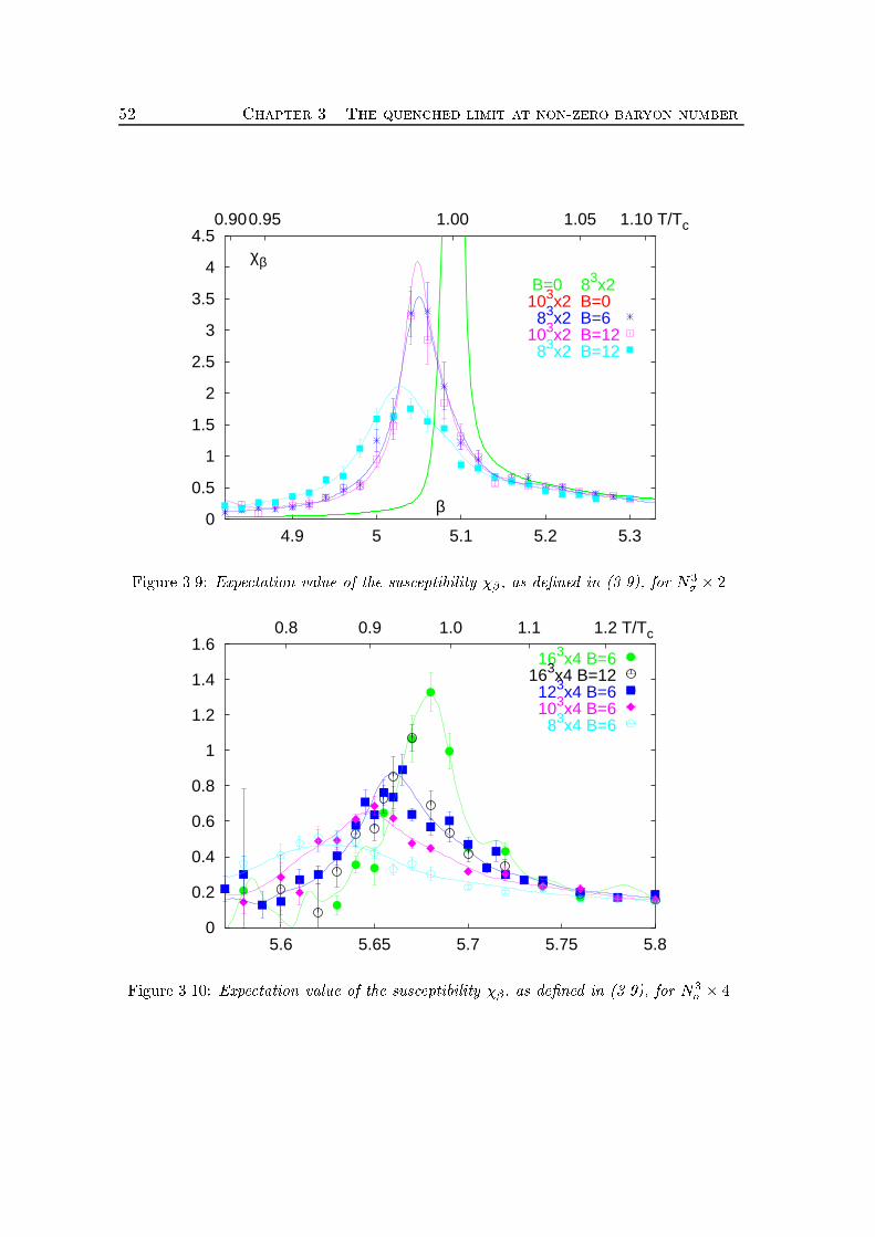
52 Chapter 3. The quenched limit at non-zero baryon number

0

0.5

1

1.5

2

2.5

3

3.5

4

4.5

4.9 5 5.1 5.2 5.3

0.900.95 1.00 1.05 1.10 T/Tc

β

χβ

B=0 83x2 103x2 B=0 83x2 B=6 103x2 B=12 83x2 B=12

Figure 3.9: Expectation value of the susceptibility ��, as de�ned in (3.9), for N3� � 2.

0

0.2

0.4

0.6

0.8

1

1.2

1.4

1.6

5.6 5.65 5.7 5.75 5.8

0.8 0.9 1.0 1.1 1.2 T/Tc

163x4 B=6163x4 B=12

123x4 B=6103x4 B=6 83x4 B=6

Figure 3.10: Expectation value of the susceptibility ��, as de�ned in (3.9), for N3� � 4.

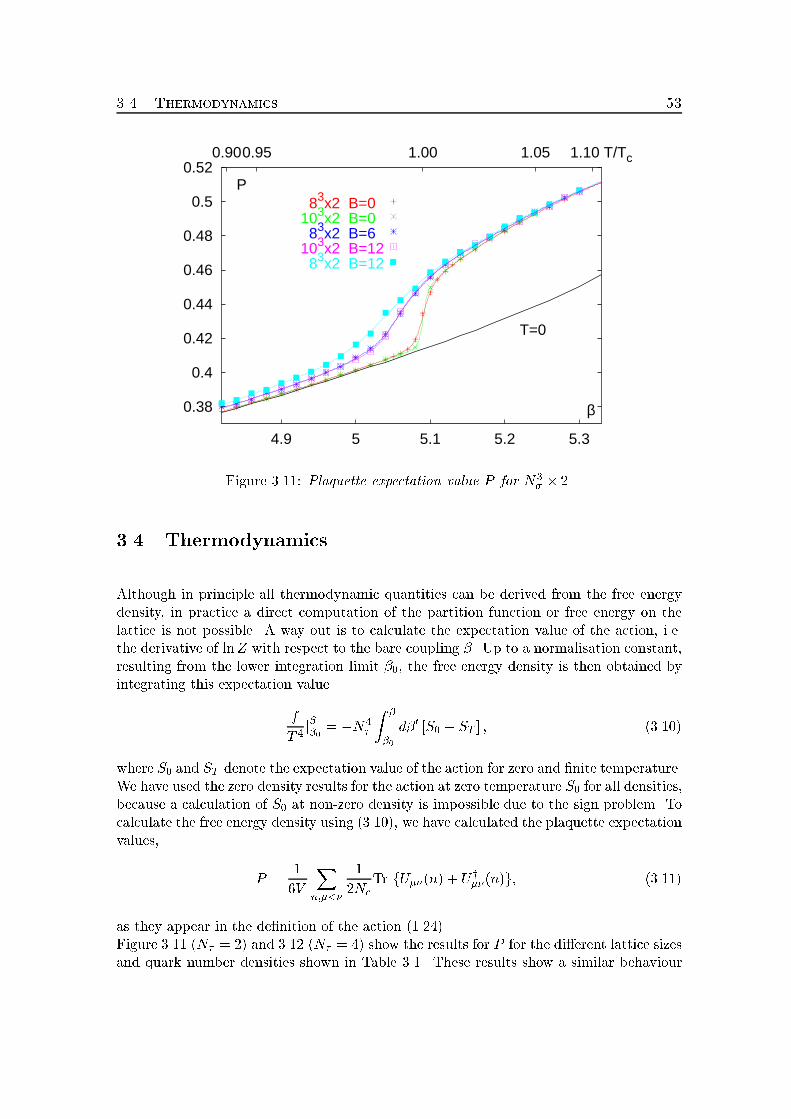
3.4. Thermodynamics 53

0.38

0.4

0.42

0.44

0.46

0.48

0.5

0.52

4.9 5 5.1 5.2 5.3

0.900.95 1.00 1.05 1.10 T/Tc

β

P

T=0

83x2 B=0 103x2 B=0 83x2 B=6 103x2 B=12 83x2 B=12

Figure 3.11: Plaquette expectation value P for N3� � 2.3.4 ThermodynamicsAlthough in principle all thermodynamic quantities can be derived from the free energydensity, in practice a direct computation of the partition function or free energy on thelattice is not possible. A way out is to calculate the expectation value of the action, i.e.the derivative of lnZ with respect to the bare coupling �. Up to a normalisation constant,resulting from the lower integration limit �0, the free energy density is then obtained byintegrating this expectation valuefT 4 j��0 = �N4� Z ��0 d�0 [S0 � ST ] ; (3.10)where S0 and ST denote the expectation value of the action for zero and �nite temperature.We have used the zero density results for the action at zero temperature S0 for all densities,because a calculation of S0 at non-zero density is impossible due to the sign problem. Tocalculate the free energy density using (3.10), we have calculated the plaquette expectationvalues, P = 16V Xn;�<� 12NcTr fU��(n) + U y��(n)g; (3.11)as they appear in the de�nition of the action (1.24).Figure 3.11 (N� = 2) and 3.12 (N� = 4) show the results for P for the di�erent lattice sizesand quark number densities shown in Table 3.1. These results show a similar behaviour

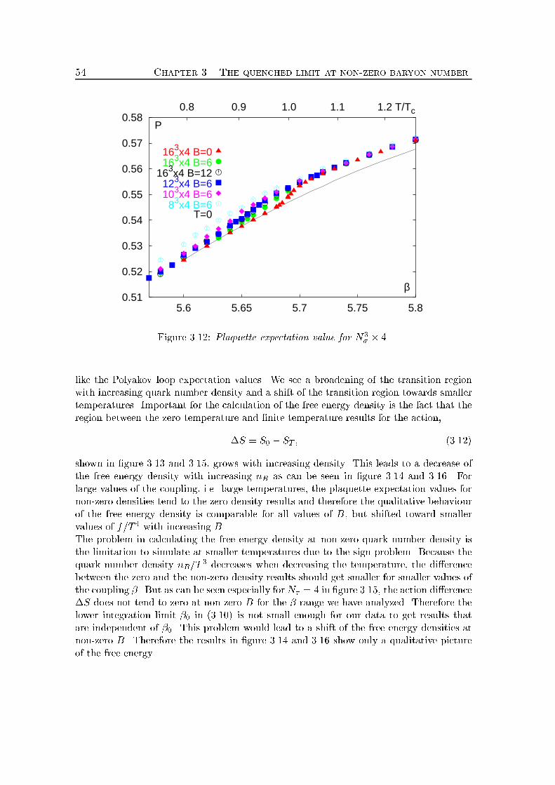
54 Chapter 3. The quenched limit at non-zero baryon number

0.51

0.52

0.53

0.54

0.55

0.56

0.57

0.58

5.6 5.65 5.7 5.75 5.8

0.8 0.9 1.0 1.1 1.2 T/Tc

β

P

163x4 B=0163x4 B=6

163x4 B=12123x4 B=6103x4 B=6 83x4 B=6

T=0

Figure 3.12: Plaquette expectation value for N3� � 4.like the Polyakov loop expectation values. We see a broadening of the transition regionwith increasing quark number density and a shift of the transition region towards smallertemperatures. Important for the calculation of the free energy density is the fact that theregion between the zero temperature and �nite temperature results for the action,�S = S0 � ST ; (3.12)shown in �gure 3.13 and 3.15, grows with increasing density. This leads to a decrease ofthe free energy density with increasing nB as can be seen in �gure 3.14 and 3.16. Forlarge values of the coupling, i.e. large temperatures, the plaquette expectation values fornon-zero densities tend to the zero density results and therefore the qualitative behaviourof the free energy density is comparable for all values of B, but shifted toward smallervalues of f=T 4 with increasing B.The problem in calculating the free energy density at non-zero quark number density isthe limitation to simulate at smaller temperatures due to the sign problem. Because thequark number density nB=T 3 decreases when decreasing the temperature, the di�erencebetween the zero and the non-zero density results should get smaller for smaller values ofthe coupling �. But as can be seen especially for N� = 4 in �gure 3.15, the action di�erence�S does not tend to zero at non-zero B for the �-range we have analyzed. Therefore thelower integration limit �0 in (3.10) is not small enough for our data to get results thatare independent of �0. This problem would lead to a shift of the free energy densities atnon-zero B. Therefore the results in �gure 3.14 and 3.16 show only a qualitative pictureof the free energy.

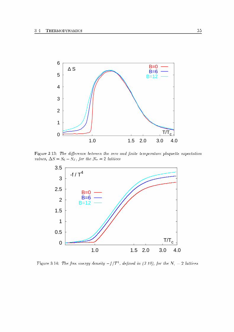
3.4. Thermodynamics 55

0

1

2

3

4

5

6

1.0 1.5 2.0 3.0 4.0

T/Tc

∆ S B=0B=6

B=12

Figure 3.13: The di�erence between the zero and �nite temperature plaquette expectationvalues, �S = S0 � ST , for the N� = 2 lattices.

0

0.5

1

1.5

2

2.5

3

3.5

1.0 1.5 2.0 3.0 4.0

T/Tc

-f / T4

B=0B=6

B=12

Figure 3.14: The free energy density �f=T 4, de�ned in (3.10), for the N� = 2 lattices.

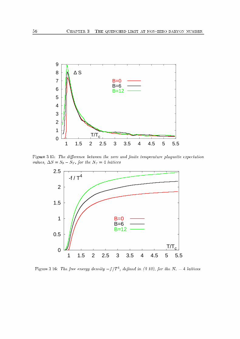
56 Chapter 3. The quenched limit at non-zero baryon number

0

1

2

3

4

5

6

7

8

9

1 1.5 2 2.5 3 3.5 4 4.5 5 5.5

T/Tc

∆ S

B=0 B=6 B=12

Figure 3.15: The di�erence between the zero and �nite temperature plaquette expectationvalues, �S = S0 � ST , for the N� = 4 lattices.

0

0.5

1

1.5

2

2.5

1 1.5 2 2.5 3 3.5 4 4.5 5 5.5

T/Tc

-f / T4

B=0 B=6 B=12

Figure 3.16: The free energy density �f=T 4, de�ned in (3.10), for the N� = 4 lattices.

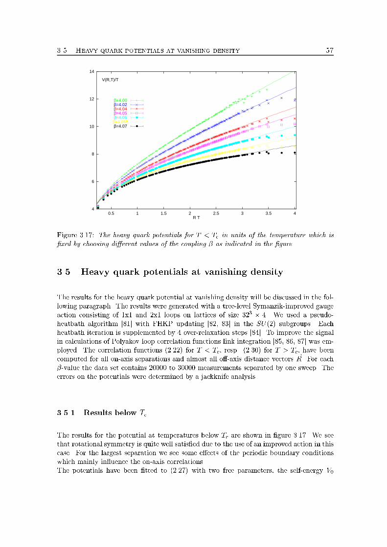
3.5. Heavy quark potentials at vanishing density 57

4

6

8

10

12

14

0.5 1 1.5 2 2.5 3 3.5 4R T

V(R,T)/T

β=4.00 β=4.02 β=4.04 β=4.05 β=4.06

β=4.065β=4.07

Figure 3.17: The heavy quark potentials for T < Tc in units of the temperature which is�xed by choosing di�erent values of the coupling � as indicated in the �gure.3.5 Heavy quark potentials at vanishing densityThe results for the heavy quark potential at vanishing density will be discussed in the fol-lowing paragraph. The results were generated with a tree-level Symanzik-improved gaugeaction consisting of 1x1 and 2x1 loops on lattices of size 323 � 4. We used a pseudo-heatbath algorithm [81] with FHKP updating [82, 83] in the SU(2) subgroups. Eachheatbath iteration is supplemented by 4 over-relaxation steps [84]. To improve the signalin calculations of Polyakov loop correlation functions link integration [85, 86, 87] was em-ployed. The correlation functions (2.22) for T < Tc, resp. (2.30) for T > Tc, have beencomputed for all on-axis separations and almost all o�-axis distance vectors ~R. For each�-value the data set contains 20000 to 30000 measurements separated by one sweep. Theerrors on the potentials were determined by a jackknife analysis.3.5.1 Results below TcThe results for the potential at temperatures below Tc are shown in �gure 3.17. We seethat rotational symmetry is quite well satis�ed due to the use of an improved action in thiscase. For the largest separation we see some e�ects of the periodic boundary conditionswhich mainly in uence the on-axis correlations.The potentials have been �tted to (2.27) with two free parameters, the self-energy V0

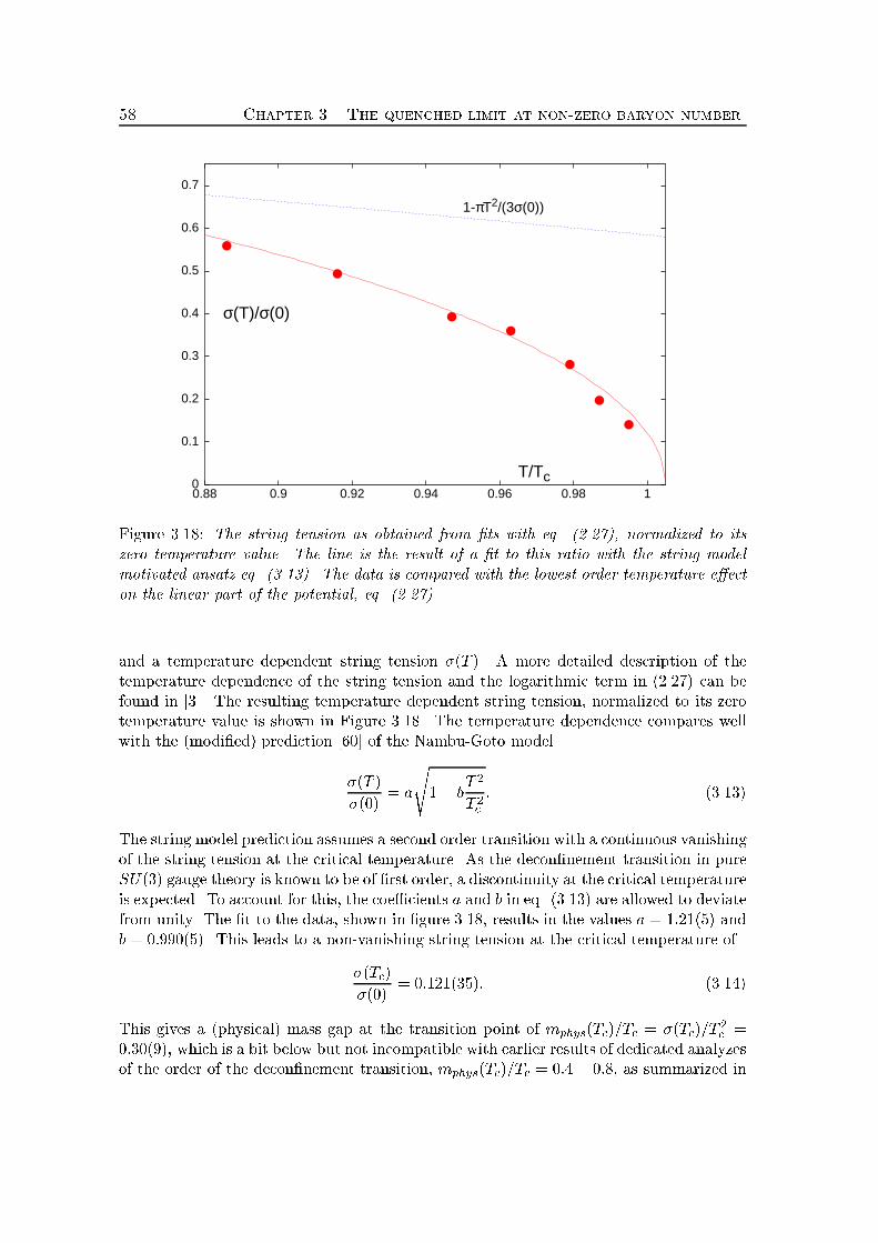
58 Chapter 3. The quenched limit at non-zero baryon number

0

0.1

0.2

0.3

0.4

0.5

0.6

0.7

0.88 0.9 0.92 0.94 0.96 0.98 1

σ(T)/σ(0)

1-πT2/(3σ(0))

T/TcFigure 3.18: The string tension as obtained from �ts with eq. (2.27), normalized to itszero temperature value. The line is the result of a �t to this ratio with the string modelmotivated ansatz eq. (3.13). The data is compared with the lowest order temperature e�ecton the linear part of the potential, eq. (2.27).and a temperature dependent string tension �(T ). A more detailed description of thetemperature dependence of the string tension and the logarithmic term in (2.27) can befound in [3]. The resulting temperature dependent string tension, normalized to its zerotemperature value is shown in Figure 3.18. The temperature dependence compares wellwith the (modi�ed) prediction [60] of the Nambu-Goto model�(T )�(0) = as1� bT 2T 2c : (3.13)The string model prediction assumes a second order transition with a continuous vanishingof the string tension at the critical temperature. As the decon�nement transition in pureSU(3) gauge theory is known to be of �rst order, a discontinuity at the critical temperatureis expected. To account for this, the coe�cients a and b in eq. (3.13) are allowed to deviatefrom unity. The �t to the data, shown in �gure 3.18, results in the values a = 1:21(5) andb = 0:990(5). This leads to a non-vanishing string tension at the critical temperature of�(Tc)�(0) = 0:121(35): (3.14)This gives a (physical) mass gap at the transition point of mphys(Tc)=Tc = �(Tc)=T 2c =0:30(9), which is a bit below but not incompatible with earlier results of dedicated analyzesof the order of the decon�nement transition, mphys(Tc)=Tc = 0:4� 0:8, as summarized in

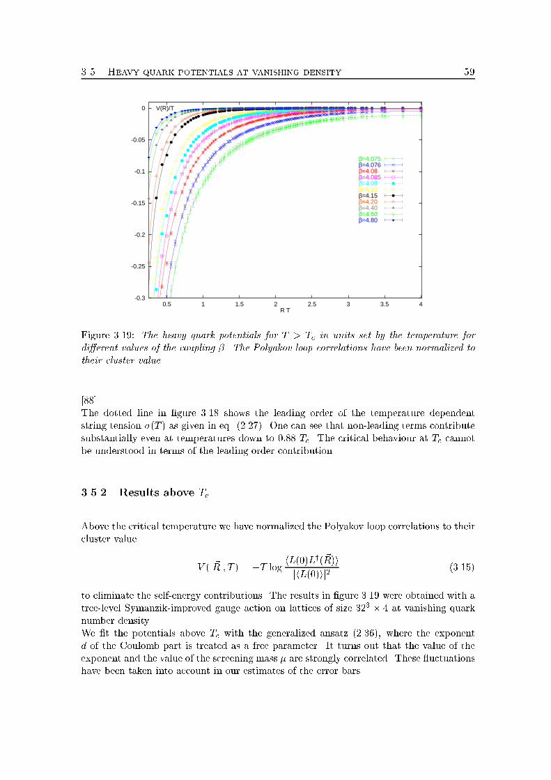
3.5. Heavy quark potentials at vanishing density 59

-0.3

-0.25

-0.2

-0.15

-0.1

-0.05

0

0.5 1 1.5 2 2.5 3 3.5 4R T

V(R)/T

β=4.075β=4.076β=4.08 β=4.085β=4.09 β=4.10 β=4.15 β=4.20 β=4.40 β=4.60 β=4.80

Figure 3.19: The heavy quark potentials for T > Tc in units set by the temperature fordi�erent values of the coupling �. The Polyakov loop correlations have been normalized totheir cluster value.[88].The dotted line in �gure 3.18 shows the leading order of the temperature dependentstring tension �(T ) as given in eq. (2.27). One can see that non-leading terms contributesubstantially even at temperatures down to 0:88 Tc. The critical behaviour at Tc cannotbe understood in terms of the leading order contribution.3.5.2 Results above TcAbove the critical temperature we have normalized the Polyakov loop correlations to theircluster value V (j~Rj; T ) = �T log hL(0)Ly(~R)ijhL(0)ij2 (3.15)to eliminate the self-energy contributions. The results in �gure 3.19 were obtained with atree-level Symanzik-improved gauge action on lattices of size 323 � 4 at vanishing quarknumber density.We �t the potentials above Tc with the generalized ansatz (2.36), where the exponentd of the Coulomb part is treated as a free parameter. It turns out that the value of theexponent and the value of the screening mass � are strongly correlated. These uctuationshave been taken into account in our estimates of the error bars.

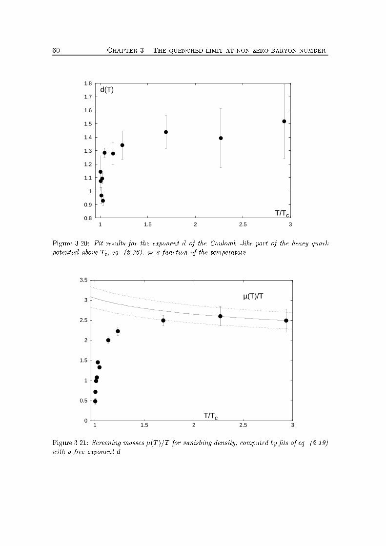
60 Chapter 3. The quenched limit at non-zero baryon number

0.8

0.9

1

1.1

1.2

1.3

1.4

1.5

1.6

1.7

1.8

1 1.5 2 2.5 3

T/Tc

d(T)

Figure 3.20: Fit results for the exponent d of the Coulomb -like part of the heavy quarkpotential above Tc, eq. (2.36), as a function of the temperature.

0

0.5

1

1.5

2

2.5

3

3.5

1 1.5 2 2.5 3

µ(T)/T

T/TcFigure 3.21: Screening masses �(T )=T for vanishing density, computed by �ts of eq. (2.19)with a free exponent d.

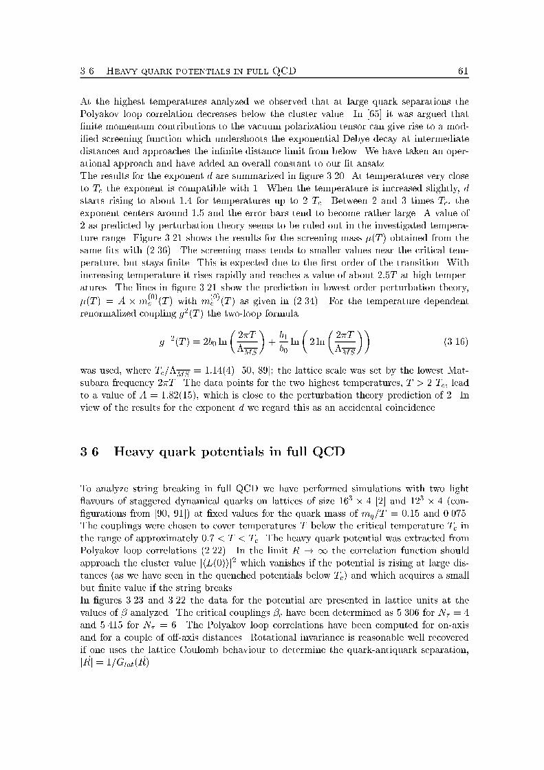
3.6. Heavy quark potentials in full QCD 61At the highest temperatures analyzed we observed that at large quark separations thePolyakov loop correlation decreases below the cluster value. In [65] it was argued that�nite momentum contributions to the vacuum polarization tensor can give rise to a mod-i�ed screening function which undershoots the exponential Debye decay at intermediatedistances and approaches the in�nite distance limit from below. We have taken an oper-ational approach and have added an overall constant to our �t ansatz.The results for the exponent d are summarized in �gure 3.20. At temperatures very closeto Tc the exponent is compatible with 1. When the temperature is increased slightly, dstarts rising to about 1:4 for temperatures up to 2 Tc. Between 2 and 3 times Tc, theexponent centers around 1:5 and the error bars tend to become rather large. A value of2 as predicted by perturbation theory seems to be ruled out in the investigated tempera-ture range. Figure 3.21 shows the results for the screening mass �(T ) obtained from thesame �ts with (2.36). The screening mass tends to smaller values near the critical tem-perature, but stays �nite. This is expected due to the �rst order of the transition. Withincreasing temperature it rises rapidly and reaches a value of about 2:5T at high temper-atures. The lines in �gure 3.21 show the prediction in lowest order perturbation theory,�(T ) = A � m(0)e (T ) with m(0)e (T ) as given in (2.34). For the temperature dependentrenormalized coupling g2(T ) the two-loop formulag�2(T ) = 2b0 ln� 2�T�MS�+ b1b0 ln� 2 ln� 2�T�MS�� (3.16)was used, where Tc=�MS = 1:14(4) [50, 89]; the lattice scale was set by the lowest Mat-subara frequency 2�T . The data points for the two highest temperatures, T > 2 Tc, leadto a value of A = 1:82(15), which is close to the perturbation theory prediction of 2. Inview of the results for the exponent d we regard this as an accidental coincidence.3.6 Heavy quark potentials in full QCDTo analyze string breaking in full QCD we have performed simulations with two light avours of staggered dynamical quarks on lattices of size 163 � 4 [2] and 123 � 4 (con-�gurations from [90, 91]) at �xed values for the quark mass of mq=T = 0:15 and 0.075.The couplings were chosen to cover temperatures T below the critical temperature Tc inthe range of approximately 0:7 < T < Tc. The heavy quark potential was extracted fromPolyakov loop correlations (2.22). In the limit R ! 1 the correlation function shouldapproach the cluster value jhL(0)ij2 which vanishes if the potential is rising at large dis-tances (as we have seen in the quenched potentials below Tc) and which acquires a smallbut �nite value if the string breaks.In �gures 3.23 and 3.22 the data for the potential are presented in lattice units at thevalues of � analyzed. The critical couplings �c have been determined as 5.306 for N� = 4and 5.415 for N� = 6. The Polyakov loop correlations have been computed for on-axisand for a couple of o�-axis distances. Rotational invariance is reasonable well recoveredif one uses the lattice Coulomb behaviour to determine the quark-antiquark separation,j~Rj = 1=Glat(~R).

62 Chapter 3. The quenched limit at non-zero baryon number

1

1.5

2

2.5

3

0 1 2 3 4 5 6 7 8 9 10

V a

R / a

β = 5.10

1

1.2

1.4

1.6

1.8

2

2.2

2.4

2.6

0 1 2 3 4 5 6 7 8 9 10

V a

R / a

β = 5.20

1

1.2

1.4

1.6

1.8

2

2.2

0 1 2 3 4 5 6 7 8 9 10

V a

R / a

β = 5.25

1

1.2

1.4

1.6

1.8

2

0 1 2 3 4 5 6 7 8 9 10

V a

R / a

β = 5.28

Figure 3.22: Heavy quark potentials in lattice unites for staggered fermions and N� = 4.The right-most data points plotted at R=a = 9:5 and denoted by stars are the in�nitedistance cluster values �T ln jhLij2.The data quite clearly show a attening of the potential at lattice distances of about 3 ro4 lattice spacings, depending on �. This is in agreement with earlier results [92, 68] onsmaller lattices of size 83 � 4. Moreover, the height of the potential at these distances isin nice agreement already with the in�nite distance cluster value, shown as the right-mostdata point in each of the plots.In �gure 3.24 quenched [3] and full QCD [2] potentials are compared. In order to obtaina rough estimate of the corresponding temperatures in units of the critical temperature,the vector meson mass mV a as well as the ratio of pseudoscalar to vector meson mass,mPS=mV were estimated. The absolute scale was determined from conventional Wilsonloop measurements of the string tension at zero temperatures at the critical �c values.The dashed line denotes �=(12R) + (420MeV)2R which gives a good description of thezero temperature quenched potential. Again, the comparison with quenched potentialsat the same temperature demonstrates that the potential in the presence of dynamicalquarks becomes at within the error bars at distances of about 1 fm. From �gure 3.24

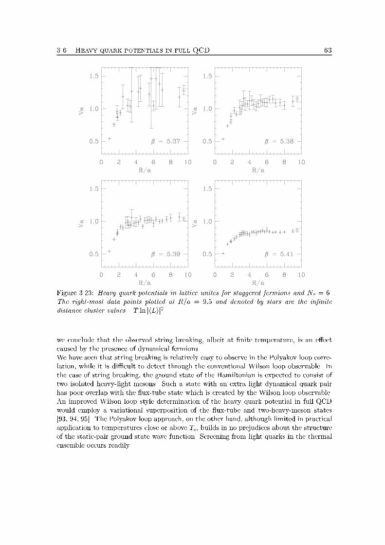
3.6. Heavy quark potentials in full QCD 63

Figure 3.23: Heavy quark potentials in lattice unites for staggered fermions and N� = 6.The right-most data points plotted at R=a = 9:5 and denoted by stars are the in�nitedistance cluster values �T ln jhLij2.we conclude that the observed string breaking, albeit at �nite temperature, is an e�ectcaused by the presence of dynamical fermions.We have seen that string breaking is relatively easy to observe in the Polyakov loop corre-lation, while it is di�cult to detect through the conventional Wilson loop observable. Inthe case of string breaking, the ground state of the Hamiltonian is expected to consist oftwo isolated heavy-light mesons. Such a state with an extra light dynamical quark pairhas poor overlap with the ux-tube state which is created by the Wilson loop observable.An improved Wilson loop style determination of the heavy quark potential in full QCDwould employ a variational superposition of the ux-tube and two-heavy-meson states[93, 94, 95]. The Polyakov loop approach, on the other hand, although limited in practicalapplication to temperatures close or above Tc, builds in no prejudices about the structureof the static-pair ground state wave function. Screening from light quarks in the thermalensemble occurs readily.

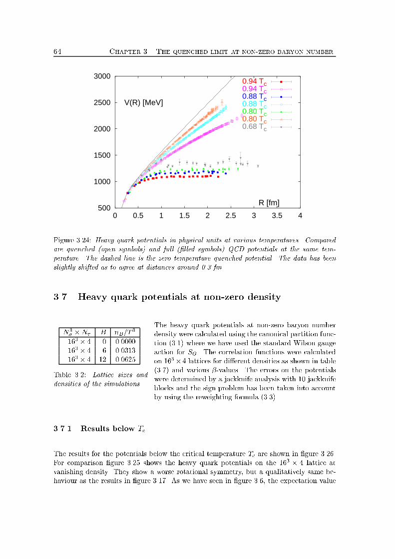
64 Chapter 3. The quenched limit at non-zero baryon number

500

1000

1500

2000

2500

3000

0 0.5 1 1.5 2 2.5 3 3.5 4

R [fm]

V(R) [MeV]

0.94 Tc0.94 Tc0.88 Tc0.88 Tc0.80 Tc0.80 Tc0.68 Tc

Figure 3.24: Heavy quark potentials in physical units at various temperatures. Comparedare quenched (open symbols) and full (�lled symbols) QCD potentials at the same tem-perature. The dashed line is the zero temperature quenched potential. The data has beenslightly shifted as to agree at distances around 0.3 fm.3.7 Heavy quark potentials at non-zero densityN3� �N� B nB=T 3163 � 4 0 0.0000163 � 4 6 0.0313163 � 4 12 0.0625Table 3.2: Lattice sizes anddensities of the simulations.The heavy quark potentials at non-zero baryon numberdensity were calculated using the canonical partition func-tion (3.1) where we have used the standard Wilson gaugeaction for SG. The correlation functions were calculatedon 163� 4 lattices for di�erent densities as shown in table(3.7) and various �-values. The errors on the potentialswere determined by a jackknife analysis with 10 jackknifeblocks and the sign problem has been taken into accountby using the reweighting formula (3.3).3.7.1 Results below TcThe results for the potentials below the critical temperature Tc are shown in �gure 3.26.For comparison �gure 3.25 shows the heavy quark potentials on the 163 � 4 lattice atvanishing density. They show a worse rotational symmetry, but a qualitatively same be-haviour as the results in �gure 3.17. As we have seen in �gure 3.6, the expectation value

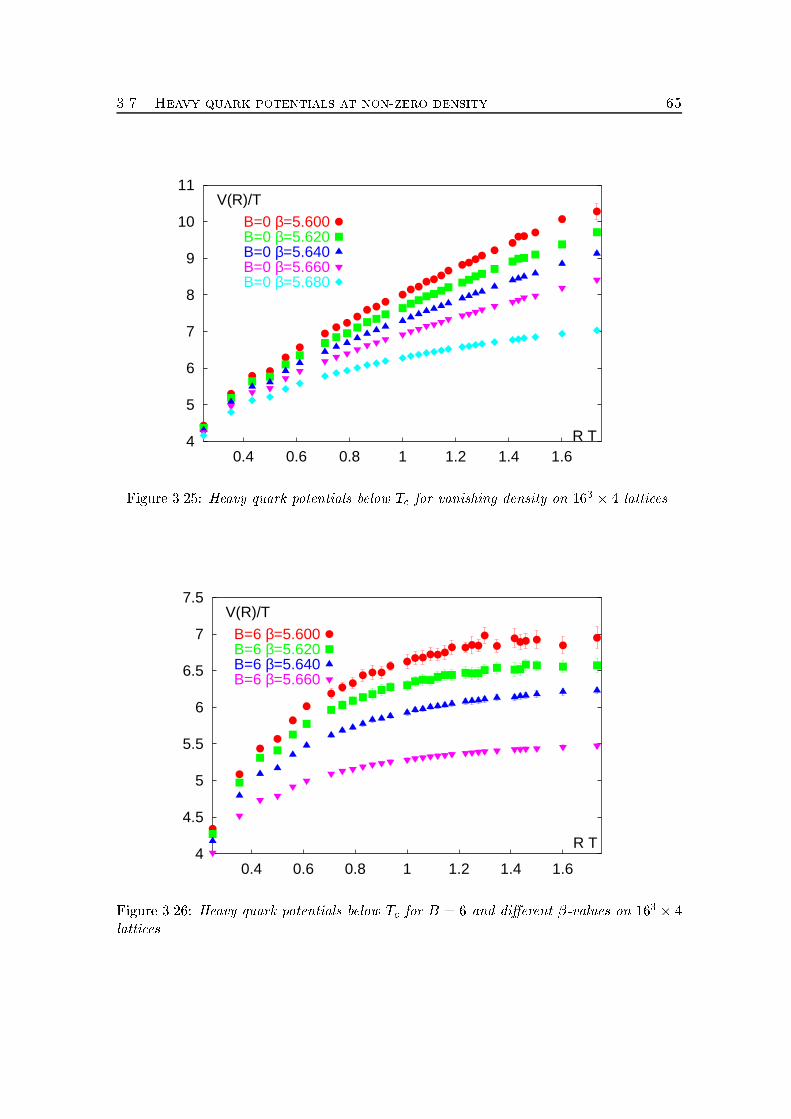
3.7. Heavy quark potentials at non-zero density 65

4

5

6

7

8

9

10

11

0.4 0.6 0.8 1 1.2 1.4 1.6

V(R)/T

R T

B=0 β=5.600B=0 β=5.620B=0 β=5.640B=0 β=5.660B=0 β=5.680

Figure 3.25: Heavy quark potentials below Tc for vanishing density on 163 � 4 lattices.

4

4.5

5

5.5

6

6.5

7

7.5

0.4 0.6 0.8 1 1.2 1.4 1.6

V(R)/T

R T

B=6 β=5.600B=6 β=5.620B=6 β=5.640B=6 β=5.660

Figure 3.26: Heavy quark potentials below Tc for B = 6 and di�erent �-values on 163 � 4lattices.

66 Chapter 3. The quenched limit at non-zero baryon number

4

5

6

7

8

9

10

0.4 0.6 0.8 1 1.2 1.4 1.6

V(R,T)/T

R T

163x4 B=0 163x4 B=6 163x4 B=12

Figure 3.27: Heavy quark potentials below Tc for � = 5:620 and di�erent densities on163 � 4 lattices.of the Polyakov loop stays non-zero for �nite baryon number density even for tempera-tures below the phase transition. In the limit of in�nite separation the potential can beexpressed in terms of the Polyakov loop expectation value (2.16). Therefore we expectthat the potential stays constant at large separations for nB=T 3 > 0. In �gure 3.26 wesee exactly this behaviour. For small separations the usual (quenched) behaviour can beidenti�ed and is comparable to the potentials in �gures 3.17 and 3.25. For larger distancesthe potential gets screened and stays constant in the limit of in�nite separations. Thismodi�cation of the long distance part of the heavy quark potential can be explained by thenon-zero density of heavy quarks on the lattice. The static quark anti-quark source usedto probe the potential can recombine with the already present static quarks on the lattice,forming a baryon and a meson, and therefore the potential gets screened. In �gure 3.27the potentials for � = 5:620 and the densities described in table (3.7) are shown. Withincreasing quark number density the screening of the heavy quark potential is increasedand the plateau where the potential stays constant gets smaller.Although the mechanism which leads to a breaking of the string is di�erent for thequenched case at non-zero density compared to the full QCD case discussed in section 3.6,the heavy quark potentials show a quite similar behaviour. For small separations theyare comparable with the quenched case, while at some distance R the string breaks andthe potential stays constant for large separations. While in the full QCD case a quarkanti-quark pair has to be created out of the vacuum to break the string, in the case ofnon-zero density the quarks are already present and at large separation it is energeticallyfavourable that the string breaks.

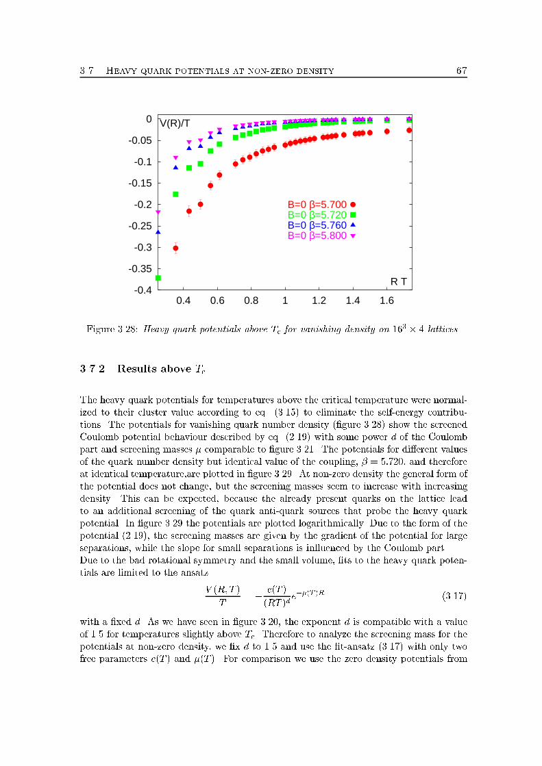
3.7. Heavy quark potentials at non-zero density 67

-0.4

-0.35

-0.3

-0.25

-0.2

-0.15

-0.1

-0.05

0

0.4 0.6 0.8 1 1.2 1.4 1.6

V(R)/T

R T

B=0 β=5.700B=0 β=5.720B=0 β=5.760B=0 β=5.800

Figure 3.28: Heavy quark potentials above Tc for vanishing density on 163 � 4 lattices.3.7.2 Results above TcThe heavy quark potentials for temperatures above the critical temperature were normal-ized to their cluster value according to eq. (3.15) to eliminate the self-energy contribu-tions. The potentials for vanishing quark number density (�gure 3.28) show the screenedCoulomb potential behaviour described by eq. (2.19) with some power d of the Coulombpart and screening masses � comparable to �gure 3.21. The potentials for di�erent valuesof the quark number density but identical value of the coupling, � = 5:720, and thereforeat identical temperature,are plotted in �gure 3.29. At non-zero density the general form ofthe potential does not change, but the screening masses seem to increase with increasingdensity. This can be expected, because the already present quarks on the lattice leadto an additional screening of the quark anti-quark sources that probe the heavy quarkpotential. In �gure 3.29 the potentials are plotted logarithmically. Due to the form of thepotential (2.19), the screening masses are given by the gradient of the potential for largeseparations, while the slope for small separations is in uenced by the Coulomb part.Due to the bad rotational symmetry and the small volume, �ts to the heavy quark poten-tials are limited to the ansatzV (R;T )T = � e(T )(RT )d e��(T )R (3.17)with a �xed d. As we have seen in �gure 3.20, the exponent d is compatible with a valueof 1.5 for temperatures slightly above Tc. Therefore to analyze the screening mass for thepotentials at non-zero density, we �x d to 1.5 and use the �t-ansatz (3.17) with only twofree parameters e(T ) and �(T ). For comparison we use the zero density potentials from

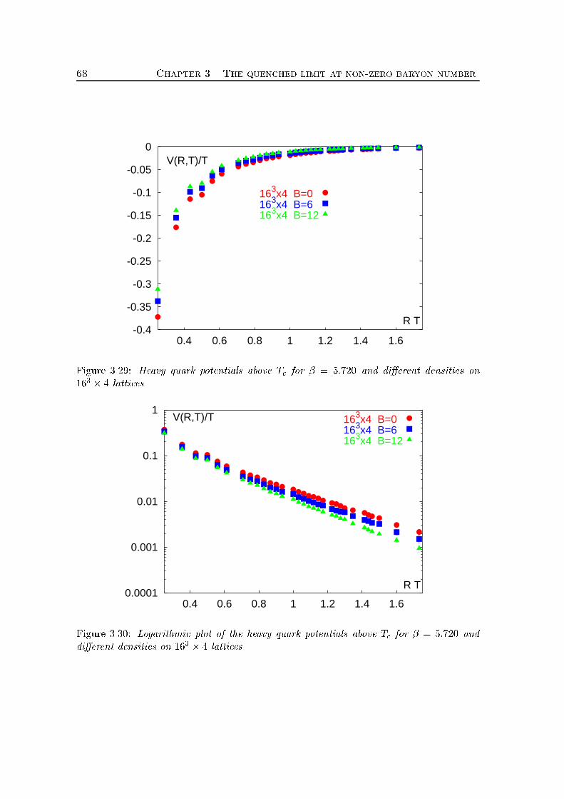
68 Chapter 3. The quenched limit at non-zero baryon number

-0.4

-0.35

-0.3

-0.25

-0.2

-0.15

-0.1

-0.05

0

0.4 0.6 0.8 1 1.2 1.4 1.6

V(R,T)/T

R T

163x4 B=0 163x4 B=6 163x4 B=12

Figure 3.29: Heavy quark potentials above Tc for � = 5:720 and di�erent densities on163 � 4 lattices.

0.0001

0.001

0.01

0.1

1

0.4 0.6 0.8 1 1.2 1.4 1.6

V(R,T)/T

R T

163x4 B=0 163x4 B=6 163x4 B=12

Figure 3.30: Logarithmic plot of the heavy quark potentials above Tc for � = 5:720 anddi�erent densities on 163 � 4 lattices.

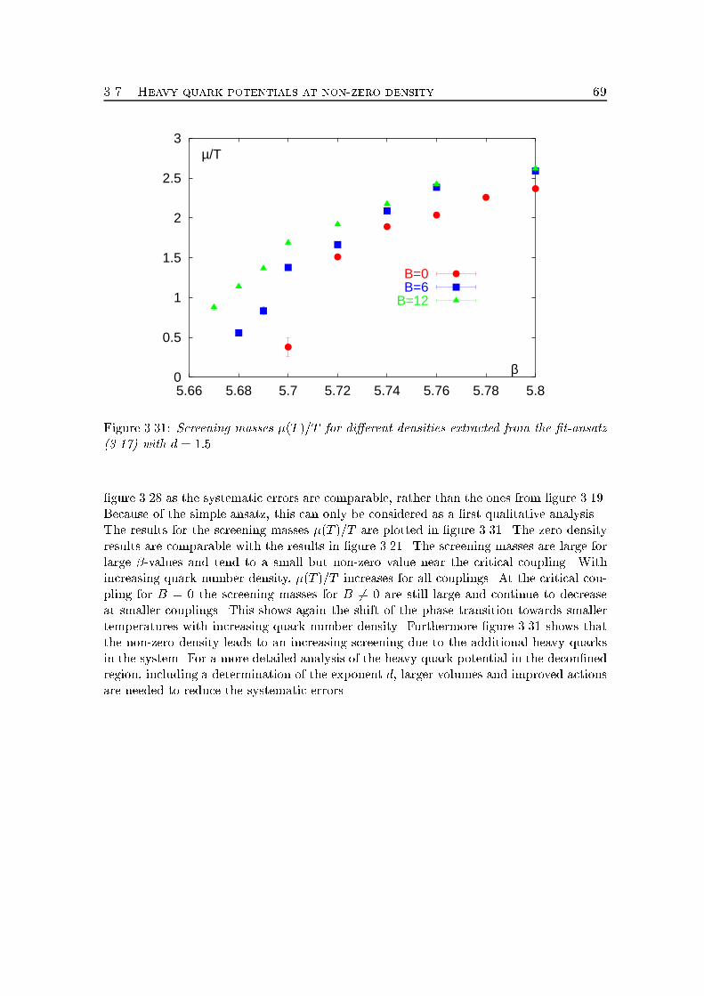
3.7. Heavy quark potentials at non-zero density 69

0

0.5

1

1.5

2

2.5

3

5.66 5.68 5.7 5.72 5.74 5.76 5.78 5.8

µ/T

β

B=0B=6

B=12

Figure 3.31: Screening masses �(T )=T for di�erent densities extracted from the �t-ansatz(3.17) with d = 1:5.�gure 3.28 as the systematic errors are comparable, rather than the ones from �gure 3.19.Because of the simple ansatz, this can only be considered as a �rst qualitative analysis.The results for the screening masses �(T )=T are plotted in �gure 3.31. The zero densityresults are comparable with the results in �gure 3.21. The screening masses are large forlarge �-values and tend to a small but non-zero value near the critical coupling. Withincreasing quark number density, �(T )=T increases for all couplings. At the critical cou-pling for B = 0 the screening masses for B 6= 0 are still large and continue to decreaseat smaller couplings. This shows again the shift of the phase transition towards smallertemperatures with increasing quark number density. Furthermore �gure 3.31 shows thatthe non-zero density leads to an increasing screening due to the additional heavy quarksin the system. For a more detailed analysis of the heavy quark potential in the decon�nedregion, including a determination of the exponent d, larger volumes and improved actionsare needed to reduce the systematic errors.

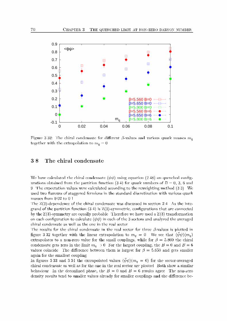
70 Chapter 3. The quenched limit at non-zero baryon number

-0.1

0

0.1

0.2

0.3

0.4

0.5

0.6

0.7

0.8

0.9

0 0.02 0.04 0.06 0.08 0.1

mq

<ψψ>--

β=5.560 B=0β=5.650 B=0β=5.800 B=0β=5.560 B=6β=5.650 B=6β=5.800 B=6Figure 3.32: The chiral condensate for di�erent �-values and various quark masses mqtogether with the extrapolation to mq = 0.3.8 The chiral condensateWe have calculated the chiral condensate h � i using equation (2.48) on quenched con�g-urations obtained from the partition function (3.4) for quark numbers of B = 0, 3, 6 and9. The expectation values were calculated according to the reweighting method (3.3). Weused two avours of staggered fermions in the standard discretization with various quarkmasses from 0.02 to 0.1.The Z(3)-dependence of the chiral condensate was discussed in section 2.4. As the inte-grand of the partition function (3.4) is Z(3)-symmetric, con�gurations that are connectedby the Z(3)-symmetry are equally probable. Therefore we have used a Z(3) transformationon each con�guration to calculate h � i in each of the 3 sectors and analyzed the averagedchiral condensate as well as the one in the real sector.The results for the chiral condensate in the real sector for three �-values is plotted in�gure 3.32 together with the linear extrapolation to mq = 0. We see that h � i(mq)extrapolates to a non-zero value for the small couplings, while for � = 5:800 the chiralcondensate gets zero in the limit mq ! 0. For the largest coupling, the B = 0 and B = 6values coincide. The di�erence between them is largest for � = 5:650 and gets smalleragain for the smallest coupling.In �gures 3.33 and 3.34 the extrapolated values h � i(mq = 0) for the sector-averagedchiral condensate as well as for the one in the real sector are plotted. Both show a similarbehaviour. In the decon�ned phase, the B = 0 and B = 6 results agree. The non-zerodensity results tend to smaller values already for smaller couplings and the di�erence be-

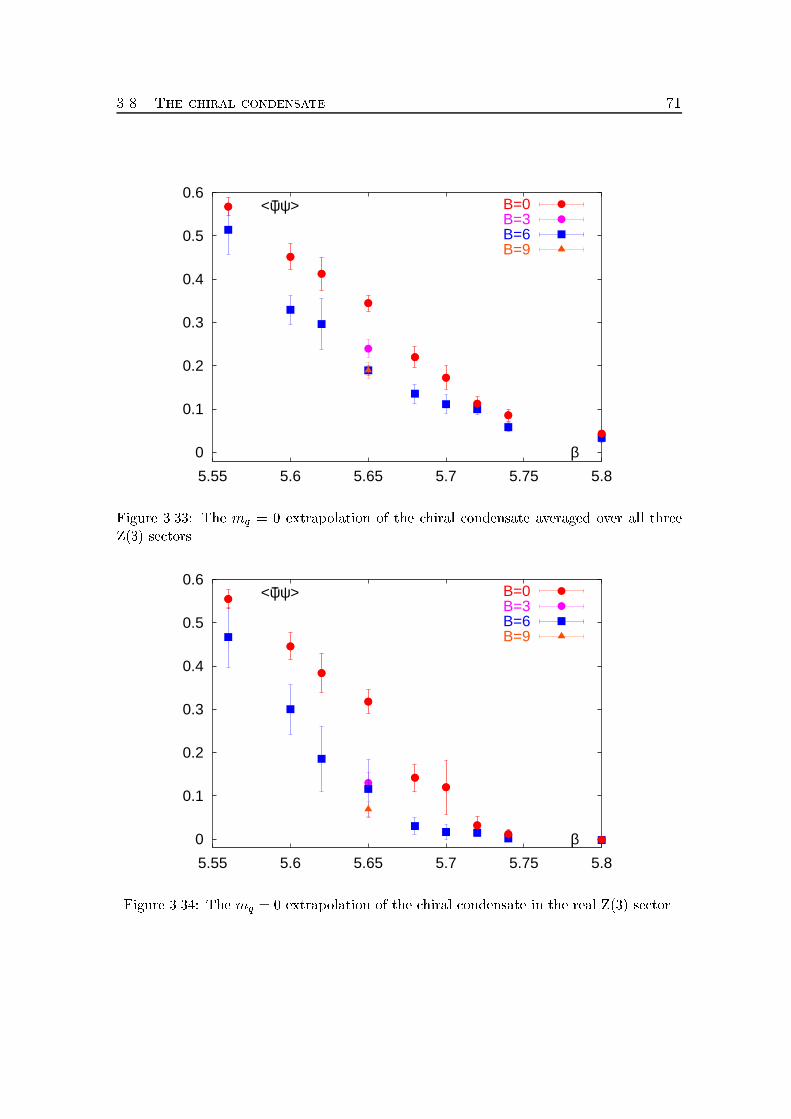
3.8. The chiral condensate 71

0

0.1

0.2

0.3

0.4

0.5

0.6

5.55 5.6 5.65 5.7 5.75 5.8

<ψψ>

β

-- B=0B=3B=6B=9

Figure 3.33: The mq = 0 extrapolation of the chiral condensate averaged over all threeZ(3) sectors.

0

0.1

0.2

0.3

0.4

0.5

0.6

5.55 5.6 5.65 5.7 5.75 5.8

<ψψ>

β

-- B=0B=3B=6B=9

Figure 3.34: The mq = 0 extrapolation of the chiral condensate in the real Z(3) sector.

72 Chapter 3. The quenched limit at non-zero baryon numbertween the zero and non-zero density values seem to be largest in the transition region. Forsmaller values of � they seem to get together again.The chiral condensates in �gures 3.33 and 3.34 mainly di�er in the vicinity and abovethe phase transition. For the smallest coupling they agree within errors. While the chi-ral condensate calculated in only the real sector extrapolates to zero for � = 5:80 forboth densities, it stays non-zero for the sector-averaged condensate. The behaviour forthe quenched chiral condensate for vanishing density in [73, 74] suggests that for largercouplings both methods should give the same result. Therefore we expect that also theaveraged condensate extrapolates to zero for larger �-values.

Chapter 4The quenched limit in the grandcanonical approachIn this chapter we discuss the results obtained for the grand canonical approach of latticeQCD in the quenched limit. After describing the details of the simulation and a discussionof the sign problem at non-zero chemical potential we analyze the temperature dependenceof bulk thermodynamics, the Polyakov loop expectation value and its susceptibility aswell as baryon number density. All results are compared with the results of the canonicalapproach discussed in the previous chapter. We will also discuss the possibility of a criticalendpoint of the �rst order phase transition and analyze its properties.4.1 Details of the simulationThe simulations for the grand canonical approach in the limit of static quarks, i.e. thelimit �!1 and �! 0, keeping �e� �xed, were performed with the partition functionZgc = Z dU jRe(det(M))je�SG ; (4.1)where det(M) is the quenched limit of the fermion determinant in the Wilson formulation,as derived in section 1.9,det(M) = Y~x �det�P y~x + C�1��2= Y~x �C�3 + C�2Tr P y~x + C�1Tr P~x + 1�2 ; (4.2)with C = (2�e�a)�N� . P~x = Qx4 U4(~x; x4) is the local Polyakov loop at the spatial point~x. SG denotes the gluonic part of the action, for which we have used the standard Wilson73

74 Chapter 4. The quenched limit in the grand canonical approachgauge action. The determinant (4.2) is a complex valued function of the Polyakov loops,but when integrating over all gauge �elds in the grand canonical partition function (4.1),the imaginary parts of det(M) vanish. The sign problem that remains in this formulationcan be handled by shifting the dependence on the sign into the observables and using areweighting method [78] to calculate expectation values according tohOi = hO � sgn(RefB)igchsgn(RefB)igc ; (4.3)which is the same method used in the canonical calculations in the previous chapter. Ourcalculations were performed in the vicinity of the critical coupling on 163 � 4 latticeswith C = 0.0, 0.0008, 0.001, 0.002, 0.005 and 0.01 using a combination of a Metropolisupdate and over-relaxation steps to reduce autocorrelations. Each sweep consists of oneMetropolis and four over-relaxation steps. For each link update the change in Re(det(M))is calculated and a possible change in sign is monitored. Measurements of the observableswere performed after each sweep. The errors on observables were calculated using aJackknife error analysis with 10 Jackknife-blocks. Interpolations were performed usingthe Ferrenberg-Swendsen method.4.2 The sign problemThe average sign of the real part of the fermion determinant, Re(det(M)), is plotted in�gure 4.2. The sign problem is small in the whole �-range for the values of the parameterC analyzed in our calculations. For C = 0:0008, 0:001 and 0:002, the average sign is onefor nearly all couplings. Only near the phase transition it drops slightly towards smallervalues. For larger values of C the sign problem gets stronger, but even for C = 0:010 theaverage sign is larger than 0:3.If we look at the baryon number density in �gure 4.11, we can see that the average signmainly depends on the density rather than depending on the parameter C. For small valuesof C the density stays small in the whole �-range and the average sign is one for almost allcouplings. For increasing C, the density nB=T 3 increases even for small couplings and thesign problem gets stronger. Near the phase transition the rise of the density is strongestand the average sign has its minimum. Although the density is further increasing in thehigh temperature phase, the average sign gets larger again. This behaviour is similar to thesign problem in the canonical approach. For the densities analyzed there, we have seen nosign problem in the decon�ned region. In the con�ned region, the average sign decreaseswith increasing baryon number density. The same behaviour can be seen here. Due to thestrong increase of the density at the phase transition, the average sign is smallest near thecritical coupling.Figure 4.1 shows the distribution of the Polyakov loop spanned by Re(Tr L) and Im(Tr L)for C = 0:001 and 0.005 for di�erent �-values on the 163 � 4 lattice. For the small valueof C we see a similar behaviour to the quenched case (for comparison see �gure 3.3). Thesign is positive for all �-values. For small couplings the Polyakov loops are distributedsymmetrically around the center of the complex plane indicating that the Z(3) symmetry

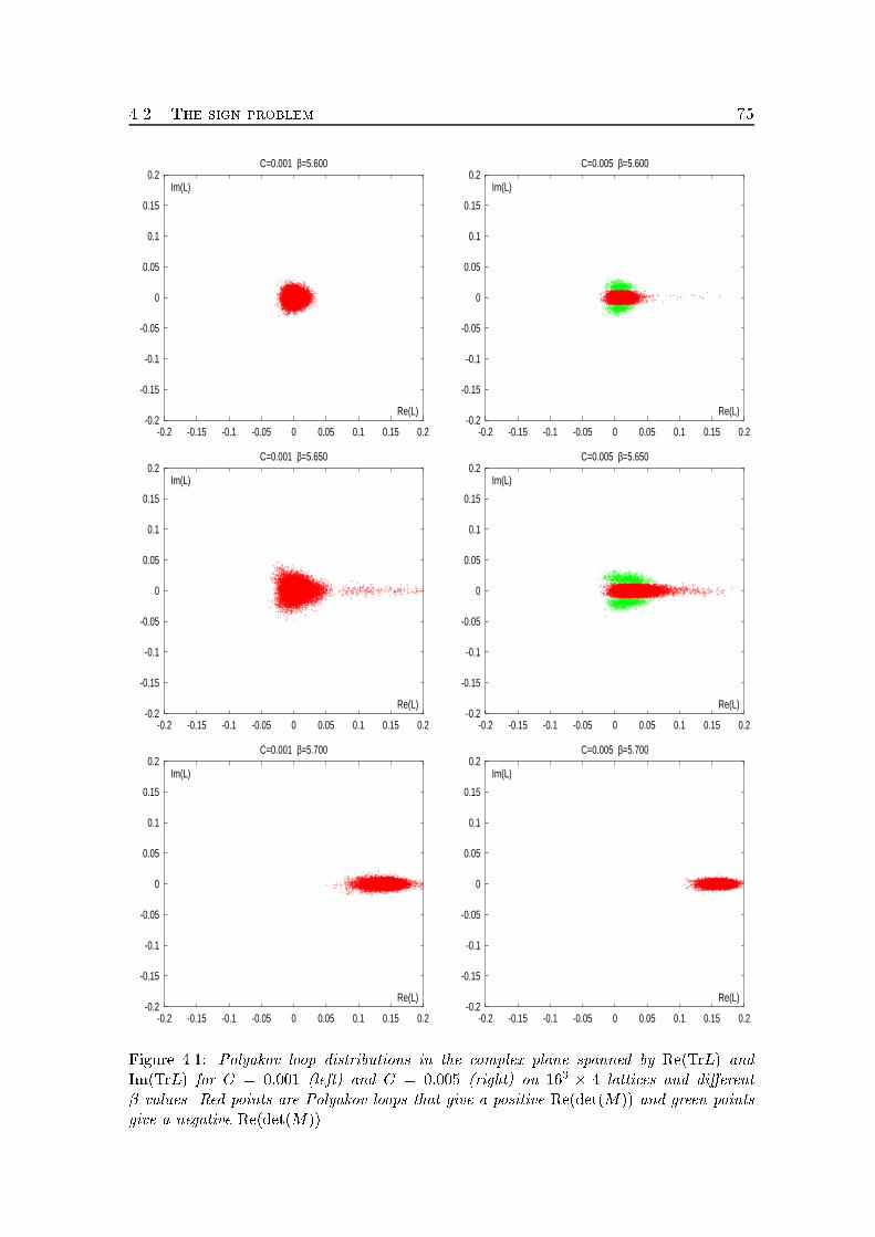
4.2. The sign problem 75

-0.2

-0.15

-0.1

-0.05

0

0.05

0.1

0.15

0.2

-0.2 -0.15 -0.1 -0.05 0 0.05 0.1 0.15 0.2

C=0.001 β=5.600

Re(L)

Im(L)

-0.2

-0.15

-0.1

-0.05

0

0.05

0.1

0.15

0.2

-0.2 -0.15 -0.1 -0.05 0 0.05 0.1 0.15 0.2

C=0.005 β=5.600

Re(L)

Im(L)

-0.2

-0.15

-0.1

-0.05

0

0.05

0.1

0.15

0.2

-0.2 -0.15 -0.1 -0.05 0 0.05 0.1 0.15 0.2

C=0.001 β=5.650

Re(L)

Im(L)

-0.2

-0.15

-0.1

-0.05

0

0.05

0.1

0.15

0.2

-0.2 -0.15 -0.1 -0.05 0 0.05 0.1 0.15 0.2

C=0.005 β=5.650

Re(L)

Im(L)

-0.2

-0.15

-0.1

-0.05

0

0.05

0.1

0.15

0.2

-0.2 -0.15 -0.1 -0.05 0 0.05 0.1 0.15 0.2

C=0.001 β=5.700

Re(L)

Im(L)

-0.2

-0.15

-0.1

-0.05

0

0.05

0.1

0.15

0.2

-0.2 -0.15 -0.1 -0.05 0 0.05 0.1 0.15 0.2

C=0.005 β=5.700

Re(L)

Im(L)

Figure 4.1: Polyakov loop distributions in the complex plane spanned by Re(TrL) andIm(TrL) for C = 0:001 (left) and C = 0:005 (right) on 163 � 4 lattices and di�erent�-values. Red points are Polyakov loops that give a positive Re(det(M)) and green pointsgive a negative Re(det(M)).

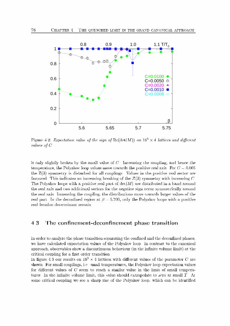
76 Chapter 4. The quenched limit in the grand canonical approach

0

0.2

0.4

0.6

0.8

1

5.6 5.65 5.7 5.75

0.8 0.9 1.0 1.1 T/Tc

β

C=0.0100C=0.0050C=0.0020C=0.0010C=0.0008

Figure 4.2: Expectation value of the sign of Re(det(M)) on 163 � 4 lattices and di�erentvalues of C.is only slightly broken by the small value of C. Increasing the coupling, and hence thetemperature, the Polyakov loop values move towards the positive real axis. For C = 0:005the Z(3) symmetry is disturbed for all couplings. Values in the positive real sector arefavoured. This indicates an increasing breaking of the Z(3) symmetry with increasing C.The Polyakov loops with a positive real part of det(M) are distributed in a band aroundthe real axis and two additional sectors for the negative sign occur symmetrically aroundthe real axis. Increasing the coupling, the distributions move towards larger values of thereal part. In the decon�ned region at � = 5:700, only the Polyakov loops with a positivereal fermion determinant remain.4.3 The con�nement-decon�nement phase transitionIn order to analyze the phase transition separating the con�ned and the decon�ned phases,we have calculated expectation values of the Polyakov loop. In contrast to the canonicalapproach, observables show a discontinuous behaviour (in the in�nite volume limit) at thecritical coupling for a �rst order transition.In �gure 4.3 our results on 163 � 4 lattices with di�erent values of the parameter C areshown. For small couplings, i.e. small temperatures, the Polyakov loop expectation valuesfor di�erent values of C seem to reach a similar value in the limit of small tempera-tures. In the in�nite volume limit, this value should extrapolate to zero at small T . Atsome critical coupling we see a sharp rise of the Polyakov loop, which can be identi�ed

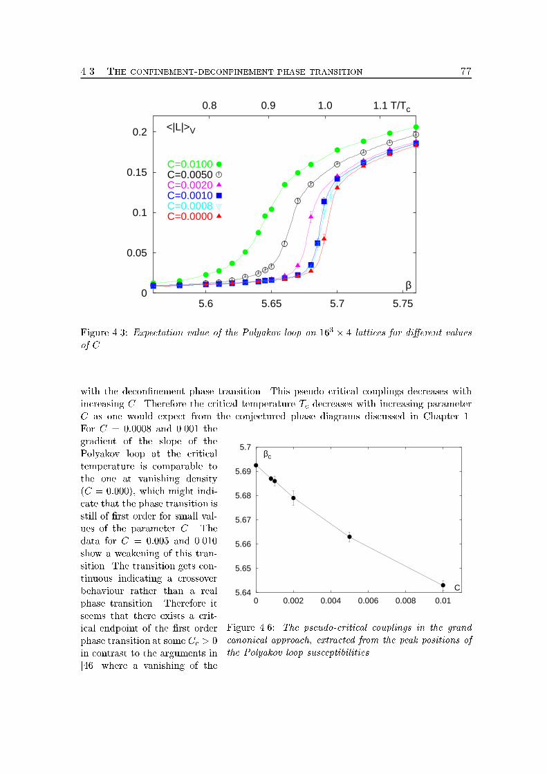
4.3. The confinement-deconfinement phase transition 77

0

0.05

0.1

0.15

0.2

5.6 5.65 5.7 5.75

0.8 0.9 1.0 1.1 T/Tc

β

<|L|>V

C=0.0100C=0.0050C=0.0020C=0.0010C=0.0008C=0.0000

Figure 4.3: Expectation value of the Polyakov loop on 163 � 4 lattices for di�erent valuesof C.with the decon�nement phase transition. This pseudo critical couplings decreases withincreasing C. Therefore the critical temperature Tc decreases with increasing parameterC as one would expect from the conjectured phase diagrams discussed in Chapter 1.

5.64

5.65

5.66

5.67

5.68

5.69

5.7

0 0.002 0.004 0.006 0.008 0.01

C

βc

Figure 4.6: The pseudo-critical couplings in the grandcanonical approach, extracted from the peak positions ofthe Polyakov loop susceptibilities.

For C = 0:0008 and 0.001 thegradient of the slope of thePolyakov loop at the criticaltemperature is comparable tothe one at vanishing density(C = 0:000), which might indi-cate that the phase transition isstill of �rst order for small val-ues of the parameter C. Thedata for C = 0:005 and 0.010show a weakening of this tran-sition. The transition gets con-tinuous indicating a crossoverbehaviour rather than a realphase transition. Therefore itseems that there exists a crit-ical endpoint of the �rst orderphase transition at some Cc > 0in contrast to the arguments in[46] where a vanishing of the

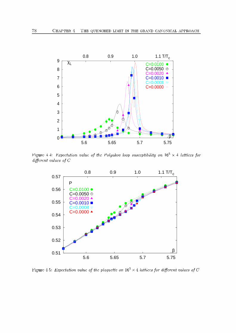
78 Chapter 4. The quenched limit in the grand canonical approach

0

1

2

3

4

5

6

7

8

9

5.6 5.65 5.7 5.75

0.8 0.9 1.0 1.1 T/Tc

β

χL C=0.0100C=0.0050C=0.0020C=0.0010C=0.0008C=0.0000

Figure 4.4: Expectation value of the Polyakov loop susceptibility on 163 � 4 lattices fordi�erent values of C.

0.51

0.52

0.53

0.54

0.55

0.56

0.57

5.6 5.65 5.7 5.75

0.8 0.9 1.0 1.1 T/Tc

β

PC=0.0100C=0.0050C=0.0020C=0.0010C=0.0008C=0.0000

Figure 4.5: Expectation value of the plaquette on 163� 4 lattices for di�erent values of C.

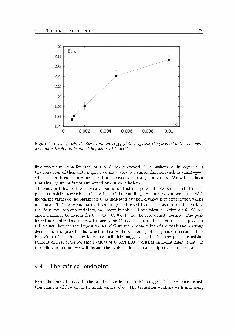
4.4. The critical endpoint 79

1.4

1.6

1.8

2

2.2

2.4

2.6

2.8

3

0 0.002 0.004 0.006 0.008 0.01

C

B4,M

Figure 4.7: The fourth Binder cumulant B4;M plotted against the parameter C. The solidline indicates the universal Ising value of 1.604(1).�rst order transition for any non-zero C was proposed. The authors of [46] argue thatthe behaviour of their data might be comparable to a simple function such as tanh(T�Tchx )which has a discontinuity for h ! 0 but a crossover at any non-zero h. We will see laterthat this argument is not supported by our calculations.The susceptibility of the Polyakov loop is plotted in �gure 4.4. We see the shift of thephase transition towards smaller values of the coupling, i.e. smaller temperatures, withincreasing values of the parameter C as indicated by the Polyakov loop expectation valuesin �gure 4.3. The pseudo-critical couplings, extracted from the position of the peak ofthe Polyakov loop susceptibility, are shown in table 4.4 and plotted in �gure 4.6. We seeagain a similar behaviour for C = 0:0008, 0.001 and the zero density results. The peakheight is slightly decreasing with increasing C but there is no broadening of the peak forthis values. For the two largest values of C we see a broadening of the peak and a strongdecrease of the peak height, which indicates the weakening of the phase transition. Thisbehaviour of the Polyakov loop susceptibilities suggests again that the phase transitionremains of �rst order for small values of C and that a critical endpoint might exist. Inthe following section we will discuss the evidence for such an endpoint in more detail.4.4 The critical endpointFrom the data discussed in the previous section, one might suggest that the phase transi-tion remains of �rst order for small values of C. The transition weakens with increasing

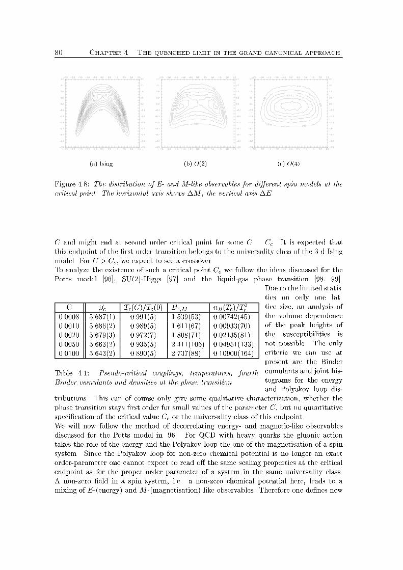
80 Chapter 4. The quenched limit in the grand canonical approach

(a) Ising (b) O(2) (c) O(4)Figure 4.8: The distribution of E- and M-like observables for di�erent spin models at thecritical point. The horizontal axis shows �M , the vertical axis �E.C and might end at second order critical point for some C = Cc. It is expected thatthis endpoint of the �rst order transition belongs to the universality class of the 3-d Isingmodel. For C > Cc, we expect to see a crossover.To analyze the existence of such a critical point Cc we follow the ideas discussed for thePotts model [96], SU(2)-Higgs [97] and the liquid-gas phase transition [98, 99].C �c Tc(C)=Tc(0) B4;M nB(Tc)=T 3c0.0008 5.687(1) 0.991(5) 1.539(53) 0.00742(45)0.0010 5.686(2) 0.989(5) 1.611(67) 0.00933(70)0.0020 5.679(3) 0.972(7) 1.808(71) 0.02135(81)0.0050 5.663(2) 0.935(5) 2.411(106) 0.04951(133)0.0100 5.643(2) 0.890(5) 2.737(88) 0.10900(164)Table 4.1: Pseudo-critical couplings, temperatures, fourthBinder cumulants and densities at the phase transition.

Due to the limited statis-tics on only one lat-tice size, an analysis ofthe volume dependenceof the peak heights ofthe susceptibilities isnot possible. The onlycriteria we can use atpresent are the Bindercumulants and joint his-tograms for the energyand Polyakov loop dis-tributions. This can of course only give some qualitative characterization, whether thephase transition stays �rst order for small values of the parameter C, but no quantitativespeci�cation of the critical value Cc or the universality class of this endpoint.We will now follow the method of decorrelating energy- and magnetic-like observablesdiscussed for the Potts model in [96]. For QCD with heavy quarks the gluonic actiontakes the role of the energy and the Polyakov loop the one of the magnetisation of a spinsystem. Since the Polyakov loop for non-zero chemical potential is no longer an exactorder-parameter one cannot expect to read o� the same scaling properties at the criticalendpoint as for the proper order parameter of a system in the same universality class.A non-zero �eld in a spin system, i.e. a non-zero chemical potential here, leads to amixing of E-(energy) and M -(magnetisation) like observables. Therefore one de�nes new

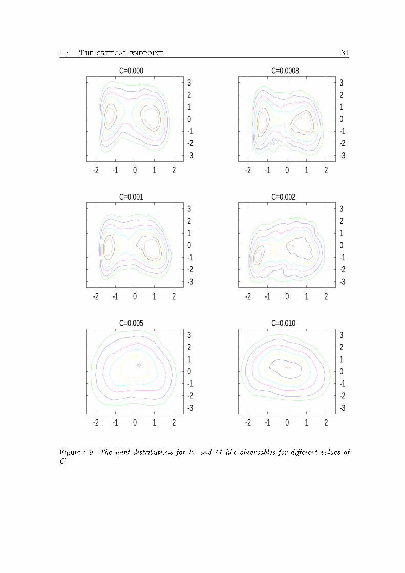
4.4. The critical endpoint 81C=0.000

-2 -1 0 1 2

-3-2-10123

C=0.0008

-2 -1 0 1 2

-3-2-10123

C=0.001

-2 -1 0 1 2

-3-2-10123

C=0.002

-2 -1 0 1 2

-3-2-10123

C=0.005

-2 -1 0 1 2

-3-2-10123

C=0.010

-2 -1 0 1 2

-3-2-10123

Figure 4.9: The joint distributions for E- and M -like observables for di�erent values ofC.

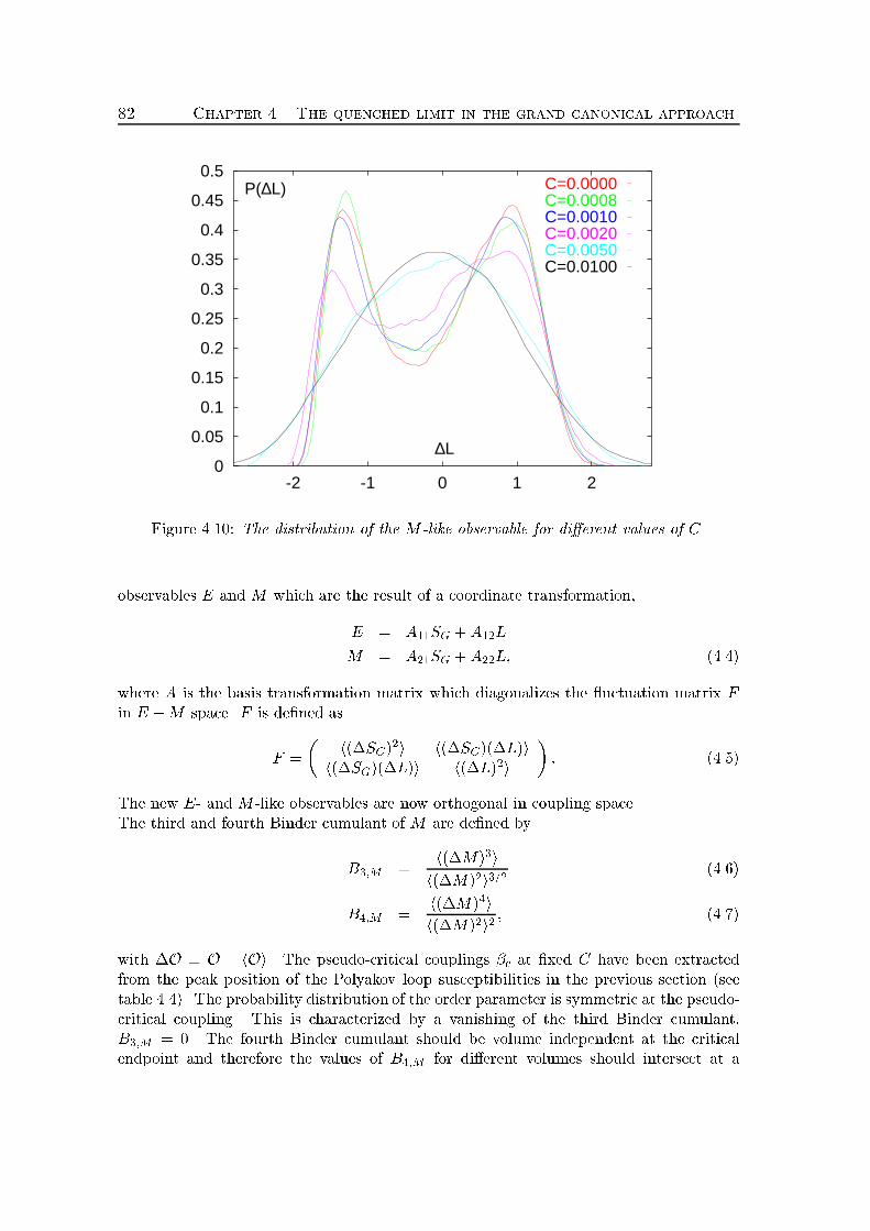
82 Chapter 4. The quenched limit in the grand canonical approach

0

0.05

0.1

0.15

0.2

0.25

0.3

0.35

0.4

0.45

0.5

-2 -1 0 1 2

∆L

P(∆L) C=0.0000C=0.0008C=0.0010C=0.0020C=0.0050C=0.0100

Figure 4.10: The distribution of the M -like observable for di�erent values of C.observables E and M which are the result of a coordinate transformation,E = A11SG +A12LM = A21SG +A22L; (4.4)where A is the basis transformation matrix which diagonalizes the uctuation matrix Fin E �M space. F is de�ned asF = � h(�SG)2i h(�SG)(�L)ih(�SG)(�L)i h(�L)2i � : (4.5)The new E- and M -like observables are now orthogonal in coupling space.The third and fourth Binder cumulant of M are de�ned byB3;M = h(�M)3ih(�M)2i3=2 (4.6)B4;M = h(�M)4ih(�M)2i2 ; (4.7)with �O � O � hOi. The pseudo-critical couplings �c at �xed C have been extractedfrom the peak position of the Polyakov loop susceptibilities in the previous section (seetable 4.4). The probability distribution of the order parameter is symmetric at the pseudo-critical coupling. This is characterized by a vanishing of the third Binder cumulant,B3;M = 0. The fourth Binder cumulant should be volume independent at the criticalendpoint and therefore the values of B4;M for di�erent volumes should intersect at a

4.5. The baryon number density 83universal value Cc. In [96] it was shown that for the Potts model, the critical external �eldis in very good agreement with the universal Ising value of 1.604(1). The universal valuesfor O(2) and O(4) are 1.092(3) and 1.233(6). The results for the fourth Binder cumulantare shown in table 4.4. In �gure 4.7 we see that the fourth Binder cumulant reaches theuniversal Ising value for a value of the parameter C around 0.001. This value might serveas a �rst indication for the critical point. Simulations on larger lattices are needed to seeif the Binder cumulants intersect at this point.The distribution of the M -like observable is plotted in �gure 4.10. We see a clear double-peak structure up to C = 0:001, indicating the existence of a phase transition. For thelarge values of C, only one symmetric peak remains showing a crossover behaviour. Thisbehaviour favors again a value of Cc around 0.001.Finally we analyze the joint E- and M -like distributions. They are normalized suchthat h(�M)2i = 1 and h(�E)2i = 1. For the di�erent universality classes discussed inconnection with the Potts model and QCD, the Ising, O(4) and O(2) joint distributionsat the critical endpoint are plotted in �gure 4.8. The joint distributions of the rotatedPolyakov loop M and the rotated action E are investigated on 163 � 4 lattices at thepseudo critical coupling. They are plotted in �gure 4.9 for di�erent values of C. Thedistributions for C = 0:000 and 0.0008 look quite similar indicating the �rst order natureof the transition. For C = 0:001 one �nds a certain structure in the distribution whichshows feature of the Ising or O(2) distribution shown in �gure 4.8. The distribution forC > 0:002 look more like a crossover. The two largest values show a rotationally symmetricdistribution which is a clear signal for a crossover. Therefore one might conclude thatthe transition is still of �rst order for small values of C and turns into a crossover atapproximately C � 0:001 � 0:002. However, for the joint distributions the lattice volumeand the statistics seems to be too small to determine an exact position of the criticalendpoint. Simulations on larger lattices are needed to determine the location of the criticalpoint and its universality class. We have seen that the methods used for the Potts modelalso seem to work for QCD at non-zero chemical potential.4.5 The baryon number densityUnlike in the canonical approach, the baryon number density is an observable in the grandcanonical approach. It can be calculated by the derivative of the logarithm of the partitionfunction with respect to the chemical potential �,hnBiT 3 = 13T 3 1aN�V @ln(Z)@� (4.8)= 2N3�3N3� *X~x C2TrP~x + 2CTrP y~x + 3C3 +C2TrP~x +CTrP y~x + 1+ (4.9)The results for nB=T 3 are shown in �gure 4.11 and �gure 4.12. Below the critical temper-ature the density is small. It shows a strong increase at the phase transition and turns tolarge values in the decon�ned phase. With increasing value of the parameter C, the baryonnumber density rises towards larger values. For the smallest values of C the slope of the

84 Chapter 4. The quenched limit in the grand canonical approachdensity at the critical coupling is very steep comparable to the behaviour of the Polyakovloop expectation values in �gure 4.3. This indicates again that the phase transition is of�rst order for small values of C. The densities at the pseudo-critical couplings are shownin table 4.4.All baryon number densities which we have analyzed in the canonical approach seem to bein the crossover region, rather than in the region of �rst order phase transition. Thereforeit is not surprising that we have found no clear signals for a region of coexisting phases inthe canonical approach. The broadening of the phase transition region might also be ex-plained by a cross-over behaviour. Simulations for even smaller densities in the canonicalapproach have to be performed to see signals for a region of coexisting phases.

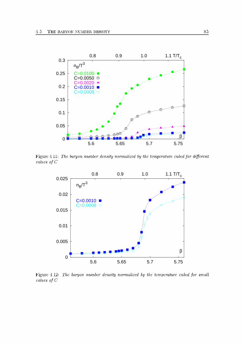
4.5. The baryon number density 85

0

0.05

0.1

0.15

0.2

0.25

0.3

5.6 5.65 5.7 5.75

0.8 0.9 1.0 1.1 T/Tc

β

nB/T3

C=0.0100C=0.0050C=0.0020C=0.0010C=0.0008

Figure 4.11: The baryon number density normalized by the temperature cubed for di�erentvalues of C.

0

0.005

0.01

0.015

0.02

0.025

5.6 5.65 5.7 5.75

0.8 0.9 1.0 1.1 T/Tc

β

nB/T3

C=0.0010C=0.0008

Figure 4.12: The baryon number density normalized by the temperature cubed for smallvalues of C.

86

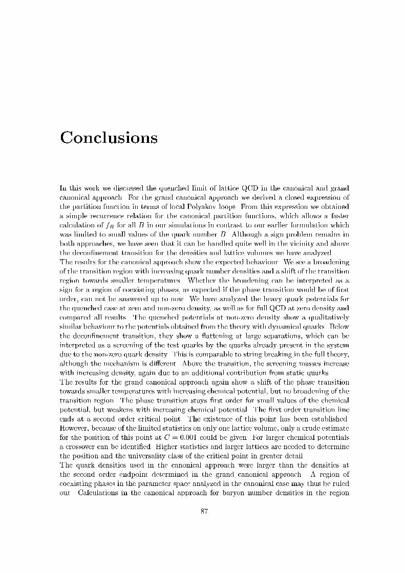
ConclusionsIn this work we discussed the quenched limit of lattice QCD in the canonical and grandcanonical approach. For the grand canonical approach we derived a closed expression ofthe partition function in terms of local Polyakov loops. From this expression we obtaineda simple recurrence relation for the canonical partition functions, which allows a fastercalculation of fB for all B in our simulations in contrast to our earlier formulation whichwas limited to small values of the quark number B. Although a sign problem remains inboth approaches, we have seen that it can be handled quite well in the vicinity and abovethe decon�nement transition for the densities and lattice volumes we have analyzed.The results for the canonical approach show the expected behaviour. We see a broadeningof the transition region with increasing quark number densities and a shift of the transitionregion towards smaller temperatures. Whether the broadening can be interpreted as asign for a region of coexisting phases, as expected if the phase transition would be of �rstorder, can not be answered up to now. We have analyzed the heavy quark potentials forthe quenched case at zero and non-zero density, as well as for full QCD at zero density andcompared all results. The quenched potentials at non-zero density show a qualitativelysimilar behaviour to the potentials obtained from the theory with dynamical quarks. Belowthe decon�nement transition, they show a attening at large separations, which can beinterpreted as a screening of the test quarks by the quarks already present in the systemdue to the non-zero quark density. This is comparable to string breaking in the full theory,although the mechanism is di�erent. Above the transition, the screening masses increasewith increasing density, again due to an additional contribution from static quarks.The results for the grand canonical approach again show a shift of the phase transitiontowards smaller temperatures with increasing chemical potential, but no broadening of thetransition region. The phase transition stays �rst order for small values of the chemicalpotential, but weakens with increasing chemical potential. The �rst order transition lineends at a second order critical point. The existence of this point has been established.However, because of the limited statistics on only one lattice volume, only a crude estimatefor the position of this point at C = 0:001 could be given. For larger chemical potentialsa crossover can be identi�ed. Higher statistics and larger lattices are needed to determinethe position and the universality class of the critical point in greater detail.The quark densities used in the canonical approach were larger than the densities atthe second order endpoint determined in the grand canonical approach. A region ofcoexisting phases in the parameter space analyzed in the canonical case may thus be ruledout. Calculations in the canonical approach for baryon number densities in the region87

88of the �rst order transition, i.e. at even smaller densities, are needed to observe signalsfor a region of coexisting phases. Larger lattices might improve the signatures for thiscoexistence, but will also lead to a more severe sign problem. Therefore the formulationand algorithms have to be improved to handle, or even remove, the sign problem also forlarger lattice volumes.With this work we intended to explore a new starting point for a non-perturbative analysisof QCD at �nite density on the lattice. Within the static approximation we could establishmany of the basic changes in the thermodynamic behaviour of QCD that are expectedto occur in the presence of a non-vanishing baryon number density. The screening ofthe heavy quark potential and the reduction of chiral symmetry breaking are the moststriking e�ects. The next step will be to allow for large, but �nite quark masses, whichwill include also the propagation of the quarks in spatial direction. As the sign problemwill be enhanced in this case, new algorithms or di�erent formulations of the theory needto be developed. Further e�ort in this �eld will hopefully lead to a better understandingof the physics of strongly interacting matter as it will be created in experiments, existedin the early universe and might exist in the cores of compact stars.

Appendix ATables of the results

89

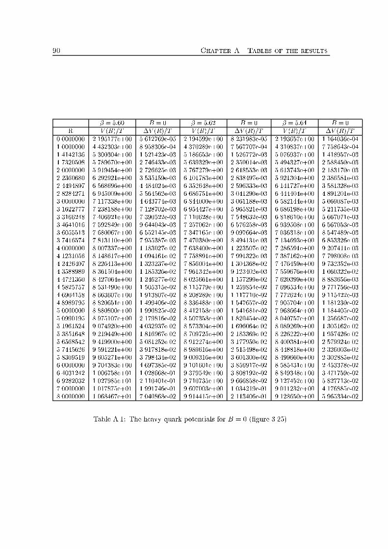
90 Chapter A. Tables of the results� = 5:60 B = 0 � = 5:62 B = 0 � = 5:64 B = 0R V (R)=T �V (R)=T V (R)=T �V (R)=T V (R)=T �V (R)=T0.0000000 2.195177e+00 5.612769e-05 2.194599e+00 8.231983e-05 2.193657e+00 1.164036e-041.0000000 4.432303e+00 8.958306e-04 4.370289e+00 7.567707e-04 4.310837e+00 7.758643e-041.4142136 5.300304e+00 1.521423e-03 5.186653e+00 1.526772e-03 5.076937e+00 1.418957e-031.7320508 5.789670e+00 2.746433e-03 5.639329e+00 2.350014e-03 5.494327e+00 2.588450e-032.0000000 5.919454e+00 2.726625e-03 5.767279e+00 2.618553e-03 5.613743e+00 2.183170e-032.2360680 6.292921e+00 3.535159e-03 6.101783e+00 2.838497e-03 5.921304e+00 2.386581e-032.4494897 6.568696e+00 4.484024e-03 6.352648e+00 2.596333e-03 6.141727e+00 3.581328e-032.8284271 6.945009e+00 5.564562e-03 6.686751e+00 3.041290e-03 6.444404e+00 4.891201e-033.0000000 7.117338e+00 4.643774e-03 6.844000e+00 3.061188e-03 6.582144e+00 5.069087e-033.1622777 7.238188e+00 7.128702e-03 6.954427e+00 5.965821e-03 6.686198e+00 5.211735e-033.3166248 7.406921e+00 7.390522e-03 7.110628e+00 7.548632e-03 6.818610e+00 5.667071e-033.4641016 7.592849e+00 9.644043e-03 7.257062e+00 6.576258e-03 6.939508e+00 6.567053e-033.6055513 7.680067e+00 6.552145e-03 7.347165e+00 9.097664e-03 7.036318e+00 8.547489e-033.7416574 7.813110e+00 7.955387e-03 7.470380e+00 8.494131e-03 7.134693e+00 6.853326e-034.0000000 8.007337e+00 1.183027e-02 7.638400e+00 1.223507e-02 7.286591e+00 9.207411e-034.1231056 8.148617e+00 1.094161e-02 7.758891e+00 7.991322e-03 7.387162e+00 7.798008e-034.2426407 8.226413e+00 1.323237e-02 7.856004e+00 1.304368e-02 7.476459e+00 9.732352e-034.3588989 8.361504e+00 1.185326e-02 7.961342e+00 9.123402e-03 7.559676e+00 1.060322e-024.4721360 8.427064e+00 1.246277e-02 8.025661e+00 1.157299e-02 7.620399e+00 8.883656e-034.5825757 8.531490e+00 1.505315e-02 8.115779e+00 1.259854e-02 7.696534e+00 9.771756e-034.6904158 8.663607e+00 1.913807e-02 8.208289e+00 1.117710e-02 7.772624e+00 9.115422e-034.8989795 8.820651e+00 1.499406e-02 8.336488e+00 1.547657e-02 7.905704e+00 1.181230e-025.0000000 8.880800e+00 1.990825e-02 8.412158e+00 1.541681e-02 7.968664e+00 1.184405e-025.0990195 8.975107e+00 2.179816e-02 8.507358e+00 1.820454e-02 8.040757e+00 1.256687e-025.1961524 9.074920e+00 4.032937e-02 8.573304e+00 1.696064e-02 8.089269e+00 1.305162e-025.3851648 9.219449e+00 1.816967e-02 8.709725e+00 2.183369e-02 8.226222e+00 1.957426e-025.6568542 9.419900e+00 5.081252e-02 8.912274e+00 3.177950e-02 8.400381e+00 2.579924e-025.7445626 9.591221e+00 3.917818e-02 8.989616e+00 2.515498e-02 8.448818e+00 2.326003e-025.8309519 9.605271e+00 3.798434e-02 9.009316e+00 3.601300e-02 8.499660e+00 2.302885e-026.0000000 9.704383e+00 4.697385e-02 9.101601e+00 3.856917e-02 8.585431e+00 2.453378e-026.4031242 1.006758e+01 1.028668e-01 9.379549e+00 3.808192e-02 8.849348e+00 3.471759e-026.9282032 1.027985e+01 2.110401e-01 9.710735e+00 9.666858e-02 9.127452e+00 5.827713e-027.0000000 1.017875e+01 1.991746e-01 9.607003e+00 1.034219e-01 9.011232e+00 4.176885e-028.0000000 1.068467e+01 7.040868e-02 9.914415e+00 2.113406e-01 9.128650e+00 5.965334e-02Table A.1: The heavy quark potentials for B = 0 (�gure 3.25).

91� = 5:66 B = 0 � = 5:68 B = 0 � = 5:60 B = 6R V (R)=T �V (R)=T V (R)=T �V (R)=T V (R)=T �V (R)=T0.0000 2.192093e+00 1.463824e-04 2.187407e+00 2.124049e-04 2.189309e+00 1.848690e-031.0000 4.248518e+00 1.313626e-03 4.159960e+00 1.908997e-03 4.341691e+00 1.191301e-021.4142 4.965017e+00 2.398089e-03 4.799412e+00 4.062993e-03 5.085961e+00 2.365677e-021.7320 5.343720e+00 3.756978e-03 5.120896e+00 5.732179e-03 5.436481e+00 4.024753e-022.0000 5.453846e+00 3.946189e-03 5.210577e+00 6.133714e-03 5.569226e+00 3.865565e-022.2360 5.725858e+00 4.670958e-03 5.428492e+00 7.793819e-03 5.821445e+00 4.749981e-022.4494 5.922896e+00 6.135797e-03 5.581695e+00 8.995278e-03 6.014012e+00 5.072183e-022.8284 6.189226e+00 7.798261e-03 5.780578e+00 1.161951e-02 6.188327e+00 6.303483e-023.0000 6.308142e+00 8.439360e-03 5.866399e+00 1.272150e-02 6.272407e+00 6.222171e-023.1622 6.399997e+00 8.105853e-03 5.931206e+00 1.364072e-02 6.329784e+00 7.812033e-023.3166 6.512949e+00 8.722369e-03 6.009849e+00 1.460781e-02 6.437798e+00 8.405653e-023.4641 6.627455e+00 1.093301e-02 6.084376e+00 1.555820e-02 6.475336e+00 1.011344e-013.6055 6.700295e+00 1.181394e-02 6.133100e+00 1.647286e-02 6.475413e+00 8.625004e-023.7416 6.788959e+00 1.180710e-02 6.192047e+00 1.752462e-02 6.563706e+00 6.547030e-024.0000 6.918046e+00 1.575112e-02 6.275205e+00 1.917228e-02 6.625047e+00 9.693986e-024.1231 7.005587e+00 1.515043e-02 6.328514e+00 2.006806e-02 6.672881e+00 9.359741e-024.2426 7.070548e+00 1.625915e-02 6.369246e+00 2.103500e-02 6.680095e+00 9.923598e-024.3588 7.152382e+00 1.653766e-02 6.413702e+00 2.189586e-02 6.722414e+00 8.805614e-024.4721 7.197069e+00 1.636643e-02 6.444787e+00 2.263997e-02 6.719153e+00 7.923854e-024.5825 7.260390e+00 1.976964e-02 6.481869e+00 2.325266e-02 6.749377e+00 9.267044e-024.6904 7.340721e+00 2.057044e-02 6.521900e+00 2.499226e-02 6.819791e+00 9.851563e-024.8989 7.437307e+00 2.128655e-02 6.579160e+00 2.574756e-02 6.816396e+00 7.130386e-025.0000 7.482835e+00 2.178571e-02 6.601542e+00 2.722543e-02 6.851878e+00 1.157425e-015.0990 7.536245e+00 2.521042e-02 6.633521e+00 2.806136e-02 6.842898e+00 8.663726e-025.1961 7.601146e+00 2.340587e-02 6.662079e+00 2.922988e-02 6.981169e+00 1.110530e-015.3851 7.697214e+00 2.781506e-02 6.710516e+00 2.957194e-02 6.837637e+00 9.290371e-025.6568 7.808134e+00 3.350697e-02 6.771349e+00 3.292517e-02 6.942538e+00 1.305804e-015.7445 7.860449e+00 2.842957e-02 6.793319e+00 3.222945e-02 6.892614e+00 1.049684e-015.8309 7.928702e+00 3.087645e-02 6.818589e+00 3.375375e-02 6.907084e+00 1.052762e-016.0000 7.977161e+00 3.124491e-02 6.848148e+00 3.398539e-02 6.924625e+00 1.227445e-016.4031 8.190880e+00 3.614668e-02 6.938800e+00 3.684048e-02 6.846521e+00 1.144498e-016.9282 8.412977e+00 4.748189e-02 7.029597e+00 4.065465e-02 6.949595e+00 1.513076e-017.0000 8.242425e+00 2.831035e-02 6.943296e+00 3.917749e-02 6.942942e+00 1.330674e-018.0000 8.351243e+00 5.898439e-02 6.982273e+00 3.974387e-02 7.035027e+00 1.488300e-01Table A.2: The heavy quark potentials for B = 0 (�gure 3.25) and for B = 6 (�gure 3.26).

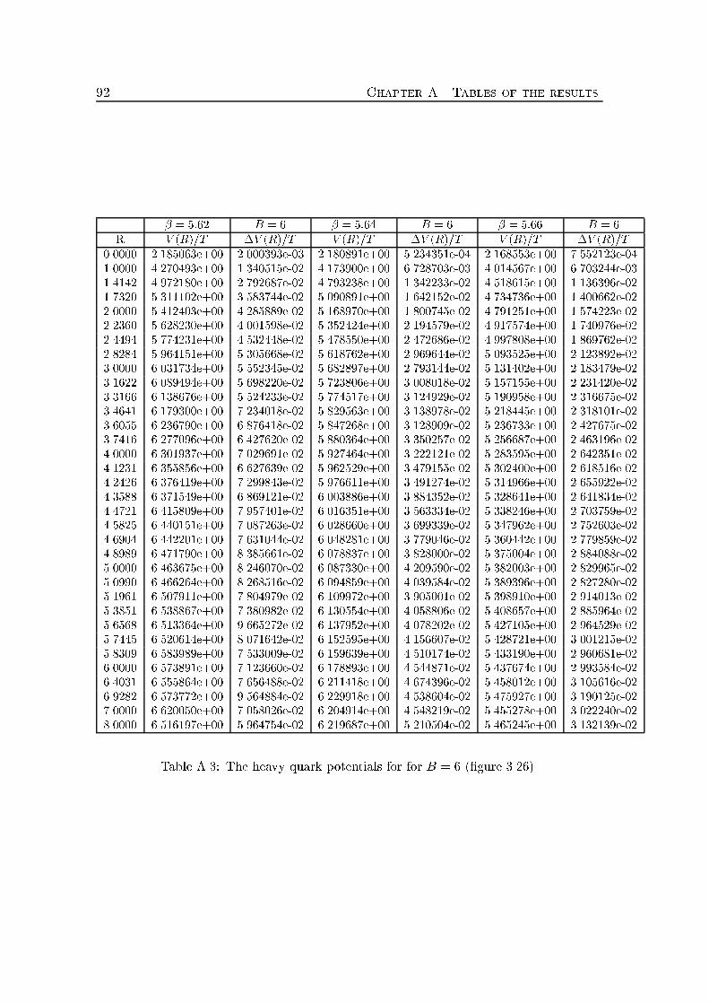
92 Chapter A. Tables of the results� = 5:62 B = 6 � = 5:64 B = 6 � = 5:66 B = 6R V (R)=T �V (R)=T V (R)=T �V (R)=T V (R)=T �V (R)=T0.0000 2.185063e+00 2.000393e-03 2.180891e+00 5.234351e-04 2.168553e+00 7.552123e-041.0000 4.270493e+00 1.340515e-02 4.173900e+00 6.728703e-03 4.014567e+00 6.703244e-031.4142 4.972180e+00 2.792687e-02 4.793238e+00 1.342233e-02 4.518615e+00 1.136396e-021.7320 5.311102e+00 3.583744e-02 5.090891e+00 1.642152e-02 4.734736e+00 1.400662e-022.0000 5.412403e+00 4.285889e-02 5.168970e+00 1.800745e-02 4.791251e+00 1.574223e-022.2360 5.628230e+00 4.001598e-02 5.352424e+00 2.194579e-02 4.917574e+00 1.740976e-022.4494 5.774231e+00 4.532448e-02 5.478550e+00 2.472686e-02 4.997808e+00 1.869762e-022.8284 5.964151e+00 5.305668e-02 5.618762e+00 2.969644e-02 5.093525e+00 2.123892e-023.0000 6.031734e+00 5.552345e-02 5.682897e+00 2.793144e-02 5.131402e+00 2.183479e-023.1622 6.089494e+00 5.698220e-02 5.723806e+00 3.008018e-02 5.157155e+00 2.231420e-023.3166 6.138676e+00 5.524233e-02 5.774517e+00 3.124929e-02 5.190958e+00 2.316675e-023.4641 6.179300e+00 7.234018e-02 5.829563e+00 3.138978e-02 5.218445e+00 2.318101e-023.6055 6.236790e+00 6.876418e-02 5.847268e+00 3.128909e-02 5.236733e+00 2.427675e-023.7416 6.277096e+00 6.427620e-02 5.880364e+00 3.350257e-02 5.256687e+00 2.463196e-024.0000 6.301937e+00 7.029691e-02 5.927464e+00 3.222121e-02 5.283595e+00 2.642351e-024.1231 6.355856e+00 6.627639e-02 5.962529e+00 3.479155e-02 5.302400e+00 2.618516e-024.2426 6.376419e+00 7.299843e-02 5.976611e+00 3.491274e-02 5.314966e+00 2.655922e-024.3588 6.371549e+00 6.869121e-02 6.003886e+00 3.884352e-02 5.328641e+00 2.641834e-024.4721 6.415809e+00 7.957401e-02 6.016351e+00 3.563334e-02 5.338246e+00 2.703759e-024.5825 6.440151e+00 7.087263e-02 6.028660e+00 3.699339e-02 5.347962e+00 2.752603e-024.6904 6.442201e+00 7.631044e-02 6.048281e+00 3.779046e-02 5.360442e+00 2.779859e-024.8989 6.471790e+00 8.385661e-02 6.078837e+00 3.828000e-02 5.375004e+00 2.884088e-025.0000 6.463675e+00 8.246070e-02 6.087330e+00 4.209590e-02 5.382003e+00 2.829965e-025.0990 6.466264e+00 8.268516e-02 6.094859e+00 4.039584e-02 5.389396e+00 2.827280e-025.1961 6.507911e+00 7.804979e-02 6.109972e+00 3.905001e-02 5.398910e+00 2.914013e-025.3851 6.538867e+00 7.380982e-02 6.130554e+00 4.058806e-02 5.408657e+00 2.885964e-025.6568 6.513364e+00 9.665272e-02 6.137952e+00 4.078202e-02 5.427105e+00 2.964529e-025.7445 6.520614e+00 8.071642e-02 6.152595e+00 4.156607e-02 5.428721e+00 3.001215e-025.8309 6.583989e+00 7.533009e-02 6.159639e+00 4.510174e-02 5.433190e+00 2.960681e-026.0000 6.573891e+00 7.123660e-02 6.178893e+00 4.544871e-02 5.437674e+00 2.993584e-026.4031 6.555864e+00 7.656488e-02 6.211418e+00 4.674396e-02 5.458012e+00 3.105616e-026.9282 6.573772e+00 9.564884e-02 6.229918e+00 4.538604e-02 5.475927e+00 3.190125e-027.0000 6.620050e+00 7.058026e-02 6.204914e+00 4.548219e-02 5.455278e+00 3.022240e-028.0000 6.516197e+00 5.964754e-02 6.219687e+00 5.210504e-02 5.465245e+00 3.132139e-02Table A.3: The heavy quark potentials for for B = 6 (�gure 3.26).

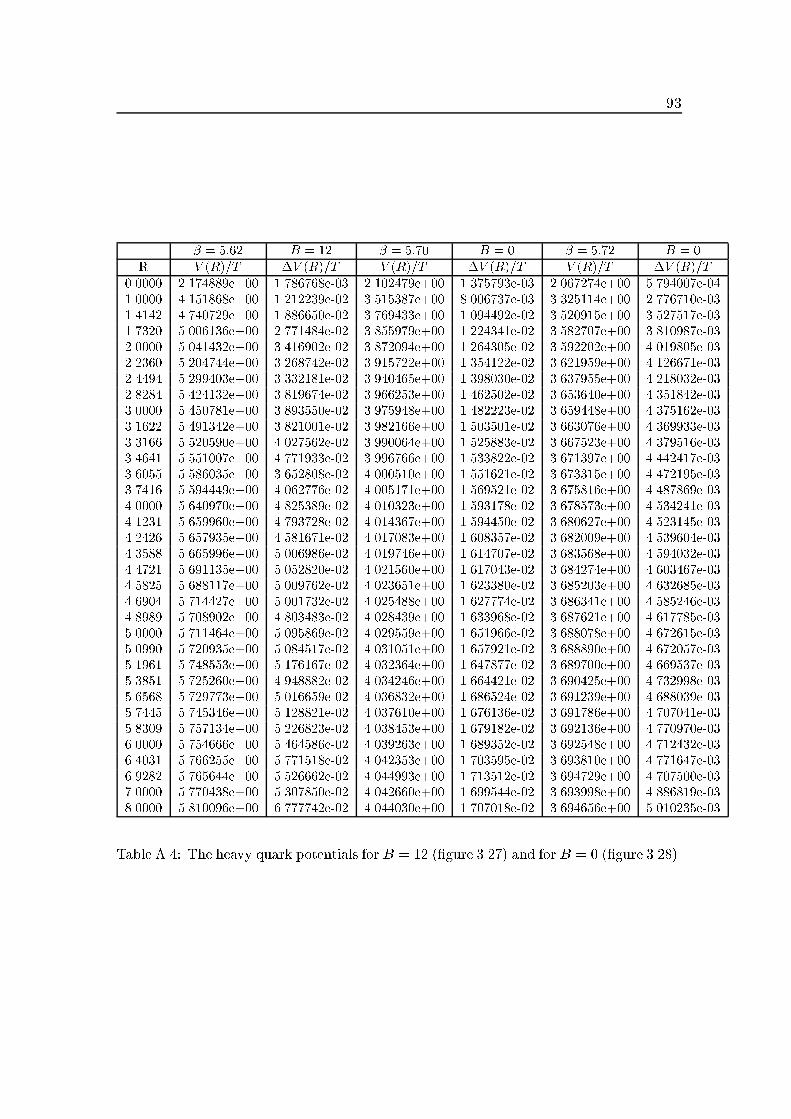
93� = 5:62 B = 12 � = 5:70 B = 0 � = 5:72 B = 0R V (R)=T �V (R)=T V (R)=T �V (R)=T V (R)=T �V (R)=T0.0000 2.174889e+00 1.786768e-03 2.102479e+00 1.375793e-03 2.067274e+00 5.794007e-041.0000 4.151868e+00 1.212239e-02 3.515387e+00 8.006737e-03 3.325114e+00 2.776710e-031.4142 4.740729e+00 1.886650e-02 3.769433e+00 1.094492e-02 3.520915e+00 3.527517e-031.7320 5.006136e+00 2.771484e-02 3.855979e+00 1.224341e-02 3.582707e+00 3.810987e-032.0000 5.041432e+00 3.416902e-02 3.872094e+00 1.264305e-02 3.592202e+00 4.019805e-032.2360 5.204744e+00 3.268742e-02 3.915722e+00 1.354122e-02 3.621959e+00 4.126671e-032.4494 5.299403e+00 3.332181e-02 3.940465e+00 1.398030e-02 3.637955e+00 4.218032e-032.8284 5.424132e+00 3.819674e-02 3.966253e+00 1.462502e-02 3.653640e+00 4.351842e-033.0000 5.450781e+00 3.893550e-02 3.975948e+00 1.482223e-02 3.659448e+00 4.375162e-033.1622 5.491342e+00 3.821001e-02 3.982166e+00 1.503501e-02 3.663076e+00 4.369933e-033.3166 5.520590e+00 4.027562e-02 3.990064e+00 1.525883e-02 3.667523e+00 4.379516e-033.4641 5.551007e+00 4.771933e-02 3.996766e+00 1.533822e-02 3.671397e+00 4.442417e-033.6055 5.586035e+00 3.652808e-02 4.000510e+00 1.551621e-02 3.673315e+00 4.472195e-033.7416 5.594449e+00 4.062776e-02 4.005171e+00 1.569521e-02 3.675816e+00 4.487869e-034.0000 5.640970e+00 4.825389e-02 4.010323e+00 1.593178e-02 3.678573e+00 4.534241e-034.1231 5.659960e+00 4.793728e-02 4.014367e+00 1.594450e-02 3.680627e+00 4.523145e-034.2426 5.657935e+00 4.581671e-02 4.017083e+00 1.608357e-02 3.682009e+00 4.539604e-034.3588 5.665996e+00 5.006986e-02 4.019746e+00 1.614707e-02 3.683568e+00 4.594032e-034.4721 5.691135e+00 5.052820e-02 4.021560e+00 1.617043e-02 3.684274e+00 4.603467e-034.5825 5.688117e+00 5.009762e-02 4.023651e+00 1.623380e-02 3.685203e+00 4.632685e-034.6904 5.714427e+00 5.001732e-02 4.025488e+00 1.627774e-02 3.686341e+00 4.585246e-034.8989 5.708902e+00 4.803483e-02 4.028439e+00 1.633968e-02 3.687621e+00 4.617785e-035.0000 5.711464e+00 5.095869e-02 4.029559e+00 1.651966e-02 3.688078e+00 4.672615e-035.0990 5.720935e+00 5.084517e-02 4.031051e+00 1.657921e-02 3.688890e+00 4.672057e-035.1961 5.748553e+00 5.176167e-02 4.032364e+00 1.647877e-02 3.689700e+00 4.669537e-035.3851 5.725260e+00 4.948882e-02 4.034246e+00 1.664421e-02 3.690425e+00 4.732998e-035.6568 5.729773e+00 5.016659e-02 4.036832e+00 1.686524e-02 3.691239e+00 4.688039e-035.7445 5.745346e+00 5.128821e-02 4.037610e+00 1.676136e-02 3.691786e+00 4.707041e-035.8309 5.757134e+00 5.226823e-02 4.038453e+00 1.679182e-02 3.692136e+00 4.770970e-036.0000 5.754666e+00 5.464586e-02 4.039263e+00 1.689352e-02 3.692548e+00 4.712432e-036.4031 5.766255e+00 5.771518e-02 4.042353e+00 1.703595e-02 3.693810e+00 4.771647e-036.9282 5.765644e+00 5.526662e-02 4.044993e+00 1.713512e-02 3.694729e+00 4.707500e-037.0000 5.770438e+00 5.307850e-02 4.042660e+00 1.699544e-02 3.693998e+00 4.886819e-038.0000 5.810096e+00 6.777742e-02 4.044030e+00 1.707018e-02 3.694656e+00 5.010235e-03Table A.4: The heavy quark potentials for B = 12 (�gure 3.27) and for B = 0 (�gure 3.28).

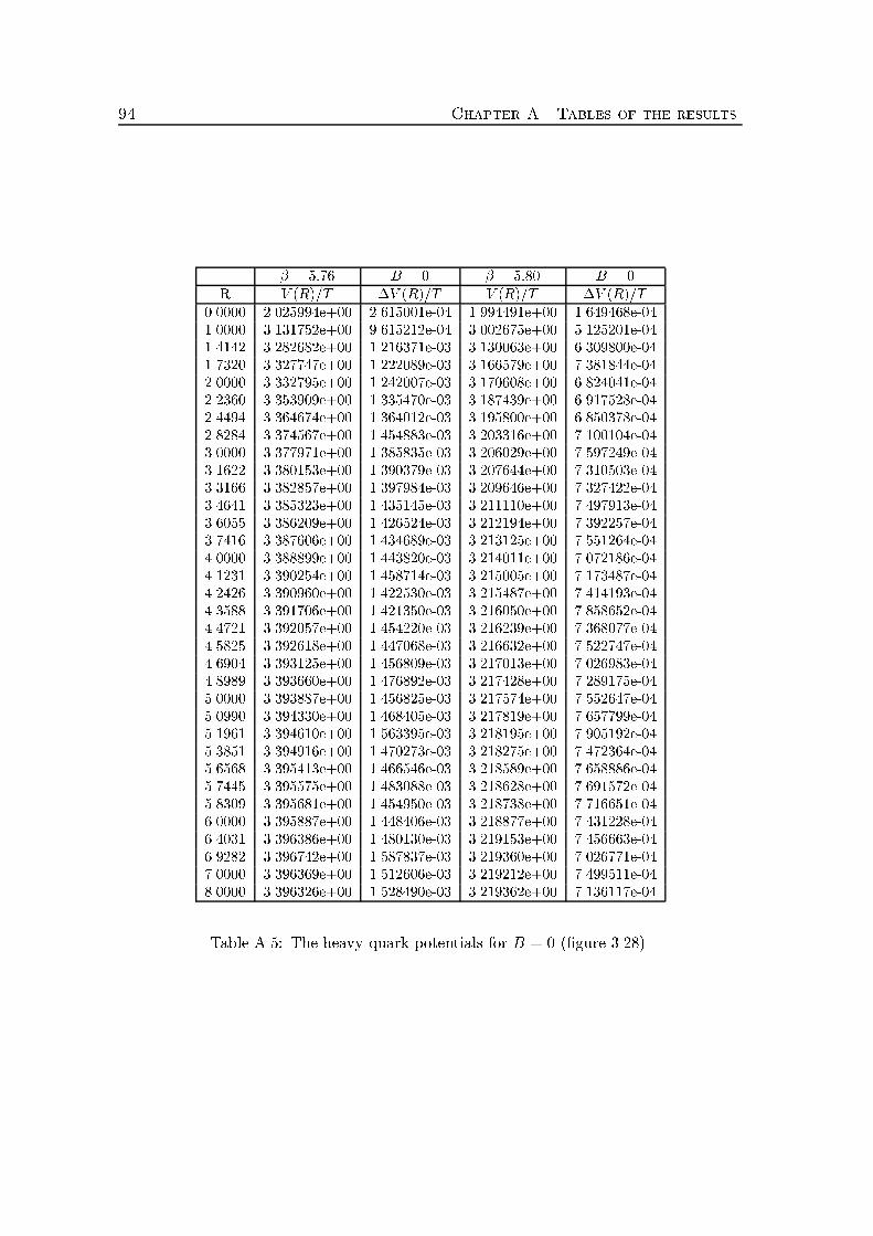
94 Chapter A. Tables of the results� = 5:76 B = 0 � = 5:80 B = 0R V (R)=T �V (R)=T V (R)=T �V (R)=T0.0000 2.025994e+00 2.615001e-04 1.994491e+00 1.649468e-041.0000 3.131752e+00 9.615212e-04 3.002675e+00 5.125201e-041.4142 3.282682e+00 1.216371e-03 3.130063e+00 6.309800e-041.7320 3.327747e+00 1.222089e-03 3.166579e+00 7.381844e-042.0000 3.332795e+00 1.242007e-03 3.170608e+00 6.824041e-042.2360 3.353909e+00 1.335470e-03 3.187439e+00 6.917528e-042.4494 3.364674e+00 1.364012e-03 3.195800e+00 6.850378e-042.8284 3.374567e+00 1.454883e-03 3.203316e+00 7.100104e-043.0000 3.377971e+00 1.385835e-03 3.206029e+00 7.597249e-043.1622 3.380153e+00 1.390379e-03 3.207644e+00 7.310503e-043.3166 3.382857e+00 1.397984e-03 3.209646e+00 7.327422e-043.4641 3.385323e+00 1.435145e-03 3.211110e+00 7.497913e-043.6055 3.386209e+00 1.426524e-03 3.212194e+00 7.392257e-043.7416 3.387606e+00 1.434689e-03 3.213125e+00 7.551264e-044.0000 3.388899e+00 1.443820e-03 3.214011e+00 7.072186e-044.1231 3.390254e+00 1.458714e-03 3.215005e+00 7.173487e-044.2426 3.390960e+00 1.422530e-03 3.215487e+00 7.414193e-044.3588 3.391706e+00 1.421350e-03 3.216050e+00 7.858652e-044.4721 3.392057e+00 1.454220e-03 3.216239e+00 7.368077e-044.5825 3.392618e+00 1.447068e-03 3.216632e+00 7.522747e-044.6904 3.393125e+00 1.456809e-03 3.217013e+00 7.026983e-044.8989 3.393660e+00 1.476892e-03 3.217428e+00 7.289175e-045.0000 3.393887e+00 1.456825e-03 3.217574e+00 7.552647e-045.0990 3.394330e+00 1.468405e-03 3.217819e+00 7.657799e-045.1961 3.394610e+00 1.563395e-03 3.218195e+00 7.905192e-045.3851 3.394916e+00 1.470273e-03 3.218275e+00 7.472364e-045.6568 3.395413e+00 1.466546e-03 3.218589e+00 7.658886e-045.7445 3.395575e+00 1.483088e-03 3.218628e+00 7.691572e-045.8309 3.395681e+00 1.454950e-03 3.218738e+00 7.716651e-046.0000 3.395887e+00 1.448406e-03 3.218877e+00 7.431228e-046.4031 3.396386e+00 1.480130e-03 3.219153e+00 7.456663e-046.9282 3.396742e+00 1.587837e-03 3.219360e+00 7.026771e-047.0000 3.396369e+00 1.512606e-03 3.219212e+00 7.499511e-048.0000 3.396326e+00 1.528490e-03 3.219362e+00 7.136117e-04Table A.5: The heavy quark potentials for B = 0 (�gure 3.28).

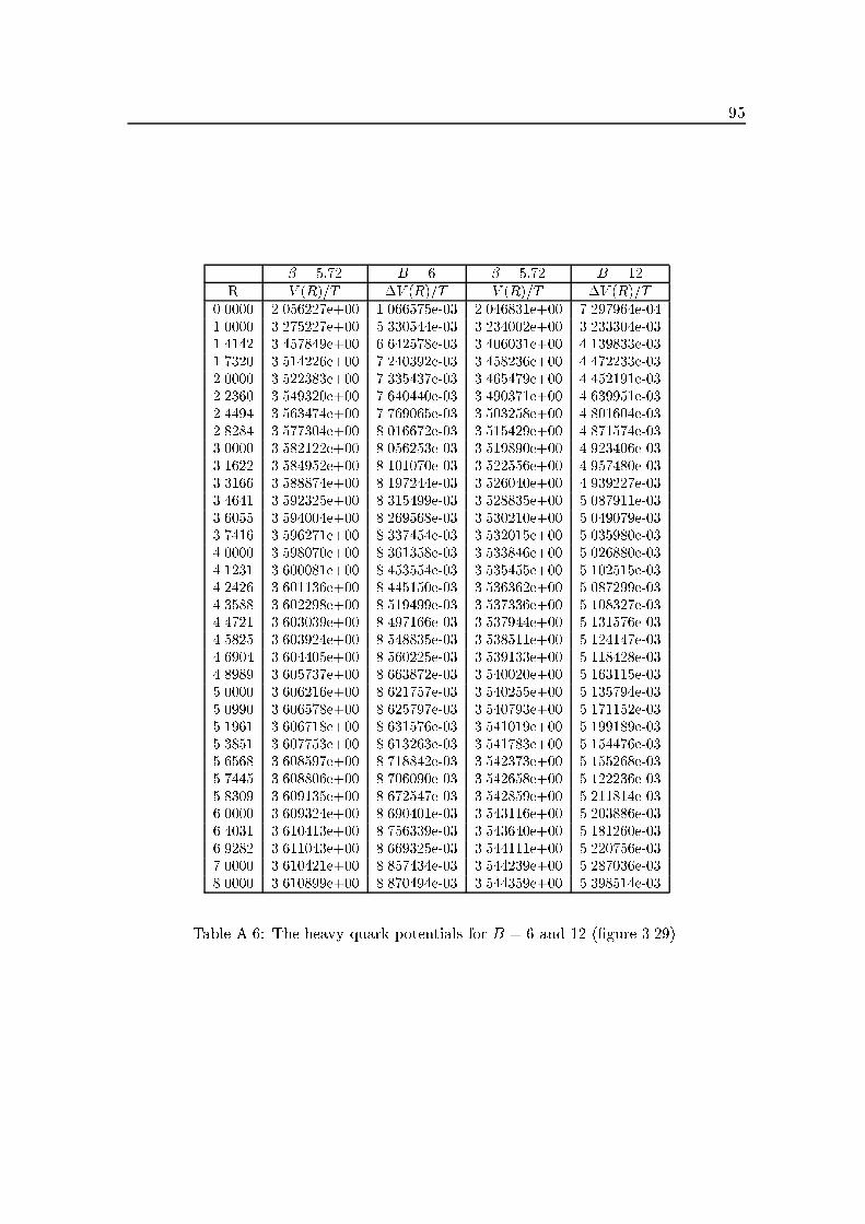
95� = 5:72 B = 6 � = 5:72 B = 12R V (R)=T �V (R)=T V (R)=T �V (R)=T0.0000 2.056227e+00 1.066575e-03 2.046831e+00 7.297964e-041.0000 3.275227e+00 5.330544e-03 3.234002e+00 3.233304e-031.4142 3.457849e+00 6.642578e-03 3.406031e+00 4.139833e-031.7320 3.514226e+00 7.240392e-03 3.458236e+00 4.472233e-032.0000 3.522383e+00 7.335437e-03 3.465479e+00 4.452191e-032.2360 3.549320e+00 7.640440e-03 3.490371e+00 4.639951e-032.4494 3.563474e+00 7.769065e-03 3.503258e+00 4.801604e-032.8284 3.577304e+00 8.016672e-03 3.515429e+00 4.871574e-033.0000 3.582122e+00 8.056253e-03 3.519890e+00 4.923406e-033.1622 3.584952e+00 8.101070e-03 3.522556e+00 4.957480e-033.3166 3.588874e+00 8.197244e-03 3.526040e+00 4.939227e-033.4641 3.592325e+00 8.315499e-03 3.528835e+00 5.087911e-033.6055 3.594004e+00 8.269568e-03 3.530210e+00 5.049079e-033.7416 3.596271e+00 8.337454e-03 3.532015e+00 5.035980e-034.0000 3.598070e+00 8.361358e-03 3.533846e+00 5.026880e-034.1231 3.600081e+00 8.453554e-03 3.535455e+00 5.102515e-034.2426 3.601136e+00 8.445150e-03 3.536362e+00 5.087299e-034.3588 3.602298e+00 8.519499e-03 3.537336e+00 5.108327e-034.4721 3.603039e+00 8.497166e-03 3.537944e+00 5.131576e-034.5825 3.603924e+00 8.548835e-03 3.538511e+00 5.124147e-034.6904 3.604405e+00 8.560225e-03 3.539133e+00 5.118428e-034.8989 3.605737e+00 8.663872e-03 3.540020e+00 5.163115e-035.0000 3.606216e+00 8.621757e-03 3.540255e+00 5.135794e-035.0990 3.606578e+00 8.625797e-03 3.540793e+00 5.171152e-035.1961 3.606718e+00 8.631576e-03 3.541019e+00 5.199189e-035.3851 3.607753e+00 8.613263e-03 3.541783e+00 5.154476e-035.6568 3.608597e+00 8.718842e-03 3.542373e+00 5.155268e-035.7445 3.608806e+00 8.706090e-03 3.542658e+00 5.122236e-035.8309 3.609135e+00 8.672547e-03 3.542859e+00 5.211814e-036.0000 3.609324e+00 8.690401e-03 3.543116e+00 5.203886e-036.4031 3.610413e+00 8.756339e-03 3.543640e+00 5.181260e-036.9282 3.611043e+00 8.669325e-03 3.544111e+00 5.220756e-037.0000 3.610421e+00 8.857434e-03 3.544239e+00 5.287036e-038.0000 3.610899e+00 8.870494e-03 3.544359e+00 5.398514e-03Table A.6: The heavy quark potentials for B = 6 and 12 (�gure 3.29).

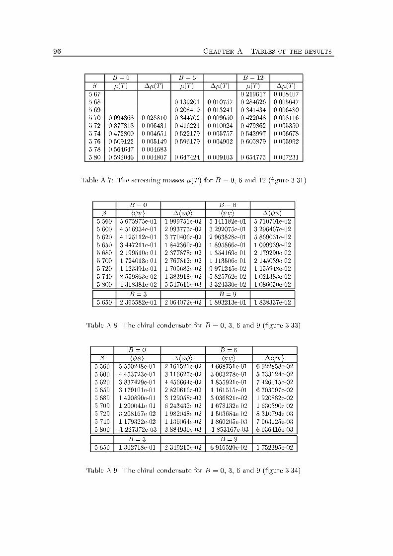
96 Chapter A. Tables of the resultsB = 0 B = 6 B = 12� �(T ) ��(T ) �(T ) ��(T ) �(T ) ��(T )5.67 0.219617 0.0084075.68 0.139201 0.010757 0.284626 0.0056475.69 0.208419 0.013241 0.341434 0.0064805.70 0.094868 0.028810 0.344702 0.009650 0.422048 0.0081165.72 0.377818 0.006431 0.416221 0.010024 0.479862 0.0053505.74 0.472800 0.004651 0.522179 0.005757 0.543997 0.0066785.76 0.509122 0.005149 0.596179 0.004902 0.605879 0.0059925.78 0.564647 0.0046835.80 0.592046 0.004807 0.647424 0.009103 0.654775 0.007231Table A.7: The screening masses �(T ) for B = 0, 6 and 12 (�gure 3.31)B = 0 B = 6� h � i �h � i h � i �h � i5.560 5.675975e-01 1.999751e-02 5.141182e-01 5.710701e-025.600 4.516934e-01 2.993775e-02 3.292075e-01 3.296467e-025.620 4.125112e-01 3.770406e-02 2.963828e-01 5.869031e-025.650 3.447211e-01 1.842360e-02 1.895866e-01 1.099939e-025.680 2.199510e-01 2.377878e-02 1.354169e-01 2.179290e-025.700 1.724013e-01 2.767812e-02 1.113506e-01 2.145039e-025.720 1.123391e-01 1.705682e-02 9.971245e-02 1.155948e-025.740 8.559863e-02 1.383918e-02 5.825762e-02 1.021383e-025.800 4.318381e-02 5.547616e-03 3.324330e-02 1.086050e-02B = 3 B = 95.650 2.395582e-01 2.064072e-02 1.893213e-01 1.838337e-02Table A.8: The chiral condensate for B = 0, 3, 6 and 9 (�gure 3.33)B = 0 B = 6� h � i �h � i h � i �h � i5.560 5.550248e-01 2.161521e-02 4.668751e-01 6.922858e-025.600 4.453723e-01 3.116627e-02 3.003278e-01 5.733124e-025.620 3.837429e-01 4.456664e-02 1.855921e-01 7.426015e-025.650 3.179101e-01 2.820616e-02 1.161515e-01 6.703597e-025.680 1.420890e-01 3.129058e-02 3.036821e-02 1.920882e-025.700 1.200041e-01 6.243432e-02 1.678132e-02 1.630390e-025.720 3.208167e-02 1.982048e-02 1.503684e-02 8.310794e-035.740 1.179322e-02 1.136064e-02 1.860205e-03 7.063125e-035.800 -1.227372e-03 3.884930e-03 -1.853167e-03 6.036416e-03B = 3 B = 95.650 1.302718e-01 2.349215e-02 6.916529e-02 1.752395e-02Table A.9: The chiral condensate for B = 0, 3, 6 and 9 (�gure 3.34)

Bibliography[1] J. Engels, O. Kaczmarek, F. Karsch, and E. Laermann, \The quenched limit oflattice QCD at non-zero baryon number", Nucl. Phys. B558 (1999) 307.[2] C. DeTar, O. Kaczmarek, F. Karsch, and E. Laermann, \String breaking in latticequantum chromodynamics", Phys. Rev. D59 (1999) 031501.[3] O. Kaczmarek, F. Karsch, E. Laermann, and M. L�utgemeier, \Heavy quarkpotentials in quenched QCD at high temperature", Phys. Rev. D62 (2000) 034021.[4] E. Laermann, C. DeTar, O. Kaczmarek, and F. Karsch, \String breaking in latticeQCD", Nucl. Phys. Proc. Suppl. 73 (1999) 447. 16th International Symposium onLattice Field Theory (LATTICE 98).[5] C. DeTar, O. Kaczmarek, F. Karsch, and E. Laermann, \The heavy-quark potentialin QCD at �nite temperature". In Copenhagen 1998, Strong and electroweakmatter.[6] J. Engels, O. Kaczmarek, F. Karsch, and E. Laermann, \The non-zero baryonnumber formulation of QCD", Nucl. Phys. Proc. Suppl. 83 (2000) 369{371. 17thInternational Symposium on Lattice Field Theory (LATTICE 99).[7] O. Kaczmarek, J. Engels, F. Karsch, and E. Laermann, \Lattice QCD at non-zerobaryon number". In Trento 1999, Understanding decon�nement in QCD.[8] H. J. Rothe, \Lattice gauge theories: An introduction". Singapore, Singapore:World Scienti�c (1992) 381 p.[9] I. Montvay and G. M�unster, \Quantum �elds on a lattice". Cambridge, UK: Univ.Pr. (1994) 491 p. (Cambridge monographs on mathematical physics).[10] H. Meyer-Ortmanns, \Phase transitions in quantum chromodynamics", Rev. Mod.Phys. 68 (1996) 473{598.[11] M. Fukugita, M. Okawa, and A. Ukawa, \Finite size scaling study of the decon�ningphase transition in pure SU(3) lattice gauge theory", Nucl. Phys. B337 (1990) 181.[12] A. Peikert, \QCD thermodynamics with 2+1 quark avours in lattice simulations",Ph.D. Thesis Bielefeld (2000). 97

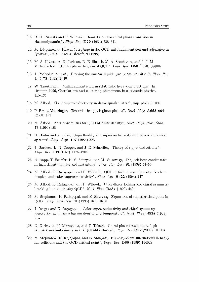
98 Bibliography[13] R. D. Pisarski and F. Wilczek, \Remarks on the chiral phase transition inchromodynamics", Phys. Rev. D29 (1984) 338{341.[14] M. L�utgemeier, \Phasen�uberg�ange in der QCD mit fundamentalen und adjungiertenQuarks", Ph.D. Thesis Bielefeld (1998).[15] M. A. Halasz, A. D. Jackson, R. E. Shrock, M. A. Stephanov, and J. J. M.Verbaarschot, \On the phase diagram of QCD", Phys. Rev. D58 (1998) 096007.[16] J. Pochodzalla et al., \Probing the nuclear liquid - gas phase transition", Phys. Rev.Lett. 75 (1995) 1040.[17] W. Trautmann, \Multifragmentation in relativistic heavy-ion reactions". InDronten 1996, Correlations and clustering phenomena in subatomic physics,115-135.[18] M. Alford, \Color superconductivity in dense quark matter", hep-ph/0003185.[19] P. Braun-Munzinger, \Towards the quark-gluon plasma", Nucl. Phys. A663-664(2000) 183.[20] M. Alford, \New possibilities for QCD at �nite density", Nucl. Phys. Proc. Suppl.73 (1999) 161.[21] D. Bailin and A. Love, \Super uidity and superconductivity in relativistic fermionsystems", Phys. Rept. 107 (1984) 325.[22] J. Bardeen, L. N. Cooper, and J. R. Schrie�er, \Theory of superconductivity",Phys. Rev. 108 (1957) 1175{1204.[23] R. Rapp, T. Sch�afer, E. V. Shuryak, and M. Velkovsky, \Diquark bose condensatesin high density matter and instantons", Phys. Rev. Lett. 81 (1998) 53{56.[24] M. Alford, K. Rajagopal, and F. Wilczek, \QCD at �nite baryon density: Nucleondroplets and color superconductivity", Phys. Lett. B422 (1998) 247.[25] M. Alford, K. Rajagopal, and F. Wilczek, \Color- avor locking and chiral symmetrybreaking in high density QCD", Nucl. Phys. B537 (1999) 443.[26] M. Stephanov, K. Rajagopal, and E. Shuryak, \Signatures of the tricritical point inQCD", Phys. Rev. Lett. 81 (1998) 4816{4819.[27] J. Berges and K. Rajagopal, \Color superconductivity and chiral symmetryrestoration at nonzero baryon density and temperature", Nucl. Phys. B538 (1999)215.[28] O. Kiriyama, M. Maruyama, and F. Takagi, \Chiral phase transition at hightemperature and density in the QCD-like theory", Phys. Rev. D62 (2000) 105008.[29] M. Stephanov, K. Rajagopal, and E. Shuryak, \Event-by-event uctuations in heavyion collisions and the QCD critical point", Phys. Rev. D60 (1999) 114028.

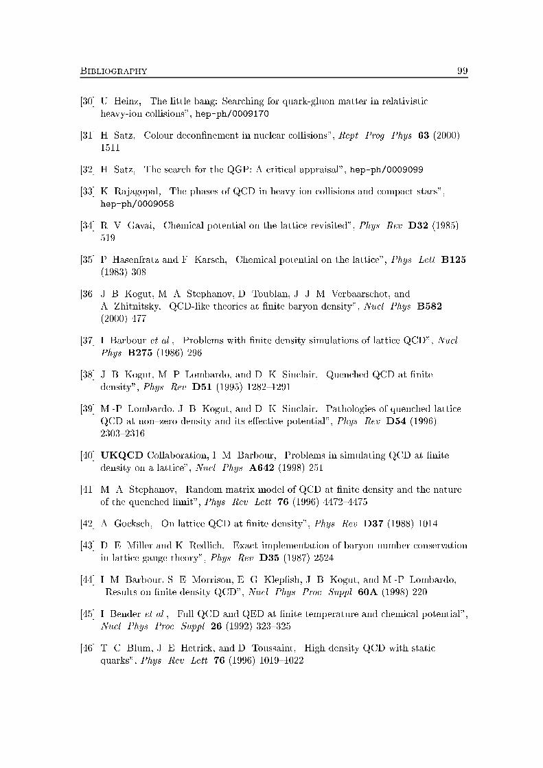
Bibliography 99[30] U. Heinz, \The little bang: Searching for quark-gluon matter in relativisticheavy-ion collisions", hep-ph/0009170.[31] H. Satz, \Colour decon�nement in nuclear collisions", Rept. Prog. Phys. 63 (2000)1511.[32] H. Satz, \The search for the QGP: A critical appraisal", hep-ph/0009099.[33] K. Rajagopal, \The phases of QCD in heavy ion collisions and compact stars",hep-ph/0009058.[34] R. V. Gavai, \Chemical potential on the lattice revisited", Phys. Rev. D32 (1985)519.[35] P. Hasenfratz and F. Karsch, \Chemical potential on the lattice", Phys. Lett. B125(1983) 308.[36] J. B. Kogut, M. A. Stephanov, D. Toublan, J. J. M. Verbaarschot, andA. Zhitnitsky, \QCD-like theories at �nite baryon density", Nucl. Phys. B582(2000) 477.[37] I. Barbour et al., \Problems with �nite density simulations of lattice QCD", Nucl.Phys. B275 (1986) 296.[38] J. B. Kogut, M. P. Lombardo, and D. K. Sinclair, \Quenched QCD at �nitedensity", Phys. Rev. D51 (1995) 1282{1291.[39] M.-P. Lombardo, J. B. Kogut, and D. K. Sinclair, \Pathologies of quenched latticeQCD at non{zero density and its e�ective potential", Phys. Rev. D54 (1996)2303{2316.[40] UKQCD Collaboration, I. M. Barbour, \Problems in simulating QCD at �nitedensity on a lattice", Nucl. Phys. A642 (1998) 251.[41] M. A. Stephanov, \Random matrix model of QCD at �nite density and the natureof the quenched limit", Phys. Rev. Lett. 76 (1996) 4472{4475.[42] A. Gocksch, \On lattice QCD at �nite density", Phys. Rev. D37 (1988) 1014.[43] D. E. Miller and K. Redlich, \Exact implementation of baryon number conservationin lattice gauge theory", Phys. Rev. D35 (1987) 2524.[44] I. M. Barbour, S. E. Morrison, E. G. Klep�sh, J. B. Kogut, and M.-P. Lombardo,\Results on �nite density QCD", Nucl. Phys. Proc. Suppl. 60A (1998) 220.[45] I. Bender et al., \Full QCD and QED at �nite temperature and chemical potential",Nucl. Phys. Proc. Suppl. 26 (1992) 323{325.[46] T. C. Blum, J. E. Hetrick, and D. Toussaint, \High density QCD with staticquarks", Phys. Rev. Lett. 76 (1996) 1019{1022.

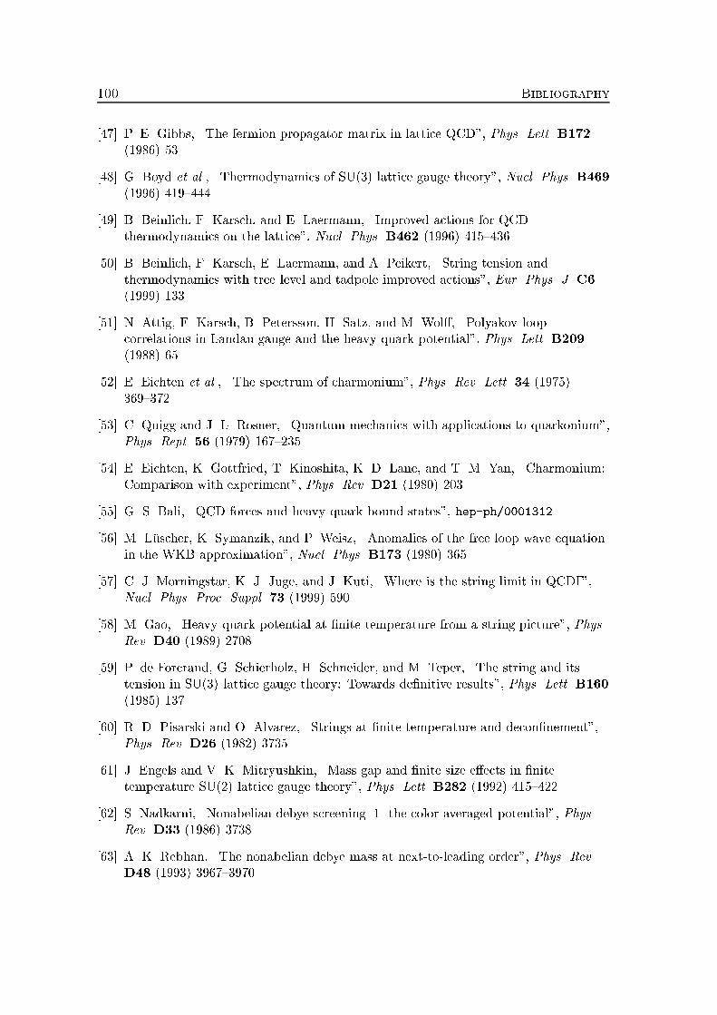
100 Bibliography[47] P. E. Gibbs, \The fermion propagator matrix in lattice QCD", Phys. Lett. B172(1986) 53.[48] G. Boyd et al., \Thermodynamics of SU(3) lattice gauge theory", Nucl. Phys. B469(1996) 419{444.[49] B. Beinlich, F. Karsch, and E. Laermann, \Improved actions for QCDthermodynamics on the lattice", Nucl. Phys. B462 (1996) 415{436.[50] B. Beinlich, F. Karsch, E. Laermann, and A. Peikert, \String tension andthermodynamics with tree level and tadpole improved actions", Eur. Phys. J. C6(1999) 133.[51] N. Attig, F. Karsch, B. Petersson, H. Satz, and M. Wol�, \Polyakov loopcorrelations in Landau gauge and the heavy quark potential", Phys. Lett. B209(1988) 65.[52] E. Eichten et al., \The spectrum of charmonium", Phys. Rev. Lett. 34 (1975)369{372.[53] C. Quigg and J. L. Rosner, \Quantum mechanics with applications to quarkonium",Phys. Rept. 56 (1979) 167{235.[54] E. Eichten, K. Gottfried, T. Kinoshita, K. D. Lane, and T. M. Yan, \Charmonium:Comparison with experiment", Phys. Rev. D21 (1980) 203.[55] G. S. Bali, \QCD forces and heavy quark bound states", hep-ph/0001312.[56] M. L�uscher, K. Symanzik, and P. Weisz, \Anomalies of the free loop wave equationin the WKB approximation", Nucl. Phys. B173 (1980) 365.[57] C. J. Morningstar, K. J. Juge, and J. Kuti, \Where is the string limit in QCD?",Nucl. Phys. Proc. Suppl. 73 (1999) 590.[58] M. Gao, \Heavy quark potential at �nite temperature from a string picture", Phys.Rev. D40 (1989) 2708.[59] P. de Forcrand, G. Schierholz, H. Schneider, and M. Teper, \The string and itstension in SU(3) lattice gauge theory: Towards de�nitive results", Phys. Lett. B160(1985) 137.[60] R. D. Pisarski and O. Alvarez, \Strings at �nite temperature and decon�nement",Phys. Rev. D26 (1982) 3735.[61] J. Engels and V. K. Mitryushkin, \Mass gap and �nite size e�ects in �nitetemperature SU(2) lattice gauge theory", Phys. Lett. B282 (1992) 415{422.[62] S. Nadkarni, \Nonabelian debye screening. 1. the color averaged potential", Phys.Rev. D33 (1986) 3738.[63] A. K. Rebhan, \The nonabelian debye mass at next-to-leading order", Phys. Rev.D48 (1993) 3967{3970.

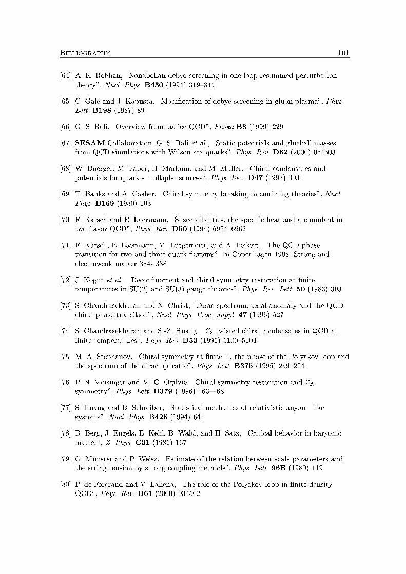
Bibliography 101[64] A. K. Rebhan, \Nonabelian debye screening in one loop resummed perturbationtheory", Nucl. Phys. B430 (1994) 319{344.[65] C. Gale and J. Kapusta, \Modi�cation of debye screening in gluon plasma", Phys.Lett. B198 (1987) 89.[66] G. S. Bali, \Overview from lattice QCD", Fizika B8 (1999) 229.[67] SESAM Collaboration, G. S. Bali et al., \Static potentials and glueball massesfrom QCD simulations with Wilson sea quarks", Phys. Rev. D62 (2000) 054503.[68] W. Buerger, M. Faber, H. Markum, and M. Muller, \Chiral condensates andpotentials for quark - multiplet sources", Phys. Rev. D47 (1993) 3034.[69] T. Banks and A. Casher, \Chiral symmetry breaking in con�ning theories", Nucl.Phys. B169 (1980) 103.[70] F. Karsch and E. Laermann, \Susceptibilities, the speci�c heat and a cumulant intwo avor QCD", Phys. Rev. D50 (1994) 6954{6962.[71] F. Karsch, E. Laermann, M. L�utgemeier, and A. Peikert, \The QCD phasetransition for two and three quark avours". In Copenhagen 1998, Strong andelectroweak matter 384- 388.[72] J. Kogut et al., \Decon�nement and chiral symmetry restoration at �nitetemperatures in SU(2) and SU(3) gauge theories", Phys. Rev. Lett. 50 (1983) 393.[73] S. Chandrasekharan and N. Christ, \Dirac spectrum, axial anomaly and the QCDchiral phase transition", Nucl. Phys. Proc. Suppl. 47 (1996) 527.[74] S. Chandrasekharan and S.-Z. Huang, \Z3 twisted chiral condensates in QCD at�nite temperatures", Phys. Rev. D53 (1996) 5100{5104.[75] M. A. Stephanov, \Chiral symmetry at �nite T, the phase of the Polyakov loop andthe spectrum of the dirac operator", Phys. Lett. B375 (1996) 249{254.[76] P. N. Meisinger and M. C. Ogilvie, \Chiral symmetry restoration and ZNsymmetry", Phys. Lett. B379 (1996) 163{168.[77] S. Huang and B. Schreiber, \Statistical mechanics of relativistic anyon - likesystems", Nucl. Phys. B426 (1994) 644.[78] B. Berg, J. Engels, E. Kehl, B. Waltl, and H. Satz, \Critical behavior in baryonicmatter", Z. Phys. C31 (1986) 167.[79] G. M�unster and P. Weisz, \Estimate of the relation between scale parameters andthe string tension by strong coupling methods", Phys. Lett. 96B (1980) 119.[80] P. de Forcrand and V. Laliena, \The role of the Polyakov loop in �nite densityQCD", Phys. Rev. D61 (2000) 034502.

102 Bibliography[81] N. Cabibbo and E. Marinari, \A new method for updating SU(N) matrices incomputer simulations of gauge theories", Phys. Lett. B119 (1982) 387.[82] K. Fabricius and O. Haan, \Heat bath method for the twisted Eguchi-Kawaimodel", Phys. Lett. B143 (1984) 459.[83] A. D. Kennedy and B. J. Pendleton, \Improved heat bath method for Monte Carlocalculations in lattice gauge theories", Phys. Lett. B156 (1985) 393.[84] S. L. Adler, \An overrelaxation method for the Monte Carlo evaluation of thepartition function for multiquadratic actions", Phys. Rev. D23 (1981) 2901.[85] R. Brower, P. Rossi, and C.-I. Tan, \The external �eld problem for QCD", Nucl.Phys. B190 (1981) 699.[86] G. Parisi, R. Petronzio, and F. Rapuano, \A measurement of the string tension nearthe continuum limit", Phys. Lett. B128 (1983) 418.[87] P. D. Forcrand and C. Roiesnel, \Re�ned methods for measuring large distancecorrelations", Phys. Lett. B151 (1985) 77.[88] A. Ukawa, \QCD phase transitions at �nite temperatures", Nucl. Phys. Proc. Suppl.17 (1990) 118{136.[89] G. S. Bali and K. Schilling, \Running coupling and the lambda parameter fromSU(3) lattice simulations", Phys. Rev. D47 (1993) 661{672.[90] C. Bernard et al., \The Nt = 6 equation of state for two avor QCD", Nucl. Phys.Proc. Suppl. 47 (1996) 503.[91] MILC Collaboration, C. Bernard et al., \The equation of state for two avor QCDat n(t) = 6", Phys. Rev. D55 (1997) 6861{6869.[92] W. Sakuler et al., \Chiral symmetry and charge density in mesons for Kogut-Susskind and Wilson fermions", Phys. Lett. B276 (1992) 155{162.[93] I. T. Drummond, \Strong coupling model for string breaking on the lattice", Phys.Lett. B434 (1998) 92{98.[94] O. Philipsen and H. Wittig, \String breaking in non-abelian gauge theories withfundamental matter �elds", Phys. Rev. Lett. 81 (1998) 4056{4059.[95] ALPHA Collaboration, F. Knechtli and R. Sommer, \String breaking in SU(2)gauge theory with scalar matter �elds", Phys. Lett. B440 (1998) 345{352.[96] F. Karsch and S. Stickan, \The three-dimensional, three-state Potts model in anexternal �eld", Phys. Lett. B488 (2000) 319.[97] K. Rummukainen, M. Tsypin, K. Kajantie, M. Laine, and M. Shaposhnikov, \Theuniversality class of the electroweak theory", Nucl. Phys. B532 (1998) 283.

Bibliography 103[98] N. Wilding and A. Bruce, \Density uctuations and �eld mixing in the critical uid", J. Phys.: Cond.Matter 4 (1992) 3087.[99] N. Wilding, \Simulation studies of uid critical behavior", cond-mat/9610133(1996).

104 Bibliography

Hiemit erkl�are ich, dass diese Arbeit von mir pers�onlich angefertigt wurde und nur dieangegebenen Hilfsmittel verwendet wurden.Olaf Kaczmarek

105