cei ipps99

7/30/2019 Cei Ipps99

http://slidepdf.com/reader/full/cei-ipps99 1/25

On the Design and Evaluation of Job Scheduling

Algorithms

Jochen Krallmann, Uwe Schwiegelshohn, and Ramin Yahyapour

Computer Engineering InstituteUniversity Dortmund

44221 Dortmund, Germanyhttp://www-ds.e-technik.uni-dortmund.de{uwe,yahya}@ds.e-technik.uni-dortmund.de

Abstract. In this paper we suggest a strategy to design job schedul-ing systems. To this end, we first split a scheduling system into threecomponents: Scheduling policy, objective function and scheduling algo-rithm. After discussing the relationship between those components weexplain our strategy with the help of a simple example. The main focusof this example is the selection and the evaluation of several schedulingalgorithms.

1 Introduction

Job scheduling for processors is a complex task. This is especially true for mas-sively parallel processors (MPPs) where many users with a multitude of different jobs share a large amount of system resources. While job scheduling does not af-fect the results of a job, it may have a significant influence on the efficiency of thesystem. For instance, a good job scheduling system may reduce the number of MPP nodes that are required to process a certain amount of jobs within a giventime frame or it may permit more users or jobs to use the resources of a machine.Therefore, the job scheduling system is an important part in the managementof computer resources which frequently represent a significant investment for acompany or institution in the case of MPPs.

Hence, the availability of a good job scheduling system is in the interest of the owner or administrator of an MPP. It is therefore not surprising that in thepast new job scheduling methods have been frequently introduced by institutionswhich were among the first owners of MPPs like, for instance, ANL [10], CTC [11]or NASA Ames [12]. On the other hand, some machine manufacturers showedonly limited interest in this issue as they frequently seem to have the opinion

that “machines are not sold because of superior job schedulers”. Moreover, thedesign of a job scheduling system must be based on the specific environment of a parallel system as we will argue in this paper. Consequently, administrators of MPPs will remain to be involved in the design of job scheduling systems in thefuture. Methods or at least guidelines for the selection and evaluation of such a

Supported by the NRW Metacomputing grant

7/30/2019 Cei Ipps99


system would therefore be beneficial. It is the goal of this paper to make a firsta step into this direction.

We start this paper by taking a close look at job scheduling systems. For ussuch is system is divided into 3 components: Scheduling policy, objective functionand scheduling algorithm. We discuss those components and the dependencesbetween them. In the second part of the paper we use a simple example todescribe the process of scheduling algorithm selection and evaluation. We donot believe that there is a single scheduling algorithm that suits all systems.Therefore, it is not the purpose of this example to show the superiority of anyparticular algorithm but to illustrate a method for the design of schedulingsystems.

2 Scheduling Systems

The scheduling system of a multiprocessor receives a stream of job submissiondata and produces a valid schedule. We use the term ‘stream’ to indicate thatsubmission data for different jobs need not arrive at the same time. Also thearrival of any specific data is not necessarily predictable, that is, the schedulingsystem may not be aware of any data arriving in the future. Therefore, thescheduling system must deal with a so called ‘on-line’ behavior.

Further, we do not specify the amount and the type of job submission data.Different scheduling systems may accept or require different sets of submissiondata. For us submission data comprise all data which are used to determine aschedule. However, a few different categories can be distinguished:

– User Data: These data may be used to determine job priorities. For in-stance, the jobs of some user may receive faster service at a specific location

while other jobs are only accepted if sufficient resources are available.– Resource Requests: These data specify the resources which are requested

for a job. Often they include the number and the type of processors, theamount of memory as well as some specific hardware and software require-ments. Some of these data may be estimates, like the execution time of a job, or describe a range of acceptable values, like the number of processorsfor a malleable job.

– Scheduling Ob jectives: These data may help the scheduling system togenerate ‘good’ schedules. For instance, a user may state that she needs theresult by 8am the next morning while an earlier job completion will be of nobenefit to her. Other users may be willing to pay more if they obtain theirresults within the next hour.

Of course other submission data are possible as well. Job submission dataare entered by the user and typically provided to the system when a job issubmitted for execution. However, some systems may also allow reservation of resources before the actual job submission. Such a feature is especially beneficialfor multisite metacomputing [17]. In addition, technical data are often requiredto start a job, like the name and the location of the input data files of the job.

7/30/2019 Cei Ipps99


But as these data do not affect the schedule if they are correct, we ignore themhere. Finally note that the submission of erroneous or incorrect data is also

possible. However, in this case a job may be immediately rejected or fail to run.Now, we take a closer look at the schedule. A schedule is an allocation of

system resources to individual jobs for certain time periods. Therefore, a schedulecan be described by providing all the time instances where a change of resourceallocation occurs as long as either this change is initiated by the schedulingsystem or the scheduling system is notified of this change. To illustrate thisrestriction assume a job being executed on a processor that is also busy with someoperating system tasks. Here, we do not consider changes of resource allocationwhich are due to the context switches between OS tasks and the application.Those changes are managed by the system software without any involvement of our scheduling system.

For a schedule to be valid some restrictions of the hardware and the systemsoftware must be observed. For instance, a parallel processor system may notsupport gang scheduling or require that at most one application is active on aspecific processor at any time. Therefore, the validity constraints of a scheduleare defined by the target machine. We assume that a scheduling system doesnot attempt to produce an invalid schedule. However, note that the validity of aschedule is not affected by the properties of a submitted job as those propertiesare not guaranteed to comply with submission data. For instance, if not enoughmemory is requested from and assigned to a job, the job will simply fail to run.But this does not mean that the resulting schedule is invalid. Also, a scheduledepends upon other influences which cannot be controlled by the schedulingsystem, like the sudden failure of a hardware component. Therefore, the finalschedule is only available after the execution of all jobs.

Next, the scheduling system is divided into 3 parts:

1. A scheduling policy ,2. an objective function and3. a scheduling algorithm .

In the rest of this section we first describe these parts separately. Then thedependences between them are discussed. Finally, we compare the evaluation of scheduling systems with the evaluation of computer architectures.

2.1 Scheduling Policy

The scheduling policy forms the top level of a scheduling system. It is defined bythe owner or administrator of a machine. In general, the scheduling strategy is a

collection of rules to determine the resource allocation if not enough resources areavailable to satisfy all requests immediately. To better illustrate our approach,we give an example:

Example 1. The department of chemistry at University A has bought a paral-lel computer which was financed to a large part by the drug design lab. Thedepartment establishes the following rules for the use of the machine:

7/30/2019 Cei Ipps99


1. All jobs from the drug design lab have the highest priority and must beexecuted as soon as possible.

2. 100 GB of secondary storage is reserved for data from the drug design lab.3. Applications from the whole university are accepted but the labs of thechemistry department have preferred access.

4. Some computation time is sold to cooperation partners from the chemicalindustry in order to pay for machine maintenance and software upgrades.

5. Some computation time is also made available to the theoretical chemistrylab course during their scheduled hours.

Note that these rules are hardly detailed enough to generate a schedule. Butthey allow a fuzzy distinction between good and bad schedules. Also, there may besome additional general rules which are not explicitly mentioned, like ‘Completeall applications as soon as possible if this does not contradict any other rule’.Finally, some conflicts between those rules may occur and must be resolved. For

instance in Example 1, some jobs from the drug design lab may compete withthe theoretical chemistry lab course. Hence, in our view a good scheduling policyhas the following two properties:

1. It contains rules to resolve conflicts between other rules if those conflictsmay occur.

2. It can be implemented.

We believe that there is no general method to derive a scheduling policy. Alsothere is no need to provide a very detailed policy with clearly defined quotas.In many cases this will result in a reduction of the number of good schedules.For instance, it would not be helpful at this point to demand that 5% of thecomputation time is sold to the chemical industry in Example 1. If there are only

a few jobs from the drug design lab then the department would be able to earnmore money by defining a higher industry quota. Otherwise, the departmentmust decide whether to obtain other funding for the machine maintenance or toreduce the priority of some jobs of the drug design lab. This issue will be furtherdiscussed in Section 2.4.

2.2 Objective Function

As stated in the previous section the owner of a machine will be able to determinewhether any given schedule is good or bad . However, it is the goal of a schedulingsystem to consistently produce schedules which are as good as possible. Thisleads to two problems:

1. It must be demonstrated that the scheduling system will always producegood schedules.

2. It is necessary to provide a ranking among good schedules.

Problems of the first kind are addressed in theoretical computer science bythe concept of competitive analysis, see [18]. Unfortunately, this approach is notapplicable for our scheduling systems for the following reasons:

7/30/2019 Cei Ipps99


– Often competitive analysis cannot be successfully applied to methods whichare based on very complex algorithms or which use specific input data sets.

– Competitive factors are worst case factors that frequently are not acceptablein practice. For instance, a competitive factor of 2 for the machine load of aschedule denotes that in some cases 50% of the resources are not used. Onthe other hand, those worst case input data typically do not occur in realinstallations. Frequently, this is also true if randomization is used for theanalysis.

Alternatively, a scheduling system can be applied to a multitude of differentstreams of submission data and the resulting schedules can be evaluated. Thisrequires a method to automatically determine the quality of a schedule. There-fore, an objective function must be defined that assigns a scalar value, the socalled schedule cost , to each schedule. Note that this property is essential for themechanical evaluation and ranking of a schedule. In the simplest case all good

schedules are mapped to 0 while all bad schedules obtain the value 1. Most likelyhowever, this kind of objective function will be of little help. To derive a suitableobjective function an approach based on multi criteria optimization can be used,see e.g. [20]:

1. For a typical set of jobs determine the Pareto-optimal schedules based onthe scheduling policy.

2. Define a partial order of these schedules.3. Derive an objective function that generates this order.4. Repeat this process for other sets of jobs and refine the ob jective function

accordingly.

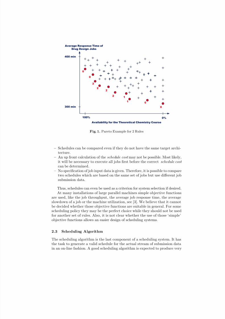
To illustrate Steps 1 and 2 of our approach we consider Rules 1 and 5 of

Example 1. Assume that both rules are conflicting for the chosen set of jobsubmission data. Therefore, we determine a variety of different schedules, seeFig. 1. Note that we are not biased toward any specific algorithm in this step.We are primarily interested in those schedules which are good with respect to atleast one criterion. Therefore, at first all Pareto-optimal schedules are selected.Those schedules are indicated by bullets in Fig. 1. Next, a partial order of thePareto-optimal schedules is obtained by applying additional conflict resolvingrules or by asking the owner. In the example of Fig. 1 numbers 0, 1 and 2 havebeen assigned to the Pareto-optimal schedules in order to indicate the desiredpartial order. Here any schedule 1 is superior to any schedule 0 and inferior toany schedule 2 while the order among all schedules 1 does not matter.

The approach is based on the availability of a few typical sets of job data.Further, it is assumed that each rule of the scheduling policy are associated withsingle criterion functions, like Rule 4 of Example 1 with the function ‘amount of computation time allocated to jobs from the cooperation partners from industry’.If this is not the case, complex rules must be split.

Now, it is possible to compare different schedules if the same objective func-tion and the same set of jobs is used. Further, there are a few additional aspectswhich are also noteworthy:

7/30/2019 Cei Ipps99


7/30/2019 Cei Ipps99


Achievable by online algorithms

Average Response Time

of Drug Design Jobs

Availability for the Theoretical Chemistry Course

100% 0%

600 min

300 min

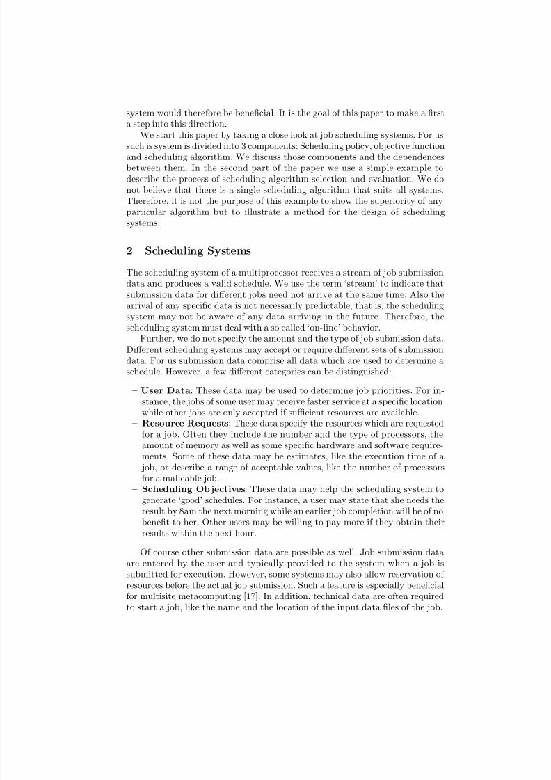
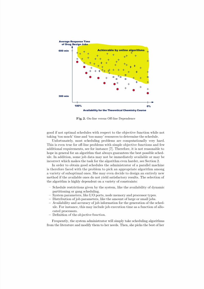
Fig. 2. On-line versus Off-line Dependence

good if not optimal schedules with respect to the objective function while nottaking ‘too much’ time and ‘too many’ resources to determine the schedule.

Unfortunately, most scheduling problems are computationally very hard.This is even true for off-line problems with simple objective functions and fewadditional requirements, see for instance [7]. Therefore, it is not reasonable to

hope in general for an algorithm that always guarantees the best possible sched-ule. In addition, some job data may not be immediately available or may beincorrect which makes the task for the algorithm even harder, see Section 2.

In order to obtain good schedules the administrator of a parallel machineis therefore faced with the problem to pick an appropriate algorithm amonga variety of suboptimal ones. She may even decide to design an entirely newmethod if the available ones do not yield satisfactory results. The selection of the algorithm is highly dependent on a variety of constraints:

– Schedule restrictions given by the system, like the availability of dynamicpartitioning or gang scheduling.

– System parameters, like I/O ports, node memory and processor types.– Distribution of job parameters, like the amount of large or small jobs.

– Availability and accuracy of job information for the generation of the sched-ule. For instance, this may include job execution time as a function of allo-cated processors.

– Definition of the ob jective function.

Frequently, the system administrator will simply take scheduling algorithmsfrom the literature and modify them to her needs. Then, she picks the best of her

7/30/2019 Cei Ipps99


algorithm candidates. After making sure that her algorithm of choice actuallygenerate valid schedules, she also must decide whether it makes sense to look for

a better algorithm. Therefore, it is necessary to evaluate those algorithms. Wedistinguish the following methods of evaluation:

1. Evaluation using algorithmic theory2. Simulation with job data derived from

– an actual workload– a workload model

In general theoretical evaluation is not well suited for our scheduling algorithmsas already discussed in Section 2.2. Occasionally, this method is used to deter-mine lower bounds for schedules. These lower bounds can provide an estimate fora potential improvement of the schedule by switching to a different algorithm.However, it is very difficult to find suitable lower bounds for complex objective

functions.Alternatively, an algorithm can be fed with a stream of job submission data.

The actual schedule and its cost are determined by simulation with the help of the complete set of job data. The procedure is repeated with a large number of input data sets. The reliability of this method depends on several factors:

– Availability of correct job data– Compliance of the used job set with the job set on the target machine

Actual workload data can be used if they are recorded on a machine with auser group such that sufficient similarity exists with the target machine and itsusers. This is relatively easy if traces from the target machine and the target user

community are available. Otherwise some traces must be obtained from othersources, see e.g. [1]. In this case it is necessary to check whether the workloadtrace is suitable. This may even require some modifications of the trace.

Also note that the trace only contains job data of a specific schedule. In an-other schedule these job data may not be valid as is demonstrated in Examples 2and 3:

Example 2. Assume a parallel processor that uses a single bus for communica-tion. Here, independent jobs compete for the communication resource. Therefore,the actual performance of job i depends on the jobs executed concurrently with job i.

Example 3. Assume a machine and a scheduling system that support adaptive

partitioning. In this case, the number of resources allocated to job i again de-pends on other jobs executed concurrently with job i.

Also, a comprehensive evaluation of an algorithm frequently requires a largeamount of input data that available workload traces may not be able to provide.

If accurate workload data are not available then artificial data must be gen-erated. To this end a workload model is used. Again conformity with future real

7/30/2019 Cei Ipps99


job data is essential and must be verified. On the other hand, this approach isable to overcome some of the problems associated with trace data simulation,

if the workload model is precise enough. For a more detailed discussion of thissubject, see also [3].

Unfortunately, it cannot be expected that a single scheduling algorithm willproduce a better schedule than any other method for all used input data sets. Inaddition the resource consumption of the various algorithms may be different.Therefore, the process of picking the best suited algorithm may again requiresome form of multi criteria optimization.

2.4 Dependences

The main dependence stream between the components of a scheduling systemis easy to see: The scheduling policy produces rules which are used to derivean objective function. The application of this objective function to a scheduleyields the schedule cost which allows performance measurements for the variousalgorithms. However, there are also additional dependences. For instance, somepolicy rules may not allow efficient scheduling algorithms, see Example 4.

Example 4. Assume a machine that does not support time sharing. The schedul-ing policy includes the rule:

Every weekday at 10am the entire machine must be available to a theoreticalchemistry class for 1 hour.

The Pareto-optimal schedules used for the determination of the objectivefunction show an acceptable (by the owner) amount of idle resources before10am. However, as users are not able to provide accurate execution time esti-mates for their jobs no scheduling algorithm can generate good schedules.

Such a situation is shown in Fig. 2 for Example 1. There, it is assumed thaton-line algorithms cover a significantly smaller area of schedules than off-linemethods with complete job knowledge. This may require a review of the conflictresolving strategy and thus affect the schedule cost. Unfortunately, this on-linearea of schedules will typically be the result of a combination of several on-linealgorithms. Therefore, the off-line methods in the approach of Section 2.2 cannotbe simply replaced by a single or a few on-line algorithms. In addition, a suitableon-line algorithm may not be available at this time.

More of these additional dependences are listed below:

– Too many or too restrictive policy rules may prevent acceptable schedulesat all.

– There may not be sufficient rules to discriminate betweengood

andbad

sched-ules as some implicitly assumed rules are not explicitly stated.– While there may be a variety of different objective functions which all sup-

port the policy rules, a specific objective function may not be suitable as acriterion for an on-line scheduling algorithm.

– The workload model may not be correct if users adapt their submissionpattern due to their knowledge of the policy rules.

7/30/2019 Cei Ipps99


– The workload model must be modified as the number of users and/or thetypes and sizes of submitted jobs change over time.

Due to these dependences a few design iterations may be required to deter-mine the best suitable scheduling algorithms and/or it may be appropriate torepeat the design process occasionally.

2.5 Comparison

In this section we briefly compare the evaluation of scheduling systems withthe well known procedure used for computer architectures. Today, computerarchitectures are typically evaluated with the help of standard benchmarks, likeSPEC95 or Linpack, see [8]. For instance, the SPEC95 benchmark suite containsa variety of programs and frequently, no architecture is the best for all thoseprograms. Depending on his own applications the user must select the machine

best suited for him. This leads to the question whether a similar approach isalso applicable for scheduling systems. With other words, can we provide a fewbenchmark workloads which are used to test various scheduling systems?

We claim that this cannot be done in the moment and doubt whether this willever become possible. For computer architectures there is a standard objectivefunction: the execution time of a certain job. As we discussed in the previoussections each scheduling system has its own objective function. Therefore, wecannot really compare two different scheduling systems. On the other hand, thecomparison of different scheduling algorithms only makes sense if the same objective function is used. Hence, the evaluation of scheduling algorithms must bebased on benchmarks consisting of workloads and objective functions. However,it is not clear to us that there will ever be a small set of objective functions thatwill more or less cover all scheduling systems.

3 Evaluation Example

In this section we give an example for the design and evaluation of schedul-ing algorithms. As the focus is on scheduling algorithms we will assume simplescheduling policy rules and only briefly cover the determination of the objectivefunction. Also we use a simple machine model. Although the used constraintshave been taken from real installations it is not the purpose of this paper todiscuss whether they are appropriate for an installation of a parallel machine.

Example 5. Assume an Institution B that has just bought a large parallel com-puter with 288 identical nodes. The institution has established the following

policy rules:

1. The batch partition of the computer must be as large as possible, leaving afew nodes for interactive jobs and for some services.

2. The user must provide the exact number nodes for each job (rigid job model)and an upper limit for the execution time. If the execution of a job exceedsthis upper limit, the job may be cancelled.

7/30/2019 Cei Ipps99


3. The user is charged for each job. This cost is based on a combination of projected and actual resource consumption.

4. Every user is allowed at most two batch jobs on the machine at any time.5. Between 7am and 8pm on weekdays the response time for all jobs should be

as small as possible.6. Between 8pm and 7am on weekdays and all weekend or on holidays it is the

goal to achieve a high system load.

The machine supports variable partitioning [2] but does not allow time shar-ing. Further, it is required that all batch jobs have exclusive access to theirpartition.

The administrator decides that 256 nodes can be used for the batch parti-tion. She further believes that the user community at the Cornell Theory Center(CTC) and at Institution B will be very similar. As the parallel machines at

the CTC and at Institution B are of the same type she decides to use a CTCworkload as a basis for the selection of the objective function and the determi-nation of a suitable scheduling algorithm. Due to the interdependence betweenuser community and scheduling policy this decision also requires knowledge of the scheduling policy used at the CTC, see [9]. Only if there is no major dis-agreement between the scheduling policies at the CTC and at Institution B theprofiles of both user communities can be assumed to remain similar.

4 Determination of the Objective Function

Next, the administrator must determine an objective function. To this end sheignores Rules 1 to 4 because they do not affect the schedule for a specific work

load or are only relevant to the on-line situation (Rule 2). As Rules 5 and 6 donot apply at the same time she decides to consider each rule separately.

Rule 4 indicates that all jobs should be treated equally independent of theirresource consumption. Therefore, the administrator uses the average responsetime as objective function for the daytime on weekdays (Rule 5). The averageresponse time is the sum of the differences between the completion time andsubmission time for each job divided by the number of jobs.

For the remaining time (Rule 6) the sum of the idle times for all resourcesin a given time frame seems to be the best choice.

The administrator intends to independently determine an appropriate sched-uling algorithm for each objective function and then to address the combinationof both algorithms. Note that multi criteria optimization is therefore not neces-sary in our simple example.

When starting to look for scheduling algorithms the administrator realizesthat the sum of idle times is based on a time frame. Therefore, it does not supporton-line scheduling. Using the makespan instead has the advantage that severaltheoretical results are available, see e.g. [5], but again the makespan is mainly anoff-line criterion [3]. Hence, she decides to use instead the average weightedresponse time where the weight is identical to the resource consumption of a

7/30/2019 Cei Ipps99


job, that is, the product of the execution time and the number of required nodes,see [15]. It is calculated in the same fashion as the average response time with

the exception that the difference between the completion and the submissiontime for each job is multiplied with the weight of this job. In comparison the job weight is always 1 for the average response time criterion. Note that for theaverage weighted response time the order of jobs does not matter if no resourcesare left idle [16].

5 Description of the Algorithms

After the objective function has been determined it is necessary to find a suit-able scheduling algorithm. Instead of producing an algorithm from scratch it isoften more efficient to use algorithms from the literature and to modify them if necessary. In this first step it is frequently beneficial to consider a wide range

of algorithms unless previous experiences strongly suggest the use of a specifictype of algorithm. Further, there may be algorithms which have been designedfor another objective function but can be adapted to the target function.

In Example 5 the administrator picks several algorithms from the literature.These algorithms are discussed in the following subsections.

5.1 FCFS

First-Come-First-Serve (FCFS) is a well known scheduling scheme that is usedin some production environments. All jobs are ordered by their submission time.Then a greedy list scheduling method is used, that is the next job in the list isstarted as soon as the necessary resources are available. This method has several

advantages:

1. It is fair as the completion time of each job is independent of any job sub-mitted later.

2. No knowledge about the execution time is required.3. It is easy to implement and requires very little computational effort.

However, FCFS may produce schedules with a relatively large percentage of idlenodes especially if many highly parallel jobs are submitted. Therefore, FCFShas been replaced by FCFS with some form of backfilling at many locationsincluding the CTC. Nevertheless, the administrator does not want to ignoreFCFS at this time as a theoretical study has recently shown that FCFS mayproduce acceptable results for certain workloads [16].

5.2 Backfilling

The backfilling algorithm has been introduced by Lifka [10]. It requires knowl-edge of the job execution times and can be applied to any greedy list schedule.If the next job in the list cannot be started due to a lack of available resources,

7/30/2019 Cei Ipps99


then backfilling tries to find another job in the list which can use the idle re-sources but will not postpone the execution of the next job in the list. In other

words, backfilling allows some jobs down the list to be started ahead of time.There are 2 variants of backfilling as described by Feitelson and Weil [4]:

EASY backfill is the original method of Lifka. It has been implemented in severalIBM SP2 installations. While EASY backfill will not postpone the projected

execution of the next job in the list, it may increase the completion time of jobs further down the list, see [4].

Conservative backfill will not increase the projected completion time of a jobsubmitted before the job used for backfilling. On the other hand conservativebackfill requires more computational effort than EASY.

However, note that the statements regarding the completion time of skipped jobsin the list are all based on the provided execution time for each job. Backfillingmay still increase the completion time of some jobs compared to FCFS as in an

on-line scenario another job may release some resources earlier than assumed. Inthis case it is possible that a backfilled job may prevent the start of the next jobin the list. For instance, while some active job is expected to run for another 2hours it may terminated within the next 5 minutes. Therefore, backfilling witha job having an expected execution time of 2 hours may delay the start of thenext job in the list by up to 1 hour and 55 minutes.

The administrator decides to use both types of backfilling as it is not obviousthat one method is better than the other.

5.3 List Scheduling (Garey and Graham)

The classical list scheduling algorithm by Garey and Graham [6] always starts

the next job for which enough resources are available. Ties can be broken in anarbitrary fashion. The algorithm guarantees good theoretical bounds in someon-line scenarios (unknown job execution time) [5], it is easy to implement andrequires little computational effort. As in the case of FCFS no knowledge of the job execution time is required. Application of backfilling will be of no benefit forthis method.

5.4 SMART

The SMART algorithm has been introduced by Turek et al. [21]. The algorithmconsists of 3 steps:

1. All jobs are assigned to bins based on their execution time. The upper

bounds of those bins form a geometric sequence based on a parameterγ

.In other words, the bins can be described by intervals of the possible ex-ecution time: ]0, 1], ]1, γ 1], ]γ 1, γ 2], . . .. The parameter γ can be chosen tooptimize the schedule.

2. All jobs in a bin are assigned to shelves (subschedules) such that all jobs ina shelf are started concurrently. To this end the jobs in a bin are orderedand then arranged in a shelf as long as sufficient resources are available.

7/30/2019 Cei Ipps99


3. The shelves are ordered using Smith’s rule [19], that is for each shelf the sumof the weights of all jobs in the shelf is divided by the maximal execution

time of any job in the shelf. Finally, those shelves with the largest ratio arescheduled first.

Schwiegelshohn et al. [14] have presented two variants of ordering the jobs in abin and assigning them to shelves (Step 2):

SMART-FFIA

1. The jobs of a bin are sorted according to the product of execution timeand the number of required nodes, also called area , such that the smallestarea goes first.

2. The next job in this list is assigned to the first shelf with sufficient idleresources, that is, all shelves of this bin are considered.

3. If there is no such shelf, a new one is created and placed on top of theother shelves of this bin.

This approach is called the First Fit Increasing Area variant.SMART-NFIW

1. All jobs of a bin are ordered by an increasing ratio of the number of required nodes to the weight of the job.

2. The next job in this list is added to the current shelf if sufficient resourcesare available on this shelf.

3. Otherwise a new shelf is created, placed on top of the current shelf andthen becomes the current shelf itself.

This is the Next Fit Increasing Width to Weight variant.

The SMART algorithm has a constant worst case factor for weighted and un-

weighted response time scheduling. However, it is an off-line algorithm and can-not be directly applied to the scheduling problem of Example 5. It requires apriori knowledge of the execution time for all jobs and assumes that all jobsare available for scheduling at time 0. Therefore, the administrator modifies theSMART algorithm as follows:

1. She does not use the SMART algorithm to determine an actual schedule butto provide a job order for all jobs already submitted but not yet started.Whenever new jobs are submitted the SMART algorithm is started again.Based on this order a greedy list schedule is generated, see FCFS.

2. Instead of the actual execution time of a job the value provided by the userat job submission is used.

In order to reduce the number of recomputations for the SMART algorithm theschedule is recalculated when the ratio between the already scheduled jobs in thewait queue to all the jobs in this queue exceeds a certain value. In the examplea ratio of 2

3is used. The parameter γ is chosen to be 2.

As the final schedule is a list schedule the administrator decides to applybackfilling here as well.

7/30/2019 Cei Ipps99


5.5 PSRS

The PSRS algorithm [13] generates preemptive schedules. It is based on themodified Smith ratio of a parallel job, that is the ratio of job weight to theproduct of required resources and the execution time of the job. The basic stepsof PSRS are described subsequently:

1. All jobs are ordered by their modified Smith ratio (largest ratio goes first).2. A greedy list schedule is applied for all jobs requiring at most 50% of the

machine nodes. If a job needs more than half of all nodes and has beenwaiting for some time, then all running jobs are preempted and the parallel job is executed. After the completion of the parallel job, the execution of thepreempted jobs is resumed.

Similar to SMART, PSRS is also an off-line algorithm and requires knowledge

of the execution time of the jobs. In addition it needs support for time sharing.Therefore, it cannot be applied to our target machine without modification.The off-line problems can be addressed in the same fashion as for the SMART

algorithm. Further, it is necessary to transfer the preemptive schedule into anon-preemptive one. To this end, it is beneficial that a job is not executed con-currently with any other job if it causes the preemption of other jobs.

1. First, 2 geometric sequences of time instances in the preemptive scheduleare defined, one for those jobs causing preemption (wide jobs) and one forall other jobs (small jobs). In both cases the factor 2 is used with differentoffsets. These sequences define bins.

2. All jobs are assigned to those bins according to their completion time in thepreemptive schedule. Within a bin the original Smith ratio order is main-

tained.3. A complete order of jobs is generated by alternatively picking bins from each

sequence and starting with the small job sequence.

As with SMART the modified PSRS algorithm guarantees a constant approxi-mation factor for the off-line case (with and without preemption).

The administrator decides to apply backfilling to PSRS schedules as well.

6 Workload

As already mentioned in Section 3 the administrator wants to base her algorith-mic evaluation on workload data from the CTC. In addition she decides to use

two artificial workloads:

1. Artificial workload based on probability distributions2. Artificial workload based on randomization

The number of jobs in each workload is given in Table 1. The reasons for thisselection are discussed in the following subsections.

7/30/2019 Cei Ipps99


6.1 Workload Trace

In Section 3 the administrator has already verified that a CTC workload tracewould be suitable in general. She obtains a workload trace from the CTC batchpartition for the months July 1996 to May 1997. The trace contains the followingdata for each job:

– Number of nodes allocated to the job– Upper limit for the execution time– Time of job submission– Time of job start– Time of job completion– Additional hardware requests of the job: amount of memory, type of node,

access to mass storage, type of adapter.– Additional job data like job name, LoadLeveler class, job type, and comple-

tion status.Those additional job data are ignored as they are of no relevance to the

simulation at this point. But the administrator must address two differencesbetween the CTC machine and the parallel computer at her institution:

1. The CTC computer has a batch partition of 430 nodes while the batchpartition at Institution B contains only 256 nodes.

2. The nodes of the CTC computer are not all identical. They differ in typeand memory. This is not true for the machine at Institution B.

A closer look at the CTC workload trace reveals that less than 0.2% of all jobs require more than 256 nodes. Therefore, the administrator modifies thetrace by simply deleting all those highly parallel jobs. Further, she determines

that most nodes of the CTC batch partition are identical (382). Therefore, shedecides to ignore all additional hardware requests.

Unfortunately, these modifications will affect the accuracy of the simulation.For instance, the simulation time frame of the whole modified CTC workloadwill most likely exceed the time span of the original trace as less resources areavailable. This will result in a larger job backlog during the simulation. There-fore, it is not possible to compare the original CTC schedule with the schedulesgenerated by simulation. On the other hand, the administrator wants to sepa-rately test for two different objective functions, each of which will typically bevalid for half a day. Hence, the present approach is only suited for a first eval-uation of different algorithms. Any parametric fine tuning must be done with abetter workload.

Besides using the CTC workload with the job submission data describedabove the administrator also wants to test her algorithms under the assumptionthat precise job execution times are available at job submission. This simulationallows her to determine the dependence of the various algorithms on the accuracyof the provided job execution times and the potential for improvement of theschedule. For this study the estimated execution times of the trace were simplyreplaced by the actual execution times.

7/30/2019 Cei Ipps99


6.2 Workload with Probability Distribution

In order to overcome some of the difficulties mentioned in Section 6.1 the admin-istrator decides to extract statistical data from the CTC workload trace. Thesedata are then used to generate an artificial workload with the same distributionas the workload trace.

An analysis of the CTC workload trace yields that a Weibull distributionmatches best the submission times of the jobs in the trace. It is difficult to finda suitable distribution for the other parameters. Therefore, bins are created forevery possible requested resource number (between 1 and 256), various rangesof requested time and of actual execution length. Then probability values arecalculated for each bin from the CTC trace. Randomized values are used and as-sociated to the bins according to their probability. This generates a workload thatis very similar to the CTC data set. In the first simulation mainly consistencebetween the results for the CTC and the artificial workload is checked. Oncethis consistence has been demonstrated the artificial workload can be adaptedto consider the various differences between the CTC and Institution B.

6.3 Randomized Workload

Finally, totally randomized data are used as a third input data set. The adminis-trator is aware of the fact that this workload will not represent any real workloadon her machine. But she wants to determine the performance of scheduling al-gorithms even in case of unusual job combinations. For the workload, jobs aregenerated with the parameters in Table 2 being equally distributed.

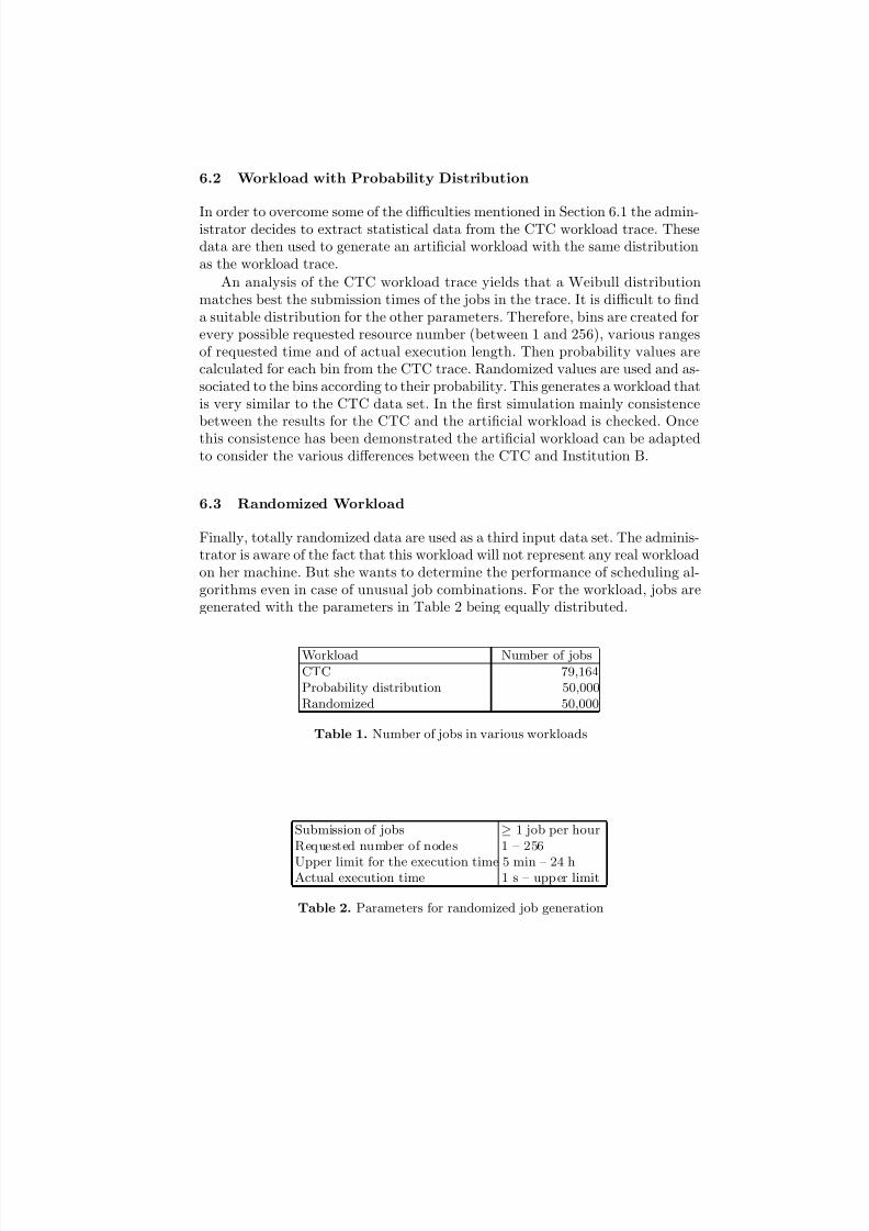
Workload Number of jobsCTC 79,164Probability distribution 50,000Randomized 50,000

Table 1. Number of jobs in various workloads

Submission of jobs ≥ 1 job per hourRequested number of nodes 1 – 256

Upper limit for the execution time 5 min – 24 hActual execution time 1 s – upp er limit

Table 2. Parameters for randomized job generation

7/30/2019 Cei Ipps99


eduler Backf illing E ASY-Backf illing

FCFS

PSRS

SM ART-FFI A

SM ART-NFIW

Gar ey&Gr aham

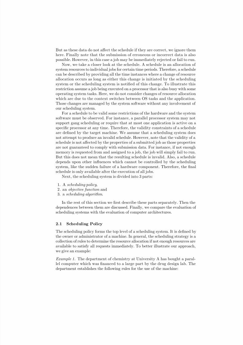
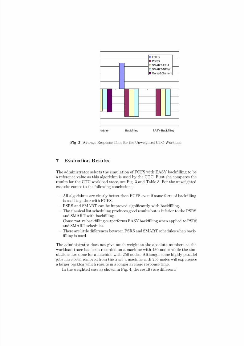
Fig. 3. Average Response Time for the Unweighted CTC-Workload

7 Evaluation Results

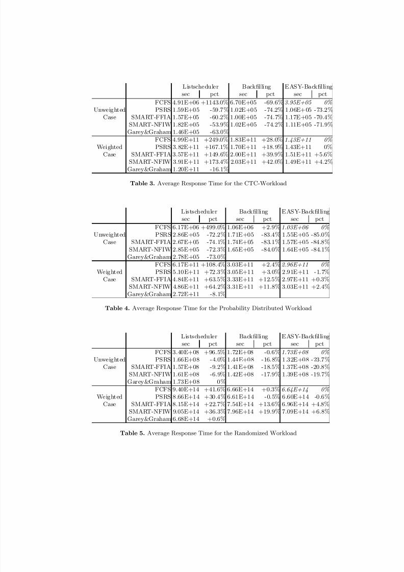
The administrator selects the simulation of FCFS with EASY backfilling to bea reference value as this algorithm is used by the CTC. First she compares the

results for the CTC workload trace, see Fig. 3 and Table 3. For the unweightedcase she comes to the following conclusions:

– All algorithms are clearly better than FCFS even if some form of backfillingis used together with FCFS.

– PSRS and SMART can be improved significantly with backfilling.

– The classical list scheduling produces good results but is inferior to the PSRSand SMART with backfilling.

– Conservative backfilling outperforms EASY backfilling when applied to PSRSand SMART schedules.

– There are little differences between PSRS and SMART schedules when back-filling is used.

The administrator does not give much weight to the absolute numbers as theworkload trace has been recorded on a machine with 430 nodes while the sim-ulations are done for a machine with 256 nodes. Although some highly parallel jobs have been removed from the trace a machine with 256 nodes will experiencea larger backlog which results in a longer average response time.

In the weighted case as shown in Fig. 4, the results are different:

7/30/2019 Cei Ipps99


Listscheduler Backf illing E ASY-Backf illing

FCFS

PSRSSM ART-FFI A

SM ART-NFIW

Gar ey&Gr aham

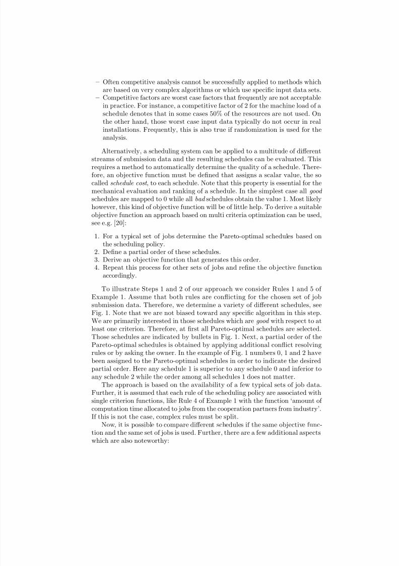
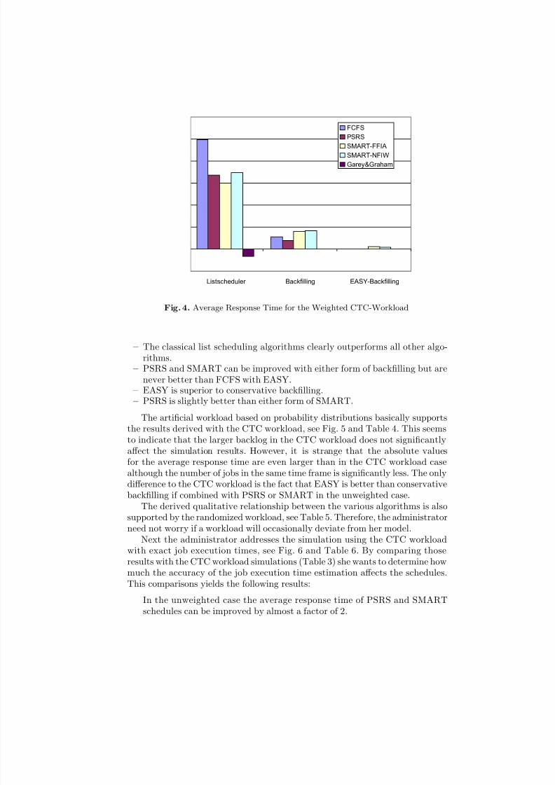
Fig. 4. Average Response Time for the Weighted CTC-Workload

– The classical list scheduling algorithms clearly outperforms all other algo-rithms.

– PSRS and SMART can be improved with either form of backfilling but arenever better than FCFS with EASY.

– EASY is superior to conservative backfilling.– PSRS is slightly better than either form of SMART.

The artificial workload based on probability distributions basically supportsthe results derived with the CTC workload, see Fig. 5 and Table 4. This seemsto indicate that the larger backlog in the CTC workload does not significantlyaffect the simulation results. However, it is strange that the absolute valuesfor the average response time are even larger than in the CTC workload casealthough the number of jobs in the same time frame is significantly less. The onlydifference to the CTC workload is the fact that EASY is better than conservativebackfilling if combined with PSRS or SMART in the unweighted case.

The derived qualitative relationship between the various algorithms is alsosupported by the randomized workload, see Table 5. Therefore, the administratorneed not worry if a workload will occasionally deviate from her model.

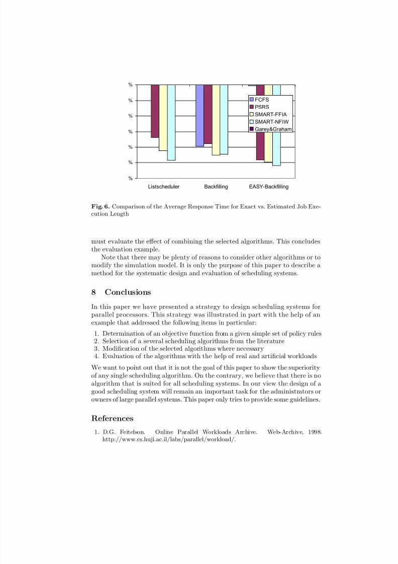
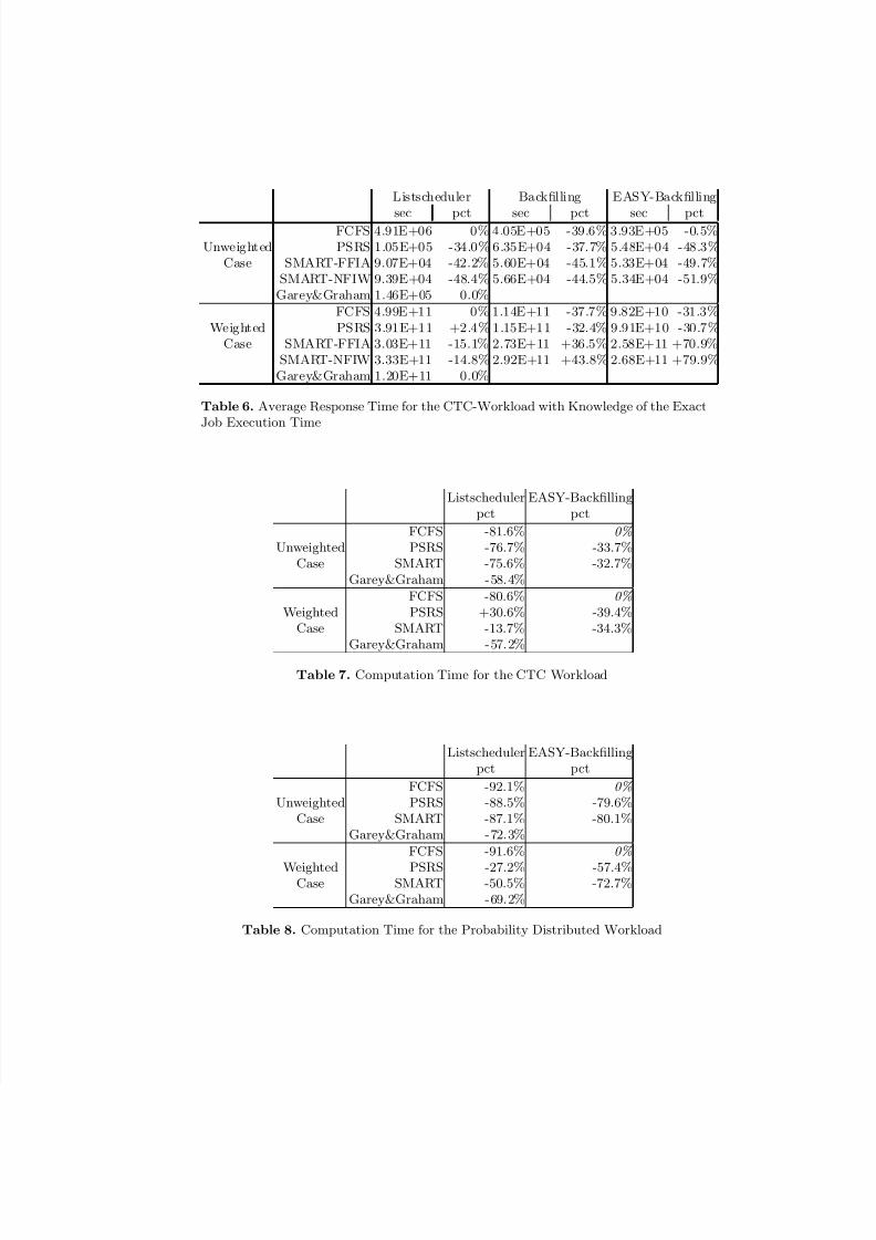
Next the administrator addresses the simulation using the CTC workload

with exact job execution times, see Fig. 6 and Table 6. By comparing thoseresults with the CTC workload simulations (Table 3) she wants to determine howmuch the accuracy of the job execution time estimation affects the schedules.This comparisons yields the following results:

– In the unweighted case the average response time of PSRS and SMARTschedules can be improved by almost a factor of 2.

7/30/2019 Cei Ipps99



FCFS

PSRS

SM ART-FFI A

SM ART-NFIW

Gar ey&Gr aham

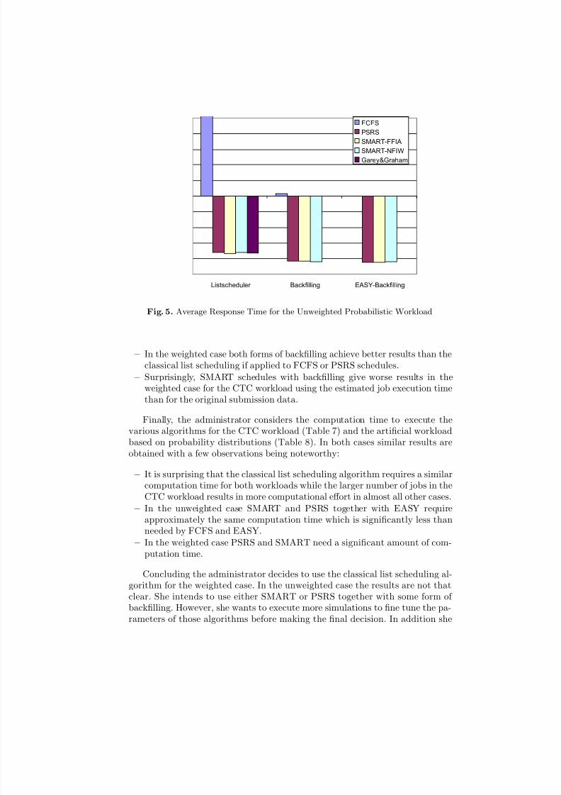
Fig. 5. Average Response Time for the Unweighted Probabilistic Workload

– In the weighted case both forms of backfilling achieve better results than theclassical list scheduling if applied to FCFS or PSRS schedules.

– Surprisingly, SMART schedules with backfilling give worse results in theweighted case for the CTC workload using the estimated job execution timethan for the original submission data.

Finally, the administrator considers the computation time to execute thevarious algorithms for the CTC workload (Table 7) and the artificial workloadbased on probability distributions (Table 8). In both cases similar results areobtained with a few observations being noteworthy:

– It is surprising that the classical list scheduling algorithm requires a similarcomputation time for both workloads while the larger number of jobs in theCTC workload results in more computational effort in almost all other cases.

– In the unweighted case SMART and PSRS together with EASY requireapproximately the same computation time which is significantly less thanneeded by FCFS and EASY.

– In the weighted case PSRS and SMART need a significant amount of com-

putation time.

Concluding the administrator decides to use the classical list scheduling al-gorithm for the weighted case. In the unweighted case the results are not thatclear. She intends to use either SMART or PSRS together with some form of backfilling. However, she wants to execute more simulations to fine tune the pa-rameters of those algorithms before making the final decision. In addition she

7/30/2019 Cei Ipps99



FCFS

PSRS

SM ART-FFI A

SM ART-NFIW

Gar ey&Gr aham

Fig. 6. Comparison of the Average Response Time for Exact vs. Estimated Job Exe-cution Length

must evaluate the effect of combining the selected algorithms. This concludesthe evaluation example.

Note that there may be plenty of reasons to consider other algorithms or tomodify the simulation model. It is only the purpose of this paper to describe amethod for the systematic design and evaluation of scheduling systems.

8 Conclusions

In this paper we have presented a strategy to design scheduling systems forparallel processors. This strategy was illustrated in part with the help of anexample that addressed the following items in particular:

1. Determination of an objective function from a given simple set of policy rules2. Selection of a several scheduling algorithms from the literature3. Modification of the selected algorithms where necessary4. Evaluation of the algorithms with the help of real and artificial workloads

We want to point out that it is not the goal of this paper to show the superiorityof any single scheduling algorithm. On the contrary, we believe that there is noalgorithm that is suited for all scheduling systems. In our view the design of agood scheduling system will remain an important task for the administrators orowners of large parallel systems. This paper only tries to provide some guidelines.

References

1. D.G. Feitelson. Online Parallel Workloads Archive. Web-Archive, 1998.http://www.cs.huji.ac.il/labs/parallel/workload/.

7/30/2019 Cei Ipps99


2. D.G. Feitelson and L. Rudolph. Parallel job scheduling: Issues and approaches.In D.G. Feitelson and L. Rudolph, editors, IPPS’95 Workshop: Job Scheduling

Strategies for Parallel Processing , pages 1–18. Springer–Verlag, Lecture Notes inComputer Science LNCS 949, 1995.3. D.G. Feitelson and L. Rudolph. Metrics and benchmarking for parallel job schedul-

ing. In D.G. Feitelson and L. Rudolph, editors, IPPS’98 Workshop: Job Scheduling Strategies for Parallel Processing , pages 1–24. Springer–Verlag, Lecture Notes inComputer Science LNCS 1459, 1998.

4. D.G. Feitelson and A.M. Weil. Utilization and Predictability in Scheduling theIBM SP2 with Backfilling. In Procedings of IPPS/SPDP 1998 , pages 542–546.IEEE Computer Society, 1998.

5. A. Feldmann, J. Sgall, and S.-H. Teng. Dynamic scheduling on parallel machines.Theoretical Computer Science , 130:49–72, 1994.

6. M. Garey and R.L. Graham. Bounds for multiprocessor scheduling with resourceconstraints. SIAM Journal on Computing , 4(2):187–200, June 1975.

7. M. Garey and D. Johnson. Computers and Intractability: A Guide to the Theory

of NP-Completeness . W. H. Freeman and Company, 1979.8. J.L. Hennessy and D.A. Patterson. Computer Architecture A Quantitative Ap-

proach . Morgan Kaufmann, San Francisco, second edition, 1996.9. S. Hotovy. Workload Evolution on the Cornell Theory Center IBM SP2. In D.G.

Feitelson and L. Rudolph, editors, IPPS’96 Workshop: Job Scheduling Strategies for Parallel Processing , pages 27–40. Springer–Verlag, Lecture Notes in ComputerScience LNCS 1162, 1996.

10. D.A. Lifka. The ANL/IBM SP Scheduling System. In D.G. Feitelson and L.Rudolph, editors, IPPS’95 Workshop: Job Scheduling Strategies for Parallel Pro-cessing , pages 295–303. Springer–Verlag, Lecture Notes in Computer Science LNCS949, 1995.

11. M.E. Rosenkrantz, D.J. Schneider, R. Leibensperger, M. Shore, and J. Zollweg.Requirements of the Cornell Theory Center for Resource Management and Pro-

cess Scheduling. In D.G. Feitelson and L. Rudolph, editors, IPPS’95 Workshop:Job Scheduling Strategies for Parallel Processing , pages 304–318. Springer–Verlag,Lecture Notes in Computer Science LNCS 949, 1995.

12. W. Saphir, L.A. Tanner, and B. Traversat. Job Management Requirements forNAS Parallel Systems and Clusters. In D.G. Feitelson and L. Rudolph, editors,IPPS’95 Workshop: Job Scheduling Strategies for Parallel Processing , pages 319–337. Springer–Verlag, Lecture Notes in Computer Science LNCS 949, 1995.

13. U. Schwiegelshohn. Preemptive weighted completion time scheduling of paral-lel jobs. In Proceedings of the 4th Annual European Symposium on Algorithms (ESA96), pages 39–51. Springer–Verlag Lecture Notes in Computer Science LNCS1136, September 1996.

14. U. Schwiegelshohn, W. Ludwig, J.L. Wolf, J.J. Turek, and P. Yu. Smart SMARTbounds for weighted response time scheduling. SIAM Journal on Computing ,28(1):237–253, January 1999.

15. U. Schwiegelshohn and R. Yahyapour. Improving first-come-first-serve job schedul-ing by gang scheduling. In D.G. Feitelson and L. Rudolph, editors, IPPS’98 Work-shop: Job Scheduling Strategies for Parallel Processing , pages 180–198. Springer–Verlag, Lecture Notes in Computer Science LNCS 1459, 1998.

16. Uwe Schwiegelshohn and Ramin Yahyapour. Analysis of First-Come-First-ServeParallel Job Scheduling. In Proceedings of the 9 th SIAM Symposium on Discrete Algorithms , pages 629–638, January 1998.

7/30/2019 Cei Ipps99


17. Uwe Schwiegelshohn and Ramin Yahyapour. Resource Allocation and Schedulingin Metasystems. In Proceedings of the Distributed Computing and Metacomputing

Workshop at HPCN Europe , April 1999. To appear in Springer–Verlag LectureNotes in Computer Science.18. D. Sleator and R.E. Tarjan. Amortized efficiency of list update and paging rules.

Communications of the ACM , 28:202–208, March 1985.19. W. Smith. Various optimizers for single-stage production. Naval Research Logistics

Quarterly , 3:59–66, 1956.20. R.E. Steuer. Multiple Criteria Optimization, Theory, Computation and Applica-

tion . Wiley, New York, 1986.21. J.J. Turek, U. Schwiegelshohn, J.L. Wolf, and P. Yu. Scheduling parallel tasks to

minimize average response time. In Proceedings of the 5 th SIAM Symposium on Discrete Algorithms , pages 112–121, January 1994.

7/30/2019 Cei Ipps99


Listscheduler Backfilling EASY-Backfillingsec pct sec pct sec pct

FCFS 4.91E+06 +1143.0% 6.70E+05 -69.6% 3.95E+05 0% Unweighted PSRS 1.59E+05 -59.7% 1.02E+05 -74.2% 1.06E+05 -73.2%

Case SMART-FFIA 1.57E+05 -60.2% 1.00E+05 -74.7% 1.17E+05 -70.4%SMART-NFIW 1.82E+05 -53.9% 1.02E+05 -74.2% 1.11E+05 -71.9%

Garey&Graham 1.46E+05 -63.0%FCFS 4.99E+11 +249.0% 1.83E+11 +28.0% 1.43E+11 0%

Weighted PSRS 3.82E+11 +167.1% 1.70E+11 +18.9% 1.43E+11 0%Case SMART-FFIA 3.57E+11 +149.6% 2.00E+11 +39.9% 1.51E+11 +5.6%

SMART-NFIW 3.91E+11 +173.4% 2.03E+11 +42.0% 1.49E+11 +4.2%Garey&Graham 1.20E+11 -16.1%

Table 3. Average Response Time for the CTC-Workload


FCFS 6.17E+06 +499.0% 1.06E+06 +2.9% 1.03E+06 0% Unweighted PSRS 2.86E+05 -72.2% 1.71E+05 -83.4% 1.55E+05 -85.0%


Garey&Graham 2.78E+05 -73.0%FCFS 6.17E+11 +108.4% 3.03E+11 +2.4% 2.96E+11 0%

Weighted PSRS 5.10E+11 +72.3% 3.05E+11 +3.0% 2.91E+11 -1.7%Case SMART-FFIA 4.84E+11 +63.5% 3.33E+11 +12.5% 2.97E+11 +0.3%

SMART-NFIW 4.86E+11 +64.2% 3.31E+11 +11.8% 3.03E+11 +2.4%Garey&Graham 2.72E+11 -8.1%

Table 4. Average Response Time for the Probability Distributed Workload


FCFS 3.40E+08 +96.5% 1.72E+08 -0.6% 1.73E+08 0% Unweighted PSRS 1.66E+08 -4.0% 1.44E+08 -16.8% 1.32E+08 -23.7%


Garey&Graham 1.73E+08 0%FCFS 9.40E+14 +41.6% 6.66E+14 +0.3% 6.64E+14 0%

Weighted PSRS 8.66E+14 +30.4% 6.61E+14 -0.5% 6.60E+14 -0.6%Case SMART-FFIA 8.15E+14 +22.7% 7.54E+14 +13.6% 6.96E+14 +4.8%

SMART-NFIW 9.05E+14 +36.3% 7.96E+14 +19.9% 7.09E+14 +6.8%Garey&Graham 6.68E+14 +0.6%

Table 5. Average Response Time for the Randomized Workload

7/30/2019 Cei Ipps99


Listscheduler Backfilling EASY-Backfilling

sec pct sec pct sec pctFCFS 4.91E+06 0% 4.05E+05 -39.6% 3.93E+05 -0.5%

Unweighted PSRS 1.05E+05 -34.0% 6.35E+04 -37.7% 5.48E+04 -48.3%Case SMART-FFIA 9.07E+04 -42.2% 5.60E+04 -45.1% 5.33E+04 -49.7%

SMART-NFIW 9.39E+04 -48.4% 5.66E+04 -44.5% 5.34E+04 -51.9%Garey&Graham 1.46E+05 0.0%

FCFS 4.99E+11 0% 1.14E+11 -37.7% 9.82E+10 -31.3%Weighted PSRS 3.91E+11 +2.4% 1.15E+11 -32.4% 9.91E+10 -30.7%

Case SMART-FFIA 3.03E+11 -15.1% 2.73E+11 +36.5% 2.58E+11 +70.9%SMART-NFIW 3.33E+11 -14.8% 2.92E+11 +43.8% 2.68E+11 +79.9%

Garey&Graham 1.20E+11 0.0%

Table 6. Average Response Time for the CTC-Workload with Knowledge of the ExactJob Execution Time

Listscheduler EASY-Backfillingpct pct

FCFS -81.6% 0% Unweighted PSRS -76.7% -33.7%

Case SMART -75.6% -32.7%Garey&Graham -58.4%

FCFS -80.6% 0% Weighted PSRS +30.6% -39.4%


Table 7. Computation Time for the CTC Workload

Listscheduler EASY-Backfillingpct pct

FCFS -92.1% 0% Unweighted PSRS -88.5% -79.6%


FCFS -91.6% 0%

Weighted PSRS -27.2% -57.4%Case SMART -50.5% -72.7%

Garey&Graham -69.2%

Table 8. Computation Time for the Probability Distributed Workload

cei ipps99

Documents