brams carlosalbertooliveiradesouzajunior - usp...figure 35 – execution and memory transfer time of...
TRANSCRIPT

UN
IVER
SID
AD
E D
E SÃ
O P
AULO
Inst
ituto
de
Ciên
cias
Mat
emát
icas
e d
e Co
mpu
taçã
o
A hardware/software codesign for the chemical reactivity ofBRAMS
Carlos Alberto Oliveira de Souza JuniorDissertação de Mestrado do Programa de Pós-Graduação em Ciênciasde Computação e Matemática Computacional (PPG-CCMC)


SERVIÇO DE PÓS-GRADUAÇÃO DO ICMC-USP
Data de Depósito:
Assinatura: ______________________
Carlos Alberto Oliveira de Souza Junior
A hardware/software codesign for the chemical reactivity ofBRAMS
Master dissertation submitted to the Instituto deCiências Matemáticas e de Computação – ICMC-USP, in partial fulfillment of the requirements for thedegree of the Master Program in Computer Scienceand Computational Mathematics. FINAL VERSION
Concentration Area: Computer Science andComputational Mathematics
Advisor: Prof. Dr. Eduardo Marques
USP – São CarlosAugust 2017
Ficha catalográfica elaborada pela Biblioteca Prof. Achille Bassi e Seção Técnica de Informática, ICMC/USP,
com os dados fornecidos pelo(a) autor(a)
S684hSouza Junior, Carlos Alberto Oliveira de A hardware/software codesign for the chemicalreactivity of BRAMS / Carlos Alberto Oliveira deSouza Junior; orientador Eduardo Marques. -- SãoCarlos, 2017. 109 p.
Dissertação (Mestrado - Programa de Pós-Graduaçãoem Ciências de Computação e MatemáticaComputacional) -- Instituto de Ciências Matemáticase de Computação, Universidade de São Paulo, 2017.
1. Hardware. 2. FPGA. 3. OpenCL. 4. Codesign. 5.Heterogeneous-computing. I. Marques, Eduardo,orient. II. Título.

Carlos Alberto Oliveira de Souza Junior
Um coprojeto de hardware/software para a reatividadequímica do BRAMS
Dissertação apresentada ao Instituto de CiênciasMatemáticas e de Computação – ICMC-USP,como parte dos requisitos para obtenção do títulode Mestre em Ciências – Ciências de Computação eMatemática Computacional. VERSÃO REVISADA
Área de Concentração: Ciências de Computação eMatemática Computacional
Orientador: Prof. Dr. Eduardo Marques
USP – São CarlosAgosto de 2017


ACKNOWLEDGEMENTS
Firstly, I thank God for being able to fulfill a dream, for giving me health and introducingme wonderful people who supported me to walk through this path. One of them is my advisor,Prof. Eduardo Marques, who is not only wise and patient but also a great friend who has alwaysbeen available to help me to overcome the obstacles in the way.
My sincere gratitude to all my undergraduate professors, in special, I thank ProfessorsEvanise Caldas, Fábio Hernandes, and Mauro Mulati. My friends Lucas Lorenzetti and PauloUrio for sharing the dull and funny moments. To my new friends from LCR (Erinaldo, Mar-cilyanne, and Rafael), who were very welcoming to me. I would also like to thank CNPq fortheir financial support.
Finally, I am deeply thankful to my family. In particular my parents, my grandparentsand my sister Kelly, even with the distance they were always close to me in my thoughts. I loveyou all, and without your support, this dream would not come true.


“I love deadlines. I like the whooshing sound they make as they fly by.”
Douglas Adams


ABSTRACT
OLIVEIRA DE SOUZA JUNIOR, C. A. A hardware/software codesign for the chemicalreactivity of BRAMS . 2017. 109 f. Master dissertation (Master student Program in ComputerScience and Computational Mathematics) – Instituto de Ciências Matemáticas e de Computação(ICMC/USP), São Carlos – SP.
Several critical human activities depend on the weather forecasting. Some of them are transporta-tion, health, work, safety, and agriculture. Such activities require computational solutions forweather forecasting through numerical models. These numerical models must be accurate andallow the computers to process them quickly. In this project, we aim at migrating a small part ofthe software of the weather forecasting model of Brazil, BRAMS — Brazilian developmentson the Regional Atmospheric Modelling System — to a heterogeneous system composed ofXeon (Intel) processors coupled to a reprogrammable circuit (FPGA) via PCIe bus. Accordingto the studies in the literature, the chemical equation from the mass continuity equation isthe most computationally demanding part. This term calculates several linear systems Ax = b.Thus, we implemented such equations in hardware and provided a portable and highly paralleldesign in OpenCL language. The OpenCL framework also allowed us to couple our circuit toBRAMS legacy code in Fortran90. Although the development tools present several problems, thedesigned solution has shown to be viable with the exploration of parallel techniques. However,the performance was below of what we expected.
Keywords: Hardware, FPGA, OpenCL, codesign, heterogeneous-computing.


RESUMO
OLIVEIRA DE SOUZA JUNIOR, C. A. A hardware/software codesign for the chemicalreactivity of BRAMS . 2017. 109 f. Dissertação (Mestrado em Ciências – Ciências de Com-putação e Matemática Computacional) – Instituto de Ciências Matemáticas e de Computação(ICMC/USP), São Carlos – SP.
Várias atividades humanas dependem da previsão do tempo. Algumas delas são transporte, saúde,trabalho, segurança e agricultura. Tais atividades exigem solucões computacionais para previsãodo tempo através de modelos numéricos. Estes modelos numéricos devem ser precisos e ágeispara serem processados no computador.Este projeto visa portar uma pequena parte do softwaredo modelo de previsão de tempo do Brasil, o BRAMS — Brazilian developments on the Regional
Atmospheric Modelling System — para uma arquitetura heterogênea composta por processadoresXeon (Intel) acoplados a um circuito reprogramável em FPGA via barramento PCIe. De acordocom os estudos, o termo da química da equação de continuidade da massa é o termo maiscaro computacionalmente. Este termo calcula várias equações lineares do tipo Ax = b. Destemodo, este trabalho implementou estas equações em hardware, provendo um codigo portável eparalelo na linguagem OpenCL. O framework OpenCL também nos permitiu acoplar o códigolegado do BRAMS em Fortran90 junto com o hardware desenvolvido. Embora as ferramentasde desenvolvimento tenham apresentado vários problemas, a solução implementada mostrou-seviável com a exploração de técnicas de paralelismo. Entretando sua perfomance ficou muitoaquém do desejado.
Palavras-chave: Hardware, FPGA, OpenCL, coprojeto, computação-heterogênea.


LIST OF FIGURES
Figure 1 – Simulation of CCATT-BRAMS system, figure from (LONGO et al., 2013). . 31
Figure 2 – Rosenbrock Method. . . . . . . . . . . . . . . . . . . . . . . . . . . . . . 33
Figure 3 – Jacobi Method algorithm. . . . . . . . . . . . . . . . . . . . . . . . . . . . 37
Figure 4 – Clock rate and power increase of eight generations of Intel microprocessors,figure from (PATTERSON; HENNESSY, 2012). . . . . . . . . . . . . . . . 38
Figure 5 – OpenCL Data Structures – Consider Program as a single data structure; wereplicated it to make the understanding easier. . . . . . . . . . . . . . . . . 40
Figure 6 – An example of how the global IDs, local IDs, and work-group indices are re-lated for a two-dimensional NDRange. For this figure, we have the followingindices: the shaded block has a global ID of (gx,gy) = (6,5), a work-group IDof (wx,wy) = (1,1) plus a local ID of (lx, ly) = (2,1), figure from (MUNSHI,2009). . . . . . . . . . . . . . . . . . . . . . . . . . . . . . . . . . . . . . 41
Figure 7 – Components from OpenCL system on Intel FPGAs, figure from (ALTERA,2013). . . . . . . . . . . . . . . . . . . . . . . . . . . . . . . . . . . . . . 42
Figure 8 – Partitioning of the FPGA. PCIe, DDR3 controller and IPs are every projectof OpenCL, so only the remaining is available for the kernels, figure grantedby André Perina. . . . . . . . . . . . . . . . . . . . . . . . . . . . . . . . . 42
Figure 9 – Implementation of local memory with three M20K blocks, figure from (IN-TEL, 2016a). . . . . . . . . . . . . . . . . . . . . . . . . . . . . . . . . . . 43
Figure 10 – Design flow with OpenCL, figure from (CZAJKOWSKI et al., 2012b). . . . 44
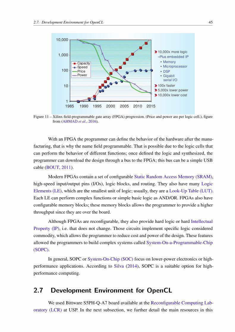
Figure 11 – Xilinx field-programmable gate array (FPGA) progression. (Price and powerare per logic cell.), figure from (AHMAD et al., 2016). . . . . . . . . . . . 45
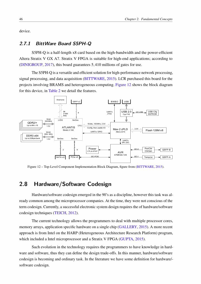
Figure 12 – Top-Level Component Implementation Block Diagram, figure from (BITTWARE,2015). . . . . . . . . . . . . . . . . . . . . . . . . . . . . . . . . . . . . . 46
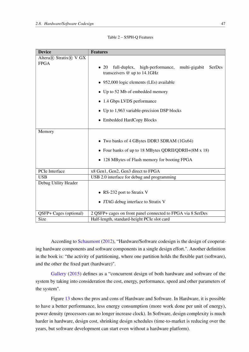
Figure 13 – Driving factors in hardware/software codesign, figure from (SCHAUMONT,2012). . . . . . . . . . . . . . . . . . . . . . . . . . . . . . . . . . . . . . 48
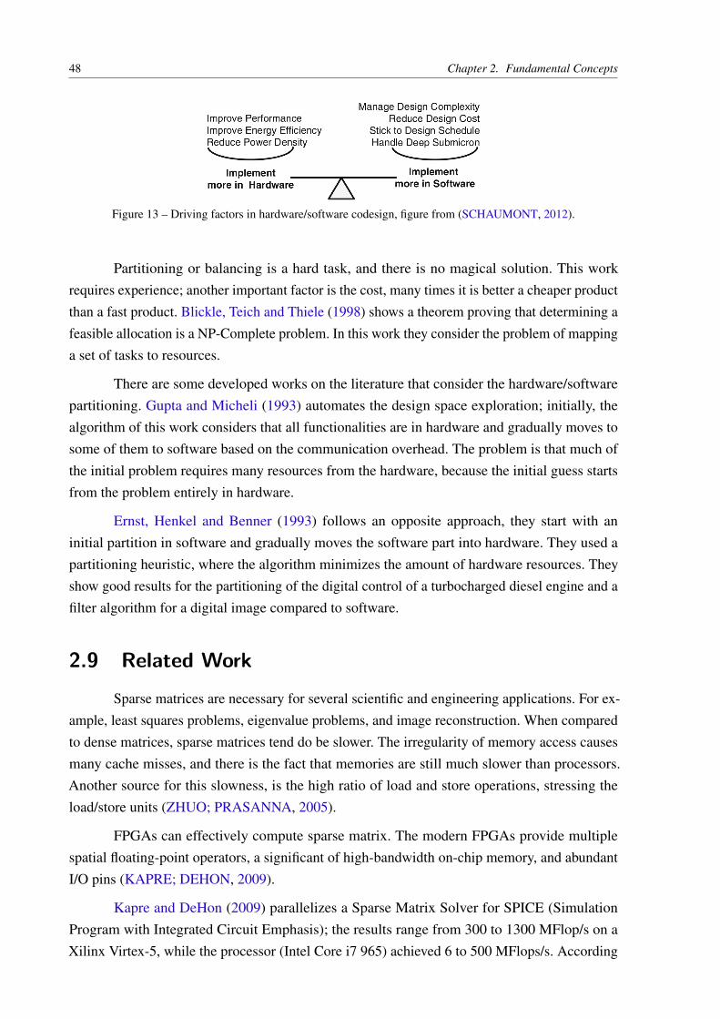
Figure 14 – Speedup compared to CPU versions. The x dimension stands for matrix size,and y dimension speedup in FPGA. . . . . . . . . . . . . . . . . . . . . . . 50
Figure 15 – Generic representation of BRAMS system with a single process. In thisfigure, we present BRAMS over the South America with a single grid, yellowsquare represents Sparse1.3 running for all the points over the grid. . . . . . 56

Figure 16 – Generic representation of BRAMS system with MPI processes. In this figure,we present BRAMS over the South America with a single grid distributedover N processes, each process executes Sparse 1.3 for its set of points of thegrid. The shaded areas are the ghost zones, i.e. the shared data area. . . . . 56
Figure 17 – Generic representation of BRAMS coupled to the Jacobi method in Hardware.In this figure, we present BRAMS over the South America with a single grid,red square represents Jacobi hardware circuit. Such circuit computes all thepoints over the grid. . . . . . . . . . . . . . . . . . . . . . . . . . . . . . . 58
Figure 18 – Schematic of Jacobi method with multiple threads with dense representation. 59
Figure 19 – Each color represents one work-group, each work-group has 47 work-items.According to the verilog, two work-groups are executing at the same time. . 60
Figure 20 – Interoperability of BRAMS and OpenCL. Fortran calls a function from the Chost, which in turn is responsible to manage the device. . . . . . . . . . . . 61
Figure 21 – Schematic of Jacobi method with multiple threads with sparse representation. 63
Figure 22 – Each color represents one work-group, each work-group has one work-item.In this manner, the number of work-items is equal to the number of work-groups. 64
Figure 23 – Schematic of Sparse Jacobi method with single thread. . . . . . . . . . . . . 66
Figure 24 – How pageable and pinned memory data transfer work, based on Harris (2012). 67
Figure 25 – Call Graph for BRAMS with chemical module disabled. . . . . . . . . . . . 70
Figure 26 – Call Graph for BRAMS with chemical module enabled. . . . . . . . . . . . 71
Figure 27 – Each MPI process accesses a copy of the kernel (an FPGA circuit). . . . . . 72
Figure 28 – OpenCL data structures – Program, Device and Memory buffers are sharedamong MPI processes. . . . . . . . . . . . . . . . . . . . . . . . . . . . . . 73
Figure 29 – Pipeline report for Jacobi multi-threaded dense. . . . . . . . . . . . . . . . 74
Figure 30 – CPU communicates with FPGA for every iteration. CPU sends to the FPGAthe initial data, after FPGA processing it, the FPGA returns the result to theCPU, which in turn computes the vector norm and decides if it sends anotherdata or computes another iteration. . . . . . . . . . . . . . . . . . . . . . . 76
Figure 31 – Communication and execution time with Intel FPGA SDK profiling forkernels. Note that there is much more communication than computation. . . 77
Figure 32 – Efficiency of Jacobi multi-threaded dense with Intel FPGA SDK profiling forkernels. The red line points that the global memory reads (line 22) are thebottleneck of the application. . . . . . . . . . . . . . . . . . . . . . . . . . 77
Figure 33 – Statistics of Jacobi multi-threaded dense with Intel FPGA SDK profiling forkernels. . . . . . . . . . . . . . . . . . . . . . . . . . . . . . . . . . . . . . 77
Figure 34 – Efficiency of Jacobi multi-threaded sparse with Intel FPGA SDK profilingfor kernels. Sparse format causes a severe drop of performance when savingthe results back to the global memory. . . . . . . . . . . . . . . . . . . . . 78
Figure 35 – Execution and memory transfer time of Jacobi multi-threaded sparse withIntel FPGA SDK profiling for kernels. Note that transfer time did not improvedue to variable sparsity of the matrices. . . . . . . . . . . . . . . . . . . . . 79
Figure 36 – Statistics of Jacobi multi-threaded sparse with Intel FPGA SDK profiling forkernels. . . . . . . . . . . . . . . . . . . . . . . . . . . . . . . . . . . . . . 79
Figure 37 – Pipeline report for Jacobi single-threaded sparse. . . . . . . . . . . . . . . . 81Figure 38 – Optimum pipeline with II of 1, figure from Intel (2016a). . . . . . . . . . . 82Figure 39 – Matrix-vector pipeline with II of 11, based on Intel (2016a). . . . . . . . . . 82Figure 40 – Pipeline report for Jacobi single-threaded sparse optimized. . . . . . . . . . 83Figure 41 – Efficiency for Jacobi single-threaded sparse. After the modifications, all the
pipelines shows 100% of efficiency and almost zero stall. . . . . . . . . . . 84Figure 42 – Execution and memory transfers time for Jacobi single-threaded sparse. Each
bar in spjacobi_method1 means a complete execution over a matrix. . . . . 85Figure 43 – Statistics for Jacobi single-threaded sparse. . . . . . . . . . . . . . . . . . . 85


LIST OF TABLES
Table 1 – Results from CLOC. . . . . . . . . . . . . . . . . . . . . . . . . . . . . . . 27Table 2 – S5PH-Q Features . . . . . . . . . . . . . . . . . . . . . . . . . . . . . . . . 47Table 4 – Table of comparison among related works . . . . . . . . . . . . . . . . . . . 53Table 6 – Results from Arch 1. . . . . . . . . . . . . . . . . . . . . . . . . . . . . . . 77Table 7 – Timing results from Arch 1. . . . . . . . . . . . . . . . . . . . . . . . . . . 78Table 8 – Results from Arch 2. . . . . . . . . . . . . . . . . . . . . . . . . . . . . . . 80Table 9 – Timing results from Arch 2. . . . . . . . . . . . . . . . . . . . . . . . . . . 80Table 10 – Results from Arch 3. . . . . . . . . . . . . . . . . . . . . . . . . . . . . . . 86Table 11 – Tmining results from Arch 3. . . . . . . . . . . . . . . . . . . . . . . . . . . 86Table 12 – Timing results from Arch 4. . . . . . . . . . . . . . . . . . . . . . . . . . . 87Table 13 – Table of comparison among implementations. . . . . . . . . . . . . . . . . . 87Table 15 – Comparison among architectures . . . . . . . . . . . . . . . . . . . . . . . . 88


19
ACRONYMS
AOCL Altera OpenCL.
API Application Programming Interface.
ARM Advanced RISC Machines.
ATMET ATmospheric, Meteorological, and Environmental Technologies.
BRAMS Brazilian developments on the Regional Atmospheric Modelling System.
CB Carbon Bond.
CBEA Cell Broadband Engine Architecture.
CCATT Coupled Chemistry Aerosol–Tracer Transport.
CDFG Control-Data Flow Graph.
CPTEC Center for Weather Forecasts and Climate Studies.
CPU Central Processing Unit.
CSR Compressed Row Storage.
FINEP Financier of Studies and Projects.
FPGA Field-Programmable Gate Array.
GPU Graphics Processing Unit.
HDF5 Hierarchical Data Format.
HDL Hardware Description Language.
HIPAcc Heterogeneous Image Processing Acceleration Framework.
IAG Institute of Astronomy, Geophysics and Atmospheric Sciences.
II Initiation Interval.
IME Institute of Mathematics and Statistics.

20 Acronyms
INPE National Institute for Space Research.
IP Intellectual Property.
IR Intermediate Representation.
JULES Joint UK Land Environment Simulator.
KPP Kinetic PreProcessor.
LCR Reconfigurable Computing Laboratory.
LE Logic Elements.
LU Lower Upper.
LUT Look-Up Table.
MPI Message Passing Interface.
MPICH Message Passing Interface CHameleon.
MRA Multiresolution Analysis.
NDRange N-Dimensional Range.
NetCDF Network Common Data Form.
OpenCL Open Computing Language.
PBL planetary Boundary Layer.
PCIe Peripheral Component Interconnect Express.
PDE Partial Differential Equations.
RACM Regional Atmospheric Chemistry Mechanism.
RAMS Regional Atmospheric Modeling System.
RELACS Regional Lumped Atmospheric Chemical Scheme.
RTL Register-Transfer Level.
SDK Software Development Kit.
SIMD Single Instruction, Multiple Data.
Acronyms 21
SOC System-On-Chip.
SOPC System-On-a-Programmable-Chip.
SpMV Sparse Matrix-Vector multiplication.
SRAM Static Random Access Memory.
SVD Singular Value Decomposition.
USP University of São Paulo.
CONTENTS
Acronyms . . . . . . . . . . . . . . . . . . . . . . . . . . . . . . . . . . . . . . . 19
1 INTRODUCTION . . . . . . . . . . . . . . . . . . . . . . . . . . . . 251.1 Objective . . . . . . . . . . . . . . . . . . . . . . . . . . . . . . . . . . . 271.2 Motivation . . . . . . . . . . . . . . . . . . . . . . . . . . . . . . . . . . 271.3 Document organization . . . . . . . . . . . . . . . . . . . . . . . . . . . 28
2 FUNDAMENTAL CONCEPTS . . . . . . . . . . . . . . . . . . . . . 292.1 Brazilian developments on the Regional Atmospheric Modelling Sys-
tem – BRAMS . . . . . . . . . . . . . . . . . . . . . . . . . . . . . . . . 292.1.1 CCATT-BRAMS . . . . . . . . . . . . . . . . . . . . . . . . . . . . . . . 302.1.2 Libraries . . . . . . . . . . . . . . . . . . . . . . . . . . . . . . . . . . . . 322.1.3 NetCDF . . . . . . . . . . . . . . . . . . . . . . . . . . . . . . . . . . . . 322.1.4 HDF5 . . . . . . . . . . . . . . . . . . . . . . . . . . . . . . . . . . . . . 342.1.5 Zlib . . . . . . . . . . . . . . . . . . . . . . . . . . . . . . . . . . . . . . . 342.1.6 Szip . . . . . . . . . . . . . . . . . . . . . . . . . . . . . . . . . . . . . . 342.1.7 Mpich . . . . . . . . . . . . . . . . . . . . . . . . . . . . . . . . . . . . . 342.1.7.1 MPI . . . . . . . . . . . . . . . . . . . . . . . . . . . . . . . . . . . . . . . 352.2 Linear Equation . . . . . . . . . . . . . . . . . . . . . . . . . . . . . . . 352.3 Linear Solver . . . . . . . . . . . . . . . . . . . . . . . . . . . . . . . . . 362.3.1 Direct Method - LU . . . . . . . . . . . . . . . . . . . . . . . . . . . . . 362.3.2 Iterative Method - Jacobi . . . . . . . . . . . . . . . . . . . . . . . . . 362.4 OpenCL . . . . . . . . . . . . . . . . . . . . . . . . . . . . . . . . . . . . 372.4.1 Data structures for OpenCL . . . . . . . . . . . . . . . . . . . . . . . . 382.4.2 Data Parallelism . . . . . . . . . . . . . . . . . . . . . . . . . . . . . . . 392.4.3 Task Parallelism . . . . . . . . . . . . . . . . . . . . . . . . . . . . . . . 402.5 Intel FPGA SDK for OpenCL . . . . . . . . . . . . . . . . . . . . . . . 412.6 FPGA . . . . . . . . . . . . . . . . . . . . . . . . . . . . . . . . . . . . . 442.7 Development Environment for OpenCL . . . . . . . . . . . . . . . . . 452.7.1 BittWare Board S5PH-Q . . . . . . . . . . . . . . . . . . . . . . . . . . 462.8 Hardware/Software Codesign . . . . . . . . . . . . . . . . . . . . . . . 462.9 Related Work . . . . . . . . . . . . . . . . . . . . . . . . . . . . . . . . 48

Contents 23
3 DEVELOPMENT OF THE CODESIGN FOR THE CHEMICAL RE-ACTIVITY OF BRAMS . . . . . . . . . . . . . . . . . . . . . . . . . 55
3.1 CCATT–BRAMS software . . . . . . . . . . . . . . . . . . . . . . . . . 553.1.1 Interoperability with Sparse1.3a . . . . . . . . . . . . . . . . . . . . . 573.2 CCATT–BRAMS Codesign . . . . . . . . . . . . . . . . . . . . . . . . 573.2.1 Jacobi Multi-threaded Dense . . . . . . . . . . . . . . . . . . . . . . . 573.2.2 Interoperability with Jacobi Multi-Threaded Dense . . . . . . . . . . 603.2.3 Jacobi Multi-threaded Sparse . . . . . . . . . . . . . . . . . . . . . . . 623.2.4 Interoperability with Jacobi Multi-Threaded Sparse . . . . . . . . . . 633.2.5 Jacobi Single-threaded Sparse . . . . . . . . . . . . . . . . . . . . . . . 643.2.6 Interoperability with Jacobi Single-threaded Sparse . . . . . . . . . . 67
4 RESULTS . . . . . . . . . . . . . . . . . . . . . . . . . . . . . . . . . 694.1 Result analysis . . . . . . . . . . . . . . . . . . . . . . . . . . . . . . . . 694.2 Experiments . . . . . . . . . . . . . . . . . . . . . . . . . . . . . . . . . 704.3 Results from Jacobi Multi-threaded Dense . . . . . . . . . . . . . . . 734.4 Results from Jacobi Multi-threaded Sparse . . . . . . . . . . . . . . . 784.5 Results from Jacobi Single-threaded Sparse . . . . . . . . . . . . . . 804.6 Results from Jacobi Single-threaded Dense . . . . . . . . . . . . . . . 864.7 Results from Sparse1.3a . . . . . . . . . . . . . . . . . . . . . . . . . . 87
5 CONCLUSION . . . . . . . . . . . . . . . . . . . . . . . . . . . . . . 895.1 Limitations . . . . . . . . . . . . . . . . . . . . . . . . . . . . . . . . . . 895.2 Future Work . . . . . . . . . . . . . . . . . . . . . . . . . . . . . . . . . 90
BIBLIOGRAPHY . . . . . . . . . . . . . . . . . . . . . . . . . . . . . . . . . . . 91
APPENDIX . . . . . . . . . . . . . . . . . . . . . . . . . . . . . . . . . . . . . . 101
APPENDIX . . . . . . . . . . . . . . . . . . . . . . . . . . . . . . . . . . . . . . 103
APPENDIX A INSTALLATION . . . . . . . . . . . . . . . . . . . . . 103
APPENDIX B OBSERVING THE RESULTS . . . . . . . . . . . . . . 107
ANNEX A USEFUL LINKS . . . . . . . . . . . . . . . . . . . . . . . . 109


25
CHAPTER
1INTRODUCTION
Weather forecasting is the utilization of science and technology to predict the stateof the atmosphere at a provided location. The predictions require quantitative data from thecurrent situation of the atmosphere at a given place, and scientific understanding of atmosphericprocesses to predict how the atmosphere will change (HENKEL, 2015).
According to Society (2015) the meteorological profession is responsible for two crucialservices: weather forecasts and warnings. The government and industry use forecasts to protectlife and property and to improve the efficiency of operations.
Several critical human activities depend on the weather forecasting. Some of them aretransportation, health, work, and safety. Imagine an air travel where passengers do not knowwhat are the risks ahead; a forest fire where firefighters have no clue where the fire will move(LABORATORY, 2015).
Forecasts based on temperature and precipitation are important to agriculture and so thetraders of commodity markets. Weather forecasting is also critical to estimate the crop-diseasespread (WARNER, 2010). Trying to predict the weather is not a new science.
Ancient civilizations started to forecast the weather at the very early ages. They usedastronomical and meteorological events to keep track of seasonal changes in the weather. By theyear 650 B.C., Babylonians tried to predict weather (short-term) through clouds patterns andoptical phenomena, such as halos (GRAHAM; PARKINSON; CHAHINE, 2002).
By the end of Renaissance period, it had become clear to philosophers that forecastingbased only on observations and assumptions was not an adequate method. They needed toimprove their understanding of the atmosphere — the development of new tools was necessaryto measure properties of the atmosphere, such as moisture, temperature, and pressure. The firsttool dates back to 14th century, the hygrometer.
On the 16th century, Galileo Galilei invented the thermometer. Later in the 17th century,
26 Chapter 1. Introduction
Evangelista Torricelli created the barometer. Other tools came later on recently centuries (forexample radiosonde and weather satellite). These instruments allowed us to create weatherobservation stations and the dissemination of them around the globe. Besides the tools, it wasalso necessary a better understanding of the atmosphere.
In the 19th century, the development of thermodynamics allowed meteorologists to setthe fundamental physical principles that govern the flow of the atmosphere (LYNCH, 2008). In1890, Cleveland Abbe acknowledged that meteorology is the application of hydrodynamics andthermodynamics to the atmosphere (WILLIS; HOOKE, 2006).
In 1904, Vilhelm Bjerknes published a paper in german (The Problem of WeatherForecasting from the Standpoint of Mechanics and Physics). In this paper, he introduces the hydro-and thermodynamics into meteorology. Vilhelm included the second law of thermodynamics inhis set of equations; this error was corrected by Lewis Fry Richardson (GRØNØS, 2005). Thelatter made an estimate method for solving numerical equations — According to Richardson, itwould be required 64 thousand people to predict the weather in time. It is clear that predictingthe weather was impossible before computational era (LYNCH, 2008).
Predicting the weather became possible in the 20th century, with Von Neumann’s ENIAC.Charney realized that could overcome Richardson’s methods impracticability with new com-puters, and a revised set of equations where scientists could solve complex equations throughnumerical methods. In April 1950, Charney’s research group succeed to predict the weather for24 hours in the North America.
With the computer availability increasing in the 20th century, universities started offeringcourses on atmospheric modeling. At the time, people shared their time as both modelers anddevelopers; the generated code had many errors, so it was necessary more human effort to correctit. The development in the field allowed the modelers to have available, for free, well-testedcommunity, global and limited-area models, and access to full documentation, regular tutorials,and technical support (WARNER, 2010).
Last century was responsible for many scientific advances that allowed us to predict theweather phenomena. This prediction uses numerical models; we can classify such models accord-ing to their domain operation: Global (the entire Earth planet) and regional (e.g. Country, State,and City). The global models cannot represent accurately the regional weather phenomena dueto limited computing power. On the other hand, regional models are more accurate (OSTHOFFet al., 2012; LABORATORY, 2015). In this project, we are using Brazilian developments on theRegional Atmospheric Modelling System (BRAMS)1, a Brazilian regional model.
Currently, BRAMS is the largest high-performance application in Brazil according toPanetta (2015). We used a PERL script to count the lines of BRAMS, with CLOC2 we discovered
1 http://brams.cptec.inpe.br/2 http://cloc.sourceforge.net/

1.1. Objective 27
that BRAMS has over 400 thousands lines of code in Fortran. We can see the results in Table 1.Since the application is huge, we used some tools available on the Internet to detect bottlenecksand generate graphical data, they are Gprof, and Gprof2dot, respectively.
Table 1 – Results from CLOC.
Language Files Blank Comment Code
Fortran 90 748 67905 126111 454676
C 14 2154 5102 6062
Bourne Shell 4 694 857 5081
C/C++ Header 39 390 1129 1496
make 18 186 173 891
Sum 823 71329 133372 468206
1.1 ObjectiveThe main objective of this work is to show that is viable to migrate segments of code
of BRAMS to a heterogeneous architecture, particularly hardware platforms that use XeonIntel processor coupled to a programmable circuit (FPGA) via PCIe. Thus, we can providea hardware/software solution for a snippet of BRAMS that will be functionally integrated toBRAMS.
According to the studies in the literature, the chemical equation from the mass continuityequation is the most computationally demanding part. This term calculates several linear systemsAx = b. Thus, we implemented such equations in hardware and provided a portable and highlyparallel design in OpenCL language. The OpenCL framework also allowed us to couple ourcircuit to BRAMS legacy code in Fortran90. Although the development tools present severalproblems, the designed solution has shown to be viable with the exploration of parallel techniques.However, the performance was below of what we expected.
1.2 MotivationThe weather prediction is considered a super application or a supercomputing application.
They demand high computing power with increasing inclination for growth (KIRK; WEN-MEI,2012).
In the last 20 years, processors have increased in 1000 times their performance. Increasingthe performance of current processors require changes in the architecture. Due to energy limits, itis not viable to boost the frequency on current state-of-art processors. This limitation has forced
28 Chapter 1. Introduction
designers to use large-scale parallelism, heterogeneous cores, and accelerators for demandingapplications (BORKAR; CHIEN, 2011).
The applications will depend on customized accelerators, especially in hardware, to gainperformance. In many cases, the acceleration also improves computational efficiency regardingthe energy consumption compared to a solution based on software (CONG; ZOU, 2009).
Accelerators are special-purpose processors used to accelerate CPU-bound applications.The development of them is usually in Graphics Processing Unit (GPU) or Field-ProgrammableGate Array (FPGA); both can achieve substantial performance for certain workloads whencompared to Central Processing Unit (CPU). FPGAs are highly customizable and, in general,offer the best performance (CHE et al., 2008).
1.3 Document organizationIn Chapter 2, we present the fundamental concepts for this project and the literature
review. In Chapter 3, we describe our three architectures for Jacobi method. We also describehow we managed the interoperability with CPU for each architecture. In Chapter 4, we presentthe profiling that supports that the chem term is the most expensive in the mass continuityequation. Then we show the results for each architecture and its problems. Lastly, we compareour hardware solution with the current software solution in BRAMS. In Chapter 5, we concludeour project and present the main limitations and future work. In Appendix A, we depict theinstallation of BRAMS. In Appendix B, we show how to visualize the results from BRAMS. InAnnex A, there are useful links to libraries, additional software, and BRAMS source code.

29
CHAPTER
2FUNDAMENTAL CONCEPTS
2.1 Brazilian developments on the Regional AtmosphericModelling System – BRAMS
BRAMS is an project originally developed by ATmospheric, Meteorological, and Envi-ronmental Technologies (ATMET), IME/USP (Institute of Mathematics and Statistics/Universityof São Paulo), IAG/USP (Institute of Astronomy, Geophysics and Atmospheric Sciences) andCPTEC/INPE (Center for Weather Forecasts and Climate Studies/National Institute for SpaceResearch), and funded by Financier of Studies and Projects (FINEP) (Brazilian Funding Agency)(INPE/CPTEC, 2015).
They aimed at producing an adapted version of Regional Atmospheric Modeling System(RAMS) for the tropics (FREITAS et al., 2009), which provided a single model to BrazilianRegional Weather Centers. One of the purposes of BRAMS/RAMs is to simulate atmosphericcirculations through a numerical prediction model. The simulation can range from hemisphericscales down to large eddy simulations (LES) of the planetary boundary layer (LONGO et al.,2013).
Since version 4.2, the CPTEC/INPE team is responsible for the entire software develop-ment. BRAMS uses the cathedral model. Software built in a cathedral model must provide thesource-code every release, and only the software developers can access the source-code betweenreleases (RAYMOND, 2001). The software license is under CC-GNU-GPL, and some parts mayreceive other restricted licenses.
Three main models represent BRAMS. The tracer transport model, chemical model(Coupled Chemistry Aerosol–Tracer Transport (CCATT)) and a surface model. BRAMS in-corporate the tracer transport model and chemical model, and Joint UK Land EnvironmentSimulator (JULES) is the name of the surface model. In this dissertation, we focus on CCATT,more specifically the numerical solution of the chemical reactivity.

30 Chapter 2. Fundamental Concepts
2.1.1 CCATT-BRAMS
CATT-BRAMS is a Eulerian atmospheric chemistry transport model fully coupled toBRAMS. Its design allows us to study transport processes associated with the emission of tracersand aerosols (FREITAS et al., 2010). CATT-BRAMS solves the mass continuity equation fortracers; we present it in Equation (2.1).
∂ s∂ t
=
(∂ s∂ t
)adv
+
(∂ s∂ t
)PBL di f f
+
(∂ s∂ t
)deep conv
+(∂ s∂ t
)shallow conv
+
(∂ s∂ t
)chem
+W +R+Q(2.1)
“Where s is the grid box mean tracer mixing ratio” (LONGO et al., 2013); a prognostic variable,this variable is governed by the prognostic equation, which means that involve derivatives(RANDALL, 2013). “The term adv represents the 3-D resolved transport (advection by the meanwind); and the terms PBL diff, deep conv, and shallow conv stand for the sub-grid scale turbulencein the Planetary Boundary Layer (PBL), and deep and shallow convection, respectively”.
Advection and convection stand for the transfer of energy generated by the movement ofparticles of liquid like water in the atmosphere. Advection transfer horizontally, and convectiontransfer energy vertically (ACKERMAN; ACKERMAN; KNOX, 2013). Deep convection isthe thermally driven turbulent mixing that lifts the air from the lower to the upper atmosphere.“Shallow convection: thermally driven turbulent mixing, where vertical lifting is capped below500hPa” (DAVISON, 1999; VAUGHAN, 2009).
“The chem term refers simply to the passive tracers’ lifetime, the W is the term for wetremoval applied only to aerosols, and R is the term for the dry deposition applied to both gassesand aerosol particles” (LONGO et al., 2013).
CATT-BRAMS evolved to CCATT-BRAMS (Chemistry CATT-BRAMS). This newmodel includes a gas phase chemical module, which solves chem term in Equation (2.1). Weshow this module in Equation (2.2).
(∂ρk∂ t
)chem
=
(dρkdt
)= Pk(ρ)−Lk(ρ), (2.2)
Where ρ stands for the number density for each of the N species, and Pk and Lk are the netproduction and loss of species k, respectively. P and L terms include photochemistry, gas phase,and aqueous chemistry. The solution of this equation is the most expensive term of Equation (2.1).
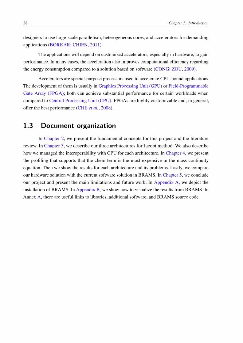
The development of CCATT required advanced numerical tools to provide a flexiblemulti-purpose model, i.e. the model can run for both operational forecasts and research simula-tions. Figure 1 illustrates the simulation of CCATT-BRAMS system. The illustration representsthe primary sub-grid scale processes involved in the trace gas and aerosol distributions.
2.1. Brazilian developments on the Regional Atmospheric Modelling System – BRAMS 31
Figure 1 – Simulation of CCATT-BRAMS system, figure from (LONGO et al., 2013).
Moreover, the model system allows the user to provide any chemical mechanism. Cur-rently, there are three widely used chemistry mechanisms; they are as follows: Regional Atmo-spheric Chemistry Mechanism (RACM) with 77 species (STOCKWELL et al., 1997), CarbonBond (CB) with 36 species (YARWOOD et al., 2005), and the Regional Lumped AtmosphericChemical Scheme (RELACS) with 37 species (CRASSIER et al., 2000).
Scientific projects frequently use RACM mechanism due to its number of species itcovers; RELACS is a reduced version of RACM. CPTEC uses RELACS for operational airquality prediction. According to Gácita (2011), RELACS can replicate RACM results reasonablywell.
To solve the Equation (2.2) with k species Longo et al. (2013) uses Rosenbrock method(WANNER; HAIRER, 1991; VERWER et al., 1999) to change from nonlinear differentialequation system to a linear algebraic increment in terms of Ki. In this method, the integrationstep is adjusted as a function of the calculated error (FERNANDES, 2014).
The solution of this linear algebraic increment, which corresponds to P and L, is inEquation (2.3).
ρ(t0 + τ) = ρ(t0)+s
∑i=1
biKi, (2.3)
Where t0 stands for initial concentration, τ is the timestep. The product sum approximates theintegral, where i is the Rosenbrock stage. Each timestep and stage require the update of Ki

32 Chapter 2. Fundamental Concepts
increment according to the linear system in Equation (2.4a).
Ki = τF(ρi)+ τJ(ρ(t0)).i
∑j=1
γi jK j
ρi = ρ(t0)+i−1
∑j=1
ai jK j
F(ρi) = P(ρi)−L(ρi),
(2.4a)
(2.4b)
(2.4c)
Where ai j and γi j are constants that depend on s, ρi stands for the intermediate solution used forrecalculating the net production on stage i given by the term F(ρi), and J is the Jacobian matrixof the net production at time t0. Solving the Equation (2.5) is the most computing intensive.
Ax = b (2.5)
Where A is a N ×N matrix, N is the number of species. The vector x is the solution, and b isthe right-hand side or vector of the independent terms. BRAMS solves the Equation (2.4b) byusing Sparse1.3a (KUNDERT; SANGIOVANNI-VINCENTELLI, 1988). In Figure 2 we showthe pseudo-algorithm for the Rosenbrock method with Sparse1.3a to solve each stage.
CCATT-BRAMS runs operationally at CPTEC/INPE since 2003; it covers the entireSouth America with a spatial resolution of 25 km. It is possible to predict the emission of Gasesand Aerosols in real time1, as well as meteorological variables2 (MOREIRA et al., 2013).
2.1.2 Libraries
In this subsection, we will briefly explain each library necessary for BRAMS.
2.1.3 NetCDF
According to Rew (2015) Network Common Data Form (NetCDF) “is a set of interfacesfor array-oriented data access and a freely-distributed collection of data access libraries for C,Fortran, C++, Java, and other languages. The netCDF libraries support a machine-independentformat for representing scientific data. Together, the interfaces, libraries, and format support thecreation, access, and sharing of scientific data".
This library creates an abstraction level for machine-dependent data representation.Such abstraction allows the application to share those files across the networks on differentworkstations. Programs with NetCDF interface can read and write data without the restriction ofmachine-dependent binary data files (REW; DAVIS, 1990).
1 http://meioambiente.cptec.inpe.br/2 http://previsaonumerica.cptec.inpe.br/golMapWeb/DadosPages?id=CCattBrams

2.1. Brazilian developments on the Regional Atmospheric Modelling System – BRAMS 33
Input: Sparse1.3 data structure1 begin2 foreach block do3 foreach grad_point do4 Read variables from BRAMS;5 Update photolysis rate;
6 Compute initial kinetic reactions;7 while Timestep < threshold do8 Compute Jacobian of the matrix of concentrations;9 Compute Equation (2.2);
10 foreach chemical_specie do11 foreach grad_point do12 Update F (ρ) on the data structure;
13 while error > tolerance do14 foreach chemical_specie do15 foreach grad_point do16 Update matrix A;
17 Update bi;18 foreach grad_point do19 Compute 1st Rosenbrock method;
20 Update bi;21 foreach grad_point do22 Compute 2nd Rosenbrock method;
23 Update matrix of concentrations ρ;24 Update production term F (ρ);25 Update bi;26 foreach grad_point do27 Compute 3rd Rosenbrock method;
28 Update matrix of concentrations ρ;29 Update production term F (ρ);30 Update bi;31 foreach grad_point do32 Compute 4th Rosenbrock method;
33 Update matrix of concentrations ρ;34 Compute error and rounding;35 if tolerance - rounding > 1.0 then36 Accept solution;
37 else38 Compute the new integration step;
39 Update the integration step;
40 Update variables from BRAMS;
Algorithm: Rosenbrock Method
Figure 2 – Rosenbrock Method.

34 Chapter 2. Fundamental Concepts
The NetCDF software was developed by Glenn Davis, Russ Rew, Ed Hartnett, JohnCaron, Dennis Heimbigner, Steve Emmerson, Harvey Davies, and Ward Fisher at the UnidataProgram Center in Boulder, Colorado, and many users also contributed to software development.
2.1.4 HDF5
With the Hierarchical Data Format (HDF5) technology suite is possible to organize, store,discover, access, analyze, share, and preserve diverse, complex data in heterogeneous computingand storage environments (GROUP, 2011).
HDF5 supports all types of digital data from any origin or size. This suite is useful fordata collected from satellites, nuclear testing models, high-resolution MRI brain scans. Besidesthe data, HDF5 files also contain the metadata necessary for efficient data sharing, processing,visualization, and archiving.
According to Fazenda et al. (2012), BRAMS uses HDF5 to overcome data writing phasethat was preventing scalability of BRAMS to 9,600 cores; in this work, they used a techniquecalled disk-direct. Such technique was essential to perform I/O collective operations; theseoperations interpolate the sub-domains in a single file in an external memory.
2.1.5 Zlib
Zlib is a library for lossless data-compression for use virtually on any computer hardwareand operating system. The data format from zlib is portable across platforms. Jean-loup Gaillyand Mark Adler are responsible for Zlib creation (GAILLY; ADLER, 2015).
2.1.6 Szip
Szip is a data compressor for data from the sphere. For energy compression, it uses aHaar wavelet transform on the sphere. This transformation reduces the entropy of the data. Afterthis transformation, it encodes with Huffman and run-length. Both compression algorithms arelossless and lossy (MCEWEN; EYERS, 2011).
2.1.7 Mpich
Message Passing Interface CHameleon (MPICH) is a portable implementation of the Mes-sage Passing Interface (MPI). Of the goals of MPICH is to provide efficient MPI implementationfor different computation and communication platforms (MPICH, 2015).
MPICH is open source. It works on several platforms, including Linux (on IA32 andx86-64), Mac OS/X (PowerPC and Intel), Solaris (32- and 64-bit), and Windows.

2.2. Linear Equation 35
2.1.7.1 MPI
Programming and debugging for parallel algorithms are much more complicated thanprogramming for sequential algorithms. There are several models of parallel programming; theyare as follows (NIELSEN, 2016):
∙ Vector supercomputers, which relies on Single Instruction, Multiple Data (SIMD);
∙ Multi-core machines with shared memory, which uses multi-threading;
∙ Clusters of computer machines with distributed memory.
The latter can include the first and the second parallel programming; this is the parallelprogramming paradigm suitable for MPI. Each node can execute a program using its localmemory, and cooperation among nodes depends on sending and receiving messages (GROPP et
al., 2014).
Message Passing Interface is an Application Programming Interface (API). This APIhides the fine details of implementation from the programmer, and it also provides portabilityand efficiency with a wide acceptance from academy and industry. This API works with mostcommon sequential languages, i.e. C, C++, Java, Fortran and so on (KARNIADAKIS; KIRBY,2003).
2.2 Linear EquationAccording to Anton and Rorres (2013), Larson (2016), a linear equation in n variables
x1,x2,x3 . . .xn = b can be represented in the form of the Equation (2.6).
a1x1 +a2x2 + . . .+anxn = b (2.6)
A system with m equations in n variables is called linear system. In Equation (2.7) wepresent a general linear system of this form.
a11x1 +a12x2 + . . .+a1nxn = b1
a21x1 +a22x2 + . . .+a2nxn = b2
......
am1x1 +am2x2 + . . .+amnxn = bm
(2.7)
A solution whose x1,x2,x3 . . .xn satisfies every equation is called consistent. Otherwise,it is inconsistent.

36 Chapter 2. Fundamental Concepts
2.3 Linear SolverAccording to Golub and Loan (2013) and Peng (2013), there are two fundamental
categories to solve linear systems: direct and iterative methods.
2.3.1 Direct Method - LU
In theory, direct methods return the exact solution after a finite number of operations; inpractice, this is not possible due to rounding errors. Lower Upper (LU) decomposition, Cholesky,Gaussian elimination are the main algorithms from this category.
Currently, BRAMS uses LU decomposition to solve the linear systems. Such methodis computationally expensive, since LU decomposition requires O(n3) and solving throughbackward and forward substitution requires O(n2) (BINDEL; GOODMAN, 2006). The libraryresponsible for decomposition and substitution is Sparse1.3a.
Sparse 1.3 is a package of subroutines in C for solving large sparse systems of linearequations. This library manages the necessary memory for the sparse matrix by using linked-listrepresentation; it also offers an interface for Fortran, which turned the integration to BRAMSmuch simpler. Its original purpose was for use in circuit simulators; it is also able to handle nodeand modified-node admittance matrices (KUNDERT; SANGIOVANNI-VINCENTELLI, 1988).
2.3.2 Iterative Method - Jacobi
Regarding the iterative solvers, they offer an approximate solution after an infiniteconvergence process. Those algorithms convergences to x = A−1b. Although simple, Jacobi hasa highly parallel nature. Equation (2.8) shows an instance of Jacobi for a 3×3 matrix (GOLUB;LOAN, 2013; MORRIS; PRASANNA, 2005).
x1 = (b1 −a12x2 −a13x3)/a11,
x2 = (b2 −a21x1 −a23x3)/a22,
x3 = (b3 −a31x1 −a32x2)/a33.
(2.8)
The current solution of this method requires the solution of the previous iteration. Inthe first iteration, it is common to suppose that all variables from the linear system are zero. InEquation (2.9) we show this computation, assume that x(k−1) is the previous solution and x(k) isthe new approximation; from this equation, it is clear that the main diagonal is nonzero.
x(k)1 = (b1 −a12x(k−1)2 −a13x(k−1)
3 )/a11,
x(k)2 = (b2 −a21x(k−1)1 −a23x(k−1)
3 )/a22,
x(k)3 = (b3 −a31x(k−1)1 −a32x(k−1)
2 )/a33.
(2.9)

2.4. OpenCL 37
The general algorithm for Jacobi is in Figure 3.
Input: Matrix A, Vector x, Vector bOutput: Vector x
1 begin2 for i < n do3 for j < n do4 if i ≠ j then5 sum= sum+Ai j ×xk−1
j ;
6 xki =(bi−sum)/ aii;
7 return x
Algorithm: Jacobi Method
Figure 3 – Jacobi Method algorithm.
From this algorithm, it is possible to infer a parallel computation of each row i sincethere is no dependence among rows. Iterative methods require stopping criteria that can identifywhen the error is small enough; this is essential for time execution as well. In our algorithm weused vector norm as the stopping criteria, we present vector norm in Equation (2.10).
‖x‖p =(∣∣xp
1
∣∣+ . . .+ |xpn |)1/p (2.10)
In this case, we consider p = 2, which is the Euclidian norm (standard vector length). Aswe want to measure the Euclidian distance between two vectors, the current solution and theprevious solution, we use Equation (2.11). This distance must be close to zero, which means thatthe solution converged.
ξabs = ‖x(k)− x(k−1)‖ (2.11)
We implemented Figure 3 and the stopping criteria in Equation (2.11) in hardware usingOpen Computing Language (OpenCL). Intel FPGA SDK (Software Development Kit) allowedus to implement hardware in FPGA by using the OpenCL framework.
2.4 OpenCLUntil 2004, programmers could improve software time execution by just changing to a
processor with a higher clock frequency. When Intel CPUs reached 3.6Ghz (TSUCHIYAMA et
al., 2012; MUNSHI et al., 2011), cooling commodity microprocessors became impractical; inFigure 4, we show the increase of clock rate and power (PATTERSON; HENNESSY, 2012).
From this point on, it was evident to the vendor that increasing clock rate was notpossible anymore. That forced the vendors to invest their money and efforts to change the

38 Chapter 2. Fundamental Concepts
2667
12.5 16
2000
20066
25
3600
75.395
29.110.14.94.13.3
103
1
10
100
1000
10000
8028
6(1
982)
8038
6(1
985)
8048
6(1
989)
Pent
ium
(199
3)
Pent
ium
Pro
(199
7)
Pent
ium
4W
illam
ette
(200
1)Pe
ntiu
m 4
Pres
cott
(200
4)C
ore
2Ke
ntsf
ield
(200
7)
Clo
ck R
ate
(MH
z)
0
20
40
60
80
100
120
Pow
er (W
atts
)
Clock Rate
Power
Figure 4 – Clock rate and power increase of eight generations of Intel microprocessors, figure from (PATTERSON;HENNESSY, 2012).
design of the processors; from 2006 until now, all desktop and server companies decided to shipmultiprocessors per chip.
Current processors allow the programmer to improve throughput rather than responsetime. Most of the processors require parallel processing to take full advantage of them.
Although the most intuitive parallel programming is in CPU, it is possible to use parallelprogramming for accelerators; in this dissertation, we consider accelerator every non-CPUhardware. Shifting towards to multicore technologies imposes a severe change in softwaredevelopment, especially if there is heterogeneity of hardware (BUCHTY et al., 2012).
Heterogeneous systems became critical for scientific and industrial applications, andOpenCL is the first industry standard for programming such systems. OpenCL supports a verywide range of systems, from smartphones to supercomputers; this framework delivers muchmore portability than any other parallel programming standard (MUNSHI et al., 2011).
2.4.1 Data structures for OpenCL
Programming for heterogeneous platform demands the programmer to execute thefollowing steps:
∙ Discovers the components in the heterogeneous system (CPU, FPGA, GPU);
∙ Retrieve the characteristics of these components; this allows the software to use specificfeatures for each hardware component;
∙ Create the logic responsible for computing the problem on the platform;

2.4. OpenCL 39
∙ Establish the memory objects necessary for the computation;
∙ Define order execution of the kernels on the specific components of system;
∙ Gather the final results from the component.
We can accomplish such steps by using OpenCL API and its data structures. EveryOpenCL application requires five data structures; they are as follows: device, kernel, program,command queue, memory object, and context.
The device, as the name says, is the set of accelerators available to perform somecomputation; the host is responsible for sending the data for computation. The kernel is theOpenCL function that performs the calculation on the device. The program is the source code orexecutable location responsible for implementing the kernels.
The API guarantee the order of memory transfers and kernel execution through thecommand queue. Memory objects maintain the necessary data (on the device) used by thekernels. Regarding the last data structure, we have the context; this structure conducts theinteraction between the host and the kernels by managing all the previous data structures.
In Figure 5, it is possible to see how data structures interact with each other. This picturerepresents OpenCL mapped to an FPGA device (green box), in this manner, program residesinside the FPGA.
These data structures are essential to guarantee OpenCL portability and programmingmodel. OpenCL standard defines two different programming models: data-parallel and task-parallel programming model. Programmers must know both models when designing and ap-plication in OpenCL; defining which is better depends on the algorithm and the underlyinghardware.
2.4.2 Data Parallelism
Data parallelism is suitable for SIMD, this kind of parallelism is the basis for GPU.Usually, this kind of model is perfect for matrix problems.
OpenCL API defines this programming model through N-Dimensional Range (NDRange).N ranges from one to three; each dimension must specify the index space extent. This indexspace range allows the programmer to divide the problem into work-groups and work-items.
In this author’s opinion, programming using NDRange leads to a confusing index subdi-vision. Usually, the programmer learns that i stands for rows and j for columns. In this messy seaof indexes, we associate i to x and j to y; which is the opposite of how OpenCL maps the indexspace. The first dimension, x, defines the width of the matrix, i.e. the dimension in columns. Thesecond dimension, y, defines the size in rows.

40 Chapter 2. Fundamental Concepts
OpenCLContext
Queue
Device –Bittware (FPGA)
Program
K1
Kn
K2
Program
K1 KnK2
Memory
Buffer 1
Buffer 2
Buffer n
...
...
Figure 5 – OpenCL Data Structures – Consider Program as a single data structure; we replicated it to make theunderstanding easier.
This index space subdivision is the same for work-groups and work-items. A globalproblem can break into work-groups, and each work-group can have one or more work-items;we better explain this subdivision in Figure 6.
By using work-groups, OpenCL API imposes some restrictions to the programmer. Onlywork-items that belong to the same work-groups can share data, which can impose dependencieson them. These dependencies require a work-group barrier synchronization. In OpenCL 1.0,synchronization is not possible between work-groups.
2.4.3 Task Parallelism
Although the OpenCL execution model aims at data parallelism as the primary target(MUNSHI et al., 2011), the model also allows the programmer to use task parallelism. Thisparallelism uses a single work-item, this equivalent to NDRange defined as 1 for each dimension.According to Tsuchiyama et al. (2012), Munshi (2009) task parallelism is suitable when thereare different commands; this application is common when using CPUs.
This kind of parallelism requires a method to balance the work between the processingunits since a task can perform its work before the others. This parallelism is useful for pipelining,where multiple instructions execute at the same time in different stages of the pipeline; it is a

2.5. Intel FPGA SDK for OpenCL 41
(0,0) Ly= 4
Lx= 4
Gx= 12
G y=
12
Wy
=3
Wx= 3
NDRange index space
Figure 6 – An example of how the global IDs, local IDs, and work-group indices are related for a two-dimensionalNDRange. For this figure, we have the following indices: the shaded block has a global ID of (gx,gy) =(6,5), a work-group ID of (wx,wy) = (1,1) plus a local ID of (lx, ly) = (2,1), figure from (MUNSHI,2009).
crucial feature considering FPGA devices. Note that we did not mention GPUs; these devices, aswe mentioned earlier, are suitable for data parallelism due to the number of cores available.
2.5 Intel FPGA SDK for OpenCLProgramming in OpenCL for CPU, GPU, ARM or FPGA requires the vendor to imple-
ment and provide for the programmer. In the scope of this dissertation we used Intel implementa-tion for OpenCL in FPGAs.
By using OpenCL standard, we could abstract away the FPGA design. Debugging is alsoanother important leading factor, it is possible to guarantee correct functioning of the kernel byemulating in the CPU. In this section, we present key features of this standard applied to FPGAsfrom Intel. In Figure 7 we show OpenCL system implementation on the FPGA.
In this figure, we present multiple kernel pipelines; a kernel represents a high-performanceimplementation of a hardware circuit (CZAJKOWSKI et al., 2012a). Each of these pipelinesconnects to internal and external interfaces to memory (Figure 8 shows the partitioning of theFPGA). The external interface is necessary for accessing the Global Memory, which in turnrequires a global interconnect to manage the request from different pipelines; this global inter-connect is also needed for Peripheral Component Interconnect Express (PCIe) interface with the

42 Chapter 2. Fundamental Concepts
x86/ExternalProcessor
PCle
External MemoryController and PHY
Global Memory Interconnect
FPGA
Memory
Memory
Memory
Memory
Memory
Memory
KernelPipeline
KernelPipeline
KernelPipeline
Local MemoryInterconnect
Local MemoryInterconnect
Local MemoryInterconnect
External MemoryController and PHY
DD
Rx
Figure 7 – Components from OpenCL system on Intel FPGAs, figure from (ALTERA, 2013).
host. the internal interface is critical to local memory (ALTERA, 2013; INTEL, 2016b).
Figure 8 – Partitioning of the FPGA. PCIe, DDR3 controller and IPs are every project of OpenCL, so only theremaining is available for the kernels, figure granted by André Perina.
.
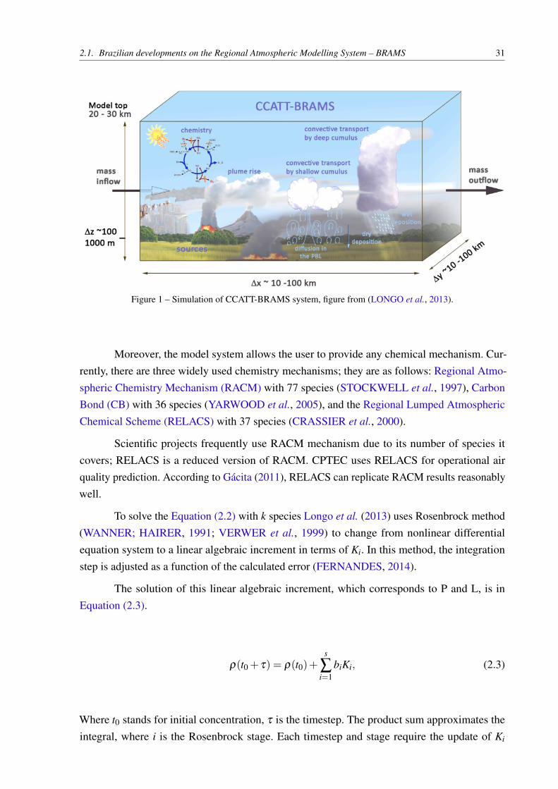
Unlike the GPU, where there are multiple cache levels, in FPGA local memory requiresM20K blocks spread over the board (INTEL, 2016a). In Figure 9, we show a local memory witha single bank and three M20K blocks.
Regarding private memory, Intel uses FPGA register to implement them. That is thefastest memory in the hierarchy, and there is a generous number of them in the FPGA. Thedevice can access these register in parallel, which allows a much higher bandwidth than any other
2.5. Intel FPGA SDK for OpenCL 43
Figure 9 – Implementation of local memory with three M20K blocks, figure from (INTEL, 2016a).
memory in OpenCL. According to our experiments, Intel infers registers for single variables orsmall arrays; a relative big array requires a local memory.
Intel performs several optimizations before generating the hardware, and Figure 10 showsthe flow of the compilation of OpenCL based on LLVM compiler infrastructure. The input is anOpenCL application (.cl) that contains a set of kernels and a host program (.c) (CZAJKOWSKIet al., 2012b).
Compilation of the host source code uses a standard C compiler. The compiled file linkswith Altera OpenCL (AOCL) Host Library. Regarding the kernel source code, it uses an offlinekernel compiler (JANIK; TANG; KHALID, 2015), i.e. the programmer must compile the kernelseparate from the host; this process may take hours to compile.
Compilation of the hardware is not as simple as it seems. A C-language parser outputsan LLVM Intermediate Representation (IR) for each kernel (in essence, kernel is a C code); thisintermediate representation is in the form of instructions and dependencies between them.
From this IR, the compiler optimizes it (live-value analysis) for an FPGA target. Afteroptimizing, a Control-Data Flow Graph (CDFG) conversion takes place. The conversion isnecessary to improve performance, reduce area and energy consumption before RTL generation(RTL generator) in Verilog for a kernel.
A system with interfaces to host and off-chip memory instantiates the compiled kernels.The host interface allows the host to access each kernel and specify workspace parameters andkernel arguments. Off-chip memory represents the global memory for a kernel in OpenCL, inour case, it is a DDR3 memory. Finally, we can synthesize the complete system in Figure 7 onan FPGA.
At last, the compiled host program has two elements. The first is the ACL Host Library;

44 Chapter 2. Fundamental Concepts
it calls the functions that allow the host application to exchange information with the FPGAkernels. The second is the auto-discovery that allows the host program to detect the kernels typeson an FPGA.
kernel.cl host.c
ACLC-Language
front end
AutoDiscovery C compiler
ACLHost
Library
program.exe
CDFG
Live-Value Analysis
Com
pile
r
CDFGGeneration
Scheduling
Ker
nel
RTL generatorVerilog
HDL
System Integration (Quartus II)
Figure 10 – Design flow with OpenCL, figure from (CZAJKOWSKI et al., 2012b).
The main advantage of OpenCL over the traditional Hardware Description Language(HDL) is to produce designs with proper functionality without the FPGA design effort (consider-ing the kernel is working correctly). Once the user has created a functional model, the focus ison the optimization. It is different from the HDL designs, where only in the design process wecan assure the correct functionality (JANIK; TANG; KHALID, 2015).
We present further implementation details in Chapter 3; we explain the pipelines of ourarchitectures, memory hierarchy, interoperability between the host and the device.
2.6 FPGA
In 1985, Xilinx introduced the FPGA (BOBDA, 2007). An FPGA is a semiconductordevice, which contains a two-dimension array of generic logic cells and programmable switches(CHU, 2011; MOORE ANDREW; WILSON, 2017). Over the years, the FPGAs has shown thatcapacity (number of gates) and speed are inversely proportional to price and power consumption,see Figure 11.
2.7. Development Environment for OpenCL 45
10,000x more logic–Plus embedded IP
• Memory• Microprocessor• DSP• Gigabit serial I/O
100x faster5,000x lower power 10,000x lower cost
10,000
1,000
100
10
1985 1990 1995 2000 2005 2010 2015
CapacitySpeedPricePower
1
Figure 11 – Xilinx field-programmable gate array (FPGA) progression. (Price and power are per logic cell.), figurefrom (AHMAD et al., 2016).
With an FPGA the programmer can define the behavior of the hardware after the manu-facturing, that is why the name field programmable. That is possible due to the logic cells thatcan perform the behavior of different functions; once defined the logic and synthesized, theprogrammer can download the design through a bus to the FPGA; this bus can be a simple USBcable (BOUT, 2011).
Modern FPGAs contain a set of configurable Static Random Access Memory (SRAM),high-speed input/output pins (I/Os), logic blocks, and routing. They also have many LogicElements (LE), which are the smallest unit of logic; usually, they are a Look-Up Table (LUT).Each LE can perform complex functions or simple basic logic as AND/OR. FPGAs also haveconfigurable memory blocks; these memory blocks allows the programmer to provide a higherthroughput since they are over the board.
Although FPGAs are reconfigurable, they also provide hard logic or hard IntellectualProperty (IP), i.e. that does not change. Those circuits implement specific logic consideredcommodity, which allows the programmer to reduce cost and power of the design. These featuresallowed the programmers to build complex systems called System-On-a-Programmable-Chip(SOPC).
In general, SOPC or System-On-Chip (SOC) focus on lower-power electronics or high-performance applications. According to Silva (2014), SOPC is a suitable option for high-performance computing.
2.7 Development Environment for OpenCLWe used Bittware S5PH-Q-A7 board available at the Reconfigurable Computing Lab-
oratory (LCR) at USP. In the next subsection, we further detail the main resources in this
46 Chapter 2. Fundamental Concepts
device.
2.7.1 BittWare Board S5PH-Q
S5PH-Q is a half-length x8 card based on the high-bandwidth and the power-efficientAltera Stratix V GX A7. Stratix V FPGA is suitable for high-end applications; according to(DINIGROUP, 2017), this board guarantees 5,410 millions of gates for use.
The S5PH-Q is a versatile and efficient solution for high-performance network processing,signal processing, and data acquisition (BITTWARE, 2015). LCR purchased this board for theprojects involving BRAMS and heterogeneous computing. Figure 12 shows the block diagramfor this device, in Table 2 we detail the features.
Figure 12 – Top-Level Component Implementation Block Diagram, figure from (BITTWARE, 2015).
2.8 Hardware/Software CodesignHardware/software codesign emerged in the 90’s as a discipline, however this task was al-
ready common among the microprocessor companies. At the time, they were not conscious of theterm codesign. Currently, a successful electronic system design requires the of hardware/softwarecodesign techniques (TEICH, 2012).
The current technology allows the programmers to deal with multiple processor cores,memory arrays, application specific hardware on a single chip (GALLERY, 2015). A more recentapproach is from Intel on the HARP (Heterogeneous Architecture Research Platform) program,which included a Intel microprocessor and a Stratix V FPGA (GUPTA, 2015).
Such evolution in the technology requires the programmers to have knowledge in hard-ware and software, thus they can define the design trade-offs. In this manner, hardware/softwarecodesign is becoming and ordinary task. In the literature we have some definition for hardware/-software codesign.
2.8. Hardware/Software Codesign 47
Table 2 – S5PH-Q Features
Device FeaturesAltera R○ Stratix R○ V GXFPGA
∙ 20 full-duplex, high-performance, multi-gigabit SerDestransceivers @ up to 14.1GHz
∙ 952,000 logic elements (LEs) available
∙ Up to 52 Mb of embedded memory
∙ 1.4 Gbps LVDS performance
∙ Up to 1,963 variable-precision DSP blocks
∙ Embedded HardCopy Blocks
Memory
∙ Two banks of 4 GBytes DDR3 SDRAM (1Gx64)
∙ Four banks of up to 18 MBytes QDRII/QDRII+(8M x 18)
∙ 128 MBytes of Flash memory for booting FPGA
PCIe Interface x8 Gen1, Gen2, Gen3 direct to FPGAUSB USB 2.0 interface for debug and programmingDebug Utility Header
∙ RS-232 port to Stratix V
∙ JTAG debug interface to Stratix V
QSFP+ Cages (optional) 2 QSFP+ cages on front panel connected to FPGA via 8 SerDesSize Half-length, standard-height PCIe slot card
According to Schaumont (2012), “Hardware/Software codesign is the design of cooperat-ing hardware components and software components in a single design effort.". Another definitionin the book is: “the activity of partitioning, where one partition holds the flexible part (software),and the other the fixed part (hardware)".
Gallery (2015) defines as a “concurrent design of both hardware and software of thesystem by taking into consideration the cost, energy, performance, speed and other parameters ofthe system".
Figure 13 shows the pros and cons of Hardware and Software. In Hardware, it is possibleto have a better performance, less energy consumption (more work done per unit of energy),power density (processors can no longer increase clock). In Software, design complexity is muchharder in hardware, design cost, shrinking design schedules (time-to-market is reducing over theyears, but software development can start even without a hardware platform).
48 Chapter 2. Fundamental Concepts
Figure 13 – Driving factors in hardware/software codesign, figure from (SCHAUMONT, 2012).
Partitioning or balancing is a hard task, and there is no magical solution. This workrequires experience; another important factor is the cost, many times it is better a cheaper productthan a fast product. Blickle, Teich and Thiele (1998) shows a theorem proving that determining afeasible allocation is a NP-Complete problem. In this work they consider the problem of mappinga set of tasks to resources.
There are some developed works on the literature that consider the hardware/softwarepartitioning. Gupta and Micheli (1993) automates the design space exploration; initially, thealgorithm of this work considers that all functionalities are in hardware and gradually moves tosome of them to software based on the communication overhead. The problem is that much ofthe initial problem requires many resources from the hardware, because the initial guess startsfrom the problem entirely in hardware.
Ernst, Henkel and Benner (1993) follows an opposite approach, they start with aninitial partition in software and gradually moves the software part into hardware. They used apartitioning heuristic, where the algorithm minimizes the amount of hardware resources. Theyshow good results for the partitioning of the digital control of a turbocharged diesel engine and afilter algorithm for a digital image compared to software.
2.9 Related WorkSparse matrices are necessary for several scientific and engineering applications. For ex-
ample, least squares problems, eigenvalue problems, and image reconstruction. When comparedto dense matrices, sparse matrices tend do be slower. The irregularity of memory access causesmany cache misses, and there is the fact that memories are still much slower than processors.Another source for this slowness, is the high ratio of load and store operations, stressing theload/store units (ZHUO; PRASANNA, 2005).
FPGAs can effectively compute sparse matrix. The modern FPGAs provide multiplespatial floating-point operators, a significant of high-bandwidth on-chip memory, and abundantI/O pins (KAPRE; DEHON, 2009).
Kapre and DeHon (2009) parallelizes a Sparse Matrix Solver for SPICE (SimulationProgram with Integrated Circuit Emphasis); the results range from 300 to 1300 MFlop/s on aXilinx Virtex-5, while the processor (Intel Core i7 965) achieved 6 to 500 MFlops/s. According

2.9. Related Work 49
to the authors, the former library (Sparse 1.3a) was not suitable for parallelization on FPGAsdue to the frequent change of the non-zero pattern of the matrix.
They used the KLU solver. Circuit simulations are suitable problems for this solver.According to Eller, Singh and Sandu (2010), LU decomposition is not easily parallelizable. Later,they integrated the solver to SPICE (KAPRE; DEHON, 2012). In this new version, they alsostudied the energy savings of their work, which ranges from 8.9× up to 40.9× compared toCPU. They provide a codesign between the MicroBlaze and their hardware; MicroBlaze haspoor support for double precision.
LU direct method emerged at the beginning of 2000 with Daga et al. (2004), Zhuo andPrasanna (2006). However, none of the works consider sparse matrices; which is the problemof BRAMS. In Wu et al. (2011), they compute the preprocessing in CPU and the numericfactorization in FPGA of the LU algorithm; they use sparse representation.
In Foertsch, Johnson and Nagvajara (2005), they consider the problem of Full-AC loadflow, an important task in power system analysis. In their work, they compare Jacobi methodto Newton-Raphson methods and conclude that Jacobi could outperform Newton method byexploring pipeline parallelism in FPGA. They do not consider any coupling to the load flowproblem, i.e. there is not codesign.
Morris and Prasanna (2005), Prasanna and Morris (2007) study a related problem toBRAMS, they solve Partial Differential Equations (PDE) discretized in a linear system (sparseand dense) in FPGA. They also consider a highly pipelined Jacobi; the algorithm represented infloating point with 64 bits. However, they fail to consider a better approach to fit bigger matrices,each column of the row requires a multiplier. In this manner, hardware resources are proportionalto matrix size.
When they need bigger matrices, they multiplex the entries to the underlying hardware.They also have problems with reduction, which required the implementation of an efficient one.The authors do not provide any circuit to test the convergence of the algorithm; they test theirhardware with a predefined number of iterations.
Kasbah and Damaj (2007) implements Jacobi method in Handel-C. According to them,the hardware of the method can outperform the same algorithm in Software. They validate theirtests by using the Handel-C simulator, i.e. they do not perform any test on the hardware. Theauthors also had to consider the algorithm in integer representation since Handel-C does notsupport floating point, and the library from Celoxica had some bugs to handle more than fourfloating point operations. In this dissertation, we do not simulate the results; all the computationsare in FPGA, which provides much more accurate results.
Bravo et al. (2006) proposes the use of Jacobi method to solve the Eigenvalue andEigenvector problems; a similar work is in Wang and Wei (2010). In the proposed architecture,they improve FPGA area by implementing the whole system in VHDL. They compare their

50 Chapter 2. Fundamental Concepts
results, represented in floating point with 18 bits, with the results of the CPU, represented infloating point with 64 bits, and conclude that their design is faster and provides accurate results.In this work there is no codesign, the entire execution is in hardware with pre-fixed values storedin ROM memory.
Ruan et al. (2013) presents a similar approach that we used in BRAMS; they use a high-level synthesis from Maxeller, where the programmer defines the kernel in Java and MaxCompileris responsible for creating a bitstream file. They also provide a codesign between CPU andFPGA; in their project, they provide a modification for Jacobi method called pipeline-friendlyJacobi.
According to their results, MaxCompiler generated a hardware that is capable of runningat 175Mhz on Virtex-6. They compared their results with three different configurations: FPGAv.s single-thread CPU, FPGA v.s multi-thread CPU, and FPGA v.s MPI CPU. We show theirspeedup results in Figure 14, as we can see FPGA is superior even with MPI parallelism. Matrixsize is a problem in their design, they cannot fit matrices bigger than 200×200 in the memory.
0
50
100
150
200
250
300
350
2 4 8 16 32 64 128 200
FPGA v.s single-thread CPU versionFPGA v.s multi-thread CPU versionFPGA v.s MPI CPU version
Figure 14 – Speedup compared to CPU versions. The x dimension stands for matrix size, and y dimension speedupin FPGA.
Schmid et al. (2014) proposes the use of the Heterogeneous Image Processing Acceler-ation Framework (HIPAcc) for Multiresolution Analysis (MRA). They use this framework togenerate code for the FPGA target; one of the case studies proposes Jacobi method as a smootherfor PDE. They achieved 154Mhz on a mid-range FPGA (Xilinx Zynq 7045).
Although the success regarding the results, their design suffers from the number of block

2.9. Related Work 51
RAMS. They cannot control the underlying hardware to reuse block RAM more efficiently. Thepragmas in the framework have a severe impact over the Initiation Interval (II) (SCHMID et al.,2014); however the framework does not offer any tool to help the programmer improve II.
An and Wang (2016) uses OpenCL for programming Singular Value Decomposition(SVD) in the AMD GPU. For computing SVD they used an adapted version of Jacobi methodcalled one-sided Jacobi method. According to Lambers (2010), one-sided Jacobi implicitlyapplies the Jacobi method for the symmetric eigenvalue problem.
In their work, they used a W9100 graphics card from AMD, and according to the authors,it was the best and fastest graphics card. They performed the same tests we did, i.e. they usesingle and multi-thread to program the kernel. For small matrices, they had a better executiontime single thread, for matrices with the order of 16 they had an improvement by using multiplethreads. In this work, they do not perform any study related to power consumption, according toAMD vendor, this board can consume up to 275W.
In Gomes (2009), they use Jacobi for fluid simulation by implementing the algorithmin CUDA. According to them, the algorithm suffers from global memory latency. In FPGA wecould improve this problem by using more local memory during computation since we can defineour local memory size (as long as it does not exceed the hardware capacity). We avoided suchproblem due to the small memory footprint of our problem.
Fernandes (2014) decided to solve the linear systems from chemical reactivity of BRAMSby using optimum linear estimation. The author implemented the algorithm in OpenMP andOpenACC, although they achieve good results in time execution and precision, they do notcouple their algorithm to BRAMS. According to Fazenda et al. (2006), coupling the chemicalreactivity to CCATT-BRAMS is a complex task.
Michalakes and Vachhrajani (2008) developed Kinetic PreProcessor (KPP) Rosenbrockchemical integrator for GPUs in CUDA. They converted WRF Single Moment 5-tracer (WSM5)to CUDA, a model that represent the microphysics of clouds and precipitation. Their GPU didnot provide double precision, so they needed to use single precision. Their implementation alsorequires a CPU per GPU. Their results show a speed-up of 1.23×, but they do not mention ifthis is due to the lower precision of the results.
Linford and Sandu (2009) used a Cell Broadband Engine Architecture (CBEA) to solvemass balance equations of Chemical transport model. They implemented a 3D chemical transportmodule for FIXED-GRID, this model also uses Rosenbrock method. Their work presents asuperlinear speed-up. However, their vector stream processing requires the kernel to process thedouble of computing that it needs.
According to the authors these useless arithmetic operations is crucial to sustaining ahigher throughput; otherwise branching conditions would be prohibitively expensive. Branchingis not a problem on FPGA since all code-paths are established in hardware (ACCELEWARE,
52 Chapter 2. Fundamental Concepts
2014).
Eller, Singh and Sandu (2010) also use Rosenbrock method to solve the chemical system.In their experiments, they use Rodas-3 and Rodas-4 methods. Although the names suggest thenumber of stages, Rodas-3 uses four stages and three function calls. Rodas-4 has six stages andfive function calls. They had to make significant changes in Rosenbrock data structure to fit thedata in a 16KB of local memory. Memory transfer is responsible for one-third of the overallrunning time.
According to the authors, Rosenbrock does not provide any speed-up for each iteration;in some cases, the results in GPU was slower. Their results point to the fact that local memory isthe main problem.
In Fu et al. (2017), they implement Shallow Water Equations solver in three differentarchitectures. One of them is CPU-FPGA, they had to decompose the solver in three FPGAs tofit the double precision version; this solution resulted in a low bandwidth among the FPGAs. Asecond approach involved the use of mixed precision, which resulted in a relative error of lessthan 2% and 80% of the resources of a single FPGA; they implemented their design by usingJava from MaxCompiler. This version had a speedup of 75× compared to CPU.
In Yang et al. (2016), they present an ultra scalable solution — in the order of 10M-core — for Fully-Implicit Solver for Nonhydrostatic Atmospheric Dynamics. They implement ahighly parallel incomplete LU method that does not sacrifice convergence rate in their SW26010processor.
In Table 4, we provide the main features of each work compared to our third architectureArch 3.
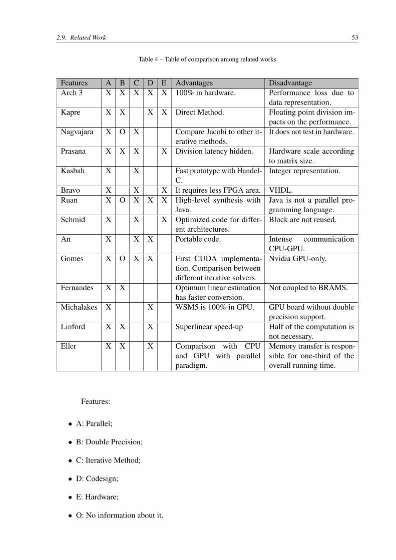
2.9. Related Work 53
Table 4 – Table of comparison among related works
Features A B C D E Advantages DisadvantageArch 3 X X X X X 100% in hardware. Performance loss due to
data representation.Kapre X X X X Direct Method. Floating point division im-
pacts on the performance.Nagvajara X O X Compare Jacobi to other it-
erative methods.It does not test in hardware.
Prasana X X X X Division latency hidden. Hardware scale accordingto matrix size.
Kasbah X X Fast prototype with Handel-C.
Integer representation.
Bravo X X X It requires less FPGA area. VHDL.Ruan X O X X X High-level synthesis with
Java.Java is not a parallel pro-gramming language.
Schmid X X X Optimized code for differ-ent architectures.
Block are not reused.
An X X X Portable code. Intense communicationCPU-GPU.
Gomes X O X X First CUDA implementa-tion. Comparison betweendifferent iterative solvers.
Nvidia GPU-only.
Fernandes X X Optimum linear estimationhas faster conversion.
Not coupled to BRAMS.
Michalakes X X WSM5 is 100% in GPU. GPU board without doubleprecision support.
Linford X X X Superlinear speed-up Half of the computation isnot necessary.
Eller X X X Comparison with CPUand GPU with parallelparadigm.
Memory transfer is respon-sible for one-third of theoverall running time.
Features:
∙ A: Parallel;
∙ B: Double Precision;
∙ C: Iterative Method;
∙ D: Codesign;
∙ E: Hardware;
∙ O: No information about it.

55
CHAPTER
3DEVELOPMENT OF THE CODESIGN FORTHE CHEMICAL REACTIVITY OF BRAMS
Currently, BRAMS bases on software and MPI parallelism. This project focus on thechemical reactivity term included in BRAMS (CCATT). According to Zhang et al. (2011) andLinford et al. (2009), chemical reactivity can represent 90% of the computational time. On Tupã(Cray XE6) CPTEC/INPE this term is responsible for 80% of computational time (FERNANDES,2014). In this chapter, we compare our approach with the implementation of BRAMS for solvingthe linear systems from the chemical reactivity.
3.1 CCATT–BRAMS softwareBRAMS solves the mass equation of the chemical reactivity term using Sparse1.3a.
This library in C decomposes Equation (2.5) into LU form. Figure 15 represents BRAMS (graysquare) and Sparse1.3a (yellow square); it is important to point out that we used BRAMS with asingle grid.
We divided Figure 15 into three regions for a better explanation of how chemical BRAMScouples with the reactivity. The blue outermost region represents the South America, accordingto Alisson (2016) the Brazilian model can apply the chemical reactivity to the South Americawith a 20km resolution and 3.5 days of anticipation. The grayish middlemost region exemplifiesBRAMS over the South America with only a single process, i.e. one process is responsible forcomputing the entire grid. The following yellowish inner region represents Sparse1.3a libraryinside the process. In Figure 16, we represent BRAMS with multiple processes, note that we stillhave a single grid.
Each MPI process computes its slice of the domain decomposition. The shaded areasare the ghost zones; these regions are necessary for solving the fluid dynamical equations, asa consequence, the nearest neighbors generate communications among them. The strongest

56 Chapter 3. Development of the Codesign for the Chemical Reactivity of BRAMS
South AmericaSingle Grid
Software
Figure 15 – Generic representation of BRAMS system with a single process. In this figure, we present BRAMSover the South America with a single grid, yellow square represents Sparse1.3 running for all the pointsover the grid.
South America
... Pn
P4P1 P2 P3
P8P5 P6 P7
P12P9 P10 P11
P9 P10
Figure 16 – Generic representation of BRAMS system with MPI processes. In this figure, we present BRAMS overthe South America with a single grid distributed over N processes, each process executes Sparse 1.3 forits set of points of the grid. The shaded areas are the ghost zones, i.e. the shared data area.

3.2. CCATT–BRAMS Codesign 57
communications happen between horizontal and vertical neighbors; diagonal neighbors haveless intensive communication (RODRIGUES et al., 2009).
MPI assigns each domain to only one process, the only shared areas are the ghostzones.The less shared area, the less the external communication among MPI processes. The setof processes is distributed over the processors of the nodes, on our environment set we have asingle node with four core processors.
Although BRAMS is in Fortran 90, it is possible to call C functions. However, theprogrammer must take some extra care with interoperability of both languages, in the nextsection we describe the main problems raised from this coupling.
3.1.1 Interoperability with Sparse1.3a
Sometimes it is necessary to mix different languages for a single executable; this usuallyhappens when the programmer couples a library to its program. BRAMS coupled sparse1.3a, aC library with Fortran-ready interface. So no extra effort was necessary to adapt the C library.
To use this library with BRAMS, the programmer must enable Fortran interface. Byenabling this option, Fortran programmers do not have to worry about interoperability problems,such as data type representation, arguments type (passed by reference or by value), and arrayrepresentation (Row- or column-major order).
3.2 CCATT–BRAMS CodesignJacobi iterative solver has a parallel nature, which makes it suitable for FPGA paral-
lelization (MORRIS; PRASANNA, 2005). The chemical kinetic process has diagonal matrices(ZHANG et al., 2011), for our set of tests we guarantee they are strict diagonally dominant,this is necessary for Jacobi method convergence. Figure 17 shows a generic representation ofBRAMS coupled to the hardware designed in OpenCL.
We implemented three versions of Jacobi method: Multi-threaded dense, Multi-threadedsparse, and single thread sparse. We describe them over the next subsections.
3.2.1 Jacobi Multi-threaded Dense
In our first attempt with Intel FPGA SDK, we programmed the FPGA using similarapproaches used for GPU OpenCL. In other words, we used the concept of several computingunits working in parallel to solve a problem in an SIMD mode. Although the source code isportable, performance is not, with this approach we support this affirmation.
We followed some of Intel best practices (INTEL, 2016a) for our first version, we avoidedthe divide operation for floating-point and used aligned memory in 64 bytes. This implementation

58 Chapter 3. Development of the Codesign for the Chemical Reactivity of BRAMS
South AmericaSingle Grid
Hardware
Figure 17 – Generic representation of BRAMS coupled to the Jacobi method in Hardware. In this figure, we presentBRAMS over the South America with a single grid, red square represents Jacobi hardware circuit. Suchcircuit computes all the points over the grid.
uses a dense representation of matrix A. Figure 18 shows the schematic of the first version ofJacobi Method.
Here we present m pipelines. Each pipeline can process different work-items fromvarious work-groups. During kernel compilation, we can choose two options for work group size:max_work_group_size and reqd_work_group_size. The first option is a hint of the maximumnumber of work items; the compiler must not exceed this number.
The second option is much more strict, and it does not let the compiler optimize thework-group size for the problem. Work-group size is the number of work items for each work-group. We tested both options, and the first generated the best hardware. Figure 19 depicts howwork-groups and work-items map to our linear system.
According to the Verilog generated by Altera compiler, the compiler issues two workgroups in hardware for a single compute unit, and all the remaining work groups are scheduled,i.e. two work-groups are executing at the same time. The option num_compute_units allows usto increase the number of hardware available, although Intel does not recommend to do so due tothe concurrent access to global memory. Each hardware group has three stats:
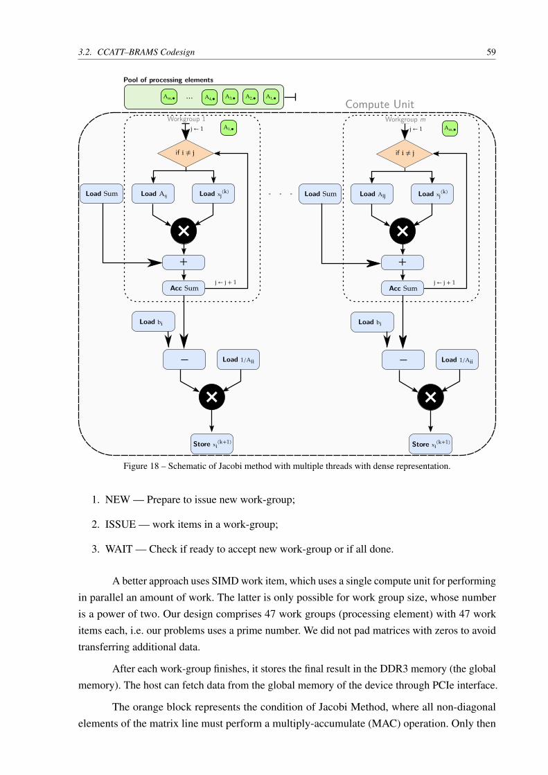
3.2. CCATT–BRAMS Codesign 59
Load xj(k)Load Sum
Am,⏺
Workgroup m
×
Load Aij Load xj(k)Load Sum
+
Acc Sum
j ← 1
j ← j + 1
Load bi
− Load 1/Aii
×
Store xi(k+1)
A1,⏺
Pool of processing elements
A2,⏺A3,⏺⋯ A4,⏺Am,⏺
A1,⏺
Workgroup 1
. . .
×
Load Aij
+
Acc Sum
j ← 1
j ← j + 1
Load bi
− Load 1/Aii
×
Store xi(k+1)
Compute Unit
if i ≠ j if i ≠ j
Figure 18 – Schematic of Jacobi method with multiple threads with dense representation.
1. NEW — Prepare to issue new work-group;
2. ISSUE — work items in a work-group;
3. WAIT — Check if ready to accept new work-group or if all done.
A better approach uses SIMD work item, which uses a single compute unit for performingin parallel an amount of work. The latter is only possible for work group size, whose numberis a power of two. Our design comprises 47 work groups (processing element) with 47 workitems each, i.e. our problems uses a prime number. We did not pad matrices with zeros to avoidtransferring additional data.
After each work-group finishes, it stores the final result in the DDR3 memory (the globalmemory). The host can fetch data from the global memory of the device through PCIe interface.
The orange block represents the condition of Jacobi Method, where all non-diagonalelements of the matrix line must perform a multiply-accumulate (MAC) operation. Only then
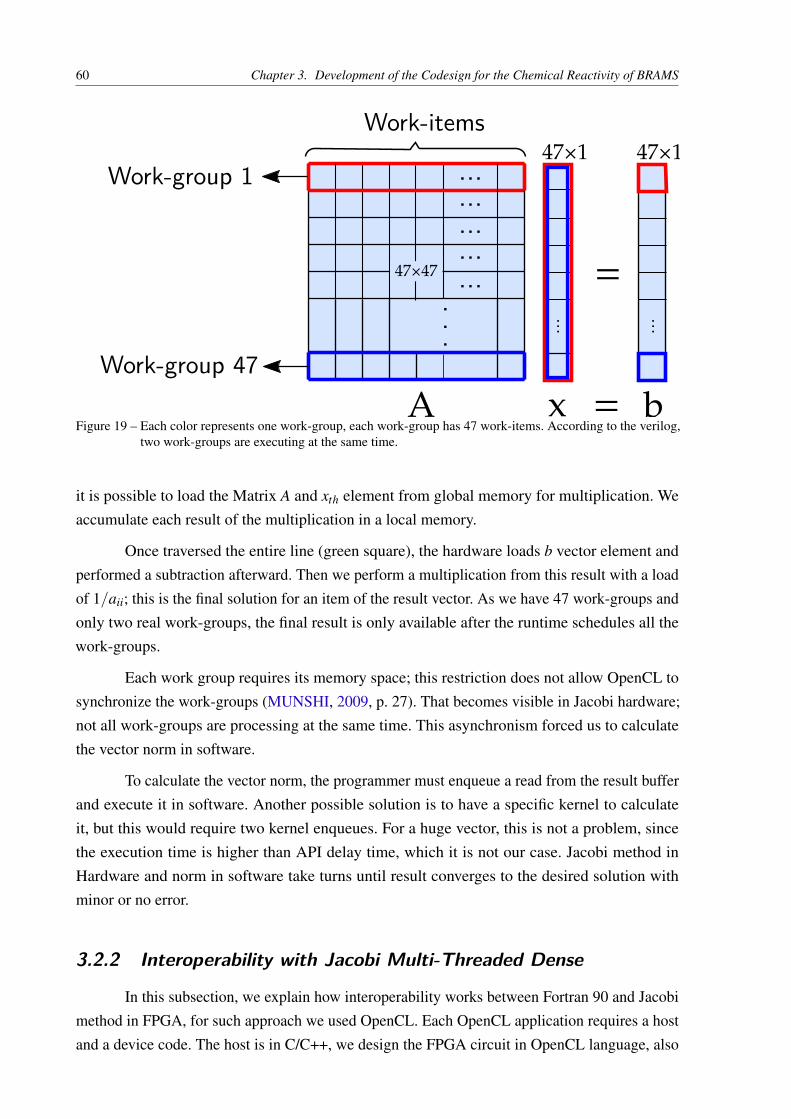
60 Chapter 3. Development of the Codesign for the Chemical Reactivity of BRAMS
47×47
. . .
Work-group 1
Work-group 47
...
...
...
...
...
Work-items47×1 47×1
A x = b
=
... ...
Figure 19 – Each color represents one work-group, each work-group has 47 work-items. According to the verilog,two work-groups are executing at the same time.
it is possible to load the Matrix A and xth element from global memory for multiplication. Weaccumulate each result of the multiplication in a local memory.
Once traversed the entire line (green square), the hardware loads b vector element andperformed a subtraction afterward. Then we perform a multiplication from this result with a loadof 1/aii; this is the final solution for an item of the result vector. As we have 47 work-groups andonly two real work-groups, the final result is only available after the runtime schedules all thework-groups.
Each work group requires its memory space; this restriction does not allow OpenCL tosynchronize the work-groups (MUNSHI, 2009, p. 27). That becomes visible in Jacobi hardware;not all work-groups are processing at the same time. This asynchronism forced us to calculatethe vector norm in software.
To calculate the vector norm, the programmer must enqueue a read from the result bufferand execute it in software. Another possible solution is to have a specific kernel to calculateit, but this would require two kernel enqueues. For a huge vector, this is not a problem, sincethe execution time is higher than API delay time, which it is not our case. Jacobi method inHardware and norm in software take turns until result converges to the desired solution withminor or no error.
3.2.2 Interoperability with Jacobi Multi-Threaded Dense
In this subsection, we explain how interoperability works between Fortran 90 and Jacobimethod in FPGA, for such approach we used OpenCL. Each OpenCL application requires a hostand a device code. The host is in C/C++, we design the FPGA circuit in OpenCL language, also

3.2. CCATT–BRAMS Codesign 61
called OpenCL C programming language (MUNSHI et al., 2011).
As we saw in Subsection 3.1.1, it is possible to call a C function from Fortran. However,now we had to take care with data type representation (double or Real*8); arguments fromFortran are passed by reference, in C they are passed by value; array representation in Fortran iscolumn-major, in C they are row-major. Indices in Fortran start from 1, not 0.
In this version, we solved one linear system at a time. That is the same approach used bySparse1.3a. In fact, we replaced the previous sparse function to ours.
For using our solver, we first needed to reprogram the FPGA on the system. We guaranteethat with two similar approaches. The first requires the programmer to load the FPGA binary(AOCX) in advance through Intel SDK command, and set a variable:
1 $ a o c l program < dev ice > < f i l e > . aocx2 $ export CL_CONTEXT_COMPILER_MODE_ALTERA=3
The second reprograms the FPGA during runtime on the creation of program structure.It is user’s decision to choose what is the best approach. Usually, the delay of reprogramming isabout one or two seconds. Because of this overhead, we put all the kernel definitions in a singlecl file.
After reprogramming, BRAMS execution starts and when it gets to chemical reactivity itstarts solving the matrices through FPGA circuit designed in OpenCL. Apart from creating thenecessary OpenCL structures, we use C language as a bridge between Fortran and FPGA circuit.Figure 20 shows how BRAMS calls the circuit. Different from the GPU, our cl file represents aphysical circuit in FPGA not software.
Fortran 90 File C file
SUBROUTINE Solve_linear
CALL solver_jacobi_fpgaEnqueueNDRange(jacobi_method)
Load xj(k)Load Sum
Am,⏺
Workgroup m
×
Load Aij Load xj(k)Load Sum
+
Acc Sum
j ← 1
j ← j + 1
Load bi
− Load 1/Aii
×
Store xi(k+1)
A1,⏺
Pool of processing elements
A2,⏺A3,⏺⋯ A4,⏺Am,⏺
A1,⏺
Workgroup 1
. . .
×
Load Aij
+
Acc Sum
j ← 1
j ← j + 1
Load bi
− Load 1/Aii
×
Store xi(k+1)
Compute Unit
Skip if i = j Skip if i = j
Figure 20 – Interoperability of BRAMS and OpenCL. Fortran calls a function from the C host, which in turn isresponsible to manage the device.
As we can see, software and hardware have a strong communication. The C file is on thehost processor, and it is responsible for calculating the vector norm for each iteration of Jacobi.If the result did not converge, we send all the necessary data and NDRange. A host that usesNDRange bigger than 1 expects a circuit with data parallelism.
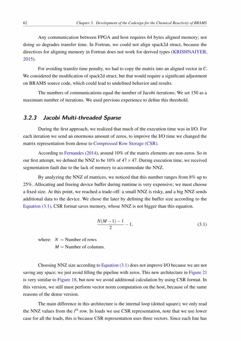
62 Chapter 3. Development of the Codesign for the Chemical Reactivity of BRAMS
Any communication between FPGA and host requires 64 bytes aligned memory; notdoing so degrades transfer time. In Fortran, we could not align spack2d struct, because thedirectives for aligning memory in Fortran does not work for derived types (KRISHNAIYER,2015).
For avoiding transfer time penalty, we had to copy the matrix into an aligned vector in C.We considered the modification of spack2d struct, but that would require a significant adjustmenton BRAMS source code, which could lead to undefined behavior and results.
The numbers of communications equal the number of Jacobi iterations; We set 150 as amaximum number of iterations. We used previous experience to define this threshold.
3.2.3 Jacobi Multi-threaded Sparse
During the first approach, we realized that much of the execution time was in I/O. Foreach iteration we send an enormous amount of zeros, to improve the I/O time we changed thematrix representation from dense to Compressed Row Storage (CSR).
According to Fernandes (2014), around 10% of the matrix elements are non-zeros. So inour first attempt, we defined the NNZ to be 10% of 47×47. During execution time, we receivedsegmentation fault due to the lack of memory to accommodate the NNZ.
By analyzing the NNZ of matrices, we noticed that this number ranges from 8% up to25%. Allocating and freeing device buffer during runtime is very expensive; we must choosea fixed size. At this point, we reached a trade-off: a small NNZ is risky, and a big NNZ sendsadditional data to the device. We chose the later by defining the buffer size according to theEquation (3.1), CSR format saves memory, whose NNZ is not bigger than this equation.
N(M−1)−12
−1, (3.1)
where: N = Number of rowsM = Number of columns.
Choosing NNZ size according to Equation (3.1) does not improve I/O because we are notsaving any space; we just avoid filling the pipeline with zeros. This new architecture in Figure 21is very similar to Figure 18, but now we avoid additional calculation by using CSR format. Inthis version, we still must perform vector norm computation on the host, because of the samereasons of the dense version.
The main difference in this architecture is the internal loop (dotted square); we only readthe NNZ values from the ith row. In loads we use CSR representation, note that we use lowercase for all the loads, this is because CSR representation uses three vectors. Since each line has

3.2. CCATT–BRAMS Codesign 63
Load xjaj
(k)Load Sum
Am,⏺
Workgroup m
×
Load aj Load xjaj
(k)Load Sum
+
Acc Sum
j ← start
j ← j + 1
Load bi
− Load 1/Aii
×
Store xi(k+1)
A1,⏺
Pool of processing elements
A2,⏺A3,⏺⋯ A4,⏺Am,⏺
A1,⏺
Workgroup 1
. . .
×
Load aj
+
Acc Sum
j ← start
j ← j + 1
Load bi
− Load 1/Aii
×
Store xi(k+1)
Compute Unit
if i ≠ j if i ≠ j
Figure 21 – Schematic of Jacobi method with multiple threads with sparse representation.
its NNZ size, we defined each group to have one work item to process each line; we show thisscheme in Figure 22.
3.2.4 Interoperability with Jacobi Multi-Threaded Sparse
Changing the matrix representation required few modifications on host code. We added aC algorithm for converting from dense representation to CSR; we called dnscsr_c,this functionrelies on the dnscsr algorithm from Sparsekit 1.
Sparsekit dnscsr function is in Fortran 90, using this library does not require any modi-fication to BRAMS source code. We decided to rewrite this function in C to avoid managingdifferent source codes.
Refactoring the algorithm added the burden of managing row- and column-major order
1 <https://people.sc.fsu.edu/~jburkardt/f_src/sparsekit/sparsekit.html>

64 Chapter 3. Development of the Codesign for the Chemical Reactivity of BRAMS
...
Work-group 0 Work-group 1 Work-group n
Work-item 0 Work-item 1 Work-item n
47×1 47×1
x = b
=... ...
1×NNZa
Figure 22 – Each color represents one work-group, each work-group has one work-item. In this manner, the numberof work-items is equal to the number of work-groups.
of matrix A. So in Fortran we passed the transposed matrix of A to dnscsr_c; we used transposefor simplicity of the algorithm in C, and avoid undefined behavior. This is not a problem, sincewe are not using dense representation.
As we told in Subsection 3.2.3, the NNZ varies from one matrix to another. So it isnot possible to determine a single size of the vectors Value and JA. Allocating and freeingmemory for each matrix is not a good option either, since this increases execution time. So, inour approach, we declare three vectors Value, IA, and JA, where Value and JA have fixed sizeaccording to Equation (3.1).
The host code of OpenCL uses these vectors that come from Fortran. Thus, we avoidcreating them for each matrix during execution. Fortran is also responsible for calling dnscsr_cbefore any call to Jacobi Multi-threaded Sparse solver.
3.2.5 Jacobi Single-threaded Sparse
According to Intel (2016a), sharing fine-grained data is not suitable for data parallelprogramming model. In these cases, using a single thread kernel can offer a higher throughput.
In the two previous architectures we could not compute vector norm, due to the restrictionof different memory space for each work group; and consequently, we are not able to sharememory.
In a single thread; we can compute vector norm because in this case, OpenCL workslike a C to Hardware. We can also avoid dispatching multiple times the same data from CPU to
3.2. CCATT–BRAMS Codesign 65
FPGA since we can define in our kernel to execute Jacobi until the matrix converges.
For using single thread kernel, we must set reqd_work_group_size (1,1,1) and not useget_global_id. When designing the hardware as a single thread, the programmer must declarethe variable in the deepest scope possible; otherwise, it will consume more hardware resourcethan it needs. AOCL (Altera OpenCL) generates a detailed report containing the depth of thevariables; we improved the depth of our variables through this report.
Regarding loop pipelining, single kernel executes multiple iterations in flight. Not allloops are capable of pipelining; the outermost loop (plain square), responsible for controllingthe iterations of the algorithm, is an example. The algorithm demands the loop to stop when itconvergences since each matrix have different stop criteria the compiler cannot infer any order.
CSR format adds a complex loop exit condition in the pipeline (dotted red square)since each row has different NNZ; Note the red border square, it means that it is necessarytwo loads. Another problem is the loop-carried dependency on the sum accumulator. Suchcondition, multiple loads, and loop-carried dependency degrade loop pipeline performancebecause subsequent iterations cannot launch until the previous one completes. So for Jacobisingle sparse, dot product is the bottleneck.
During vector norm calculation (innermost dotted black square) we also have a loop-carried dependency on the accumulator, but now there is a well-formed loop. That is, the loop isalways the same independent of iteration. Such loop allows us to remove it by inferring shiftregisters. So the vector norm calculation becomes parallel. In Figure 23, we show the pipelinesfor Jacobi.
Besides the different architecture, this kernel is 100% in hardware. So we do not avoidany expensive operation; we used built-in functions for power and square root calculation. Thisarchitecture represents the Jacobi method algorithm in hardware, totally independent from thehost processor.
Figure 23 shows a single compute unit. Although the compiler allows the programmer toinfer more compute units in a single kernel, the behavior does not make sense. Define more thanone compute unit for a single thread kernel means the same calculation over different circuits.Different from NDRange, the amount of work is not divisible.
Each matrix belongs to a single kernel; the programmer can increase throughput byreplicating the kernels manually and calling them with different queues and matrices on the host.As already stated in the previous architectures, the programmer must consider if this a goodapproach due to memory competition.

66 Chapter 3. Development of the Codesign for the Chemical Reactivity of BRAMS
Load xjaj
(k)Load Sum
Pool of processing elements
a2a3⋯ a4am
a1
×
Load aj
+
Acc Sumj ← j + 1
Load bi
− Load 1/Aii
×
Store xi(k+1)
if (i ≠ j) ∧ (j < size)
j ← start
Single Compute Unit
i ← i + 1
i ← 1
Load xi(k-1)
−
+
Acc Conv
Load xi(k)
Square
i ← i + 1
SqrtConv
if Conv < 1e-7
Converged
it ← 1
it ← it + 1
if it < maxIt
if i < size
i ← 1
if i < size
Figure 23 – Schematic of Sparse Jacobi method with single thread.
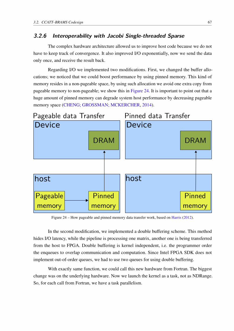
3.2. CCATT–BRAMS Codesign 67
3.2.6 Interoperability with Jacobi Single-threaded Sparse
The complex hardware architecture allowed us to improve host code because we do nothave to keep track of convergence. It also improved I/O exponentially, now we send the dataonly once, and receive the result back.
Regarding I/O we implemented two modifications. First, we changed the buffer allo-cations; we noticed that we could boost performance by using pinned memory. This kind ofmemory resides in a non-pageable space, by using such allocation we avoid one extra copy frompageable memory to non-pageable; we show this in Figure 24. It is important to point out that ahuge amount of pinned memory can degrade system host performance by decreasing pageablememory space (CHENG; GROSSMAN; MCKERCHER, 2014).
Pageable data Transfer Pinned data Transfer
Pageablememory
Pinnedmemory
DRAM DRAM
Pinnedmemory
host host
Device Device
Figure 24 – How pageable and pinned memory data transfer work, based on Harris (2012).
In the second modification, we implemented a double buffering scheme. This methodhides I/O latency, while the pipeline is processing one matrix, another one is being transferredfrom the host to FPGA. Double buffering is kernel independent, i.e. the programmer orderthe enqueues to overlap communication and computation. Since Intel FPGA SDK does notimplement out-of-order queues, we had to use two queues for using double buffering.
With exactly same function, we could call this new hardware from Fortran. The biggestchange was on the underlying hardware. Now we launch the kernel as a task, not as NDRange.So, for each call from Fortran, we have a task parallelism.


69
CHAPTER
4RESULTS
In this chapter, we present the profiling from BRAMS. In this profiling we confirm thatthe chem term is the most expensive equation in the mass continuity equation. Then we show theexperiments with the hardware in FPGA to solve the linear system from this equation.
We perform three experiments, one for each architecture of Jacobi method, we alsopresent the results from Sparse1.3a. We used the same heterogeneous machine we used forprofiling BRAMS. Regarding the analysis, we discuss precision, time execution, and energy.
4.1 Result analysis
We used Gprof to profile BRAMS under two configurations: with the chemical moduleenabled, and with the chemical module disabled. Such configuration is possible through theRAMSIN file, the input configuration file. We discuss the results below.
In the first configuration, we realized that the function radrrtm_ is responsible for 68%of the total time of computation. That is the only function that exceeds 3% of the total time.
On Figure 25 we can see the call graph, we generated this graphic representation withgprof2dot. It is important to point out that this call graph is not complete, we defined somethresholds to make the call graph fit the page. For this discussion, this call graph is enough.
When we enable the chemical module, we note that rodas-3 from Rosenbrock methodtakes about 41% of the total time. We represented the call graph on Figure 26; again this is apartial call graph.
The second heaviest function is spFactor; it is responsible for 17% of the total time. Thisfunction decomposes the matrix in LU format, as we mentioned earlier this decomposition isO(n3). By comparing the call graph in Figure 25 with Figure 26, we noted that solving linearsystems in rodas-3 are two times more expensive than computing radiation.

70 Chapter 4. Results
MAIN
__
97.6
8%
(0.0
0%
)1×
modonepro
c_m
p_onepro
c_
97.6
8%
(0.0
0%
)1× 97.6
8%
1×
modtim
este
p_m
p_tim
este
p_
97.5
0%
(0.0
0%
)288×
97.5
0%
288×
radia
tion_m
p_ra
dia
te_
76.0
8%
(0.0
0%
)288×
76.0
8%
288×
diffu
se_
8.4
7%
(0.1
5%
)288×
8.4
7%
288×
adve
ctc
_6.1
6%
(0.1
4%
)576×
6.1
6%
576×
mic
ro_
1.8
0%
(0.0
2%
)288×
1.8
0%
288×
modacoust_
mp_acoustic
_new_
1.7
6%
(0.0
0%
)288×
1.7
6%
288×
exevo
lve_
1.2
5%
(0.0
3%
)864×
1.2
5%
864×
main
97.6
8%
(0.0
0%
)
97.6
8%
1×
radrrtm
_76.0
3%
(67.8
4%
)18×
76.0
3%
18×
diffs
clr_
6.2
4%
(2.3
7%
)4320×
6.2
4%
4320×
diffve
l_1.0
7%
(0.4
9%
)288×
1.0
7%
288×
stra
in_
0.6
2%
(0.1
1%
)288×
0.6
2%
288×
fa_xc_
1.7
2%
(1.7
2%
)4608×
1.6
2%
4320×
fa_yc_
1.6
9%
(1.6
9%
)4608×
1.5
9%
4320×
fa_zc_
1.6
1%
(1.6
1%
)4608×
1.5
1%
4320×
vel_
adve
ctc
_0.7
8%
(0.7
8%
)288×
0.7
8%
288×
mcphys_
1.1
6%
(0.0
5%
)968832×
1.1
6%
968832×
range_check_
0.5
5%
(0.5
5%
)968832×
0.5
5%
968832×
modacoust_
mp_acoust_
new_
1.7
5%
(0.0
0%
)288×
1.7
5%
288×
adve
ct_
theta
_0.6
7%
(0.0
0%
)288× 0.6
7%
288×
rrtmg_sw_ra
d_m
p_rrtm
g_sw_
6.1
5%
(0.1
5%
)18× 6.1
5%
18×
rrtmg_lw
_ra
d_m
p_rrtm
g_lw
_1.9
9%
(0.1
0%
)18×
1.9
9%
18×
rrtmg_sw_spcvm
c_m
p_spcvm
c_sw_
5.4
2%
(1.9
0%
)60552×
5.4
2%
60552×
rrtmg_lw
_rtrn
mc_m
p_rtrn
mc_
0.8
3%
(0.8
3%
)60552×
0.8
3%
60552×
rrtmg_lw
_ta
um
ol_
mp_ta
um
ol_
0.7
6%
(0.0
0%
)60552×
0.7
6%
60552×
gra
d_
2.4
5%
(0.0
0%
)10944×
1.9
4%
8640×
divc
art_
2.3
2%
(0.0
0%
)10368×
1.9
4%
8640×
0.3
9%
1728×
0.5
2%
2304×
ram
s_gra
d_
4.7
8%
(0.0
0%
)21312×
2.4
5%
10944×
2.3
2%
10368×
rrtmg_sw_vrtq
dr_
mp_vrtq
dr_
sw_
1.9
1%
(1.9
1%
)13563648×
1.9
1%
13563648×
rrtmg_sw_re
ftra_m
p_re
ftra_sw_
1.2
2%
(1.2
2%
)13563648×
1.2
2%
13563648×
gra
dyv_
1.2
6%
(1.2
6%
)5184×
1.2
6%
5184×
gra
dxu_
1.2
4%
(1.2
4%
)5184×
1.2
4%
5184×
gra
dyt_
1.1
3%
(1.1
3%
)5184×
1.1
3%
5184×
gra
dxt_
1.1
1%
(1.1
1%
)5184×
1.1
1%
5184×
modacoust_
mp_prd
ctp
1_
0.6
7%
(0.6
7%
)864×
0.6
7%
864×
exth
vadv_
0.6
5%
(0.0
2%
)288×
0.6
5%
288×
0.1
1%
288×
0.1
1%
288×
0.1
0%
288×
Figure 25 – Call Graph for BRAMS with chemical module disabled.
4.2 Experiments
We performed the experiments on a heterogeneous machine. Currently, we have a singlenode for testing BRAMS execution with FPGA. In this single node, we must run BRAMS with a

4.2. Experiments 71
MAIN__81.45%(0.00%
)1×
modoneproc_mp_oneproc_81.45%(0.00%
)1× 81.45%
1×
modtimestep_mp_timestep_81.28%(0.00%
)1440× 81.28%
1440×
module_chemistry_driver_mp_chemistry_driver_42.38%(0.00%
)5760×
42.38%5760×
carma_driv_mp_carma_driver_16.25%(0.00%
)1440×
16.25%1440×
monotonic_adv_mp_advmnt_driver_11.74%(0.00%
)1440×
11.74%1440×
diffuse_3.44%(0.08%
)1440× 3.44%
1440×
micro_thompson_2.56%(0.00%
)1440×
2.56%1440×
chemdrydepdriver_mp_drydep_driver_2.10%(0.00%
)1440×
2.10%1440×
chemsourcesdriver_mp_sources_driver_1.03%(0.00%
)1440×
1.03%1440×
main81.45%(0.00%
)
81.45%1×
mod_chem_spack_rodas3_dyndt_mp_chem_rodas3_dyndt_41.05%(7.24%
)360×
41.05%360×
modtuvdriver_mp_tuvdriver_1.33%(0.52%
)72× 1.33%
72×
rad_carma_mp_radcomp_carma_16.24%(0.00%
)72×
16.24%72×
monotonic_adv_mp_advect_mnt_11.52%(0.28%
)79200×
11.52%79200×
diffsclr_3.00%(1.52%
)79200×
3.00%79200×
brams_to_mic_thompson_2.55%(0.32%
)4844160×
2.55%4844160×
module_dry_dep_mp_dry_dep_2.10%(0.03%
)1440×
2.10%1440×
chem_sources_mp_sources_0.74%(0.00%
)1440× 0.74%
1440×
solve_sparse_mp_fact_solve_matrix_21.22%(0.02%
)169416100×
21.22%169416100×
solve_sparse_mp_solve_linear_9.64%(0.02%
)169416100×
9.64%169416100×
mod_chem_spack_jacdchemdc_mp_jacdchemdc_1.84%(1.49%
)643047× 1.84%
643046×
mod_chem_spack_fexchem_mp_fexchem_0.94%(0.43%
)1966200×
0.94%1966200×
modtuv_mp_tuv_0.81%(0.17%
)132514× 0.81%
132514×
spFactor17.58%(17.58%
)169416100×
17.58%169416100×spSolve
3.62%(3.62%
)169416100×
3.62%169416100×
solve_sparse_mp_load_matrix_7.14%(3.40%
)169416100×
7.14%169416100×
spClear2.48%(2.48%
)169416101×
2.48%169416100×
mod_chem_spack_rates_mp_rates_0.51%(0.51%
)1966200× 0.51%
1966200×
rad_carma_mp_radcarma_16.24%(0.02%
)242208×
16.24%242208×
rad_carma_mp_radtran_14.40%(0.22%
)484416×
14.40%484416×
rad_carma_mp_initrad_1.30%(0.00%
)484416×
1.30%484416×
rad_carma_mp_oppr_8.54%(8.54%
)484416×
8.54%484416×
rad_carma_mp_add_2.31%(2.31%
)484416×
2.31%484416×
rad_carma_mp_newflux1_1.84%(1.84%
)484416× 1.84%
484416×
rad_carma_mp_twostr_1.34%(1.34%
)484416×
1.34%484416×
rad_carma_mp_setuprad_1.30%(1.30%
)484416×
1.30%484416×
monotonic_adv_mp_advec3d_z_4.26%(4.26%
)79200×
4.26%79200×
monotonic_adv_mp_advec3d_y_2.80%(2.80%
)79200×
2.80%79200×
monotonic_adv_mp_advec3d_x_2.61%(2.61%
)79200× 2.61%
79200×
monotonic_adv_mp_advec3d_z_sedim_1.56%(1.56%
)40320×
1.56%40320×
sfadd1real_3.74%(3.74%
)1469075172× 3.74%
1469075172×
grad_0.79%(0.00%
)169920× 0.74%
158400×
divcart_0.78%(0.00%
)167040×
0.74%158400×
rams_grad_1.57%(0.00%
)336960×
0.79%169920×
0.78%167040×
module_mp_thompson_mp_mp_gt_driver_1.98%(0.11%
)4844160×
1.98%4844160×
module_mp_thompson_mp_mp_thompson_1.87%(1.65%
)4844160× 1.87%
4844160×
module_dry_dep_mp_dry_dep_sedim_particles_1.75%(0.04%
)1440×
1.75%1440×
module_dry_dep_mp_sedim_particles_3d_1.58%(1.58%
)1440× 1.58%
1440×
Figure 26 – Call Graph for BRAMS with chemical module enabled.
single MPI process.
According to HRZ (2017), the fine-grained scheduling available in GPU is not presenton the FPGA circuit generated by Intel OpenCL SDK, i.e. two processes cannot share the FPGAcircuit. Even with this information, we decided to perform some tests to reinforce this affirmation.
In our first attempt, we replicated the kernel for each MPI process. That requires theknowledge of how many processes will access the device simultaneously. Figure 27 shows the

72 Chapter 4. Results
schematic for our explanation using two processes.
P1 P2
Load xjaj
(k)Load Sum
Pool of processing elements
a2a3⋯ a4am
a1
×
Load aj
+
Acc Sumj ← j + 1
Load bi
− Load 1/Aii
×
Store xi(k+1)
if (i ≠ j) ∧ (j < size)
j ← start
Single Compute Unit
i ← i + 1
i ← 1
Load xi(k-1)
−
+
Acc Conv
Load xi(k)
Square
i ← i + 1
SqrtConv
if Conv < 1e-7
Converged
it ← 1
it ← it + 1
if it < maxIt
if i < size
i ← 1
if i < size
FPGAFigure 27 – Each MPI process accesses a copy of the kernel (an FPGA circuit).
For using this scheme, FPGA reconfiguration must occur before BRAMS execution.Otherwise, both processes try to reconfigure the same FPGA and a deadlock occurs. Duringexecution, we realized that this approach is not feasible; the second MPI process is not able tocontinue execution because Intel FPGA SDK kills it.
We tried another method; we decided to share OpenCL structures by using inter-processshared memory in Linux1. Figure 28 shows that each process has a private Context and Queue,we share program, device, and memory. We can see the program as a set of FPGA circuits, whereeach circuit represents a kernel. The device represents the FPGA board; each process declares amemory region inside the FPGA (device), in the figure we represent them as two purple boxes.
The first problem arose from this approach was the execution order of the MPI processes.MPI does not impose any order in its pool of processes; we needed to execute the master processbefore any other process. The master process was responsible for creating the shared region.During our tests, with two processes, we could infer an order randomly.
Considering the cases where there was order among processes, we still reached the Intelruntime restriction. Regarding the out-of-order cases, a segmentation fault occurred becausethere was no program structure.
We tried to avoid this problem by using a mixed approach. We programmed the FPGAbefore BRAMS execution, as we tried in the first approach, and execute BRAMS with shared1 http://man7.org/linux/man-pages/man7/shm_overview.7.html

4.3. Results from Jacobi Multi-threaded Dense 73
OpenCL
Queue 1Program
Load xjaj
(k)Load Sum
Pool of processing elements
a2a3⋯ a4am
a1
×
Load aj
+
Acc Sumj ← j + 1
Load bi
− Load 1/Aii
×
Store xi(k+1)
if (i ≠ j) ∧ (j < size)
j ← start
Single Compute Unit
i ← i + 1
i ← 1
Load xi(k-1)
−
+
Acc Conv
Load xi(k)
Square
i ← i + 1
SqrtConv
if Conv < 1e-7
Converged
it ← 1
it ← it + 1
if it < maxIt
if i < size
i ← 1
if i < size
K1
Load xjaj
(k)Load Sum
Pool of processing elements
a2a3⋯ a4am
a1
×
Load aj
+
Acc Sumj ← j + 1
Load bi
− Load 1/Aii
×
Store xi(k+1)
if (i ≠ j) ∧ (j < size)
j ← start
Single Compute Unit
i ← i + 1
i ← 1
Load xi(k-1)
−
+
Acc Conv
Load xi(k)
Square
i ← i + 1
SqrtConv
if Conv < 1e-7
Converged
it ← 1
it ← it + 1
if it < maxIt
if i < size
i ← 1
if i < size
Program
K2
Load xjaj
(k)Load Sum
Pool of processing elements
a2a3⋯ a4am
a1
×
Load aj
+
Acc Sumj ← j + 1
Load bi
− Load 1/Aii
×
Store xi(k+1)
if (i ≠ j) ∧ (j < size)
j ← start
Single Compute Unit
i ← i + 1
i ← 1
Load xi(k-1)
−
+
Acc Conv
Load xi(k)
Square
i ← i + 1
SqrtConv
if Conv < 1e-7
Converged
it ← 1
it ← it + 1
if it < maxIt
if i < size
i ← 1
if i < size
Device - Bittware (FPGA)
Memory 1 Buffer 1
Buffer 2Buffer n
Queue 2
Context 2
Context 1 Shared Resource
Memory 2Buffer 1
Buffer 2Buffer n
Figure 28 – OpenCL data structures – Program, Device and Memory buffers are shared among MPI processes.
memory. This approach did not require to make any modification to BRAMS source code.Although we avoid the order problem, runtime still kills the second process. These tests couldconfirm that each device requires a single process access.
4.3 Results from Jacobi Multi-threaded Dense
In our first design, we programmed our FPGA as GPU, i.e. we used the concept of severalworking units working parallel. Despite the difficulty to understand, this programming model isvery common for parallel programming, and we found several tutorials teaching how to programsimple problems in OpenCL. Jacobi method is similar to matrix-vector multiplication, a generaloperation in OpenCL programming.
During this approach, we realized the host is as important as the kernel. In this attempt,we committed several errors that led to a severe degradation in performance. We will discuss thekernels problems, and then host problems.
The memory hierarchy is critical regarding kernel programming. We have three memorytypes: Global, Local and Private memory. We tried to use the general practice of avoidingmemory access to global memory by copying the contents to a local memory.
Our designs usually had a higher frequency when we avoided this practice, after some
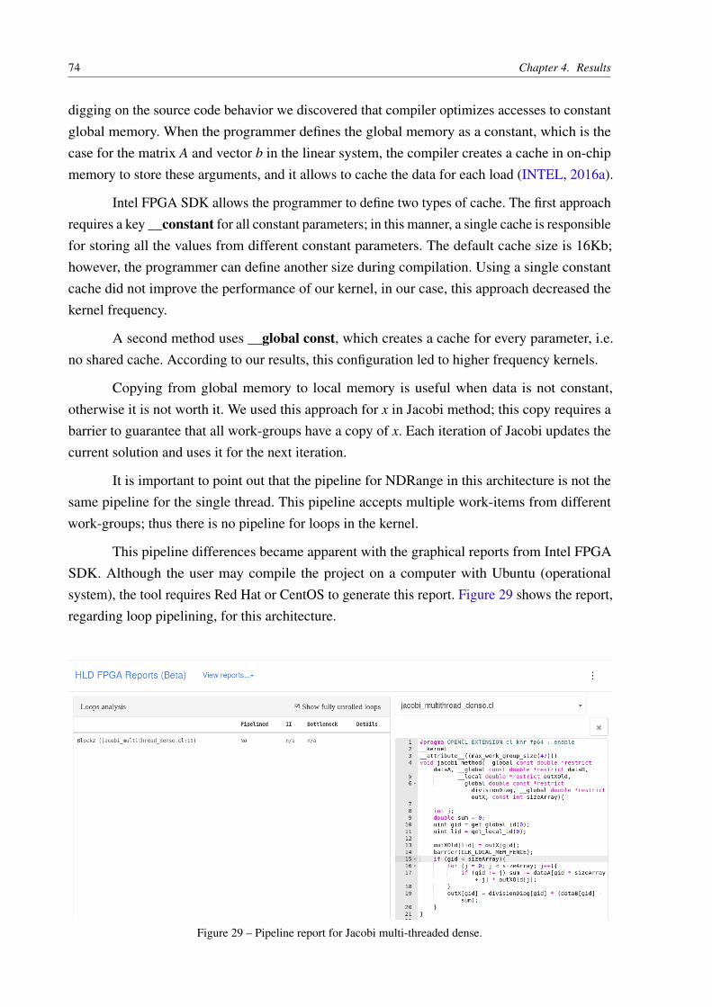
74 Chapter 4. Results
digging on the source code behavior we discovered that compiler optimizes accesses to constantglobal memory. When the programmer defines the global memory as a constant, which is thecase for the matrix A and vector b in the linear system, the compiler creates a cache in on-chipmemory to store these arguments, and it allows to cache the data for each load (INTEL, 2016a).
Intel FPGA SDK allows the programmer to define two types of cache. The first approachrequires a key __constant for all constant parameters; in this manner, a single cache is responsiblefor storing all the values from different constant parameters. The default cache size is 16Kb;however, the programmer can define another size during compilation. Using a single constantcache did not improve the performance of our kernel, in our case, this approach decreased thekernel frequency.
A second method uses __global const, which creates a cache for every parameter, i.e.no shared cache. According to our results, this configuration led to higher frequency kernels.
Copying from global memory to local memory is useful when data is not constant,otherwise it is not worth it. We used this approach for x in Jacobi method; this copy requires abarrier to guarantee that all work-groups have a copy of x. Each iteration of Jacobi updates thecurrent solution and uses it for the next iteration.
It is important to point out that the pipeline for NDRange in this architecture is not thesame pipeline for the single thread. This pipeline accepts multiple work-items from differentwork-groups; thus there is no pipeline for loops in the kernel.
This pipeline differences became apparent with the graphical reports from Intel FPGASDK. Although the user may compile the project on a computer with Ubuntu (operationalsystem), the tool requires Red Hat or CentOS to generate this report. Figure 29 shows the report,regarding loop pipelining, for this architecture.
Figure 29 – Pipeline report for Jacobi multi-threaded dense.
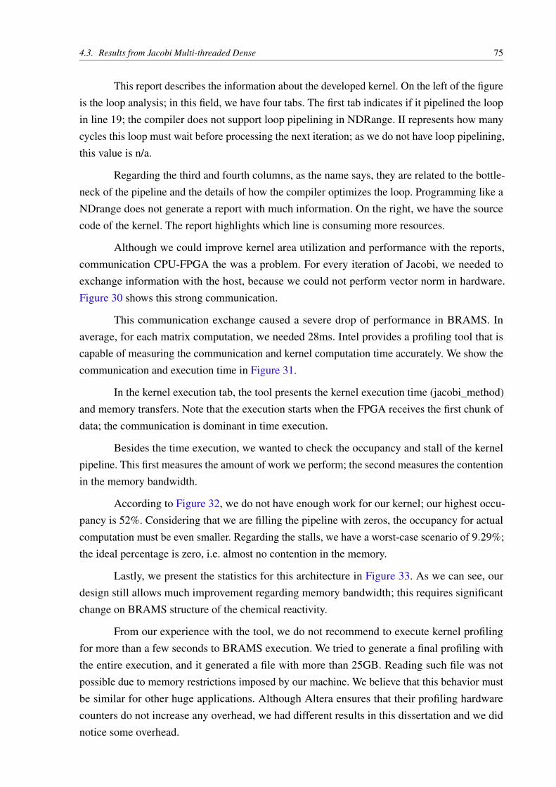
4.3. Results from Jacobi Multi-threaded Dense 75
This report describes the information about the developed kernel. On the left of the figureis the loop analysis; in this field, we have four tabs. The first tab indicates if it pipelined the loopin line 19; the compiler does not support loop pipelining in NDRange. II represents how manycycles this loop must wait before processing the next iteration; as we do not have loop pipelining,this value is n/a.
Regarding the third and fourth columns, as the name says, they are related to the bottle-neck of the pipeline and the details of how the compiler optimizes the loop. Programming like aNDrange does not generate a report with much information. On the right, we have the sourcecode of the kernel. The report highlights which line is consuming more resources.
Although we could improve kernel area utilization and performance with the reports,communication CPU-FPGA the was a problem. For every iteration of Jacobi, we needed toexchange information with the host, because we could not perform vector norm in hardware.Figure 30 shows this strong communication.
This communication exchange caused a severe drop of performance in BRAMS. Inaverage, for each matrix computation, we needed 28ms. Intel provides a profiling tool that iscapable of measuring the communication and kernel computation time accurately. We show thecommunication and execution time in Figure 31.
In the kernel execution tab, the tool presents the kernel execution time (jacobi_method)and memory transfers. Note that the execution starts when the FPGA receives the first chunk ofdata; the communication is dominant in time execution.
Besides the time execution, we wanted to check the occupancy and stall of the kernelpipeline. This first measures the amount of work we perform; the second measures the contentionin the memory bandwidth.
According to Figure 32, we do not have enough work for our kernel; our highest occu-pancy is 52%. Considering that we are filling the pipeline with zeros, the occupancy for actualcomputation must be even smaller. Regarding the stalls, we have a worst-case scenario of 9.29%;the ideal percentage is zero, i.e. almost no contention in the memory.
Lastly, we present the statistics for this architecture in Figure 33. As we can see, ourdesign still allows much improvement regarding memory bandwidth; this requires significantchange on BRAMS structure of the chemical reactivity.
From our experience with the tool, we do not recommend to execute kernel profilingfor more than a few seconds to BRAMS execution. We tried to generate a final profiling withthe entire execution, and it generated a file with more than 25GB. Reading such file was notpossible due to memory restrictions imposed by our machine. We believe that this behavior mustbe similar for other huge applications. Although Altera ensures that their profiling hardwarecounters do not increase any overhead, we had different results in this dissertation and we didnotice some overhead.

76 Chapter 4. Results
Load xjaj
(k)Load Sum
Pool of processing elements
a2a3⋯ a4am
a1
×
Load aj
+
Acc Sumj ← j + 1
Load bi
− Load 1/Aii
×
Store xi(k+1)
if (i ≠ j) ∧ (j < size)
j ← start
Single Compute Unit
i ← i + 1
i ← 1
Load xi(k-1)
−
+
Acc Conv
Load xi(k)
Square
i ← i + 1
SqrtConv
if Conv < 1e-7
Converged
it ← 1
it ← it + 1
if it < maxIt
if i < size
i ← 1
if i < size
CPU
CPU
Send Data
Receive Result andCompute norm
If ConvergedYes No
Figure 30 – CPU communicates with FPGA for every iteration. CPU sends to the FPGA the initial data, after FPGAprocessing it, the FPGA returns the result to the CPU, which in turn computes the vector norm anddecides if it sends another data or computes another iteration.
Despite the unsatisfactory performance of this architecture, we wanted to prove that ourdesign was correct. We measured the error in the Rosenbrock Method, this method computes alinear system, whose solution depends on Jacobi Method, and updates vector b for the next stage.After the fourth stage, the algorithm computes the error and rounding of the block. If rounding isover the tolerance, Rosenbrock updates each matrix A of the block. In this manner, a new set oflinear systems is available for each Rosenbrock stage.
Computing a 24-hour weather forecasting is not possible with this architecture due totime limitation. According to our extrapolation, it would be necessary 44 days to process thisresolution. So we measured just the first block of error of the Rosenbrock Method; we comparethe result with the first block of error in software using Sparse1.3a. We obtained a satisfactoryerror of 1.241371e−19.

4.3. Results from Jacobi Multi-threaded Dense 77
Figure 31 – Communication and execution time with Intel FPGA SDK profiling for kernels. Note that there is muchmore communication than computation.
Figure 32 – Efficiency of Jacobi multi-threaded dense with Intel FPGA SDK profiling for kernels. The red linepoints that the global memory reads (line 22) are the bottleneck of the application.
Figure 33 – Statistics of Jacobi multi-threaded dense with Intel FPGA SDK profiling for kernels.
Regarding energy consumption, we used PowerPlay Power Analyzer Tool from QuartusII; this tool is responsible for estimating the potency in mW of the circuit. According to the tool,our design consumes about 11W. We summarize the results of this architecture in Table 6 andTable 7. In the latter, we split the execution time from transfer time.
Table 6 – Results from Arch 1.
Area Frequency Time Energy Error19% 305 Mhz ∼44 days 11 W 1.241e-19

78 Chapter 4. Results
Table 7 – Timing results from Arch 1.
CPU-FPGA Execution FPGA-CPU Total Time11686us 9153us 7806us 28645us
4.4 Results from Jacobi Multi-threaded Sparse
In the profiling of the previous execution, we noted that communication was not the onlyproblem. We realized that there was extra computational time in the kernel; as we were using adense representation, we chose to avoid filling the pipeline with zeros.
We decided to use CSR, a sparse representation suitable for Sparse Matrix-Vectormultiplication (SpMV) (BELL; GARLAND, 2008). As we mentioned earlier, Jacobi methodis very similar to the matrix-vector algorithm; we used this characteristic in the choice of CSRformat.
In Figure 34, we show the statistics related to stall, occupancy, and bandwidth. Wecompare each result with the previous architecture, which is the most similar architecture. We donot present the loop pipeline report for this architecture (NDRange does not pipeline the loops).
Figure 34 – Efficiency of Jacobi multi-threaded sparse with Intel FPGA SDK profiling for kernels. Sparse formatcauses a severe drop of performance when saving the results back to the global memory.
The red rows represent the worst case in efficiency in the kernel. Reading from globalmemory is still the bottleneck of the application. We noted a severe drop in efficiency in savingthe results back to the global memory by using sparse format. We found two principal reasons forthis low efficiency: unbalanced access to global memory on the SpMV, and a higher percentageof stalls in the pipeline.
Regarding the stalls, in this architecture, the compiler could not hide global memorylatency due to the increase of three reads from the global memory. Although ia and ja are constantvectors, fetching from global memory must be avoided.
From Figure 35, we noted that changing matrix representation did not cause any im-provement in BRAMS execution. We decided to check kernel execution and memory transfers.
Again, we compare the results with the dense version. From this, we could find what wascausing the bad performance of Jacobi. Despite the lower execution time, we noted that therewere more memory transfers between computations than in Architecture 1 due to CSR format.

4.4. Results from Jacobi Multi-threaded Sparse 79
Figure 35 – Execution and memory transfer time of Jacobi multi-threaded sparse with Intel FPGA SDK profilingfor kernels. Note that transfer time did not improve due to variable sparsity of the matrices.
In the dense representation, we needed to transfer four data structures, and now we send six datastructures.
What draw our attention was the worst-case stall. In this version we improved in 6%. Asexpected, memory bandwidth is lower in the sparse architecture, since we need fewer data fromglobal memory. Figure 36 shows these statistics.
Figure 36 – Statistics of Jacobi multi-threaded sparse with Intel FPGA SDK profiling for kernels.
As we did in the previous architecture, we evaluated the precision from this architecture.We used the same set of configuration for comparison, i.e. we used extrapolation to measure theerror from the first block of the Rosenbrock Method obtained in Jacobi (hardware) comparedto the first block obtained in the Sparse1.3a (software). As expected, our average error is1.241371e−19; the same result from the previous architecture.
We also studied the impact of our new design on power consumption, as we mentionedearlier we cannot execute a weather forecasting for 24 hours due to time limitation. According toPowerPlay Power Analyzer Tool, this new architecture requires 14W. We show the summarizedresults in Table 8 and Table 9.

80 Chapter 4. Results
Table 8 – Results from Arch 2.
Area Frequency Time Energy Error29% 260 MHz ∼50 days 14 W 1.241e-19
Table 9 – Timing results from Arch 2.
CPU-FPGA Execution FPGA-CPU Total Time17597us 7846us 7863us 33306us
4.5 Results from Jacobi Single-threaded SparseThis architecture has a significant improvement over the previous ones. Now we can
compute the entire algorithm in hardware; this kernel is similar to a C to hardware.
We reused most of the knowledge of Architectures 1 and 2. At this point memoryhierarchy was a solid concept, and we used the best practices for a single thread kernel. Withthis new concept of programming, new problems arose; we discuss the problems, solutions, andresults from this architecture.
Our first version was a copy-paste of the Jacobi algorithm in software. We knew thatthere was room for plenty optimization, but we needed to perform the compilation to see theproblems. Intel FPGA SDK allows us to compile only the intermediate object file; this is muchfaster than generating the hardware.
Compiling the kernel source into an intermediate representation is enough to provide adetailed report of loop pipelining. As we mentioned earlier, a single thread kernel pipelines theiterations of the loops. We show this report in Figure 37 and discuss the improvements we made.
According to Figure 37, copy from the current to the previous solution has II of 1; thisthe most efficient pipeline, it means that every cycle computes an iteration. Traversing each lineof the matrix leads to a great result as well. We show an optimum pipeline in Figure 38.
This ideal pipeline is not present in the loop responsible for traversing each NNZ elementfrom the ith row. The problem with this loop is the data dependency on the sum accumulator; aswe cannot guarantee the same NNZ for each row, the pipeline must wait for the current iterationto finish before it starts the next one. This restriction also prevents us from using shift registerson the matrix-vector operation.
We show in Figure 39, how it is the pipeline for matrix-vector accumulator; we use twoiterations for simplicity. Note that this implies in an empty pipeline for some cycles, and it isresponsible for reducing the performance of Jacobi.
We have a similar problem in the convergence calculation, but now there is a well-formedloop. We declared an array (conv) to avoid data dependency, and we used a shift register toguarantee an optimum II. For using a shift register in OpenCL, we fully unrolled the loopresponsible for accumulating all the elements of conv. In Figure 40, we show the report for the

4.5. Results from Jacobi Single-threaded Sparse 81
Figure 37 – Pipeline report for Jacobi single-threaded sparse.

82 Chapter 4. Results
Cloc
k Cy
cles
I0
I1
I2
I3
I4
I5
0
1
2
3
4
5
6
7
Figure 38 – Optimum pipeline with II of 1, figure from Intel (2016a).Cl
ock
Cycle
s
I0
I1
0
1
2
3
4
5
6
7
8
9
10
11
12
13
Figure 39 – Matrix-vector pipeline with II of 11, based on Intel (2016a).
changes we made to this kernel.
These modification on the loop pipelines allowed us to reduce from 24 cycles to 14cycles; an improvement of 42% compared to the initial solution. During this optimization stage,we noted that our kernel demanded one global write for each iteration of Jacobi; we improvedthat by using a local memory and performing a single write in the end of computation. Withthis solution, we want to measure stall, occupancy, efficiency, execution and transfer time of thekernel. We profiled the kernel to obtain accurate measures.
In Figure 41 we show the kernel efficiency. Despite the lower occupancy ( 18%) comparedto the Architectures 1 and 2, we present optimum efficiency and stall for every pipeline. In thisarchitecture, there is no bottleneck, which means that we achieved the best pipeline configuration.The worst-case stall is still very close to zero.
Using a shift register for convergence calculation led to an effective bandwidth. The

4.5. Results from Jacobi Single-threaded Sparse 83
Figure 40 – Pipeline report for Jacobi single-threaded sparse optimized.

84 Chapter 4. Results
Figure 41 – Efficiency for Jacobi single-threaded sparse. After the modifications, all the pipelines shows 100% ofefficiency and almost zero stall.
same applies to the stalls in the pipeline; in the profiling, we can see numbers very close to zero.Besides the great results for the pipelines and stalls, we cannot infer the same about occupancy.
The changes in the architecture showed that occupancy is still a problem. That is nota design related problem, but a data problem. We do not provide enough data for the kernel,resulting in an idle time in the kernel; in future work, we intend to change BRAMS structurerelated to the chemical reactivity — spack data structure. In this manner, we will be able toimprove occupancy.
Even with low occupancy, we had an improvement with this design compared to theprevious ones. According to our results for a 24-hour weather forecasting, we improved thecomputational time in 63 times. We show in Figure 42 execution and memory transfers time.
Here we present an appropriate balance between execution and memory transfers. Thisresult relies on the improved Jacobi method; we implemented it 100% in hardware, in thismanner Jacobi only communicates with the host to receive and send data. According to ourmeasures, processing an entire linear system takes in average 1ms.
As we mentioned before, our design suffers from the lack of massive data to process.Figure 43 supports this affirmation by showing how much data is necessary during execution(measured column); in the same figure, we can see that the burst write is six times better in this

4.5. Results from Jacobi Single-threaded Sparse 85
Figure 42 – Execution and memory transfers time for Jacobi single-threaded sparse. Each bar in spjacobi_method1means a complete execution over a matrix.
architecture than in Architecture 2, and two times better than Architecture 1.
Figure 43 – Statistics for Jacobi single-threaded sparse.
Once we improved time execution, we could perform comparisons with software re-garding the precision of the floating point. For such comparison, we retrieved the first block oferror of the Rosenbrock Method in software and in hardware every timestep, then we measuredthe difference between the results. We measured the error for 1440 timesteps (24-hour weatherforecasting), and we obtained an average error of −6.277075e−09. If we compare in the sameconditions as the previous architectures, we obtain an average error of 8.027268e−20, i.e. 10×smaller than Architectures 1 and 2.
Jacobi impacts Rosenbrock convergence rate since it depends on the error of fourth stage.In the Literature, we find several works supporting that Jacobi method has a slow convergencerate (TAMULI et al., 2015; KHUSHPREETKAUR, 2012). We decided to take advantage of thisslow rate convergence to improve throughput by using double buffering scheme. In Figure 42,there are some matrices whose execution time is higher than memory transfer.
According to our experiments, we could not use double buffering on Intel FPGA SDKcorrectly. By using this scheme, we noted that data from different queues were overlapping the
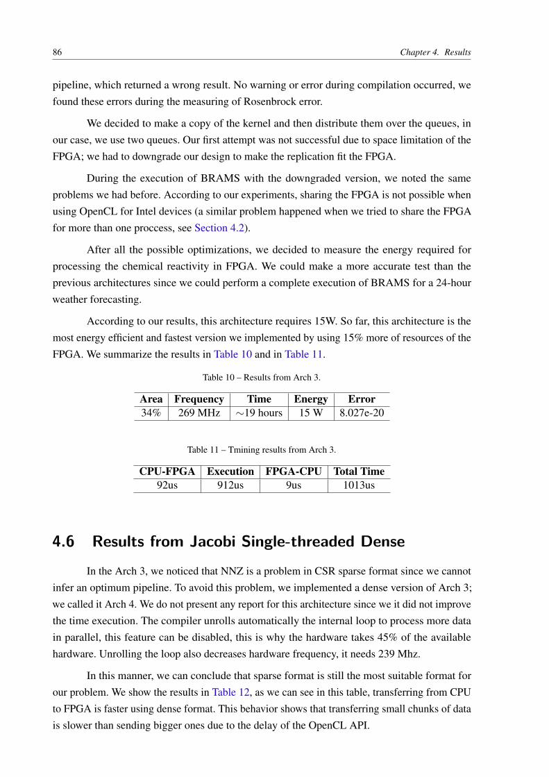
86 Chapter 4. Results
pipeline, which returned a wrong result. No warning or error during compilation occurred, wefound these errors during the measuring of Rosenbrock error.
We decided to make a copy of the kernel and then distribute them over the queues, inour case, we use two queues. Our first attempt was not successful due to space limitation of theFPGA; we had to downgrade our design to make the replication fit the FPGA.
During the execution of BRAMS with the downgraded version, we noted the sameproblems we had before. According to our experiments, sharing the FPGA is not possible whenusing OpenCL for Intel devices (a similar problem happened when we tried to share the FPGAfor more than one proccess, see Section 4.2).
After all the possible optimizations, we decided to measure the energy required forprocessing the chemical reactivity in FPGA. We could make a more accurate test than theprevious architectures since we could perform a complete execution of BRAMS for a 24-hourweather forecasting.
According to our results, this architecture requires 15W. So far, this architecture is themost energy efficient and fastest version we implemented by using 15% more of resources of theFPGA. We summarize the results in Table 10 and in Table 11.
Table 10 – Results from Arch 3.
Area Frequency Time Energy Error34% 269 MHz ∼19 hours 15 W 8.027e-20
Table 11 – Tmining results from Arch 3.
CPU-FPGA Execution FPGA-CPU Total Time92us 912us 9us 1013us
4.6 Results from Jacobi Single-threaded DenseIn the Arch 3, we noticed that NNZ is a problem in CSR sparse format since we cannot
infer an optimum pipeline. To avoid this problem, we implemented a dense version of Arch 3;we called it Arch 4. We do not present any report for this architecture since we it did not improvethe time execution. The compiler unrolls automatically the internal loop to process more datain parallel, this feature can be disabled, this is why the hardware takes 45% of the availablehardware. Unrolling the loop also decreases hardware frequency, it needs 239 Mhz.
In this manner, we can conclude that sparse format is still the most suitable format forour problem. We show the results in Table 12, as we can see in this table, transferring from CPUto FPGA is faster using dense format. This behavior shows that transferring small chunks of datais slower than sending bigger ones due to the delay of the OpenCL API.

4.7. Results from Sparse1.3a 87
Table 12 – Timing results from Arch 4.
CPU-FPGA Execution FPGA-CPU Total Time78us 3090us 16us 3184us
4.7 Results from Sparse1.3aWe also executed BRAMS with a single process with Sparse1.3a for a 24-hour weather
forecasting. We compare execution time from the software library with our Arch 3.
According to the results, the software versions takes about one hour and fifteen minutesto complete the execution. The same execution in hardware takes about 19 hours to execute, i.e.our hardware demands 15× more time execution, which is prohibitive in practice.
This poor execution time is related to several factors: (a) matrix size; (b) communication;and (c) one process per FPGA. Batched execution of linear algebra operations on small matricesare still a problem, and high performance accelerator remains a challenging problem (DONG et
al., 2016).
The focus of this project was to migrate a snippet of BRAMS to a heterogeneous machinewith FPGA, which was successfully performed. Time execution is not critical at this moment. InTable 13, we show the main characteristics of each implementation, and their advantages anddisadvantages. In Table 15, we compare the transfer and execution time for each architecture.
Table 13 – Table of comparison among implementations.
Features A B C D E Advantages DisadvantageArch 1 X X X Easy to understand and pro-
gram.Too much communicationbetween CPU-FPGA.
Arch 2 X X X Pipeline never computes ze-ros.
It is hard to define a suitableNDRange.
Arch 3 X X X 100% of Jacobi in hardware. Performance loss due to datarepresentation.
Arch 4 X X X No load imbalance. Performance loss comparedto Arch 3.
Sw X X X Fast and suitable for CPUs. It is not suitable for paral-lelism.
Features:
∙ A: Parallel algorithm;
∙ B: MPI Support;
∙ C: Coupled to BRAMS;
∙ D: Iterative method;
∙ E: Direct Method;
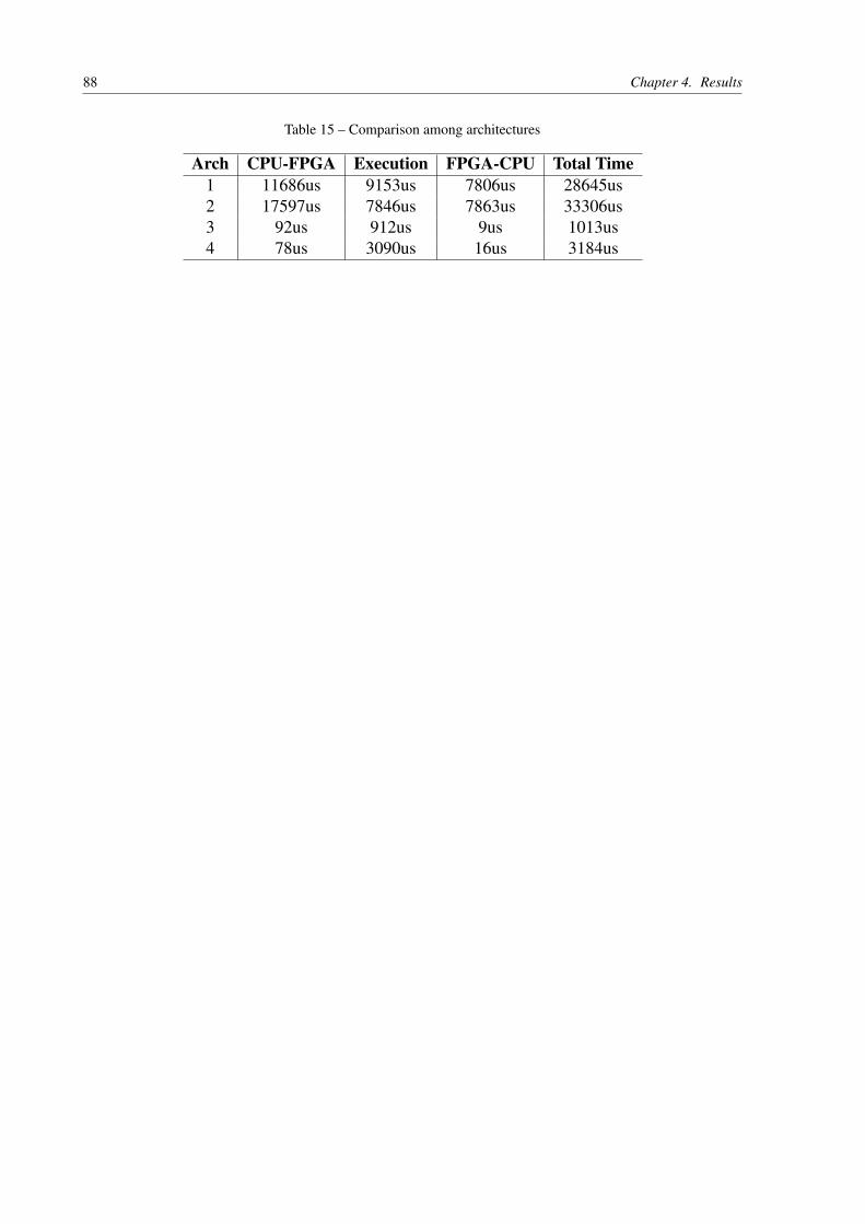
88 Chapter 4. Results
Table 15 – Comparison among architectures
Arch CPU-FPGA Execution FPGA-CPU Total Time1 11686us 9153us 7806us 28645us2 17597us 7846us 7863us 33306us3 92us 912us 9us 1013us4 78us 3090us 16us 3184us
89
CHAPTER
5CONCLUSION
In this project, we explore the possibility to use heterogeneous computing to solve thechem term. As we showed in the related works, coupling the chemical reactivity to BRAMS is acomplex task that we could perform by using OpenCL. We used this framework to implementthe dense and sparse version of Jacobi, an iterative linear solver.
We provide a parallel Jacobi suitable for FPGAs pipelining. By using FPGA, we couldimplement 100% of the algorithm on the device side and still maintain it coupled to BRAMS, tothe best of our knowledge, this is the first work that couples FPGA to BRAMS. According to ourtests, we proved the program presents the same behavior and accuracy of the software.
Such algorithm is critical to the solution of the chem term of the mass continuity equation;the chemical term became the most expensive when the developers included the gas chemicalmodule. We obtained the same results through profilings techniques applied to BRAMS, such asGprof. Currently, BRAMS executes only in CPU with MPI parallelism.
With this project, we could prove that porting parts of BRAMS to heterogeneous com-puting — CPU-FPGA — is possible. Our work allows the scientific community to explore moreparallel solution using FPGAs.
5.1 LimitationsAs we presented in Section 4.2, our design does not allow more than one process to
access the same device. The sparse format we chose imposes a severe drop of performance inpipeline execution. Performance is also a problem since our best architecture is 15× slower thansoftware.
CSR format imposes a load imbalance on the computation, and such problem imposesa higher latency in the pipeline. With this format, it is not possible to improve II of SpMVoperation since the sparsity of the matrices varies from 8% up to 25%.

90 Chapter 5. Conclusion
5.2 Future WorkIn future work, we intend to solve the limitations in our design. Our first target is the
Rosenbrock method, which we could perform the stages of the method in hardware, as we saw inFigure 2, all Rosenbrock stages require minor modifications and perform the same computation.Such implementation could be carried out if there is enough space in FPGA area.
We would also need to study the I/O involved in this process if this is a suitable solution.Regarding the sparse format, we could explore the viability of other sparse formats that couldperform in parallel. One of the options is the Ellpack format, which does not impose a loadimbalance. Although it seems a perfect solution, such format could lead to huge amount ofadditional memory and computation.
During BRAMS execution, we noted that much of the communication could be avoided.Instead of sending a single matrix to process and receiving a single result, we could process theentire block by sending all the data related to the block and manage them in hardware.
Another possible solution is to explore the serialization of the MPI processes, i.e. whenthey reach FPGA execution only one of the process could perform the computation at a time. Forthis, we could use a master-slave approach similar to what already happens in BRAMS, wherejust the master has access to the device.
A harder optimization requires the modification of BRAMS source code related tochemical reactivity data structure — spack data structure. Fortran90 does not align componentsof derived type, i.e. components from the data structure. A deeper study of this structure couldboost BRAMS performance.
91
BIBLIOGRAPHY
ACCELEWARE. OpenCL on FPGAs for GPU Programmers. [S.l.], 2014. Available at:<https://www.ece.cmu.edu/~calcm/carl/lib/exe/fetch.php?media=carl15-gupta.pdf>. Accessedon: May 12, 2017. Cited on page 52.
ACKERMAN, P.; ACKERMAN, S.; KNOX, J. Meteorology. Jones & Bartlett Learning,LLC, 2013. ISBN 9781284027389. Available at: <https://books.google.com.br/books?id=qWcrAQAAQBAJ>. Cited on page 30.
AHMAD, S.; BOPPANA, V.; GANUSOV, I.; KATHAIL, V.; RAJAGOPALAN, V.; WITTIG, R.A 16-nm multiprocessing system-on-chip field-programmable gate array platform. IEEE Micro,IEEE, v. 36, n. 2, p. 48–62, 2016. Cited 2 times on pages 13 and 45.
ALISSON, E. Sistema faz previsões simultâneas de tempo e qualidade do ar na Américado Sul. [S.l.], 2016. Available at: <http://agencia.fapesp.br/sistema_faz_previsoes_simultaneas_de_tempo_e_qualidade_do_ar_na_america_do_sul/22921/>. Accessed on: Mar 20, 2017. Citedon page 55.
ALTERA. Implementing FPGA Design with the OpenCL Standard. [S.l.], 2013. Availableat: <https://www.altera.com/en_US/pdfs/literature/wp/wp-01173-opencl.pdf>. Accessed on:May 4, 2017. Cited 2 times on pages 13 and 42.
AN, J.; WANG, D. Efficient one-sided jacobi svd computation on amd gpu using opencl. In:2016 IEEE 13th International Conference on Signal Processing (ICSP). [S.l.: s.n.], 2016. p.491–495. ISSN 2164-5221. Cited on page 51.
ANTON, H.; RORRES, C. Elementary Linear Algebra: Applications Version, 11th Edition:.Wiley Global Education, 2013. ISBN 9781118879160. Available at: <https://books.google.com.br/books?id=loRbAgAAQBAJ>. Cited on page 35.
BELL, N.; GARLAND, M. Efficient sparse matrix-vector multiplication on CUDA. [S.l.],2008. Cited on page 78.
BINDEL, D.; GOODMAN, J. Principles of scientific computing linear algebra ii, algorithms.2006. Cited on page 36.
BITTWARE, I. S5-PCIe-HQ. [S.l.], 2015. 57 p. Cited 2 times on pages 13 and 46.
BLICKLE, T.; TEICH, J.; THIELE, L. System-level synthesis using evolutionary algorithms.Design Automation for Embedded Systems, Springer, v. 3, n. 1, p. 23–58, 1998. Cited onpage 48.
BOBDA, C. Introduction to Reconfigurable Computing: Architectures, Algorithms, andApplications. Springer Netherlands, 2007. ISBN 9781402061004. Available at: <https://books.google.com.br/books?id=\_cNSgjR32LkC>. Cited on page 44.
BORKAR, S.; CHIEN, A. A. The future of microprocessors. Communications of the ACM,ACM, v. 54, n. 5, p. 67–77, 2011. Cited on page 28.
92 Bibliography
BOUT, D. V. FPGAs?! Now What? [s.n.], 2011. Available at: <http://www.xess.com/static/media/appnotes/FpgasNowWhatBook.pdf>. Cited on page 45.
BRAVO, I.; JIMENEZ, P.; MAZO, M.; LAZARO, J. L.; GARDEL, A. Implementation in fpgasof jacobi method to solve the eigenvalue and eigenvector problem. In: 2006 InternationalConference on Field Programmable Logic and Applications. [S.l.: s.n.], 2006. p. 1–4. ISSN1946-147X. Cited on page 49.
BUCHTY, R.; HEUVELINE, V.; KARL, W.; WEISS, J.-P. A survey on hardware-aware andheterogeneous computing on multicore processors and accelerators. Concurrency and Compu-tation: Practice and Experience, Wiley Online Library, v. 24, n. 7, p. 663–675, 2012. Citedon page 38.
CHE, S.; LI, J.; SHEAFFER, J. W.; SKADRON, K.; LACH, J. Accelerating compute-intensiveapplications with gpus and fpgas. In: IEEE. Application Specific Processors, 2008. SASP 2008.Symposium on. [S.l.], 2008. p. 101–107. Cited on page 28.
CHENG, J.; GROSSMAN, M.; MCKERCHER, T. Professional CUDA C Programming.Wiley, 2014. (Wrox : Programmer to Programmer). ISBN 9781118739310. Available at:<https://books.google.com.br/books?id=Jgx\_BAAAQBAJ>. Cited on page 67.
CHU, P. FPGA Prototyping by VHDL Examples: Xilinx Spartan-3 Version. Wi-ley, 2011. ISBN 9781118210604. Available at: <https://books.google.com.br/books?id=nXdbDRUUCyUC>. Cited on page 44.
CONG, J.; ZOU, Y. Fpga-based hardware acceleration of lithographic aerial image simulation.ACM Transactions on Reconfigurable Technology and Systems (TRETS), ACM, v. 2, n. 3,p. 17, 2009. Cited on page 28.
CRASSIER, V.; SUHRE, K.; TULET, P.; ROSSET, R. Development of a reduced chemicalscheme for use in mesoscale meteorological models. Atmospheric Environment, Elsevier,v. 34, n. 16, p. 2633–2644, 2000. Cited on page 31.
CZAJKOWSKI, T. S.; AYDONAT, U.; DENISENKO, D.; FREEMAN, J.; KINSNER, M.;NETO, D.; WONG, J.; YIANNACOURAS, P.; SINGH, D. P. From opencl to high-performancehardware on fpgas. In: IEEE. Field Programmable Logic and Applications (FPL), 2012 22ndInternational Conference on. [S.l.], 2012. p. 531–534. Cited on page 41.
CZAJKOWSKI, T. S.; NETO, D.; KINSNER, M.; AYDONAT, U.; WONG, J.; DENISENKO, D.;YIANNACOURAS, P.; FREEMAN, J.; SINGH, D. P.; BROWN, S. D. Opencl for fpgas: Proto-typing a compiler. In: Int’l Conf. on Engineering of Reconfigurable Systems and Algorithms(ERSA). [S.l.: s.n.], 2012. p. 3–12. Cited 3 times on pages 13, 43, and 44.
DAGA, V.; GOVINDU, G.; PRASANNA, V.; GANGADHARAPALLI, S.; SRIDHAR, V. Ef-ficient floating-point based block lu decomposition on fpgas. In: International Conferenceon Engineering of Reconfigurable Systems and Algorithms, Las Vegas. [S.l.: s.n.], 2004. p.21–24. Cited on page 49.
DAVISON, M. Shallow/Deep Convection. [S.l.], 1999. Available at: <http://origin.wpc.ncep.noaa.gov/international/training/deep/sld001.htm>. Accessed on: May 8, 2017. Cited on page30.

Bibliography 93
DINIGROUP. FPGA Selection Guide. [S.l.], 2017. Available at: <http://www.dinigroup.com/product/common/DINI_selection_guide_v540.pdf>. Accessed on: May 4, 2017. Cited on page46.
DONG, T.; HAIDAR, A.; LUSZCZEK, P.; TOMOV, S.; ABDELFATTAH, A.; DONGARRA, J.Magma batched: A batched blas approach for small matrix factorizations and applications ongpus. Aug 2016. Cited on page 87.
ELLER, P.; SINGH, K.; SANDU, A. Development and acceleration of parallel chemical transportmodels. In: SOCIETY FOR COMPUTER SIMULATION INTERNATIONAL. Proceedings ofthe 2010 Spring Simulation Multiconference. [S.l.], 2010. p. 90. Cited 2 times on pages 49and 52.
ERNST, R.; HENKEL, J.; BENNER, T. Hardware-software cosynthesis for microcontrollers.IEEE Design Test of Computers, v. 10, n. 4, p. 64–75, Dec 1993. ISSN 0740-7475. Cited onpage 48.
FAZENDA, A. L.; ENARI, E. H.; RODRIGUES, L. F.; PANETTA, J. Towards production codeeffective portability among vector machines and microprocessor-based architectures. In: IEEE.Computer Architecture and High Performance Computing, 2006. SBAC-PAD’06. 18THInternational Symposium on. [S.l.], 2006. p. 11–20. Cited on page 51.
FAZENDA, A. L.; RODRIGUES, E. R.; TOMITA, S. S.; PANETTA, J.; MENDES, C. L.Improving the scalability of an operational scientific application in a large multi-core cluster. In:2012 13th Symposium on Computer Systems. [S.l.: s.n.], 2012. p. 126–132. Cited on page34.
FERNANDES, A. d. A. Paralelização do Termo de Reatividade Química do Modelo Am-biental CCATT-BRAMS utilizando um Solver Baseado em Estimação Linear Ótima. 76 p.Dissertação (Mestrado) — Instituto Nacional de Pesquisas Espaciais, 2014. Master’s thesis atINPE-SP. Cited 4 times on pages 31, 51, 55, and 62.
FOERTSCH, J.; JOHNSON, J.; NAGVAJARA, P. Jacobi load flow accelerator using fpga. In:Proceedings of the 37th Annual North American Power Symposium, 2005. [S.l.: s.n.], 2005.p. 448–454. Cited on page 49.
FREITAS, S.; LONGO, K.; DIAS, M. S.; CHATFIELD, R.; DIAS, P. S.; ARTAXO, P.; AN-DREAE, M.; GRELL, G.; RODRIGUES, L.; FAZENDA, A. et al. The coupled aerosol and tracertransport model to the brazilian developments on the regional atmospheric modeling system(catt-brams)–part 1: Model description and evaluation. Atmospheric Chemistry and Physics,Copernicus GmbH, v. 9, n. 8, p. 2843–2861, 2009. Cited on page 29.
FREITAS, S.; LONGO, K.; TRENTMANN, J.; LATHAM, D. Technical note: Sensitivity of 1-dsmoke plume rise models to the inclusion of environmental wind drag. Atmospheric Chemistryand Physics, Copernicus GmbH, v. 10, n. 2, p. 585–594, 2010. Cited on page 30.
FU, H.; GAN, L.; YANG, C.; XUE, W.; WANG, L.; WANG, X.; HUANG, X.; YANG, G. Solvingglobal shallow water equations on heterogeneous supercomputers. PloS one, Public Library ofScience, v. 12, n. 3, p. e0172583, 2017. Cited on page 52.
GAILLY, J.-l.; ADLER, M. A Massively Spiffy Yet Delicately Unobtrusive CompressionLibrary (Also Free, Not to Mention Unencumbered by Patents). [S.l.], 2015. Available at:<http://www.zlib.net/>. Accessed on: Dec. 15, 2015. Cited on page 34.

94 Bibliography
GALLERY, R. Hardware/software codesign. The ITB Journal, v. 4, n. 1, p. 5, 2015. Cited 2times on pages 46 and 47.
GOLUB, G.; LOAN, C. V. Matrix Computations. Johns Hopkins University Press, 2013.(Johns Hopkins Studies in the Mathematical Sciences). ISBN 9781421407944. Available at:<https://books.google.com.br/books?id=X5YfsuCWpxMC>. Cited on page 36.
GOMES, G. A. A. Linear solvers for stable fluids: Gpu vs cpu. 17th EncontroPortugues deComputacaoGrafica (EPCG09), p. 145–153, 2009. Cited on page 51.
GRAHAM, S.; PARKINSON, C.; CHAHINE, M. Weather Forecasting Through the Ages.[S.l.], 2002. Available at: <http://earthobservatory.nasa.gov/Features/WxForecasting/wx.php>.Accessed on: July 30, 2015. Cited on page 25.
GRØNØS, S. Vilhelm bjerknes’ vision for scientific weather prediction. The Nordic Seas: AnIntegrated Perspective, Wiley Online Library, p. 357–366, 2005. Cited on page 26.
GROPP, W.; HOEFLER, T.; LUSK, E.; THAKUR, R. Using Advanced MPI: Modern Featuresof the Message-Passing Interface. MIT Press, 2014. (Computer science & intelligent systems).ISBN 9780262527637. Available at: <https://books.google.com.br/books?id=Po5IBQAAQBAJ>.Cited on page 35.
GROUP, H. HDF5 Technologies. [S.l.], 2011. Available at: <https://www.hdfgroup.org/about/hdf_technologies.html>. Accessed on: Dec. 15, 2015. Cited on page 34.
GUPTA, P. Xeon+FPGA Platform for the Data Center. [S.l.], 2015. Available at: <https://www.ece.cmu.edu/~calcm/carl/lib/exe/fetch.php?media=carl15-gupta.pdf>. Accessed on: Apr10, 2017. Cited on page 46.
GUPTA, R. K.; MICHELI, G. D. Hardware-software cosynthesis for digital systems. IEEEDesign Test of Computers, v. 10, n. 3, p. 29–41, Sept 1993. ISSN 0740-7475. Cited on page48.
GáCITA, M. S. Estudos Numéricos de Química Atmosférica para a região do Caribe eAmérica Central com Ênfase em Cuba. Dissertação (Mestrado) — Instituto Nacional dePesquisas Espaciais - INPE, São José dos Campos - SP - Brasil, 2011. Cited on page 31.
HARRIS, M. How to Optimize Data Transfers in CUDA C/C++. [S.l.], 2012. Available at:<https://devblogs.nvidia.com/parallelforall/how-optimize-data-transfers-cuda-cc/>. Accessedon: Apr 3, 2017. Cited 2 times on pages 14 and 67.
HENKEL, M. 21st Century Homestead: Sustainable Agriculture II: Farming and NaturalResources. Lulu.com, 2015. ISBN 9781312939684. Available at: <https://books.google.com.br/books?id=jmHxCQAAQBAJ>. Cited on page 25.
HRZ. MPI + OpenCL Altera. [S.l.], 2017. Available at: <http://www.alteraforum.com/forum/showthread.php?t=55035>. Accessed on: Mar 6, 2017. Cited on page 71.
INPE/CPTEC. Model Description. [S.l.], 2015. Available at: <http://brams.cptec.inpe.br/>.Accessed on: Dec. 16, 2015. Cited on page 29.
INTEL. Intel FPGA SDK for OpenCL – Best Practices Guide. [S.l.], 2016. Avail-able at: <https://www.altera.com/en_US/pdfs/literature/hb/opencl-sdk/aocl-best-practices-guide.pdf>. Accessed on: Mar 29, 2017. Cited 8 times on pages 13, 15, 42, 43, 57, 64, 74, and 82.

Bibliography 95
. Intel FPGA SDK for OpenCL – Programming Guide. [S.l.], 2016. Avail-able at: <https://www.altera.com/en_US/pdfs/literature/hb/opencl-sdk/aocl_programming_guide.pdf>. Accessed on: May 4, 2017. Cited on page 42.
JANIK, I.; TANG, Q.; KHALID, M. An overview of altera sdk for opencl: A user perspec-tive. In: IEEE. Electrical and Computer Engineering (CCECE), 2015 IEEE 28th CanadianConference on. [S.l.], 2015. p. 559–564. Cited 2 times on pages 43 and 44.
KAPRE, N.; DEHON, A. Parallelizing sparse matrix solve for spice circuit simulation using fpgas.In: IEEE. Field-Programmable Technology, 2009. FPT 2009. International Conference on.[S.l.], 2009. p. 190–198. Cited on page 48.
. rmSPICE2: Spatial processors interconnected for concurrent execution for acceleratingthe spice circuit simulator using an fpga. IEEE Transactions on Computer-Aided Design ofIntegrated Circuits and Systems, v. 31, n. 1, p. 9–22, Jan 2012. ISSN 0278-0070. Cited onpage 49.
KARNIADAKIS, G.; KIRBY, R. Parallel Scientific Computing in C++ and MPI: A Seam-less Approach to Parallel Algorithms and their Implementation. Cambridge UniversityPress, 2003. ISBN 9781107494770. Available at: <https://books.google.com.br/books?id=Py8XAgAAQBAJ>. Cited on page 35.
KASBAH, S. J.; DAMAJ, I. W. The jacobi method in reconfigurable hardware. In: WorldCongress on Engineering. [S.l.: s.n.], 2007. p. 823–827. Cited on page 49.
KHUSHPREETKAUR, H. Convergence of jacobi and gauss-seidel method and error reductionfactor. IOSR Journal of Mathematics (IOSRJM), v. 2, p. 20–23, 2012. Cited on page 85.
KIRK, D. B.; WEN-MEI, W. H. Programming massively parallel processors: a hands-onapproach. [S.l.]: Newnes, 2012. Cited on page 27.
KRISHNAIYER, R. Data Alignment to Assist Vectorization. [S.l.], 2015. Available at: <https://software.intel.com/en-us/articles/data-alignment-to-assist-vectorization>. Accessed on: Mar21, 2017. Cited on page 62.
KUNDERT, K. S.; SANGIOVANNI-VINCENTELLI, A. Sparse1.3. [S.l.], 1988. Available at:<http://web.cs.ucla.edu/classes/CS258G/sis-1.3/sis/linsolv/>. Accessed on: Oct. 28, 2015. Cited2 times on pages 32 and 36.
LABORATORY, E. S. R. Regional Modeling. [S.l.], 2015. Available at: <http://www.esrl.noaa.gov/research/themes/regional>. Accessed on: July 30, 2015. Cited 2 times on pages 25 and 26.
LAMBERS, J. Jacobi Methods. [S.l.], 2010. Available at: <http://web.stanford.edu/class/cme335/lecture7.pdf>. Accessed on: May 11, 2017. Cited on page 51.
LARSON, R. Elementary Linear Algebra. Cengage Learning, 2016. ISBN 9781305887824.Available at: <https://books.google.com.br/books?id=2sQaCgAAQBAJ>. Cited on page 35.
LINFORD, J. C.; MICHALAKES, J.; VACHHARAJANI, M.; SANDU, A. Multi-core ac-celeration of chemical kinetics for simulation and prediction. In: IEEE. High PerformanceComputing Networking, Storage and Analysis, Proceedings of the Conference on. [S.l.],2009. p. 1–11. Cited on page 55.
96 Bibliography
LINFORD, J. C.; SANDU, A. Vector stream processing for effective application of heterogeneousparallelism. In: Proceedings of the 2009 ACM Symposium on Applied Computing. NewYork, NY, USA: ACM, 2009. (SAC ’09), p. 976–980. ISBN 978-1-60558-166-8. Available at:<http://doi.acm.org/10.1145/1529282.1529496>. Cited on page 51.
LONGO, K.; FREITAS, S.; PIRRE, M.; MARÉCAL, V.; RODRIGUES, L.; PANETTA, J.;ALONSO, M.; ROSÁRIO, N.; MOREIRA, D.; GÁCITA, M. et al. The chemistry catt–bramsmodel (ccatt–brams 4.5): a regional atmospheric model system for integrated air quality andweather forecasting and research. Model Dev. Discuss, v. 6, p. 1173–1222, 2013. Cited 4 timeson pages 13, 29, 30, and 31.
LYNCH, P. The origins of computer weather prediction and climate modeling. Journal ofComputational Physics, Elsevier, v. 227, n. 7, p. 3431–3444, 2008. Cited on page 26.
MCEWEN, J.; EYERS, D. szip1.0b1 Data compression on the sphere. [S.l.], 2011. Availableat: <http://www.jasonmcewen.org/codes/szip/>. Accessed on: Dec. 15, 2015. Cited on page 34.
MICHALAKES, J.; VACHHRAJANI, M. Gpu acceleration of numerical weather predic-tion. Parallel Processing Letters, v. 18, n. 04, p. 531–548, 2008. Available at: <http://www.worldscientific.com/doi/abs/10.1142/S0129626408003557>. Cited on page 51.
MOORE ANDREW; WILSON, R. FPGAs for Dummies. Wiley, 2017. ISBN 978-1-119-39047-3. Available at: <https://www.altera.com/content/dam/altera-www/global/en_US/pdfs/literature/misc/fpgas_for_dummies_ebook.pdf>. Cited on page 44.
MOREIRA, D.; FREITAS, S.; BONATTI, J.; MERCADO, L.; ROSÁRIO, N.; LONGO, K.;MILLER, J.; GLOOR, M.; GATTI, L. Coupling between the jules land-surface scheme andthe ccatt-brams atmospheric chemistry model (jules-ccatt-brams1. 0): applications to numericalweather forecasting and the co 2 budget in south america. Geoscientific Model Development,Copernicus GmbH, v. 6, n. 4, p. 1243–1259, 2013. Cited on page 32.
MORRIS, G. R.; PRASANNA, V. K. An fpga-based floating-point jacobi iterative solver. In:IEEE. Parallel Architectures, Algorithms and Networks, 2005. ISPAN 2005. Proceedings.8th International Symposium on. [S.l.], 2005. p. 8–pp. Cited 3 times on pages 36, 49, and 57.
MPICH. MPICH Overview. [S.l.], 2015. Available at: <https://www.mpich.org/about/overview/>. Accessed on: Dec. 15, 2015. Cited on page 34.
MUNSHI, A. The OpenCL Specification. [S.l.], 2009. Available at: <https://www.khronos.org/registry/OpenCL/specs/opencl-1.0.pdf>. Accessed on: Mar 21, 2017. Cited 4 times on pages13, 40, 41, and 60.
MUNSHI, A.; GASTER, B.; MATTSON, T. G.; GINSBURG, D. OpenCL programming guide.[S.l.]: Pearson Education, 2011. Cited 4 times on pages 37, 38, 40, and 61.
NIELSEN, F. Introduction to HPC with MPI for Data Science. Springer International Pub-lishing, 2016. (Undergraduate Topics in Computer Science). ISBN 9783319219035. Availableat: <https://books.google.com.br/books?id=eDiFCwAAQBAJ>. Cited on page 35.
OSTHOFF, C.; SCHEPKE, C.; VILASBÔAS, F.; BOITO, F.; PANETTA, J.; PILLA, L.; MAIL-LARD, N.; GRUNMANN, P.; DIAS, P. L. S.; LOPES, P. P. et al. Improving AtmosphericModel Performance on a Multi-Core Cluster System. [S.l.]: INTECH Open Access Publisher,2012. Cited on page 26.

Bibliography 97
PANETTA, J. Production. [S.l.], 2015. Available at: <http://www.cesup.ufrgs.br/videos/jairo-panetta/view>. Accessed on: Oct. 28, 2015. Cited on page 26.
PATTERSON, D.; HENNESSY, J. Computer Organization and Design: The Hardware/soft-ware Interface. Morgan Kaufmann, 2012. (Morgan Kaufmann Series in Computer Graphics).ISBN 9780123747501. Available at: <https://books.google.com.br/books?id=DMxe9AI4-9gC>.Cited 3 times on pages 13, 37, and 38.
PENG, R. Algorithm design using spectral graph theory. Tese (Doutorado) — MicrosoftResearch, 2013. Cited on page 36.
PRASANNA, V. K.; MORRIS, G. R. Sparse matrix computations on reconfigurable hardware.Computer, v. 40, n. 3, p. 58–64, March 2007. ISSN 0018-9162. Cited on page 49.
RANDALL, D. A. An Introduction to Atmospheric Modeling. [s.n.], 2013. Available at:<http://kiwi.atmos.colostate.edu/group/dave/at604.html>. Cited on page 30.
RAYMOND, E. S. The Cathedral & the Bazaar: Musings on linux and open source by anaccidental revolutionary. [S.l.]: " O’Reilly Media, Inc.", 2001. Cited on page 29.
REW, R.; DAVIS, G. Netcdf: an interface for scientific data access. IEEE Computer Graphicsand Applications, v. 10, n. 4, p. 76–82, July 1990. ISSN 0272-1716. Cited on page 32.
REW, R. K. What Is netCDF? [S.l.], 2015. Available at: <http://www.unidata.ucar.edu/software/netcdf/docs/faq.html#whatisit>. Accessed on: Dec. 15, 2015. Cited on page 32.
RODRIGUES, E. R.; MADRUGA, F. L.; NAVAUX, P. O.; PANETTA, J. Multi-core awareprocess mapping and its impact on communication overhead of parallel applications. In: IEEE.Computers and Communications, 2009. ISCC 2009. IEEE Symposium on. [S.l.], 2009. p.811–817. Cited on page 57.
RUAN, H.; HUANG, X.; FU, H.; YANG, G. Jacobi solver: A fast fpga-based engine system forjacobi method. Research Journal of Applied Sciences, Engineering and Technology, March2013. ISSN 2040-7459. Cited on page 50.
SCHAUMONT, P. A practical introduction to hardware/software codesign. [S.l.]: SpringerScience & Business Media, 2012. Cited 3 times on pages 13, 47, and 48.
SCHMID, M.; REICHE, O.; SCHMITT, C.; HANNIG, F.; TEICH, J. Code generation forhigh-level synthesis of multiresolution applications on fpgas. arXiv preprint arXiv:1408.4721,2014. Cited 2 times on pages 50 and 51.
SILVA, E. Pereira da. Projeto de um Processador Open Source em Bluespec Baseado no Pro-cessador Soft-core Nios II da Altera. 95 p. Dissertação (Mestrado em Ciência da Computação)— Univerisity of São Paulo, São Paulo, 2014. Cited on page 45.
SOCIETY, A. M. Weather Forecasting. [S.l.], 2015. Available at: <http://www.ametsoc.org/policy/weaforc.html>. Accessed on: Sept. 27, 2015. Cited on page 25.
STOCKWELL, W. R.; KIRCHNER, F.; KUHN, M.; SEEFELD, S. A new mechanism forregional atmospheric chemistry modeling. Journal of Geophysical Research: Atmospheres(1984–2012), Wiley Online Library, v. 102, n. D22, p. 25847–25879, 1997. Cited on page 31.

98 Bibliography
TAMULI, M.; DEBNATH, S.; RAY, A.; MAJUMDER, S. A review on jacobi iterative solver andits hardware based performance analysis. In: proceedings of 1st International Conference onPower, Dielectric and Energy Management at NERIST. [S.l.: s.n.], 2015. p. 10–11. Citedon page 85.
TEICH, J. Hardware/software codesign: The past, the present, and predicting the future. Pro-ceedings of the IEEE, IEEE, v. 100, n. Special Centennial Issue, p. 1411–1430, 2012. Citedon page 46.
TSUCHIYAMA, R.; NAKAMURA, T.; IIZUKA, T.; ASAHARA, A.; SON, J.; MIKI, S. TheOpenCL Programming Book. Fixstars, 2012. Available at: <https://books.google.com.br/books?id=O86m1hJxA6QC>. Cited 2 times on pages 37 and 40.
VAUGHAN, C. Deep Thoughts on Deep Convection. [S.l.], 2009. Available at: <http://blogs.ei.columbia.edu/2009/03/01/deep-thoughts-on-deep-convection/>. Accessed on: May 8, 2017.Cited on page 30.
VERWER, J. G.; SPEE, E. J.; BLOM, J. G.; HUNDSDORFER, W. A second-order rosen-brock method applied to photochemical dispersion problems. SIAM Journal on ScientificComputing, SIAM, v. 20, n. 4, p. 1456–1480, 1999. Cited on page 31.
WANG, T.; WEI, P. Hardware efficient architectures of improved jacobi method to solve the eigenproblem. In: 2010 2nd International Conference on Computer Engineering and Technology.[S.l.: s.n.], 2010. v. 6, p. V6–22–V6–25. Cited on page 49.
WANNER, G.; HAIRER, E. Solving ordinary differential equations ii. Stiff and Differential-Algebraic Problems, 1991. Cited on page 31.
WARNER, T. T. Numerical weather and climate prediction. [S.l.]: Cambridge UniversityPress, 2010. Cited 2 times on pages 25 and 26.
WILLIS, E. P.; HOOKE, W. H. Cleveland abbe and american meteorology, 1871-1901. Bulletinof the American Meteorological Society, v. 87, n. 3, p. 315–326, 2006. Cited on page 26.
WU, W.; SHAN, Y.; CHEN, X.; WANG, Y.; YANG, H. Fpga accelerated parallel sparse matrixfactorization for circuit simulations. In: SPRINGER. International Symposium on AppliedReconfigurable Computing. [S.l.], 2011. p. 302–315. Cited on page 49.
YANG, C.; XUE, W.; FU, H.; YOU, H.; WANG, X.; AO, Y.; LIU, F.; GAN, L.; XU, P.; WANG, L.et al. 10m-core scalable fully-implicit solver for nonhydrostatic atmospheric dynamics. In: IEEEPRESS. Proceedings of the International Conference for High Performance Computing,Networking, Storage and Analysis. [S.l.], 2016. p. 6. Cited on page 52.
YARWOOD, G.; RAO, S.; YOCKE, M.; WHITTEN, G. Updates to the carbon bond chemicalmechanism: Cb05. Final report to the US EPA, RT-0400675, v. 8, 2005. Cited on page 31.
ZHANG, H.; LINFORD, J. C.; SANDU, A.; SANDER, R. Chemical mechanism solvers inair quality models. Atmosphere, v. 2, n. 3, p. 510–532, 2011. ISSN 2073-4433. Available at:<http://www.mdpi.com/2073-4433/2/3/510>. Cited 2 times on pages 55 and 57.
ZHUO, L.; PRASANNA, V. K. Sparse matrix-vector multiplication on fpgas. In: Proceedingsof the 2005 ACM/SIGDA 13th International Symposium on Field-programmable Gate Ar-rays. New York, NY, USA: ACM, 2005. (FPGA ’05), p. 63–74. ISBN 1-59593-029-9. Availableat: <http://doi.acm.org/10.1145/1046192.1046202>. Cited on page 48.

Bibliography 99
. High-performance and parameterized matrix factorization on fpgas. In: IEEE. FieldProgrammable Logic and Applications, 2006. FPL’06. International Conference on. [S.l.],2006. p. 1–6. Cited on page 49.


Appendix

103
APPENDIX
AINSTALLATION
In this Appendix, we describe the installation of BRAMS 5.2 and its libraries. Beforecompiling BRAMS and the necessary libraries, the user needs to install Intel Fortran Compiler1
(ifort); our tests with gfortran failed.
After installing ifort, the user can proceed to compile the libraries2 below. We provideuseful links to libraries and BRAMS source code in Annex A.
∙ netcdf 4.1.3;
∙ hdf5 1.8.15;
∙ zlib 1.2.8;
∙ szip 2.1;
∙ mpich 3.1.4.
In this section, we consider the following directory structure for local installation3.
Main directory: home/<username>/brams
Libraries: home/<username>/brams/lib
Source code of BRAMS 5.2: home/<username>/brams/model
Each library demands its configuration, but the steps afterward are the same. The userneeds to make, make check and make install. Do not ignore the make check command, theuser must read the log file to find any particular problem.
∙ Compile Zlib.1 https://software.intel.com/en-us/fortran-compilers2 It is important to point out that it is necessary the same library versions cited in this section.3 The user may choose another location.

104 APPENDIX A. Installation
1 $ CC= i c c FC= i f o r t CPP= i c p c . / c o n f i g u r e −−p r e f i x = / home / <username >/ brams / l i b / z l i b / 1 . 2 . 8 /
∙ Compile Szip.
1 $ CC= i c c FC= i f o r t CXX= i c p c F77= i f o r t . / c o n f i g u r e −−p r e f i x = /home / < username >/ brams / l i b / s z i p / 2 . 1 /
∙ Compile Mpich.
1 $ CFLAGS=−O2 FFLAGS=−O2 CXXFLAGS=−O2 FCFLAGS=−O2 CC= i c c FC=i f o r t F77= i f o r t CXX= i c p c . / c o n f i g u r e −−d i s a b l e − f a s t −−p r e f i x = / home / < username >/ brams / l i b / mpich / 3 . 1 . 4
– Before the installation of Mpich you need to export the bin directory to bash file.
1 $ g e d i t ~ / . b a s h r c2 export PATH=\$PATH : / home / < username >/ brams / l i b / mpich
/ 3 . 1 . 4 / b i n3 $ source ~ / . b a s h r c
– Additionally you need to add your computer to the hosts list.
1 $ g e d i t / e t c / h o s t s2 1 2 7 . 0 . 1 . 1 <computer−name>
∙ Compile hdf5 and enable parallelism and fortran.
1 $ CFLAGS=−O2 FCFLAGS=−O2 CXXFLAGS=−O2 CC=/ home / < username >/brams / l i b / mpich / 3 . 1 . 4 / b i n / mpicc FC=/ home / < username >/brams / l i b / mpich / 3 . 1 . 4 / b i n / mpif90 CXX=/ home / < username >/brams / l i b / mpich / 3 . 1 . 4 / b i n / mpicxx . / c o n f i g u r e −−enable−f o r t r a n −−enable−p a r a l l e l −−p r e f i x = / home / < username >/brams / l i b / hdf5 / 1 . 8 . 1 5 /
∙ Compile Netcdf with gcc and ifort, disable “netcdf-4" option.
1 $ FC= i f o r t F77= i f o r t F90= i f o r t CC=gcc . / c o n f i g u r e −−p r e f i x= / home / < username >/ brams / l i b / n e t c d f / 4 . 1 . 3 / −−d i s a b l e −s h a r e d −−d i s a b l e −n e t c d f −4 −−enable−f o r t r a n
∙ Compile JULES and make some modifications.
– Backup the LIB directory of JULES;
– Rename makefile_ifort to makefile;

105
– Edit the variable BUILD=debug to BUILD=fast.
After installing all the required libraries, the user may proceed to BRAMS installation.BRAMS source code is available in Annex A.
∙ Go to /home/<username>/brams/model/build
∙ Configure BRAMS;
1 $ . / c o n f i g u r e −−program−p r e f i x =BRAMS −−p r e f i x = . . / i n s t a l l −−enable− j u l e s −−with−chem=RELACS_TUV −−with−a e r =SIMPLE −−with−fpcomp =/ home / < username >/ brams / l i b / hdf5 / 1 . 8 . 1 5 / b i n /h5pfc −−with−cpcomp =/ home / < username >/ brams / l i b / hdf5/ 1 . 8 . 1 5 / b i n / h5pcc −−with−fcomp= i f o r t −−with−ccomp= i c c −−with−z l i b = / home / < username >/ brams / l i b / z l i b / 1 . 2 . 8 /
With BRAMS installed, the user may want to test it. CPTEC/INPE provides a test case;the user can also find this link in Annex A. The steps below refer to the installation of BRAMS’stest case. The user must choose where it want to install the test case.
∙ Rename ANL, HIS and POSPROCESS to ANL.old, HIS.old and POSPROCESS.old;
∙ Create new directories with the respective names ANL, HIS and POSPROCESS;
∙ Rename RAMSIN to RAMSIN.bak;
∙ Make a copy of RAMSIN-5.1-meteo-only and rename it to RAMSIN;
∙ Download surface data and place it on datain directory;
∙ Edit RAMSIN file according to the following lines:
– Rename all
1 / Use r s / s a u l o f r e i t a s / work t o / home / < username >/ run / b i n /t e s t c a s e _ b r a m s 5 . 1 / s h a r e d _ d a t a i n /SURFACE_DATA
– Rename CCATT = 0 to CCATT = 1;
– Rename CHEMISTRY = -1 to CHEMISTRY = 4;
∙ Move the executable of BRAMS to <testcase_home>;
For executing BRAMS, the user needs the following command:
1 mpirun −np N . / e x e c u t a b l e −f RAMSIN
Where N is the number of cores running in parallel BRAMS.


107
APPENDIX
BOBSERVING THE RESULTS
BRAMS will write two outputs on POS directory. They are in Grads format. On Ubuntuit is possible to install Grads through apt-get:
1 $ sudo ap t−g e t i n s t a l l g r a d s
In other operating systems, it is necessary to download from Grads website. The linkfor Grads is also available in Appendix A, download and install it according to the websiteinstructions.
After installing Grads, go to POS directory. For each model output, there is a file with adescription of extension .ctl and another extension .bin which contains the binary output. Foropening them, use the following command:
1 $ g r a d s − l
This command will display a prompt for the graphical output, and the terminal will return“ga->". With this prompt, the user can open a .ctl file, for example:
1 $ ga−> open l i g h t −A−2015−08−27−030000−g1 . c t l
It will display something like this:
1 LON s e t t o −64.9338 −59.89312 LAT s e t t o −3.6793 1 .358263 LEV s e t t o 1000 10004 Time v a l u e s s e t : 2 0 1 5 : 8 : 2 7 : 0 2 0 1 5 : 8 : 2 7 : 05 E s e t t o 1 1
You can also check the variables in the file:
1 $ ga−> q f i l e

108 APPENDIX B. Observing the results
The screen will display a variable list and other data. For plotting a variable, use thecommand “d" and the variable name as in the example below:
1 $ ga−> d tempc
For more information type help command. Now the user is able to see the results andcompare with the test case provided by INPE/CPTEC. We used this test case for profiling theapplication.

109
ANNEX
AUSEFUL LINKS
∙ Libraries:
– <ftp://ftp.unidata.ucar.edu/pub/netcdf/netcdf-4.1.3.tar.gz>
– <http://www.hdfgroup.org/ftp/HDF5/current/src/hdf5-1.8.15-patch1.tar.gz>
– <http://zlib.net/zlib-1.2.8.tar.gz>
– <http://www.hdfgroup.org/ftp/lib-external/szip/2.1/src/szip-2.1.tar.gz>
– <http://www.mpich.org/static/downloads/3.1.4/mpich-3.1.4.tar.gz>
∙ BRAMS:
– <ftp://ftp1.cptec.inpe.br/poluicao/BRAMS/src/BRAMS.tgz>
∙ BRAMS testcase:
– <ftp://ftp1.cptec.inpe.br/poluicao/BRAMS/testcase/testcase_brams5.1.tgz>
∙ Grads
– <http://www.iges.org/grads/>

UN
IVER
SID
AD
E D
E SÃ
O P
AULO
Inst
ituto
de
Ciên
cias
Mat
emát
icas
e d
e Co
mpu
taçã
o