Álgebra linear e suas aplicações - david lay - resolução - inglês
TRANSCRIPT

1
1.1 SOLUTIONS
Notes: The key exercises are 7 (or 11 or 12), 19–22, and 25. For brevity, the symbols R1, R2,…, stand for row 1 (or equation 1), row 2 (or equation 2), and so on. Additional notes are at the end of the section.
1. 1 2
1 2
5 72 7 5
x xx x
+ =− − = −
1 5 72 7 5
− − −
Replace R2 by R2 + (2)R1 and obtain: 1 2
2
5 73 9
x xx
+ ==
1 5 70 3 9
Scale R2 by 1/3: 1 2
2
5 73
x xx
+ ==
1 5 70 1 3
Replace R1 by R1 + (–5)R2: 1
2
83
xx
= −=
1 0 80 1 3
−
The solution is (x1, x2) = (–8, 3), or simply (–8, 3).
2. 1 2
1 2
2 4 45 7 11
x xx x
+ = −+ =
2 4 45 7 11
−
Scale R1 by 1/2 and obtain: 1 2
1 2
2 25 7 11
x xx x
+ = −+ =
1 2 25 7 11
−
Replace R2 by R2 + (–5)R1: 1 2
2
2 23 21
x xx
+ = −− =
1 2 20 3 21
− −
Scale R2 by –1/3: 1 2
2
2 27
x xx
+ = −= −
1 2 20 1 7
− −
Replace R1 by R1 + (–2)R2: 1
2
127
xx
== −
1 0 120 1 7 −
The solution is (x1, x2) = (12, –7), or simply (12, –7).

2 CHAPTER 1 • Linear Equations in Linear Algebra
3. The point of intersection satisfies the system of two linear equations:
1 2
1 2
5 72 2
x xx x
+ =− = −
1 5 71 2 2 − −
Replace R2 by R2 + (–1)R1 and obtain: 1 2
2
5 77 9
x xx
+ =− = −
1 5 70 7 9 − −
Scale R2 by –1/7: 1 2
2
5 79/7
x xx
+ ==
1 5 70 1 9/7
Replace R1 by R1 + (–5)R2: 1
2
4/79/7
xx
==
1 0 4/70 1 9/7
The point of intersection is (x1, x2) = (4/7, 9/7).
4. The point of intersection satisfies the system of two linear equations:
1 2
1 2
5 13 7 5
x xx x
− =− =
1 5 13 7 5
− −
Replace R2 by R2 + (–3)R1 and obtain: 1 2
2
5 18 2
x xx
− ==
1 5 10 8 2
−
Scale R2 by 1/8: 1 2
2
5 11/4
x xx
− ==
1 5 10 1 1/4
−
Replace R1 by R1 + (5)R2: 1
2
9/41/4
xx
==
1 0 9/40 1 1/4
The point of intersection is (x1, x2) = (9/4, 1/4).
5. The system is already in “triangular” form. The fourth equation is x4 = –5, and the other equations do not contain the variable x4. The next two steps should be to use the variable x3 in the third equation to eliminate that variable from the first two equations. In matrix notation, that means to replace R2 by its sum with 3 times R3, and then replace R1 by its sum with –5 times R3.
6. One more step will put the system in triangular form. Replace R4 by its sum with –3 times R3, which
produces
1 6 4 0 10 2 7 0 40 0 1 2 30 0 0 5 15
− − − − −
. After that, the next step is to scale the fourth row by –1/5.
7. Ordinarily, the next step would be to interchange R3 and R4, to put a 1 in the third row and third column. But in this case, the third row of the augmented matrix corresponds to the equation 0 x1 + 0 x2 + 0 x3 = 1, or simply, 0 = 1. A system containing this condition has no solution. Further row operations are unnecessary once an equation such as 0 = 1 is evident.
The solution set is empty.

1.1 • Solutions 3
8. The standard row operations are:
1 4 9 0 1 4 9 0 1 4 0 0 1 0 0 00 1 7 0 ~ 0 1 7 0 ~ 0 1 0 0 ~ 0 1 0 00 0 2 0 0 0 1 0 0 0 1 0 0 0 1 0
− − −
The solution set contains one solution: (0, 0, 0).
9. The system has already been reduced to triangular form. Begin by scaling the fourth row by 1/2 and then replacing R3 by R3 + (3)R4:
1 1 0 0 4 1 1 0 0 4 1 1 0 0 40 1 3 0 7 0 1 3 0 7 0 1 3 0 7
~ ~0 0 1 3 1 0 0 1 3 1 0 0 1 0 50 0 0 2 4 0 0 0 1 2 0 0 0 1 2
− − − − − − − − − − − − − − −
Next, replace R2 by R2 + (3)R3. Finally, replace R1 by R1 + R2:
1 1 0 0 4 1 0 0 0 40 1 0 0 8 0 1 0 0 8
~ ~0 0 1 0 5 0 0 1 0 50 0 0 1 2 0 0 0 1 2
− −
The solution set contains one solution: (4, 8, 5, 2).
10. The system has already been reduced to triangular form. Use the 1 in the fourth row to change the –4 and 3 above it to zeros. That is, replace R2 by R2 + (4)R4 and replace R1 by R1 + (–3)R4. For the final step, replace R1 by R1 + (2)R2.
1 2 0 3 2 1 2 0 0 7 1 0 0 0 30 1 0 4 7 0 1 0 0 5 0 1 0 0 5
~ ~0 0 1 0 6 0 0 1 0 6 0 0 1 0 60 0 0 1 3 0 0 0 1 3 0 0 0 1 3
− − − − − − − − − −
The solution set contains one solution: (–3, –5, 6, –3).
11. First, swap R1 and R2. Then replace R3 by R3 + (–3)R1. Finally, replace R3 by R3 + (2)R2.
0 1 4 5 1 3 5 2 1 3 5 2 1 3 5 21 3 5 2 ~ 0 1 4 5 ~ 0 1 4 5 ~ 0 1 4 53 7 7 6 3 7 7 6 0 2 8 12 0 0 0 2
− − − − − − − − − −
The system is inconsistent, because the last row would require that 0 = 2 if there were a solution. The solution set is empty.
12. Replace R2 by R2 + (–3)R1 and replace R3 by R3 + (4)R1. Finally, replace R3 by R3 + (3)R2.
1 3 4 4 1 3 4 4 1 3 4 43 7 7 8 ~ 0 2 5 4 ~ 0 2 5 44 6 1 7 0 6 15 9 0 0 0 3
− − − − − − − − − − − − − −
The system is inconsistent, because the last row would require that 0 = 3 if there were a solution. The solution set is empty.

4 CHAPTER 1 • Linear Equations in Linear Algebra
13. 1 0 3 8 1 0 3 8 1 0 3 8 1 0 3 82 2 9 7 ~ 0 2 15 9 ~ 0 1 5 2 ~ 0 1 5 20 1 5 2 0 1 5 2 0 2 15 9 0 0 5 5
− − − − − − − − − − −
1 0 3 8 1 0 0 5
~ 0 1 5 2 ~ 0 1 0 30 0 1 1 0 0 1 1
− − − −
. The solution is (5, 3, –1).
14. 1 3 0 5 1 3 0 5 1 3 0 5 1 3 0 51 1 5 2 ~ 0 2 5 7 ~ 0 1 1 0 ~ 0 1 1 00 1 1 0 0 1 1 0 0 2 5 7 0 0 7 7
− − − − − − −
1 3 0 5 1 3 0 5 1 0 0 2
~ 0 1 1 0 ~ 0 1 0 1 ~ 0 1 0 1 .0 0 1 1 0 0 1 1 0 0 1 1
− − − −
The solution is (2, –1, 1).
15. First, replace R4 by R4 + (–3)R1, then replace R3 by R3 + (2)R2, and finally replace R4 by R4 + (3)R3.
1 0 3 0 2 1 0 3 0 20 1 0 3 3 0 1 0 3 3
~0 2 3 2 1 0 2 3 2 13 0 0 7 5 0 0 9 7 11
− − − − − − −
1 0 3 0 2 1 0 3 0 20 1 0 3 3 0 1 0 3 3
~ ~0 0 3 4 7 0 0 3 4 70 0 9 7 11 0 0 0 5 10
− − − − − − −
The resulting triangular system indicates that a solution exists. In fact, using the argument from Example 2, one can see that the solution is unique.
16. First replace R4 by R4 + (2)R1 and replace R4 by R4 + (–3/2)R2. (One could also scale R2 before adding to R4, but the arithmetic is rather easy keeping R2 unchanged.) Finally, replace R4 by R4 + R3.
1 0 0 2 3 1 0 0 2 30 2 2 0 0 0 2 2 0 0
~0 0 1 3 1 0 0 1 3 12 3 2 1 5 0 3 2 3 1
− − − − − − −
1 0 0 2 3 1 0 0 2 30 2 2 0 0 0 2 2 0 0
~ ~0 0 1 3 1 0 0 1 3 10 0 1 3 1 0 0 0 0 0
− − − − − − −
The system is now in triangular form and has a solution. The next section discusses how to continue with this type of system.

1.1 • Solutions 5
17. Row reduce the augmented matrix corresponding to the given system of three equations:
1 4 1 1 4 1 1 4 12 1 3 ~ 0 7 5 ~ 0 7 51 3 4 0 7 5 0 0 0
− − − − − − − − − −
The system is consistent, and using the argument from Example 2, there is only one solution. So the three lines have only one point in common.
18. Row reduce the augmented matrix corresponding to the given system of three equations:
1 2 1 4 1 2 1 4 1 2 1 40 1 1 1 ~ 0 1 1 1 ~ 0 1 1 11 3 0 0 0 1 1 4 0 0 0 5
− − − − − −
The third equation, 0 = –5, shows that the system is inconsistent, so the three planes have no point in common.
19. 1 4 1 4
~3 6 8 0 6 3 4
h hh
− −
Write c for 6 – 3h. If c = 0, that is, if h = 2, then the system has no
solution, because 0 cannot equal –4. Otherwise, when h ≠ 2, the system has a solution.
20. 1 3 1 3
~ .2 4 6 0 4 2 0
h hh
− − − +
Write c for 4 + 2h. Then the second equation cx2 = 0 has a solution
for every value of c. So the system is consistent for all h.
21. 1 3 2 1 3 2
~ .4 8 0 12 0h h
− − − +
Write c for h + 12. Then the second equation cx2 = 0 has a solution
for every value of c. So the system is consistent for all h.
22. 2 3 2 3
~ .6 9 5 0 0 5 3
h hh
− − − +
The system is consistent if and only if 5 + 3h = 0, that is, if and only
if h = –5/3.
23. a. True. See the remarks following the box titled Elementary Row Operations. b. False. A 5 × 6 matrix has five rows. c. False. The description given applied to a single solution. The solution set consists of all possible
solutions. Only in special cases does the solution set consist of exactly one solution. Mark a statement True only if the statement is always true.
d. True. See the box before Example 2.
24. a. True. See the box preceding the subsection titled Existence and Uniqueness Questions. b. False. The definition of row equivalent requires that there exist a sequence of row operations that
transforms one matrix into the other. c. False. By definition, an inconsistent system has no solution. d. True. This definition of equivalent systems is in the second paragraph after equation (2).

6 CHAPTER 1 • Linear Equations in Linear Algebra
25. 1 4 7 1 4 7 1 4 70 3 5 ~ 0 3 5 ~ 0 3 52 5 9 0 3 5 2 0 0 0 2
g g gh h hk k g k g h
− − − − − − − − − + + +
Let b denote the number k + 2g + h. Then the third equation represented by the augmented matrix above is 0 = b. This equation is possible if and only if b is zero. So the original system has a solution if and only if k + 2g + h = 0.
26. A basic principle of this section is that row operations do not affect the solution set of a linear system. Begin with a simple augmented matrix for which the solution is obviously (–2, 1, 0), and then perform any elementary row operations to produce other augmented matrices. Here are three examples. The fact that they are all row equivalent proves that they all have the solution set (–2, 1, 0).
1 0 0 2 1 0 0 2 1 0 0 20 1 0 1 ~ 2 1 0 3 ~ 2 1 0 30 0 1 0 0 0 1 0 2 0 1 4
− − − − − −
27. Study the augmented matrix for the given system, replacing R2 by R2 + (–c)R1:
1 3 1 3
~0 3
f fc d g d c g cf − −
This shows that shows d – 3c must be nonzero, since f and g are arbitrary. Otherwise, for some choices of f and g the second row would correspond to an equation of the form 0 = b, where b is nonzero. Thus d ≠ 3c.
28. Row reduce the augmented matrix for the given system. Scale the first row by 1/a, which is possible since a is nonzero. Then replace R2 by R2 + (–c)R1.
1 / / 1 / /
~ ~0 ( / ) ( / )
a b f b a f a b a f ac d g c d g d c b a g c f a − −
The quantity d – c(b/a) must be nonzero, in order for the system to be consistent when the quantity g – c( f /a) is nonzero (which can certainly happen). The condition that d – c(b/a) ≠ 0 can also be written as ad – bc ≠ 0, or ad ≠ bc.
29. Swap R1 and R2; swap R1 and R2.
30. Multiply R2 by –1/2; multiply R2 by –2.
31. Replace R3 by R3 + (–4)R1; replace R3 by R3 + (4)R1.
32. Replace R3 by R3 + (3)R2; replace R3 by R3 + (–3)R2.
33. The first equation was given. The others are: 2 1 3 2 1 3( 20 40 )/4, or 4 60T T T T T T= + + + − − =
3 4 2 3 4 2( 40 30)/4, or 4 70T T T T T T= + + + − − =
4 1 3 4 1 3(10 30)/4, or 4 40T T T T T T= + + + − − =

1.1 • Solutions 7
Rearranging,
1 2 4
1 2 3
2 3 4
1 3 4
4 304 60
4 704 40
T T TT T T
T T TT T T
− − =− + − =
− + − =− − + =
34. Begin by interchanging R1 and R4, then create zeros in the first column:
4 1 0 1 30 1 0 1 4 40 1 0 1 4 401 4 1 0 60 1 4 1 0 60 0 4 0 4 20
~ ~0 1 4 1 70 0 1 4 1 70 0 1 4 1 701 0 1 4 40 4 1 0 1 30 0 1 4 15 190
− − − − − − − − − − − − − − − − − − − − − − −
Scale R1 by –1 and R2 by 1/4, create zeros in the second column, and replace R4 by R4 + R3:
1 0 1 4 40 1 0 1 4 40 1 0 1 4 400 1 0 1 5 0 1 0 1 5 0 1 0 1 5
~ ~ ~0 1 4 1 70 0 0 4 2 75 0 0 4 2 750 1 4 15 190 0 0 4 14 195 0 0 0 12 270
− − − − − − − − − − − − − − − −
Scale R4 by 1/12, use R4 to create zeros in column 4, and then scale R3 by 1/4:
1 0 1 4 40 1 0 1 0 50 1 0 1 0 500 1 0 1 5 0 1 0 0 27.5 0 1 0 0 27.5
~ ~ ~0 0 4 2 75 0 0 4 0 120 0 0 1 0 300 0 0 1 22.5 0 0 0 1 22.5 0 0 0 1 22.5
− − − −
The last step is to replace R1 by R1 + (–1)R3:
1 0 0 0 20.00 1 0 0 27.5
~ .0 0 1 0 30.00 0 0 1 22.5
The solution is (20, 27.5, 30, 22.5).
Notes: The Study Guide includes a “Mathematical Note” about statements, “If … , then … .” This early in the course, students typically use single row operations to reduce a matrix. As a result, even
the small grid for Exercise 34 leads to about 25 multiplications or additions (not counting operations with zero). This exercise should give students an appreciation for matrix programs such as MATLAB. Exercise 14 in Section 1.10 returns to this problem and states the solution in case students have not already solved the system of equations. Exercise 31 in Section 2.5 uses this same type of problem in connection with an LU factorization.
For instructors who wish to use technology in the course, the Study Guide provides boxed MATLAB notes at the ends of many sections. Parallel notes for Maple, Mathematica, and the TI-83+/86/89 and HP-48G calculators appear in separate appendices at the end of the Study Guide. The MATLAB box for Section 1.1 describes how to access the data that is available for all numerical exercises in the text. This feature has the ability to save students time if they regularly have their matrix program at hand when studying linear algebra. The MATLAB box also explains the basic commands replace, swap, and scale. These commands are included in the text data sets, available from the text web site, www.laylinalgebra.com.

8 CHAPTER 1 • Linear Equations in Linear Algebra
1.2 SOLUTIONS
Notes: The key exercises are 1–20 and 23–28. (Students should work at least four or five from Exercises 7–14, in preparation for Section 1.5.)
1. Reduced echelon form: a and b. Echelon form: d. Not echelon: c.
2. Reduced echelon form: a. Echelon form: b and d. Not echelon: c.
3. 1 2 3 4 1 2 3 4 1 2 3 44 5 6 7 ~ 0 3 6 9 ~ 0 1 2 36 7 8 9 0 5 10 15 0 5 10 15
− − − − − − − − −
1 2 3 4 1 0 1 2
~ 0 1 2 3 ~ 0 1 2 30 0 0 0 0 0 0 0
− −
. Pivot cols 1 and 2. 1 2 3 44 5 6 76 7 8 9
4. 1 3 5 7 1 3 5 7 1 3 5 7 1 3 5 73 5 7 9 ~ 0 4 8 12 ~ 0 1 2 3 ~ 0 1 2 35 7 9 1 0 8 16 34 0 8 16 34 0 0 0 10
− − − − − − − − − −
1 3 5 7 1 3 5 0 1 0 1 0
~ 0 1 2 3 ~ 0 1 2 0 ~ 0 1 2 00 0 0 1 0 0 0 1 0 0 0 1
−
. Pivot cols1, 2, and 4
1 3 5 73 5 7 95 7 9 1
5. * * 0
, ,0 0 0 0 0
6.* * 0
0 , 0 0 , 0 00 0 0 0 0 0
7. 1 3 4 7 1 3 4 7 1 3 4 7 1 3 0 5
~ ~ ~3 9 7 6 0 0 5 15 0 0 1 3 0 0 1 3
− − −
Corresponding system of equations: 1 2
3
3 53
x xx
+ = −=
The basic variables (corresponding to the pivot positions) are x1 and x3. The remaining variable x2 is free. Solve for the basic variables in terms of the free variable. The general solution is
1 2
2
3
5 3 is free
3
x xxx
= − − =
Note: Exercise 7 is paired with Exercise 10.

1.2 • Solutions 9
8. 1 4 0 7 1 4 0 7 1 4 0 7 1 0 0 9
~ ~ ~2 7 0 10 0 1 0 4 0 1 0 4 0 1 0 4
− − −
Corresponding system of equations: 1
2
94
xx
= −=
The basic variables (corresponding to the pivot positions) are x1 and x2. The remaining variable x3 is free. Solve for the basic variables in terms of the free variable. In this particular problem, the basic variables do not depend on the value of the free variable.
General solution: 1
2
3
94
is free
xxx
= − =
Note: A common error in Exercise 8 is to assume that x3 is zero. To avoid this, identify the basic variables first. Any remaining variables are free. (This type of computation will arise in Chapter 5.)
9. 0 1 6 5 1 2 7 6 1 0 5 4
~ ~1 2 7 6 0 1 6 5 0 1 6 5
− − − − − − − −
Corresponding system: 1 3
2 3
5 46 5
x xx x
− =− =
Basic variables: x1, x2; free variable: x3. General solution: 1 3
2 3
3
4 55 6
is free
x xx xx
= + = +
10. 1 2 1 3 1 2 1 3 1 2 0 4
~ ~3 6 2 2 0 0 1 7 0 0 1 7
− − − − − − − − − −
Corresponding system: 1 2
3
2 47
x xx
− = −= −
Basic variables: x1, x3; free variable: x2. General solution: 1 2
2
3
4 2 is free
7
x xxx
= − + = −
11. 3 4 2 0 3 4 2 0 1 4 / 3 2 / 3 09 12 6 0 ~ 0 0 0 0 ~ 0 0 0 06 8 4 0 0 0 0 0 0 0 0 0
− − − − − − −
Corresponding system:
1 2 34 2 03 3
0 00 0
x x x− + =
==

10 CHAPTER 1 • Linear Equations in Linear Algebra
Basic variable: x1; free variables x2, x3. General solution:
1 2 3
2
3
4 2
3 3 is free is free
x xx
xx
= −
12. 1 7 0 6 5 1 7 0 6 5 1 7 0 6 50 0 1 2 3 ~ 0 0 1 2 3 ~ 0 0 1 2 31 7 4 2 7 0 0 4 8 12 0 0 0 0 0
− − − − − − − − − − − −
Corresponding system: 1 2 4
3 4
7 6 52 3
0 0
x x xx x
− + =− = −
=
Basic variables: x1 and x3; free variables: x2, x4. General solution:
1 2 4
2
3 4
4
5 7 6 is free
3 2 is free
x x xxx xx
= + − = − +
13.
1 3 0 1 0 2 1 3 0 0 9 2 1 0 0 0 3 50 1 0 0 4 1 0 1 0 0 4 1 0 1 0 0 4 1
~ ~0 0 0 1 9 4 0 0 0 1 9 4 0 0 0 1 9 40 0 0 0 0 0 0 0 0 0 0 0 0 0 0 0 0 0
− − − − − − − −
Corresponding system:
1 5
2 5
4 5
3 54 19 4
0 0
x xx x
x x
− =− =+ =
=
Basic variables: x1, x2, x4; free variables: x3, x5. General solution:
1 5
2 5
3
4 5
5
5 31 4
is free4 9
is free
x xx xxx xx
= + = + = −
Note: The Study Guide discusses the common mistake x3 = 0.
14.
1 2 5 6 0 5 1 0 7 0 0 90 1 6 3 0 2 0 1 6 3 0 2
~0 0 0 0 1 0 0 0 0 0 1 00 0 0 0 0 0 0 0 0 0 0 0
− − − − − − − −

1.2 • Solutions 11
Corresponding system:
1 3
2 3 4
5
7 96 3 2
00 0
x xx x x
x
+ = −− − =
==
Basic variables: x1, x2, x5; free variables: x3, x4. General solution:
1 3
2 3 4
3
4
5
9 72 6 3
is free is free
0
x xx x xxxx
= − − = + +
=
15. a. The system is consistent, with a unique solution. b. The system is inconsistent. (The rightmost column of the augmented matrix is a pivot column).
16. a. The system is consistent, with a unique solution. b. The system is consistent. There are many solutions because x2 is a free variable.
17. 2 3 2 3
~4 6 7 0 0 7 2
h hh
−
The system has a solution only if 7 – 2h = 0, that is, if h = 7/2.
18. 1 3 2 1 3 2
~5 7 0 15 3h h
− − − − − +
If h +15 is zero, that is, if h = –15, then the system has no solution,
because 0 cannot equal 3. Otherwise, when 15,h ≠ − the system has a solution.
19. 1 2 1 2
~4 8 0 8 4 8
h hk h k
− −
a. When h = 2 and 8,k ≠ the augmented column is a pivot column, and the system is inconsistent. b. When 2,h ≠ the system is consistent and has a unique solution. There are no free variables. c. When h = 2 and k = 8, the system is consistent and has many solutions.
20. 1 3 2 1 3 2
~3 0 9 6h k h k − −
a. When h = 9 and 6,k ≠ the system is inconsistent, because the augmented column is a pivot column. b. When 9,h ≠ the system is consistent and has a unique solution. There are no free variables. c. When h = 9 and k = 6, the system is consistent and has many solutions.
21. a. False. See Theorem 1. b. False. See the second paragraph of the section. c. True. Basic variables are defined after equation (4). d. True. This statement is at the beginning of Parametric Descriptions of Solution Sets. e. False. The row shown corresponds to the equation 5x4 = 0, which does not by itself lead to a
contradiction. So the system might be consistent or it might be inconsistent.

12 CHAPTER 1 • Linear Equations in Linear Algebra
22. a. False. See the statement preceding Theorem 1. Only the reduced echelon form is unique. b. False. See the beginning of the subsection Pivot Positions. The pivot positions in a matrix are
determined completely by the positions of the leading entries in the nonzero rows of any echelon form obtained from the matrix.
c. True. See the paragraph after Example 3. d. False. The existence of at least one solution is not related to the presence or absence of free variables.
If the system is inconsistent, the solution set is empty. See the solution of Practice Problem 2. e. True. See the paragraph just before Example 4.
23. Yes. The system is consistent because with three pivots, there must be a pivot in the third (bottom) row of the coefficient matrix. The reduced echelon form cannot contain a row of the form [0 0 0 0 0 1].
24. The system is inconsistent because the pivot in column 5 means that there is a row of the form [0 0 0 0 1]. Since the matrix is the augmented matrix for a system, Theorem 2 shows that the system has no solution.
25. If the coefficient matrix has a pivot position in every row, then there is a pivot position in the bottom row, and there is no room for a pivot in the augmented column. So, the system is consistent, by Theorem 2.
26. Since there are three pivots (one in each row), the augmented matrix must reduce to the form
1
2
3
1 0 00 1 0 and so 0 0 1
a x ab x bc x c
= = =
No matter what the values of a, b, and c, the solution exists and is unique.
27. “If a linear system is consistent, then the solution is unique if and only if every column in the coefficient matrix is a pivot column; otherwise there are infinitely many solutions. ”
This statement is true because the free variables correspond to nonpivot columns of the coefficient matrix. The columns are all pivot columns if and only if there are no free variables. And there are no free variables if and only if the solution is unique, by Theorem 2.
28. Every column in the augmented matrix except the rightmost column is a pivot column, and the rightmost column is not a pivot column.
29. An underdetermined system always has more variables than equations. There cannot be more basic variables than there are equations, so there must be at least one free variable. Such a variable may be assigned infinitely many different values. If the system is consistent, each different value of a free variable will produce a different solution.
30. Example: 1 2 3
1 2 3
42 2 2 5
x x xx x x
+ + =+ + =
31. Yes, a system of linear equations with more equations than unknowns can be consistent.
Example (in which x1 = x2 = 1): 1 2
1 2
1 2
20
3 2 5
x xx xx x
+ =− =+ =

1.2 • Solutions 13
32. According to the numerical note in Section 1.2, when n = 30 the reduction to echelon form takes about 2(30)3/3 = 18,000 flops, while further reduction to reduced echelon form needs at most (30)2 = 900 flops. Of the total flops, the “backward phase” is about 900/18900 = .048 or about 5%.
When n = 300, the estimates are 2(300)3/3 = 18,000,000 phase for the reduction to echelon form and (300)2 = 90,000 flops for the backward phase. The fraction associated with the backward phase is about (9×10⁴) /(18×106) = .005, or about .5%.
33. For a quadratic polynomial p(t) = a0 + a1t + a2t2 to exactly fit the data (1, 12), (2, 15), and (3, 16), the coefficients a0, a1, a2 must satisfy the systems of equations given in the text. Row reduce the augmented matrix:
1 1 1 12 1 1 1 12 1 1 1 12 1 1 1 121 2 4 15 ~ 0 1 3 3 ~ 0 1 3 3 ~ 0 1 3 31 3 9 16 0 2 8 4 0 0 2 2 0 0 1 1
− −
1 1 0 13 1 0 0 7
~ 0 1 0 6 ~ 0 1 0 60 0 1 1 0 0 1 1
− −
The polynomial is p(t) = 7 + 6t – t2.
34. [M] The system of equations to be solved is:
2 3 4 50 1 2 3 4 5
2 3 4 50 1 2 3 4 5
2 3 4 50 1 2 3 4 5
2 3 4 50 1 2 3 4 5
2 3 4 50 1 2 3 4 5
2 30 1 2 3
0 0 0 0 0 0
2 2 2 2 2 2.90
4 4 4 4 4 14.8
6 6 6 6 6 39.6
8 8 8 8 8 74.3
10 10 10
a a a a a a
a a a a a a
a a a a a a
a a a a a a
a a a a a a
a a a a
+ ⋅ + ⋅ + ⋅ + ⋅ + ⋅ =
+ ⋅ + ⋅ + ⋅ + ⋅ + ⋅ =
+ ⋅ + ⋅ + ⋅ + ⋅ + ⋅ =
+ ⋅ + ⋅ + ⋅ + ⋅ + ⋅ =
+ ⋅ + ⋅ + ⋅ + ⋅ + ⋅ =
+ ⋅ + ⋅ + ⋅ + 4 54 510 10 119a a⋅ + ⋅ =
The unknowns are a0, a1, …, a5. Use technology to compute the reduced echelon of the augmented matrix:
2 3 4 5
1 0 0 0 0 0 0 1 0 0 0 0 0 01 2 4 8 16 32 2.9 0 2 4 8 16 32 2.91 4 16 64 256 1024 14.8 0 0 8 48 224 960 9
~1 6 36 216 1296 7776 39.6 0 0 24 192 1248 7680 30.91 8 64 512 4096 32768 74.3 0 0 48 480 4032 32640 62.7
0 0 80 960 9920 99840 101 10 10 10 10 10 119
4.5
1 0 0 0 0 0 0 1 0 0 0 0 0 00 2 4 8 16 32 2.9 0 2 4 8 16 32 2.90 0 8 48 224 960 9 0 0 8 48 224 960 9
~ ~0 0 0 48 576 4800 3.9 0 0 0 48 576 4800 3.90 0 0 192 2688 26880 8.7 0 0 0 0 384 7680 6.90 0 0 480 7680 90240 14.5 0 0 0 0 1920 42240 24.5
−
−

14 CHAPTER 1 • Linear Equations in Linear Algebra
1 0 0 0 0 0 0 1 0 0 0 0 0 00 2 4 8 16 32 2.9 0 2 4 8 16 32 2.90 0 8 48 224 960 9 0 0 8 48 224 960 9
~ ~0 0 0 48 576 4800 3.9 0 0 0 48 576 4800 3.90 0 0 0 384 7680 6.9 0 0 0 0 384 7680 6.90 0 0 0 0 3840 10 0 0 0 0 0 1 .0026
− −
1 0 0 0 0 0 0 1 0 0 0 0 0 00 2 4 8 16 0 2.8167 0 1 0 0 0 0 1.71250 0 8 48 224 0 6.5000 0 0 1 0 0 0 1.1948
~ ~ ~0 0 0 48 576 0 8.6000 0 0 0 1 0 0 .66150 0 0 0 384 0 26.900 0 0 0 0 1 0 .07010 0 0 0 0 1 .002604 0 0 0 0 0 1 .0026
− − − −
Thus p(t) = 1.7125t – 1.1948t2 + .6615t3 – .0701t4 + .0026t5, and p(7.5) = 64.6 hundred lb.
Notes: In Exercise 34, if the coefficients are retained to higher accuracy than shown here, then p(7.5) = 64.8. If a polynomial of lower degree is used, the resulting system of equations is overdetermined. The augmented matrix for such a system is the same as the one used to find p, except that at least column 6 is missing. When the augmented matrix is row reduced, the sixth row of the augmented matrix will be entirely zero except for a nonzero entry in the augmented column, indicating that no solution exists.
Exercise 34 requires 25 row operations. It should give students an appreciation for higher-level commands such as gauss and bgauss, discussed in Section 1.4 of the Study Guide. The command ref (reduced echelon form) is available, but I recommend postponing that command until Chapter 2.
The Study Guide includes a “Mathematical Note” about the phrase, “If and only if,” used in Theorem 2.
1.3 SOLUTIONS
Notes: The key exercises are 11–14, 17–22, 25, and 26. A discussion of Exercise 25 will help students understand the notation [a1 a2 a3], {a1, a2, a3}, and Span{a1, a2, a3}.
1. 1 3 1 ( 3) 42 1 2 ( 1) 1
− − − + − − + = + = = − + −
u v .
Using the definitions carefully,
1 3 1 ( 2)( 3) 1 6 5
2 ( 2)2 1 2 ( 2)( 1) 2 2 4
− − − − − − + − = + − = + = = − − − +
u v , or, more quickly,
1 3 1 6 5
2 22 1 2 2 4
− − − + − = − = = − +
u v . The intermediate step is often not written.
2. 3 2 3 2 52 1 2 ( 1) 1
+ + = + = = − + −
u v .
Using the definitions carefully,

1.3 • Solutions 15
3 2 3 ( 2)(2) 3 ( 4) 1
2 ( 2)2 1 2 ( 2)( 1) 2 2 4
− + − − − = + − = + = = − − − +
u v , or, more quickly,
3 2 3 4 1
2 22 1 2 2 4
− − − = − = = − +
u v . The intermediate step is often not written.
3.
x2
x1
u – 2v
– 2v
u – v
– v
v
u
u + v
4.
x2
x1
u – v
u
v
u + v– v
– 2v
u – 2v
5. 1 2
6 3 11 4 75 0 5
x x−
− + = − −
, 1 2
1 2
1
6 3 14 7
5 0 5
x xx xx
− − + = − −
, 1 2
1 2
1
6 3 14 7
5 5
x xx x
x
− − + = − −
1 2
1 2
1
6 3 14 7
5 5
x xx xx
− =− + = −
= −
Usually the intermediate steps are not displayed.
6. 1 2 32 8 1 03 5 6 0
x x x−
+ + = − , 31 2
31 2
2 8 063 5 0xx x
xx x−
+ + = − , 1 2 3
1 2 3
2 8 03 5 6 0
x x xx x x
− + + = + −
2 2 3
1 2 3
2 8 03 5 6 0x x xx x x
− + + =+ − =
Usually the intermediate steps are not displayed.
7. See the figure below. Since the grid can be extended in every direction, the figure suggests that every vector in R2 can be written as a linear combination of u and v.
To write a vector a as a linear combination of u and v, imagine walking from the origin to a along the grid "streets" and keep track of how many "blocks" you travel in the u-direction and how many in the v-direction. a. To reach a from the origin, you might travel 1 unit in the u-direction and –2 units in the v-direction
(that is, 2 units in the negative v-direction). Hence a = u – 2v.

16 CHAPTER 1 • Linear Equations in Linear Algebra
b. To reach b from the origin, travel 2 units in the u-direction and –2 units in the v-direction. So b = 2u – 2v. Or, use the fact that b is 1 unit in the u-direction from a, so that
b = a + u = (u – 2v) + u = 2u – 2v c. The vector c is –1.5 units from b in the v-direction, so c = b – 1.5v = (2u – 2v) – 1.5v = 2u – 3.5v d. The “map” suggests that you can reach d if you travel 3 units in the u-direction and –4 units in the
v-direction. If you prefer to stay on the paths displayed on the map, you might travel from the origin to –3v, then move 3 units in the u-direction, and finally move –1 unit in the v-direction. So
d = –3v + 3u – v = 3u – 4v Another solution is d = b – 2v + u = (2u – 2v) – 2v + u = 3u – 4v
w
x
v
u
ac
d
2vb
z
y–2v –u
–v0
Figure for Exercises 7 and 8
8. See the figure above. Since the grid can be extended in every direction, the figure suggests that every vector in R2 can be written as a linear combination of u and v. w. To reach w from the origin, travel –1 units in the u-direction (that is, 1 unit in the negative
u-direction) and travel 2 units in the v-direction. Thus, w = (–1)u + 2v, or w = 2v – u. x. To reach x from the origin, travel 2 units in the v-direction and –2 units in the u-direction. Thus,
x = –2u + 2v. Or, use the fact that x is –1 units in the u-direction from w, so that x = w – u = (–u + 2v) – u = –2u + 2v y. The vector y is 1.5 units from x in the v-direction, so y = x + 1.5v = (–2u + 2v) + 1.5v = –2u + 3.5v z. The map suggests that you can reach z if you travel 4 units in the v-direction and –3 units in the
u-direction. So z = 4v – 3u = –3u + 4v. If you prefer to stay on the paths displayed on the “map,” you might travel from the origin to –2u, then 4 units in the v-direction, and finally move –1 unit in the u-direction. So
z = –2u + 4v – u = –3u + 4v
9. 2 3
1 2 3
1 2 3
5 04 6 0
3 8 0
x xx x xx x x
+ =+ − =
− + − =,
2 3
1 2 3
1 2 3
5 04 6 0
3 8 0
x xx x xx x x
+ + − = − + −
2 3
1 2 3
1 2 3
0 5 04 6 0
3 8 0
x xx x xx x x
+ + − = − −
, 1 2 3
0 1 5 04 6 1 01 3 8 0
x x x + + − = − −
Usually, the intermediate calculations are not displayed.
1.3 • Solutions 17
Note: The Study Guide says, “Check with your instructor whether you need to “show work” on a problem such as Exercise 9.”
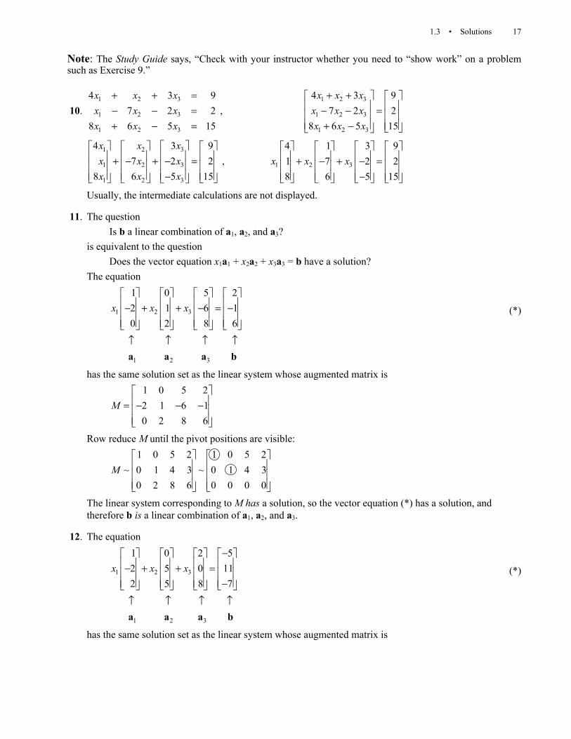
10. 1 2 3
1 2 3
1 2 3
4 3 97 2 2
8 6 5 15
x x xx x xx x x
+ + =− − =+ − =
, 1 2 3
1 2 3
1 2 3
4 3 97 2 2
8 6 5 15
x x xx x xx x x
+ + − − = + −
1 2 3
1 2 3
1 2 3
4 3 97 2 2
8 6 5 15
x x xx x xx x x
+ − + − = −
, 1 2 3
4 1 3 91 7 2 28 6 5 15
x x x + − + − = −
Usually, the intermediate calculations are not displayed.
11. The question Is b a linear combination of a1, a2, and a3? is equivalent to the question Does the vector equation x1a1 + x2a2 + x3a3 = b have a solution? The equation
1 2 3
1 2 3
1 0 5 22 1 6 10 2 8 6
x x x − + + − = −
↑ ↑ ↑ ↑a a a b
(*)
has the same solution set as the linear system whose augmented matrix is
1 0 5 22 1 6 10 2 8 6
M = − − −
Row reduce M until the pivot positions are visible:
1 0 5 2 1 0 5 2
~ 0 1 4 3 ~ 0 1 4 30 2 8 6 0 0 0 0
M
The linear system corresponding to M has a solution, so the vector equation (*) has a solution, and therefore b is a linear combination of a1, a2, and a3.
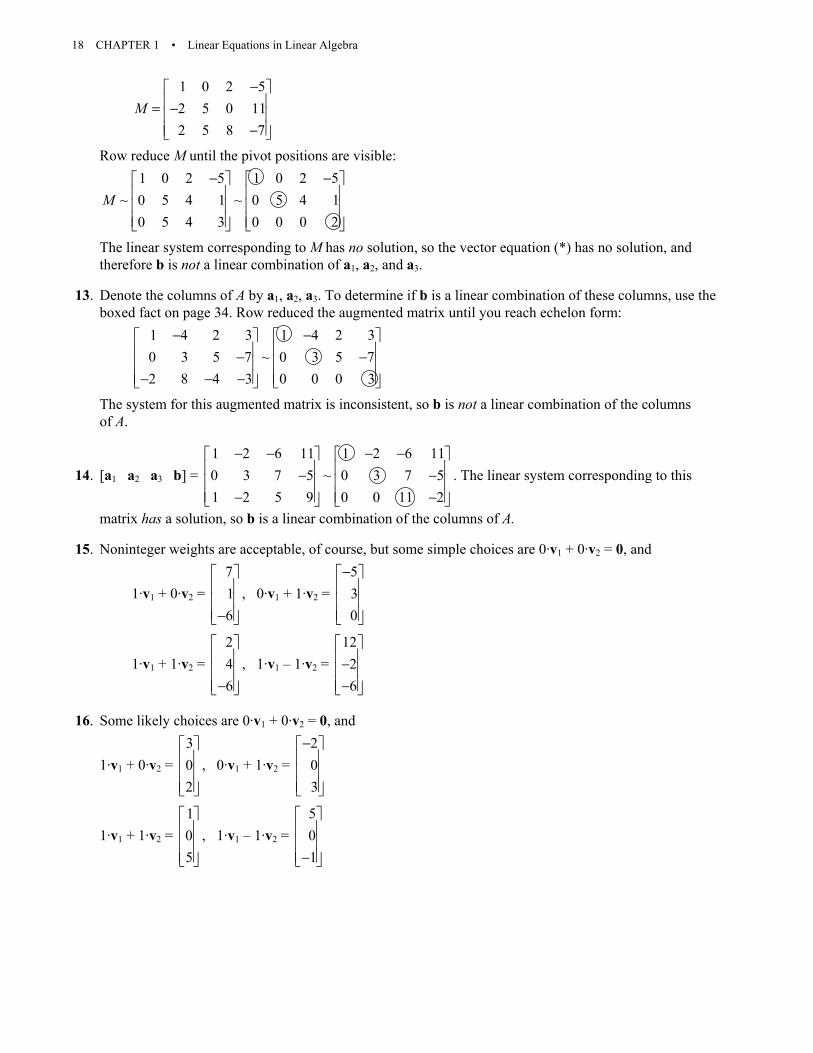
12. The equation
1 2 3
1 2 3
1 0 2 52 5 0 112 5 8 7
x x x−
− + + = −
↑ ↑ ↑ ↑a a a b
(*)
has the same solution set as the linear system whose augmented matrix is
18 CHAPTER 1 • Linear Equations in Linear Algebra
1 0 2 52 5 0 112 5 8 7
M−
= − −
Row reduce M until the pivot positions are visible:
1 0 2 5 1 0 2 5
~ 0 5 4 1 ~ 0 5 4 10 5 4 3 0 0 0 2
M− −
The linear system corresponding to M has no solution, so the vector equation (*) has no solution, and therefore b is not a linear combination of a1, a2, and a3.
13. Denote the columns of A by a1, a2, a3. To determine if b is a linear combination of these columns, use the boxed fact on page 34. Row reduced the augmented matrix until you reach echelon form:
1 4 2 3 1 4 2 30 3 5 7 ~ 0 3 5 72 8 4 3 0 0 0 3
− − − − − − −
The system for this augmented matrix is inconsistent, so b is not a linear combination of the columns of A.
14. [a1 a2 a3 b] = 1 2 6 11 1 2 6 110 3 7 5 ~ 0 3 7 51 2 5 9 0 0 11 2
− − − − − − − −
. The linear system corresponding to this
matrix has a solution, so b is a linear combination of the columns of A.
15. Noninteger weights are acceptable, of course, but some simple choices are 0·v1 + 0·v2 = 0, and
1·v1 + 0·v2 = 716
−
, 0·v1 + 1·v2 = 530
−
1·v1 + 1·v2 = 246
−
, 1·v1 – 1·v2 = 12
26
− −
16. Some likely choices are 0·v1 + 0·v2 = 0, and
1·v1 + 0·v2 = 302
, 0·v1 + 1·v2 = 203
−
1·v1 + 1·v2 = 105
, 1·v1 – 1·v2 = 501
−

1.3 • Solutions 19
17. [a1 a2 b] = 1 2 4 1 2 4 1 2 4 1 2 44 3 1 ~ 0 5 15 ~ 0 1 3 ~ 0 1 32 7 0 3 8 0 3 8 0 0 17h h h h
− − − − − − − − − + + +
. The vector b is
in Span{a1, a2} when h + 17 is zero, that is, when h = –17.
18. [v1 v2 y] = 1 3 1 3 1 30 1 5 ~ 0 1 5 ~ 0 1 52 8 3 0 2 3 2 0 0 7 2
h h h
h h
− − − − − − − − − + +
. The vector y is in
Span{v1, v2} when 7 + 2h is zero, that is, when h = –7/2.
19. By inspection, v2 = (3/2)v1. Any linear combination of v1 and v2 is actually just a multiple of v1. For instance,
av1 + bv2 = av1 + b(3/2)v2 = (a + 3b/2)v1 So Span{v1, v2} is the set of points on the line through v1 and 0.
Note: Exercises 19 and 20 prepare the way for ideas in Sections 1.4 and 1.7.
20. Span{v1, v2} is a plane in R3 through the origin, because the neither vector in this problem is a multiple of the other. Every vector in the set has 0 as its second entry and so lies in the xz-plane in ordinary 3-space. So Span{v1, v2} is the xz-plane.
21. Let y = hk
. Then [u v y] = 2 2 2 2
~1 1 0 2 / 2
h hk k h
− +
. This augmented matrix corresponds to
a consistent system for all h and k. So y is in Span{u, v} for all h and k.
22. Construct any 3×4 matrix in echelon form that corresponds to an inconsistent system. Perform sufficient row operations on the matrix to eliminate all zero entries in the first three columns.
23. a. False. The alternative notation for a (column) vector is (–4, 3), using parentheses and commas.
b. False. Plot the points to verify this. Or, see the statement preceding Example 3. If 52
−
were on
the line through 25
−
and the origin, then 52
−
would have to be a multiple of 25
−
, which is not
the case. c. True. See the line displayed just before Example 4. d. True. See the box that discusses the matrix in (5). e. False. The statement is often true, but Span{u, v} is not a plane when v is a multiple of u, or when
u is the zero vector.
24. a. True. See the beginning of the subsection Vectors in Rn. b. True. Use Fig. 7 to draw the parallelogram determined by u – v and v. c. False. See the first paragraph of the subsection Linear Combinations. d. True. See the statement that refers to Fig. 11. e. True. See the paragraph following the definition of Span{v1, …, vp}.
20 CHAPTER 1 • Linear Equations in Linear Algebra
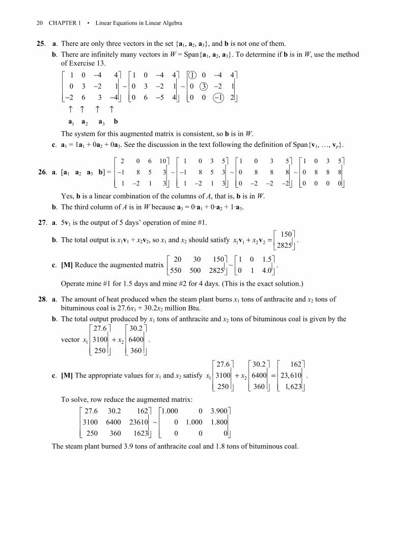
25. a. There are only three vectors in the set {a1, a2, a3}, and b is not one of them. b. There are infinitely many vectors in W = Span{a1, a2, a3}. To determine if b is in W, use the method
of Exercise 13.
1 2 3
1 0 4 4 1 0 4 4 1 0 4 40 3 2 1 ~ 0 3 2 1 ~ 0 3 2 12 6 3 4 0 6 5 4 0 0 1 2
− − − − − − − − − −
↑ ↑ ↑ ↑a a a b
The system for this augmented matrix is consistent, so b is in W. c. a1 = 1a1 + 0a2 + 0a3. See the discussion in the text following the definition of Span{v1, …, vp}.
26. a. [a1 a2 a3 b] = 2 0 6 10 1 0 3 5 1 0 3 5 1 0 3 5
1 8 5 3 ~ 1 8 5 3 ~ 0 8 8 8 ~ 0 8 8 8
1 2 1 3 1 2 1 3 0 2 2 2 0 0 0 0
− −
− − − − −
Yes, b is a linear combination of the columns of A, that is, b is in W. b. The third column of A is in W because a3 = 0·a1 + 0·a2 + 1·a3.
27. a. 5v1 is the output of 5 days’ operation of mine #1.
b. The total output is x1v1 + x2v2, so x1 and x2 should satisfy 1 1 2 2150
2825x x
+ =
v v .
c. [M] Reduce the augmented matrix 20 30 150 1 0 1.5
~550 500 2825 0 1 4.0
.
Operate mine #1 for 1.5 days and mine #2 for 4 days. (This is the exact solution.)
28. a. The amount of heat produced when the steam plant burns x1 tons of anthracite and x2 tons of bituminous coal is 27.6x1 + 30.2x2 million Btu.
b. The total output produced by x1 tons of anthracite and x2 tons of bituminous coal is given by the
vector 1 2
27.6 30.23100 6400250 360
x x +
.
c. [M] The appropriate values for x1 and x2 satisfy 1 2
27.6 30.2 1623100 6400 23,610250 360 1,623
x x + =
.
To solve, row reduce the augmented matrix:
27.6 30.2 162 1.000 0 3.900
3100 6400 23610 ~ 0 1.000 1.800250 360 1623 0 0 0
The steam plant burned 3.9 tons of anthracite coal and 1.8 tons of bituminous coal.

1.3 • Solutions 21
29. The total mass is 2 + 5 + 2 + 1 = 10. So v = (2v1 +5v2 + 2v3 + v4)/10. That is,
5 4 4 9 10 20 8 9 1.3
1 12 4 5 3 2 3 8 8 15 6 8 .910 10
3 2 1 6 6 10 2 6 0
− − + − − = − + + − + = − + − + = − − − − +
v
30. Let m be the total mass of the system. By definition,
11 1 1
1 ( ) kk k k
mmm mm m m
= + + = + +v v v v v
The second expression displays v as a linear combination of v1, …, vk, which shows that v is in Span{v1, …, vk}.
31. a. The center of mass is 0 8 2 10 / 31 1 1 11 1 4 23
⋅ + ⋅ + ⋅ =
.
b. The total mass of the new system is 9 grams. The three masses added, w1, w2, and w3, satisfy the equation
( ) ( ) ( )1 2 30 8 2 21 1 1 11 1 4 29
w w w
+ ⋅ + + ⋅ + + ⋅ =
which can be rearranged to
( ) ( ) ( )1 2 30 8 2 18
1 1 11 1 4 18
w w w
+ ⋅ + + ⋅ + + ⋅ =
and
1 2 30 8 2 81 1 4 12
w w w
⋅ + ⋅ + ⋅ =
The condition w1 + w2 + w3 = 6 and the vector equation above combine to produce a system of three equations whose augmented matrix is shown below, along with a sequence of row operations:
1 1 1 6 1 1 1 6 1 1 1 60 8 2 8 ~ 0 8 2 8 ~ 0 8 2 81 1 4 12 0 0 3 6 0 0 1 2
1 1 0 4 1 0 0 3.5 1 0 0 3.5
~ 0 8 0 4 ~ 0 8 0 4 ~ 0 1 0 .50 0 1 2 0 0 1 2 0 0 1 2
Answer: Add 3.5 g at (0, 1), add .5 g at (8, 1), and add 2 g at (2, 4).
Extra problem: Ignore the mass of the plate, and distribute 6 gm at the three vertices to make the center of mass at (2, 2). Answer: Place 3 g at (0, 1), 1 g at (8, 1), and 2 g at (2, 4).
32. See the parallelograms drawn on Fig. 15 from the text. Here c1, c2, c3, and c4 are suitable scalars. The darker parallelogram shows that b is a linear combination of v1 and v2, that is
c1v1 + c2v2 + 0·v3 = b

22 CHAPTER 1 • Linear Equations in Linear Algebra
The larger parallelogram shows that b is a linear combination of v1 and v3, that is, c4v1 + 0·v2 + c3v3 = b So the equation x1v1 + x2v2 + x3v3 = b has at least two solutions, not just one solution. (In fact, the
equation has infinitely many solutions.)
c2v2
c3v3
0
v3
c4v1
c1v1
v1
v2
b
33. a. For j = 1,…, n, the jth entry of (u + v) + w is (uj + vj) + wj. By associativity of addition in R, this entry equals uj + (vj + wj), which is the jth entry of u + (v + w). By definition of equality of vectors, (u + v) + w = u + (v + w).
b. For any scalar c, the jth entry of c(u + v) is c(uj + vj), and the jth entry of cu + cv is cuj + cvj (by definition of scalar multiplication and vector addition). These entries are equal, by a distributive law in R. So c(u + v) = cu + cv.
34. a. For j = 1,…, n, uj + (–1)uj = (–1)uj + uj = 0, by properties of R. By vector equality, u + (–1)u = (–1)u + u = 0. b. For scalars c and d, the jth entries of c(du) and (cd )u are c(duj) and (cd )uj, respectively. These
entries in R are equal, so the vectors c(du) and (cd)u are equal.
Note: When an exercise in this section involves a vector equation, the corresponding technology data (in the data files on the web) is usually presented as a set of (column) vectors. To use MATLAB or other technology, a student must first construct an augmented matrix from these vectors. The MATLAB note in the Study Guide describes how to do this. The appendices in the Study Guide give corresponding information about Maple, Mathematica, and the TI and HP calculators.
1.4 SOLUTIONS
Notes: Key exercises are 1–20, 27, 28, 31 and 32. Exercises 29, 30, 33, and 34 are harder. Exercise 34 anticipates the Invertible Matrix Theorem but is not used in the proof of that theorem.
1. The matrix-vector product Ax product is not defined because the number of columns (2) in the 3×2
matrix 4 21 60 1
−
does not match the number of entries (3) in the vector 327
−
.

1.4 • Solutions 23
2. The matrix-vector product Ax product is not defined because the number of columns (1) in the 3×1
matrix 261
−
does not match the number of entries (2) in the vector 51
−
.
3. 6 5 6 5 12 15 3
24 3 2 4 3 3 8 9 1
37 6 7 6 14 18 4
A− −
= − − = − − − = − + = − − −
x , and
6 5 6 2 5 ( 3) 3
24 3 ( 4) 2 ( 3) ( 3) 1
37 6 7 2 6 ( 3) 4
A⋅ + ⋅ − −
= − − = − ⋅ + − ⋅ − = − ⋅ + ⋅ − −
x
4. 1
8 3 4 8 3 4 8 3 4 71 1 1 1
5 1 2 5 1 2 5 1 2 81
A
− − + − = = ⋅ + ⋅ + ⋅ = = + +
x , and
1
8 3 4 8 1 3 1 ( 4) 1 71
5 1 2 5 1 1 1 2 1 81
A
− ⋅ + ⋅ + − ⋅ = = = ⋅ + ⋅ + ⋅
x
5. On the left side of the matrix equation, use the entries in the vector x as the weights in a linear combination of the columns of the matrix A:
5 1 8 4 8
5 1 3 22 7 3 5 16
− − ⋅ − ⋅ + ⋅ − ⋅ = − − −
6. On the left side of the matrix equation, use the entries in the vector x as the weights in a linear combination of the columns of the matrix A:
7 3 12 1 9
2 59 6 123 2 4
− − − ⋅ − ⋅ = − − −
7. The left side of the equation is a linear combination of three vectors. Write the matrix A whose columns are those three vectors, and create a variable vector x with three entries:
4 5 7 4 5 71 3 8 1 3 87 5 0 7 5 04 1 2 4 1 2
A
− − − − − − = = − − − −
and 1
2
3
xxx
=
x . Thus the equation Ax = b is
1
2
3
4 5 7 61 3 8 87 5 0 04 1 2 7
xxx
− − − − = − − −

24 CHAPTER 1 • Linear Equations in Linear Algebra
For your information: The unique solution of this equation is (5, 7, 3). Finding the solution by hand would be time-consuming.
Note: The skill of writing a vector equation as a matrix equation will be important for both theory and application throughout the text. See also Exercises 27 and 28.
8. The left side of the equation is a linear combination of four vectors. Write the matrix A whose columns are those four vectors, and create a variable vector with four entries:
4 4 5 3 4 4 5 32 5 4 0 2 5 4 0
A − − − −
= = − − , and
1
2
3
4
zzzz
=
z . Then the equation Az = b
is
1
2
3
4
4 4 5 3 42 5 4 0 13
zzzz
− − = −
.
For your information: One solution is (7, 3, 3, 1). The general solution is z1 = 6 + .75z3 – 1.25z4, z2 = 5 – .5z3 – .5z4, with z3 and z4 free.
9. The system has the same solution set as the vector equation
1 2 33 1 5 90 1 4 0
x x x−
+ + =
and this equation has the same solution set as the matrix equation
1
2
3
3 1 5 90 1 4 0
xxx
− =
10. The system has the same solution set as the vector equation
1 2
8 1 45 4 11 3 2
x x−
+ = −
and this equation has the same solution set as the matrix equation
1
2
8 1 45 4 11 3 2
xx
− = −
11. To solve Ax = b, row reduce the augmented matrix [a1 a2 a3 b] for the corresponding linear system:
1 2 4 2 1 2 4 2 1 2 4 2 1 2 0 6 1 0 0 00 1 5 2 ~ 0 1 5 2 ~ 0 1 5 2 ~ 0 1 0 3 ~ 0 1 0 32 4 3 9 0 0 5 5 0 0 1 1 0 0 1 1 0 0 1 1
− − − − − − − − −

1.4 • Solutions 25
The solution is 1
2
3
031
xxx
= = − =
. As a vector, the solution is x = 1
2
3
031
xxx
= −
.
12. To solve Ax = b, row reduce the augmented matrix [a1 a2 a3 b] for the corresponding linear system:
1 2 1 0 1 2 1 0 1 2 1 0 1 2 1 03 1 2 1 ~ 0 5 5 1 ~ 0 5 5 1 ~ 0 5 5 10 5 3 1 0 5 3 1 0 0 2 2 0 0 1 1
− − − − − −
1 2 0 1 1 2 0 1 1 0 0 3/ 5
~ 0 5 0 4 ~ 0 1 0 4 / 5 ~ 0 1 0 4 / 50 0 1 1 0 0 1 1 0 0 1 1
− − − − −
The solution is 1
2
3
3/ 54 /51
xxx
= = − =
. As a vector, the solution is x = 1
2
3
3/ 54 / 51
xxx
= −
.
13. The vector u is in the plane spanned by the columns of A if and only if u is a linear combination of the columns of A. This happens if and only if the equation Ax = u has a solution. (See the box preceding Example 3 in Section 1.4.) To study this equation, reduce the augmented matrix [A u]
3 5 0 1 1 4 1 1 4 1 1 42 6 4 ~ 2 6 4 ~ 0 8 12 ~ 0 8 121 1 4 3 5 0 0 8 12 0 0 0
− − − − − −
The equation Ax = u has a solution, so u is in the plane spanned by the columns of A. For your information: The unique solution of Ax = u is (5/2, 3/2).
14. Reduce the augmented matrix [A u] to echelon form:
5 8 7 2 1 3 0 2 1 3 0 2 1 3 0 20 1 1 3 ~ 0 1 1 3 ~ 0 1 1 3 ~ 0 1 1 31 3 0 2 5 8 7 2 0 7 7 8 0 0 0 29
− − − − − − − − − − −
The equation Ax = u has no solution, so u is not in the subset spanned by the columns of A.
15. The augmented matrix for Ax = b is 1
2
2 16 3
bb
− −
, which is row equivalent to 1
2 1
2 10 0 3
bb b
− +
.
This shows that the equation Ax = b is not consistent when 3b1 + b2 is nonzero. The set of b for which the equation is consistent is a line through the origin–the set of all points (b1, b2) satisfying b2 = –3b1.
16. Row reduce the augmented matrix [A b]: 1
2
3
1 3 43 2 6 , .5 1 8
bA b
b
− − = − = − −
b
1 1
2 2 1
3 3 1
1 3 4 1 3 43 2 6 ~ 0 7 6 35 1 8 0 14 12 5
b bb b bb b b
− − − − − − − + − − −

26 CHAPTER 1 • Linear Equations in Linear Algebra
1 1
2 1 2 1
3 1 2 1 1 2 3
1 3 4 1 3 4~ 0 7 6 3 0 7 6 3
0 0 0 5 2( 3 ) 0 0 0 2
b bb b b b
b b b b b b b
− − − − − − + = − − + − + + + +
The equation Ax = b is consistent if and only if b1 + 2b2 + b3 = 0. The set of such b is a plane through the origin in R3.
17. Row reduction shows that only three rows of A contain a pivot position:
1 3 0 3 1 3 0 3 1 3 0 3 1 3 0 31 1 1 1 0 2 1 4 0 2 1 4 0 2 1 4
~ ~ ~0 4 2 8 0 4 2 8 0 0 0 0 0 0 0 52 0 3 1 0 6 3 7 0 0 0 5 0 0 0 0
A
− − − − − − = − − − − − − −
Because not every row of A contains a pivot position, Theorem 4 in Section 1.4 shows that the equation Ax = b does not have a solution for each b in R4.
18. Row reduction shows that only three rows of B contain a pivot position:
1 3 2 2 1 3 2 2 1 3 2 2 1 3 2 20 1 1 5 0 1 1 5 0 1 1 5 0 1 1 5
~ ~ ~1 2 3 7 0 1 1 5 0 0 0 0 0 0 0 72 8 2 1 0 2 2 3 0 0 0 7 0 0 0 0
B
− − − − − − − − = − − − − − − − − − −
Because not every row of B contains a pivot position, Theorem 4 in Section 1.4 shows that the equation Bx = y does not have a solution for each y in R4.
19. The work in Exercise 17 shows that statement (d) in Theorem 4 is false. So all four statements in Theorem 4 are false. Thus, not all vectors in R4 can be written as a linear combination of the columns of A. Also, the columns of A do not span R4.
20. The work in Exercise 18 shows that statement (d) in Theorem 4 is false. So all four statements in Theorem 4 are false. Thus, not all vectors in R4 can be written as a linear combination of the columns of B. The columns of B certainly do not span R3, because each column of B is in R4, not R3. (This question was asked to alert students to a fairly common misconception among students who are just learning about spanning.)
21. Row reduce the matrix [v1 v2 v3] to determine whether it has a pivot in each row.
1 0 1 1 0 1 1 0 1 1 0 10 1 0 0 1 0 0 1 0 0 1 0
~ ~ ~ .1 0 0 0 0 1 0 0 1 0 0 10 1 1 0 1 1 0 0 1 0 0 0
− − − − − − −
The matrix [v1 v2 v3] does not have a pivot in each row, so the columns of the matrix do not span R4, by Theorem 4. That is, {v1, v2, v3} does not span R4.
Note: Some students may realize that row operations are not needed, and thereby discover the principle covered in Exercises 31 and 32.

1.4 • Solutions 27
22. Row reduce the matrix [v1 v2 v3] to determine whether it has a pivot in each row.
0 0 4 2 8 50 3 1 ~ 0 3 12 8 5 0 0 4
− − − − − − − −
The matrix [v1 v2 v3] has a pivot in each row, so the columns of the matrix span R4, by Theorem 4. That is, {v1, v2, v3} spans R4.
23. a. False. See the paragraph following equation (3). The text calls Ax = b a matrix equation. b. True. See the box before Example 3. c. False. See the warning following Theorem 4. d. True. See Example 4. e. True. See parts (c) and (a) in Theorem 4. f. True. In Theorem 4, statement (a) is false if and only if statement (d) is also false.
24. a. True. This statement is in Theorem 3. However, the statement is true without any "proof" because, by definition, Ax is simply a notation for x1a1 + ⋅ ⋅ ⋅ + xnan, where a1, …, an are the columns of A.
b. True. See Example 2. c. True, by Theorem 3. d. True. See the box before Example 2. Saying that b is not in the set spanned by the columns of A is the
same a saying that b is not a linear combination of the columns of A. e. False. See the warning that follows Theorem 4. f. True. In Theorem 4, statement (c) is false if and only if statement (a) is also false.
25. By definition, the matrix-vector product on the left is a linear combination of the columns of the matrix, in this case using weights –3, –1, and 2. So c1 = –3, c2 = –1, and c3 = 2.
26. The equation in x1 and x2 involves the vectors u, v, and w, and it may be viewed as
[ ] 1
2.
xx
=
u v w By definition of a matrix-vector product, x1u + x2v = w. The stated fact that
3u – 5v – w = 0 can be rewritten as 3u – 5v = w. So, a solution is x1 = 3, x2 = –5.
27. Place the vectors q1, q2, and q3 into the columns of a matrix, say, Q and place the weights x1, x2, and x3 into a vector, say, x. Then the vector equation becomes
Qx = v, where Q = [q1 q2 q3] and 1
2
3
xxx
=
x
Note: If your answer is the equation Ax = b, you need to specify what A and b are.
28. The matrix equation can be written as c1v1 + c2v2 + c3v3 + c4v4 + c5v5 = v6, where c1 = –3, c2 = 2, c3 = 4, c4 = –1, c5 = 2, and
1 2 3 4 5 63 5 4 9 7 8
, , , , ,5 8 1 2 4 1
− − = = = = = = − − −
v v v v v v

28 CHAPTER 1 • Linear Equations in Linear Algebra
29. Start with any 3×3 matrix B in echelon form that has three pivot positions. Perform a row operation (a row interchange or a row replacement) that creates a matrix A that is not in echelon form. Then A has the desired property. The justification is given by row reducing A to B, in order to display the pivot positions. Since A has a pivot position in every row, the columns of A span R3, by Theorem 4.
30. Start with any nonzero 3×3 matrix B in echelon form that has fewer than three pivot positions. Perform a row operation that creates a matrix A that is not in echelon form. Then A has the desired property. Since A does not have a pivot position in every row, the columns of A do not span R3, by Theorem 4.
31. A 3×2 matrix has three rows and two columns. With only two columns, A can have at most two pivot columns, and so A has at most two pivot positions, which is not enough to fill all three rows. By Theorem 4, the equation Ax = b cannot be consistent for all b in R3. Generally, if A is an m×n matrix with m > n, then A can have at most n pivot positions, which is not enough to fill all m rows. Thus, the equation Ax = b cannot be consistent for all b in R3.
32. A set of three vectors in cannot span R4. Reason: the matrix A whose columns are these three vectors has four rows. To have a pivot in each row, A would have to have at least four columns (one for each pivot), which is not the case. Since A does not have a pivot in every row, its columns do not span R4, by Theorem 4. In general, a set of n vectors in Rm cannot span Rm when n is less than m.
33. If the equation Ax = b has a unique solution, then the associated system of equations does not have any free variables. If every variable is a basic variable, then each column of A is a pivot column. So the
reduced echelon form of A must be
1 0 0
0 1 0
0 0 1
0 0 0
� �� �� �� �� �� �� �
.
Note: Exercises 33 and 34 are difficult in the context of this section because the focus in Section 1.4 is on existence of solutions, not uniqueness. However, these exercises serve to review ideas from Section 1.2, and they anticipate ideas that will come later.
34. If the equation Ax = b has a unique solution, then the associated system of equations does not have any free variables. If every variable is a basic variable, then each column of A is a pivot column. So the
reduced echelon form of A must be
1 0 0
0 1 0
0 0 1
� �� �� �� �� �
. Now it is clear that A has a pivot position in each row.
By Theorem 4, the columns of A span R3.
35. Given Ax1 = y1 and Ax2 = y2, you are asked to show that the equation Ax = w has a solution, where w = y1 + y2. Observe that w = Ax1 + Ax2 and use Theorem 5(a) with x1 and x2 in place of u and v, respectively. That is, w = Ax1 + Ax2 = A(x1 + x2). So the vector x = x1 + x2 is a solution of w = Ax.
36. Suppose that y and z satisfy Ay = z. Then 4z = 4Ay. By Theorem 5(b), 4Ay = A(4y). So 4z = A(4y), which shows that 4y is a solution of Ax = 4z. Thus, the equation Ax = 4z is consistent.
37. [M]
7 2 5 8 7 2 5 8 7 2 5 8
5 3 4 9 0 11/ 7 3/ 7 23/ 7 0 11/ 7 3/ 7 23/ 7~ ~
6 10 2 7 0 58/ 7 16 / 7 1/ 7 0 0 50 /11 189 /11
7 9 2 15 0 11 3 23 0 0 0 0
� � �� � � � � �� � � � � �� � � � � � �� � � � � �� � � � � �� �� � � � � �� �� � � � � �� � � � � �

1.4 • Solutions 29
or, approximately
7 2 5 80 1.57 .429 3.290 0 4.55 17.20 0 0 0
− − − −
, to three significant figures. The original matrix does not
have a pivot in every row, so its columns do not span R4, by Theorem 4.
38. [M]
5 7 4 9 5 7 4 9 5 7 4 96 8 7 5 0 2 / 5 11/ 5 29 / 5 0 2 / 5 11/ 5 29 / 5
~ ~4 4 9 9 0 8/ 5 29 / 5 81/ 5 0 0 3 79 11 16 7 0 8/ 5 44 / 5 116 / 5 0 0 * *
− − − − − − − − − − − − − − − − − − −
MATLAB shows starred entries for numbers that are essentially zero (to many decimal places). So, with pivots only in the first three rows, the original matrix has columns that do not span R4, by Theorem 4.
39. [M]
12 7 11 9 5 12 7 11 9 59 4 8 7 3 0 5/ 4 1/ 4 1/ 4 3/ 4
~6 11 7 3 9 0 15/ 2 3/ 2 3/ 2 13/ 24 6 10 5 12 0 11/ 3 19 / 3 2 31/ 3
− − − − − − − − − − − − − − − − − −
12 7 11 9 5 12 7 11 9 50 5/ 4 1/ 4 1/ 4 3/ 4 0 5/ 4 1/ 4 1/ 4 3/ 4
~ ~0 0 0 0 2 0 0 28/ 5 41/15 122 /150 0 28/ 5 41/15 122 /15 0 0 0 0 2
− − − − − − − − − −
The original matrix has a pivot in every row, so its columns span R4, by Theorem 4.
40. [M]
8 11 6 7 13 8 11 6 7 137 8 5 6 9 0 13/8 1/ 4 1/8 19 /8
~11 7 7 9 6 0 65/8 5/ 4 5/8 191/8
3 4 1 8 7 0 65/8 5/ 4 43/8 95/8
− − − − − − − − − − − − − − − −
8 11 6 7 13 8 11 6 7 130 13/8 1/ 4 1/8 19 /8 0 13/8 1/ 4 1/8 19 /8
~ ~0 0 0 0 12 0 0 0 6 00 0 0 6 0 0 0 0 0 12
− − − − − − − − − −
The original matrix has a pivot in every row, so its columns span R4, by Theorem 4.
41. [M] Examine the calculations in Exercise 39. Notice that the fourth column of the original matrix, say A, is not a pivot column. Let Ao be the matrix formed by deleting column 4 of A, let B be the echelon form obtained from A, and let Bo be the matrix obtained by deleting column 4 of B. The sequence of row operations that reduces A to B also reduces Ao to Bo. Since Bo is in echelon form, it shows that Ao has a pivot position in each row. Therefore, the columns of Ao span R4.
It is possible to delete column 3 of A instead of column 4. In this case, the fourth column of A becomes a pivot column of Ao, as you can see by looking at what happens when column 3 of B is deleted. For later work, it is desirable to delete a nonpivot column.

30 CHAPTER 1 • Linear Equations in Linear Algebra
Note: Exercises 41 and 42 help to prepare for later work on the column space of a matrix. (See Section 2.9 or 4.6.) The Study Guide points out that these exercises depend on the following idea, not explicitly mentioned in the text: when a row operation is performed on a matrix A, the calculations for each new entry depend only on the other entries in the same column. If a column of A is removed, forming a new matrix, the absence of this column has no affect on any row-operation calculations for entries in the other columns of A. (The absence of a column might affect the particular choice of row operations performed for some purpose, but that is not being considered here.)
42. [M] Examine the calculations in Exercise 40. The third column of the original matrix, say A, is not a pivot column. Let Ao be the matrix formed by deleting column 3 of A, let B be the echelon form obtained from A, and let Bo be the matrix obtained by deleting column 3 of B. The sequence of row operations that reduces A to B also reduces Ao to Bo. Since Bo is in echelon form, it shows that Ao has a pivot position in each row. Therefore, the columns of Ao span R4.
It is possible to delete column 2 of A instead of column 3. (See the remark for Exercise 41.) However, only one column can be deleted. If two or more columns were deleted from A, the resulting matrix would have fewer than four columns, so it would have fewer than four pivot positions. In such a case, not every row could contain a pivot position, and the columns of the matrix would not span R4, by Theorem 4.
Notes: At the end of Section 1.4, the Study Guide gives students a method for learning and mastering linear algebra concepts. Specific directions are given for constructing a review sheet that connects the basic definition of “span” with related ideas: equivalent descriptions, theorems, geometric interpretations, special cases, algorithms, and typical computations. I require my students to prepare such a sheet that reflects their choices of material connected with “span”, and I make comments on their sheets to help them refine their review. Later, the students use these sheets when studying for exams.
The MATLAB box for Section 1.4 introduces two useful commands gauss and bgauss that allow a student to speed up row reduction while still visualizing all the steps involved. The command B = gauss(A,1) causes MATLAB to find the left-most nonzero entry in row 1 of matrix A, and use that entry as a pivot to create zeros in the entries below, using row replacement operations. The result is a matrix that a student might write next to A as the first stage of row reduction, since there is no need to write a new matrix after each separate row replacement. I use the gauss command frequently in lectures to obtain an echelon form that provides data for solving various problems. For instance, if a matrix has 5 rows, and if row swaps are not needed, the following commands produce an echelon form of A:
B = gauss(A,1), B = gauss(B,2), B = gauss(B,3), B = gauss(B,4)
If an interchange is required, I can insert a command such as B = swap(B,2,5) . The command bgauss uses the left-most nonzero entry in a row to produce zeros above that entry. This command, together with scale, can change an echelon form into reduced echelon form.
The use of gauss and bgauss creates an environment in which students use their computer program the same way they work a problem by hand on an exam. Unless you are able to conduct your exams in a computer laboratory, it may be unwise to give students too early the power to obtain reduced echelon forms with one command—they may have difficulty performing row reduction by hand during an exam. Instructors whose students use a graphic calculator in class each day do not face this problem. In such a case, you may wish to introduce rref earlier in the course than Chapter 4 (or Section 2.8), which is where I finally allow students to use that command.
1.5 SOLUTIONS
Notes: The geometry helps students understand Span{u, v}, in preparation for later discussions of subspaces. The parametric vector form of a solution set will be used throughout the text. Figure 6 will appear again in Sections 2.9 and 4.8.

1.5 • Solutions 31
For solving homogeneous systems, the text recommends working with the augmented matrix, although no calculations take place in the augmented column. See the Study Guide comments on Exercise 7 that illustrate two common student errors.
All students need the practice of Exercises 1–14. (Assign all odd, all even, or a mixture. If you do not assign Exercise 7, be sure to assign both 8 and 10.) Otherwise, a few students may be unable later to find a basis for a null space or an eigenspace. Exercises 29–34 are important. Exercises 33 and 34 help students later understand how solutions of Ax = 0 encode linear dependence relations among the columns of A. Exercises 35–38 are more challenging. Exercise 37 will help students avoid the standard mistake of forgetting that Theorem 6 applies only to a consistent equation Ax = b.
1. Reduce the augmented matrix to echelon form and circle the pivot positions. If a column of the coefficient matrix is not a pivot column, the corresponding variable is free and the system of equations has a nontrivial solution. Otherwise, the system has only the trivial solution.
2 5 8 0 2 5 8 0 2 5 8 02 7 1 0 ~ 0 12 9 0 ~ 0 12 9 04 2 7 0 0 12 9 0 0 0 0 0
− − − − − − − −
The variable x3 is free, so the system has a nontrivial solution.
2. 1 3 7 0 1 3 7 0 1 3 7 02 1 4 0 ~ 0 5 10 0 ~ 0 5 10 01 2 9 0 0 5 2 0 0 0 12 0
− − − − − − −
There is no free variable; the system has only the trivial solution.
3. 3 5 7 0 3 5 7 0
~6 7 1 0 0 3 15 0
− − − − − −
. The variable x3 is free; the system has nontrivial solutions.
An alert student will realize that row operations are unnecessary. With only two equations, there can be at most two basic variables. One variable must be free. Refer to Exercise 31 in Section 1.2.
4. 5 7 9 0 1 2 6 0 1 2 6 0
~ ~1 2 6 0 5 7 9 0 0 3 39 0
− − − − − −
. x3 is a free variable; the system has
nontrivial solutions. As in Exercise 3, row operations are unnecessary.
5. 1 3 1 0 1 3 1 0 1 0 5 0 1 0 5 04 9 2 0 ~ 0 3 6 0 ~ 0 3 6 0 ~ 0 1 2 00 3 6 0 0 3 6 0 0 0 0 0 0 0 0 0
− − − − − − − −
1 3
2 3
5 02 0
0 0
x xx x
− =+ =
=. The variable x3 is free, x1 = 5x3, and x2 = –2x3.
In parametric vector form, the general solution is 1 3
2 3 3
3 3
5 52 2
1
x xx x xx x
= = − = −
x .

32 CHAPTER 1 • Linear Equations in Linear Algebra
6. 1 3 5 0 1 3 5 0 1 3 5 0 1 0 4 01 4 8 0 ~ 0 1 3 0 ~ 0 1 3 0 ~ 0 1 3 03 7 9 0 0 2 6 0 0 0 0 0 0 0 0 0
− − − − − − − − − −
1 3
2 3
4 03 0
0 0
x xx x
+ =− =
=. The variable x3 is free, x1 = –4x3, and x2 = 3x3.
In parametric vector form, the general solution is 1 3
2 3 3
3 3
4 43 3
1
x xx x xx x
− − = = =
x .
7. 1 3 3 7 0 1 0 9 8 0
~0 1 4 5 0 0 1 4 5 0
− − − −
. 1 3 4
2 3 4
9 8 04 5 0
x x xx x x
+ − =− + =
The basic variables are x1 and x2, with x3 and x4 free. Next, x1 = –9x3 + 8x4, and x2 = 4x3 – 5x4. The general solution is
1 3 4 43
2 3 4 433 4
3 3 3
4 4 4
9 8 89 9 84 5 54 4 5
0 1 00 0 1
x x x xxx x x xx
x xx x xx x x
− + − − − − − = = = + = +
x
8. 1 2 9 5 0 1 0 5 7 0
~0 1 2 6 0 0 1 2 6 0
− − − − − −
. 1 3 4
2 3 4
5 7 02 6 0
x x xx x x
− − =+ − =
The basic variables are x1 and x2, with x3 and x4 free. Next, x1 = 5x3 + 7x4 and x2 = –2x3 + 6x4. The general solution in parametric vector form is
1 3 4 43
2 3 4 433 4
3 3 3
4 4 4
5 7 75 5 72 6 62 2 6
0 1 00 0 1
x x x xxx x x xx
x xx x xx x x
+ − + − − = = = + = +
x
9. 3 9 6 0 1 3 2 0 1 3 2 0
~ ~1 3 2 0 3 9 6 0 0 0 0 0
− − − − − −
1 2 33 2 00 0
x x x− + ==
.
The solution is x1 = 3x2 – 2x3, with x2 and x3 free. In parametric vector form,
2 3 2 3
2 2 2 3
3 3
3 2 3 2 3 20 1 0
0 0 1
x x x xx x x xx x
− − − = = + = +
x .
10. 1 3 0 4 0 1 3 0 4 0
~2 6 0 8 0 0 0 0 0 0
− − −
1 2 43 4 00 0
x x x− − ==
.
The only basic variable is x1, so x2, x3, and x4 are free. (Note that x3 is not zero.) Also, x1 = 3x2 + 4x4. The general solution is

1.5 • Solutions 33
1 2 4 42
2 2 22 3 4
3 3 3
4 4 4
3 4 43 0 3 0 400 1 0 000 0 1 0
0 0 0 0 1
x x x xxx x x
x x xx x xx x x
+ = = = + + = + +
x
11.
1 4 2 0 3 5 0 1 4 2 0 0 7 0 1 4 0 0 0 5 00 0 1 0 0 1 0 0 0 1 0 0 1 0 0 0 1 0 0 1 0
~ ~0 0 0 0 1 4 0 0 0 0 0 1 4 0 0 0 0 0 1 4 00 0 0 0 0 0 0 0 0 0 0 0 0 0 0 0 0 0 0 0 0
− − − − − − − − − − − −
1 2 6
3 6
5 6
4 5 00
4 00 0
x x xx x
x x
− + =− =− =
=
. The basic variables are x1, x3, and x5. The remaining variables are free.
In particular, x4 is free (and not zero as some may assume). The solution is x1 = 4x2 – 5x6, x3 = x6, x5 = 4x6, with x2, x4, and x6 free. In parametric vector form,
1 2 6 62
2 2 2
3 6 62 4
4 4 4
5 6 6
6 6 6
4 5 54 0 4 000 1 0
0 0 0 000 0
4 40 0 00 0 0
x x x xxx x xx x x
x xx x xx x xx x x
− −
= = = + + = +
x 6
501
1 00 40 1
x
−
+
↑ ↑ ↑u v w
Note: The Study Guide discusses two mistakes that students often make on this type of problem.
12.
1 5 2 6 9 0 0 1 5 2 6 9 0 0 1 5 0 8 1 0 00 0 1 7 4 8 0 0 0 1 7 4 0 0 0 0 1 7 4 0 0
~ ~0 0 0 0 0 1 0 0 0 0 0 0 1 0 0 0 0 0 0 1 00 0 0 0 0 0 0 0 0 0 0 0 0 0 0 0 0 0 0 0 0
− − − − − −
1 2 4 5
3 4 5
6
5 8 07 4 0
00 0
x x x xx x x
x
+ + + =− + =
==
.
The basic variables are x1, x3, and x6; the free variables are x2, x4, and x5. The general solution is x1 = –5x2 – 8x4 – x5, x3 = 7x4 – 4x5, and x6 = 0. In parametric vector form, the solution is

34 CHAPTER 1 • Linear Equations in Linear Algebra
1 2 4 5 2 4 5
2 2 2
3 4 5 4 52
4 4 4
5 5 5
6
5 8 5 8 50 0 1
7 4 0 7 4 00 0 00 0 0
0 0 0 0 0
x x x x x x xx x xx x x x x
xx x xx x xx
− − − − − − − − −
= = = + + =
x 4 5
8 10 07 41 00 10 0
x x
− −
−
+ +
13. To write the general solution in parametric vector form, pull out the constant terms that do not involve the free variable:
1 3 3
2 3 3 3 3
3 3 3
5 4 5 4 5 42 7 2 7 2 7 .
0 0 1
x x xx x x x xx x x
+ = = − − = − + − = − + − = +
↑ ↑
x p q
p q
Geometrically, the solution set is the line through 520
−
in the direction of 471
−
.
14. To write the general solution in parametric vector form, pull out the constant terms that do not involve the free variable:
1 4 4
2 4 44 4
3 4 4
4 4 4
3 30 0 38 8 8 12 5 52 2 5
0 0 1
x x xx x x
x xx x xx x x
+ = = = + = + = + − − −
↑ ↑
x p q
p q
The solution set is the line through p in the direction of q.
15. Row reduce the augmented matrix for the system:
1 3 1 1 1 3 1 1 1 3 1 14 9 2 1 ~ 0 3 6 3 ~ 0 3 6 30 3 6 3 0 3 6 3 0 0 0 0
− − − − − − − − −
1 3 1 1 1 0 5 2
~ 0 1 2 1 ~ 0 1 2 10 0 0 0 0 0 0 0
− −
. 1 3
2 3
5 22 10 0
x xx x
− = −+ =
=.
Thus x1 = –2 + 5x3, x2 = 1 – 2x3, and x3 is free. In parametric vector form,
1 3 3
2 3 3 3
3 3 3
2 5 2 5 2 51 2 1 2 1 2
0 0 1
x x xx x x xx x x
− + − − = = − = + − = + −
x

1.5 • Solutions 35
The solution set is the line through 210
−
, parallel to the line that is the solution set of the homogeneous
system in Exercise 5.
16. Row reduce the augmented matrix for the system:
1 3 5 4 1 3 5 4 1 3 5 4 1 0 4 51 4 8 7 ~ 0 1 3 3 ~ 0 1 3 3 ~ 0 1 3 33 7 9 6 0 2 6 6 0 0 0 0 0 0 0 0
− − − − − − − − − − − −
1 3
2 3
4 53 30 0
x xx x
+ = −− =
=. Thus x1 = –5 – 4x3, x2 = 3 + 3x3, and x3 is free. In parametric vector form,
1 3 3
2 3 3 3
3 3 3
5 4 5 4 5 43 3 3 3 3 3
0 0 1
x x xx x x xx x x
− − − − − − = = + = + = +
x
The solution set is the line through 530
−
, parallel to the line that is the solution set of the homogeneous
system in Exercise 6.
17. Solve x1 + 9x2 – 4x3 = –2 for the basic variable: x1 = –2 – 9x2 + 4x3, with x2 and x3 free. In vector form, the solution is
1 2 3 2 3
2 2 2 2 3
3 3 3
2 9 4 2 9 4 2 9 40 0 0 1 00 0 0 0 1
x x x x xx x x x xx x x
− − + − − − − = = = + + = + +
x
The solution of x1 + 9x2 – 4x3 = 0 is x1 = –9x2 + 4x3, with x2 and x3 free. In vector form,
1 2 3 2 3
2 2 2 2 3
3 3 3
9 4 9 4 9 40 1 0
0 0 1
x x x x xx x x x xx x x
− + − − = = = + = +
x = x2u + x3v
The solution set of the homogeneous equation is the plane through the origin in R3 spanned by u and v. The solution set of the nonhomogeneous equation is parallel to this plane and passes through the
point p = 200
−
.
18. Solve x1 – 3x2 + 5x3 = 4 for the basic variable: x1 = 4 + 3x2 – 5x3, with x2 and x3 free. In vector form, the solution is
1 2 3 2 3
2 2 2 2 3
3 3 3
4 3 5 4 3 5 4 3 50 0 0 1 00 0 0 0 1
x x x x xx x x x xx x x
+ − − − = = = + + = + +
x

36 CHAPTER 1 • Linear Equations in Linear Algebra
The solution of x1 – 3x2 + 5x3 = 0 is x1 = 3x2 – 5x3, with x2 and x3 free. In vector form,
1 2 3 2 3
2 2 2 2 3
3 3 3
3 5 3 5 3 50 1 0
0 0 1
x x x x xx x x x xx x x
− − − = = = + = +
x = x2u + x3v
The solution set of the homogeneous equation is the plane through the origin in R3 spanned by u and v. The solution set of the nonhomogeneous equation is parallel to this plane and passes through the
point p = 400
.
19. The line through a parallel to b can be written as x = a + t b, where t represents a parameter:
x = 1
2
2 50 3
xt
x− −
= +
, or 1
2
2 53
x tx t
= − − =
20. The line through a parallel to b can be written as x = a + tb, where t represents a parameter:
x = 1
2
3 74 8
xt
x−
= + − , or 1
2
3 74 8
x tx t
= − = − +
21. The line through p and q is parallel to q – p. So, given 2 3
and5 1
− = = −
p q , form
3 2 51 ( 5) 6− − −
− = = − − q p , and write the line as x = p + t(q – p) =
2 55 6
t−
+ − .
22. The line through p and q is parallel to q – p. So, given 6 0
and 3 4
− = = −
p q , form
0 ( 6) 64 3 7
− − − = = − − −
q p , and write the line as x = p + t(q – p) = 6 63 7
t−
+ −
Note: Exercises 21 and 22 prepare for Exercise 27 in Section 1.8.
23. a. True. See the first paragraph of the subsection titled Homogeneous Linear Systems. b. False. The equation Ax = 0 gives an implicit description of its solution set. See the subsection entitled
Parametric Vector Form. c. False. The equation Ax = 0 always has the trivial solution. The box before Example 1 uses the word
nontrivial instead of trivial. d. False. The line goes through p parallel to v. See the paragraph that precedes Fig. 5. e. False. The solution set could be empty! The statement (from Theorem 6) is true only when there
exists a vector p such that Ap = b.
24. a. False. A nontrivial solution of Ax = 0 is any nonzero x that satisfies the equation. See the sentence before Example 2. b. True. See Example 2 and the paragraph following it.

1.5 • Solutions 37
c. True. If the zero vector is a solution, then b = Ax = A0 = 0. d. True. See the paragraph following Example 3. e. False. The statement is true only when the solution set of Ax = 0 is nonempty. Theorem 6 applies
only to a consistent system.
25. Suppose p satisfies Ax = b. Then Ap = b. Theorem 6 says that the solution set of Ax = b equals the set S ={w : w = p + vh for some vh such that Avh = 0}. There are two things to prove: (a) every vector in S satisfies Ax = b, (b) every vector that satisfies Ax = b is in S. a. Let w have the form w = p + vh, where Avh = 0. Then Aw = A(p + vh) = Ap + Avh. By Theorem 5(a) in section 1.4 = b + 0 = b So every vector of the form p + vh satisfies Ax = b. b. Now let w be any solution of Ax = b, and set vh = w − p. Then Avh = A(w – p) = Aw – Ap = b – b = 0 So vh satisfies Ax = 0. Thus every solution of Ax = b has the form w = p + vh.
26. (Geometric argument using Theorem 6.) Since Ax = b is consistent, its solution set is obtained by translating the solution set of Ax = 0, by Theorem 6. So the solution set of Ax = b is a single vector if and only if the solution set of Ax = 0 is a single vector, and that happens if and only if Ax = 0 has only the trivial solution.
(Proof using free variables.) If Ax = b has a solution, then the solution is unique if and only if there are no free variables in the corresponding system of equations, that is, if and only if every column of A is a pivot column. This happens if and only if the equation Ax = 0 has only the trivial solution.
27. When A is the 3×3 zero matrix, every x in R3 satisfies Ax = 0. So the solution set is all vectors in R3.
28. No. If the solution set of Ax = b contained the origin, then 0 would satisfy A0= b, which is not true since b is not the zero vector.
29. a. When A is a 3×3 matrix with three pivot positions, the equation Ax = 0 has no free variables and hence has no nontrivial solution.
b. With three pivot positions, A has a pivot position in each of its three rows. By Theorem 4 in Section 1.4, the equation Ax = b has a solution for every possible b. The term "possible" in the exercise means that the only vectors considered in this case are those in R3, because A has three rows.
30. a. When A is a 3×3 matrix with two pivot positions, the equation Ax = 0 has two basic variables and one free variable. So Ax = 0 has a nontrivial solution.
b. With only two pivot positions, A cannot have a pivot in every row, so by Theorem 4 in Section 1.4, the equation Ax = b cannot have a solution for every possible b (in R3).
31. a. When A is a 3×2 matrix with two pivot positions, each column is a pivot column. So the equation Ax = 0 has no free variables and hence no nontrivial solution. b. With two pivot positions and three rows, A cannot have a pivot in every row. So the equation Ax = b
cannot have a solution for every possible b (in R3), by Theorem 4 in Section 1.4.
32. a. When A is a 2×4 matrix with two pivot positions, the equation Ax = 0 has two basic variables and two free variables. So Ax = 0 has a nontrivial solution. b. With two pivot positions and only two rows, A has a pivot position in every row. By Theorem 4 in
Section 1.4, the equation Ax = b has a solution for every possible b (in R2).

38 CHAPTER 1 • Linear Equations in Linear Algebra
33. Look at 1 2
2 67 213 9
x x− − + − −
and notice that the second column is 3 times the first. So suitable values for
x1 and x2 would be 3 and –1 respectively. (Another pair would be 6 and –2, etc.) Thus 31
= −
x
satisfies Ax = 0.
34. Inspect how the columns a1 and a2 of A are related. The second column is –3/2 times the first. Put
another way, 3a1 + 2a2 = 0. Thus 32
satisfies Ax = 0.
Note: Exercises 33 and 34 set the stage for the concept of linear dependence.
35. Look for A = [a1 a2 a3] such that 1·a1 + 1a2 + 1·a3 = 0. That is, construct A so that each row sum (the sum of the entries in a row) is zero.
36. Look for A = [a1 a2 a3] such that 1·a1 – 2·a2 + 1·a3 = 0. That is, construct A so that the sum of the first and third columns is twice the second column.
37. Since the solution set of Ax = 0 contains the point (4,1), the vector x = (4,1) satisfies Ax = 0. Write this equation as a vector equation, using a1 and a2 for the columns of A:
4·a1 + 1·a2 = 0 Then a2 = –4a1. So choose any nonzero vector for the first column of A and multiply that column by – 4
to get the second column of A. For example, set 1 41 4
A−
= − .
Finally, the only way the solution set of Ax = b could not be parallel to the line through (1,4) and the origin is for the solution set of Ax = b to be empty. This does not contradict Theorem 6, because that theorem applies only to the case when the equation Ax = b has a nonempty solution set. For b, take any vector that is not a multiple of the columns of A.
Note: In the Study Guide, a “Checkpoint” for Section 1.5 will help students with Exercise 37.
38. No. If Ax = y has no solution, then A cannot have a pivot in each row. Since A is 3×3, it has at most two pivot positions. So the equation Ax = z for any z has at most two basic variables and at least one free variable. Thus, the solution set for Ax = z is either empty or has infinitely many elements.
39. If u satisfies Ax = 0, then Au = 0. For any scalar c, Theorem 5(b) in Section 1.4 shows that A(cu) = cAu = c·0 = 0.
40. Suppose Au = 0 and Av = 0. Then, since A(u + v) = Au + Av by Theorem 5(a) in Section 1.4, A(u + v) = Au + Av = 0 + 0 = 0. Now, let c and d be scalars. Using both parts of Theorem 5, A(cu + dv) = A(cu) + A(dv) = cAu + dAv = c0 + d0 = 0.
Note: The MATLAB box in the Study Guide introduces the zeros command, in order to augment a matrix with a column of zeros.

1.6 • Solutions 39
1.6 SOLUTIONS
1. Fill in the exchange table one column at a time. The entries in a column describe where a sector's output goes. The decimal fractions in each column sum to 1.
Distribution of Output From:
Goods Services Purchased by:output input
.2 .7 Goods
.8 .3 Services
↓ ↓→→
Denote the total annual output (in dollars) of the sectors by pG and pS. From the first row, the total input to the Goods sector is .2 pG + .7 pS. The Goods sector must pay for that. So the equilibrium prices must satisfy
G G S
income expenses= .2 .7p p p+
From the second row, the input (that is, the expense) of the Services sector is .8 pG + .3 pS. The equilibrium equation for the Services sector is
S G S
income expenses= .8 .3p p p+
Move all variables to the left side and combine like terms:
G S
G S
.8 .7 0
.8 .7 0p pp p
− =− + =
Row reduce the augmented matrix: .8 .7 0 .8 .7 0 1 .875 0
~ ~.8 .7 0 0 0 0 0 0 0
− − − −
The general solution is pG = .875 pS, with pS free. One equilibrium solution is pS = 1000 and pG = 875. If one uses fractions instead of decimals in the calculations, the general solution would be written pG = (7/8) pS, and a natural choice of prices might be pS = 80 and pG = 70. Only the ratio of the prices is important: pG = .875 pS. The economic equilibrium is unaffected by a proportional change in prices.
2. Take some other value for pS, say 200 million dollars. The other equilibrium prices are then pC = 188 million, pE = 170 million. Any constant nonnegative multiple of these prices is a set of equilibrium prices, because the solution set of the system of equations consists of all multiples of one vector. Changing the unit of measurement to, say, European euros has the same effect as multiplying all equilibrium prices by a constant. The ratios of the prices remain the same, no matter what currency is used.
3. a. Fill in the exchange table one column at a time. The entries in a column describe where a sector’s output goes. The decimal fractions in each column sum to 1.

40 CHAPTER 1 • Linear Equations in Linear Algebra
Distribution of Output From: PurchasedChemicals Fuels Machinery by:
output input.2 .8 .4 Chemicals.3 .1 .4 Fuels.5 .1 .2 Machinery
↓ ↓ ↓
b. Denote the total annual output (in dollars) of the sectors by pC, pF, and pM. From the first row of the table, the total input to the Chemical & Metals sector is .2 pC + .8 pF + .4 pM. So the equillibrium prices must satisfy
C C F M
income expenses= .2 .8 .4p p p p+ +
From the second and third rows of the table, the income/expense requirements for the Fuels & Power sector and the Machinery sector are, respectively,
F C F M
M C F M
.3 .1 .4.5 .1 .2
p p p pp p p p
= + += + +
Move all variables to the left side and combine like terms:
C F M
C F M
C F M
.8 – .8 – .4 0–.3 .9 – .4 0–.5 – .1 .8 0
p p pp p pp p p
=+ =
+ =
c. [M] You can obtain the reduced echelon form with a matrix program. Actually, hand calculations are not too messy. To simplify the calculations, first scale each row of the augmented matrix by 10, then continue as usual.
8 8 4 0 1 1 .5 0 1 1 .5 03 9 4 0 ~ 3 9 4 0 ~ 0 6 5.5 05 1 8 0 5 1 8 0 0 6 5.5 0
1 1 .5 0 1 0 1.417 0 The number of decimal~ 0 1 .917 0 ~ 0 1 .917 0 places displayed is
0 0 0 0 0 0 0 0 somewhat arbit
− − − − − − − − − − − − − − − −
− − − − − rary.
The general solution is pC = 1.417 pM, pF = .917 pM, with pM free. If pM is assigned the value 100, then pC = 141.7 and pF = 91.7. Note that only the ratios of the prices are determined. This makes sense, for if the were converted from, say, dollars to yen or Euros, the inputs and outputs of each sector would still balance. The economic equilibrium is not affected by a proportional change in prices.

1.6 • Solutions 41
4. a. Fill in the exchange table one column at a time. The entries in each column must sum to 1.
Distribution of Output From :
Purchased by :Agric. Energy Manuf . Transp.output input
.65 .30 .30 .20 Agric.
.10 .10 .15 .10 Energy
.25 .35 .15 .30 Manuf .0 .25 .40 .40 Transp.
↓ ↓ ↓ ↓→→→→
b. Denote the total annual output of the sectors by pA, pE, pM, and pT, respectively. From the first row of the table, the total input to Agriculture is .65pA + .30pE + .30pM + .20 pT. So the equilibrium prices must satisfy
A A E M T
income expenses.65 .30 .30 .20p p p p p= + + +
From the second, third, and fourth rows of the table, the equilibrium equations are
E A E M T
M A E M T
T E M T
.10 .10 .15 .10
.25 .35 .15 .30.25 .40 .40
p p p p pp p p p pp p p p
= + + += + + += + +
Move all variables to the left side and combine like terms:
A E M T
A E M T
A E M T
E M T
.35 .30 .30 .20 0
.10 .90 .15 .10 0
.25 .35 .85 .30 0.25 .40 .60 0
p p p pp p p pp p p p
p p p
− − − =− + − − =− − + − =
− − + =
Use gauss, bgauss, and scale operations to reduce the augmented matrix to reduced echelon form
.35 .3 .3 .2 0 .35 .3 0 .55 0 .35 0 0 .71 00 .81 .24 .16 0 0 .81 0 .43 0 0 1 0 .53 0
~ ~0 0 1.0 1.17 0 0 0 1 1.17 0 0 0 1 1.17 00 0 0 0 0 0 0 0 0 0 0 0 0 0 0
− − − − − − − − − − − − −
Scale the first row and solve for the basic variables in terms of the free variable pT, and obtain pA = 2.03pT, pE = .53pT, and pM = 1.17pT. The data probably justifies at most two significant figures, so take pT = 100 and round off the other prices to pA = 200, pE = 53, and pM = 120.
5. The following vectors list the numbers of atoms of boron (B), sulfur (S), hydrogen (H), and oxygen (O):
2 3 2 3 3 2
2 0 1 0 boron3 0 0 1 sulfur
B S : , H O: , H BO : , H S:0 2 3 2 hydrogen0 1 3 0 oxygen
The coefficients in the equation x1⋅B2S3 + x2⋅H20 → x3⋅H3BO3 + x4⋅H2S satisfy

42 CHAPTER 1 • Linear Equations in Linear Algebra
1 2 3 4
2 0 1 03 0 0 10 2 3 20 1 3 0
x x x x
+ = +
Move the right terms to the left side (changing the sign of each entry in the third and fourth vectors) and row reduce the augmented matrix of the homogeneous system:
2 0 1 0 0 2 0 1 0 0 2 0 1 0 0 2 0 1 0 03 0 0 1 0 0 0 3/ 2 1 0 0 1 3 0 0 0 1 3 0 0
~ ~ ~0 2 3 2 0 0 2 3 2 0 0 0 3/ 2 1 0 0 0 3/ 2 1 00 1 3 0 0 0 1 3 0 0 0 2 3 2 0 0 0 3 2 0
− − − − − − − − − − − − − − − − − − −
2 0 1 0 0 2 0 0 2 / 3 0 1 0 0 1/ 3 00 1 3 0 0 0 1 0 2 0 0 1 0 2 0
~ ~ ~0 0 1 2 / 3 0 0 0 1 2 / 3 0 0 0 1 2 / 3 00 0 3 2 0 0 0 0 0 0 0 0 0 0 0
− − − − − − − − − −
The general solution is x1 = (1/3) x4, x2 = 2x4, x3 = (2/3) x4, with x4 free. Take x4 = 3. Then x1 = 1, x2 = 6, and x3 = 2. The balanced equation is
B2S3 + 6H20 → 2H3BO3 + 3H2S
6. The following vectors list the numbers of atoms of sodium (Na), phosphorus (P), oxygen (O), barium (Ba), and nitrogen(N):
3 4 3 2 3 4 2 3
3 0 0 1 sodium1 0 2 0 phosphorus
Na PO : , Ba(NO ) : , Ba (PO ) : , NaNO :4 6 8 3 oxygen0 1 3 0 barium0 2 0 1 nitrogen
The coefficients in the equation x1⋅Na3PO4 + x2⋅Ba(NO3)2 → x3⋅Ba3(PO4)2 + x4⋅NaNO3 satisfy
1 2 3 4
3 0 0 11 0 2 04 6 8 30 1 3 00 2 0 1
x x x x
+ = +
Move the right terms to the left side (changing the sign of each entry in the third and fourth vectors) and row reduce the augmented matrix of the homogeneous system:
3 0 0 1 0 1 0 2 0 0 1 0 2 0 0 1 0 2 0 01 0 2 0 0 3 0 0 1 0 0 0 6 1 0 0 1 3 0 0
~ ~ ~4 6 8 3 0 4 6 8 3 0 0 6 0 3 0 0 6 0 3 00 1 3 0 0 0 1 3 0 0 0 1 3 0 0 0 0 6 1 00 2 0 1 0 0 2 0 1 0 0 2 0 1 0 0 2 0 1 0
− − − − − − − − − − − − − − − − − − − − − −

1.6 • Solutions 43
1 0 2 0 0 1 0 2 0 0 1 0 0 1/ 3 00 1 3 0 0 0 1 3 0 0 0 1 0 1/ 2 0
~ ~ ~0 0 18 3 0 0 0 1 1/ 6 0 0 0 1 1/ 6 00 0 6 1 0 0 0 0 0 0 0 0 0 0 00 0 6 1 0 0 0 0 0 0 0 0 0 0 0
− − − − − − − − − − −
The general solution is x1 = (1/3)x4, x2 = (1/2)x4, x3 = (1/6)x4, with x4 free. Take x4 = 6. Then x1 = 2, x2 = 3, and x3 = 1. The balanced equation is
2Na3PO4 + 3Ba(NO3)2 → Ba3(PO4)2 + 6NaNO3
7. The following vectors list the numbers of atoms of sodium (Na), hydrogen (H), carbon (C), and oxygen (O):
3 3 6 5 7 3 6 5 7 2 2
1 0 3 0 0 sodium1 8 5 2 0 hydrogen
NaHCO : , H C H O : , Na C H O : , H O : , CO :1 6 6 0 1 carbon3 7 7 1 2 oxygen
The order of the various atoms is not important. The list here was selected by writing the elements in the order in which they first appear in the chemical equation, reading left to right:
x1 · NaHCO3 + x2 · H3C6H5O7 → x3 · Na3C6H5O7 + x4 · H2O + x5 · CO2. The coefficients x1, …, x5 satisfy the vector equation
1 2 3 4 5
1 0 3 0 01 8 5 2 01 6 6 0 13 7 7 1 2
x x x x x
+ = + +
Move all the terms to the left side (changing the sign of each entry in the third, fourth, and fifth vectors) and reduce the augmented matrix:
1 0 3 0 0 0 1 0 0 0 1 01 8 5 2 0 0 0 1 0 0 1/ 3 0
~ ~1 6 6 0 1 0 0 0 1 0 1/ 3 03 7 7 1 2 0 0 0 0 1 1 0
− − − − − ⋅ ⋅ ⋅ − − − − − − −
The general solution is x1 = x5, x2 = (1/3)x5, x3 = (1/3)x5, x4 = x5, and x5 is free. Take x5 = 3. Then x1 = x4 = 3, and x2 = x3 = 1. The balanced equation is
3NaHCO3 + H3C6H5O7 → Na3C6H5O7 + 3H2O + 3CO2
8. The following vectors list the numbers of atoms of potassium (K), manganese (Mn), oxygen (O), sulfur (S), and hydrogen (H):
4 4 2 2 2 4 2 4
1 0 0 0 2 0
1 1 0 1 0 0
KMnO : , MnSO : , H O: , MnO : , K SO : , H SO : 4 4 1 2 4 4
0 1 0 0 1 1
0 0 2 0 0 2
potassiummanganeseoxyg
ensulfurhydrogen
The coefficients in the chemical equation

44 CHAPTER 1 • Linear Equations in Linear Algebra
x1⋅KMnO4 + x2⋅MnSO4 + x3⋅H2O → x4⋅MnO2 + x5⋅K2SO4 + x6⋅H2SO4 satisfy the vector equation
1 2 3 4 5 6
1 0 0 0 2 01 1 0 1 0 04 4 1 2 4 40 1 0 0 1 10 0 2 0 0 2
x x x x x x
+ + = + +
Move the terms to the left side (changing the sign of each entry in the last three vectors) and reduce the augmented matrix:
1 0 0 0 2 0 0 1 0 0 0 0 1.0 01 1 0 1 0 0 0 0 1 0 0 0 1.5 0
~4 4 1 2 4 4 0 0 0 1 0 0 1.0 00 1 0 0 1 1 0 0 0 0 1 0 2.5 00 0 2 0 0 2 0 0 0 0 0 1 .5 0
− − − − − − − − − − − − −
The general solution is x1 = x6, x2 = (1.5)x6, x3 = x6, x4 = (2.5)x6, x5 = .5x6, and x6 is free. Take x6 = 2. Then x1 = x3 = 2, and x2 = 3, x4 = 5, and x5 = 1. The balanced equation is
2KMnO4 + 3MnSO4 + 2H2O → 5MnO2 + K2SO4 + 2H2SO4
9. [M] Set up vectors that list the atoms per molecule. Using the order lead (Pb), nitrogen (N), chromium (Cr), manganese (Mn), and oxygen (O), the vector equation to be solved is
1 2 3 4 5 6
1 0 3 0 0 0 lead6 0 0 0 0 1 nitrogen0 1 0 2 0 0 chromium0 2 0 0 1 0 manganese0 8 4 3 2 1 oxygen
x x x x x x
+ = + + +
The general solution is x1 = (1/6)x6, x2 = (22/45)x6, x3 = (1/18)x6, x4 = (11/45)x6, x5 = (44/45)x6, and x6 is free. Take x6 = 90. Then x1 = 15, x2 = 44, x3 = 5, x4 = 22, and x5 = 88. The balanced equation is
15PbN6 + 44CrMn2O8 → 5Pb3O4 + 22Cr2O3 + 88MnO2 + 90NO
10. [M] Set up vectors that list the atoms per molecule. Using the order manganese (Mn), sulfur (S), arsenic (As), chromium (Cr), oxygen (O), and hydrogen (H), the vector equation to be solved is
1 2 3 4 5 6 7
1 0 0 1 0 0 01 0 1 0 0 3 00 2 0 0 1 0 00 10 0 0 0 1 00 35 4 4 0 12 10 0 2 1 3 0 2
x x x x x x x
+ + = + + +
manganesesulfurarsenicchromiumoxygenhydrogen
In rational format, the general solution is x1 = (16/327)x7, x2 = (13/327)x7, x3 = (374/327)x7, x4 = (16/327)x7, x5 = (26/327)x7, x6 = (130/327)x7, and x7 is free. Take x7 = 327 to make the other variables whole numbers. The balanced equation is
16MnS + 13As2Cr10O35 + 374H2SO4 → 16HMnO4 + 26AsH3 + 130CrS3O12 + 327H2O

1.6 • Solutions 45
Note that some students may use decimal calculation and simply "round off" the fractions that relate x1, ..., x6 to x7. The equations they construct may balance most of the elements but miss an atom or two. Here is a solution submitted by two of my students:
5MnS + 4As2Cr10O35 + 115H2SO4 → 5HMnO4 + 8AsH3 + 40CrS3O12 + 100H2O Everything balances except the hydrogen. The right side is short 8 hydrogen atoms. Perhaps the students
thought that the 4H2 (hydrogen gas) escaped!
11. Write the equations for each node:
1 3
2 3 4
1 2
4
Node Flow in Flow outA 20BC 80
Total flow: 80 = x 20
x xx x x
x x
+ == += +
+
Rearrange the equations:
1 3
2 3 4
1 2
4
200
8060
x xx x x
x xx
+ =− − =
+ ==
Reduce the augmented matrix:
1 0 1 0 20 1 0 1 0 200 1 1 1 0 0 1 1 0 60
~ ~1 1 0 0 80 0 0 0 1 600 0 0 1 60 0 0 0 0 0
− − − ⋅ ⋅ ⋅
For this type of problem, the best description of the general solution uses the style of Section 1.2 rather than parametric vector form:
1 3
2 3
3
4
2060
is freex 60
x xx xx
= − = + =
. Since x1 cannot be negative, the largest value of x3 is 20.
12. Write the equations for each intersection:
1 3 4
1 2
2 3 5
4 5
Intersection Flow in Flow outA 40B 200C 100D 60
Total flow: 200 = 200
x x xx x
x x xx x
= + += +
+ = ++ =
40
x1 x2
x3
200
100
60
x4 x5
A
B
C
D
20
80
x1
x2
x3
x4
A
C
B
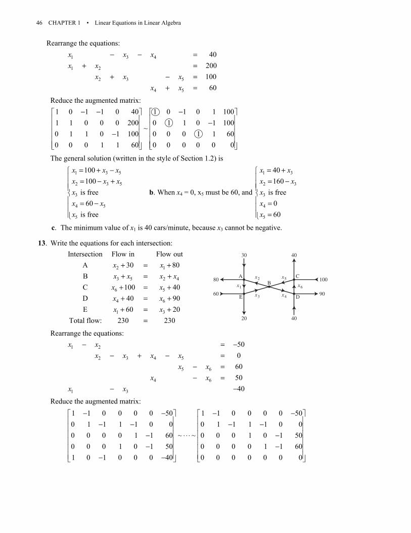
46 CHAPTER 1 • Linear Equations in Linear Algebra
Rearrange the equations:
1 3 4
1 2
2 3 5
4 5
40200100
60
x x xx x
x x xx x
− − =+ =
+ − =+ =
Reduce the augmented matrix:
1 0 1 1 0 40 1 0 1 0 1 1001 1 0 0 0 200 0 1 1 0 1 100
~0 1 1 0 1 100 0 0 0 1 1 600 0 0 1 1 60 0 0 0 0 0 0
− − − − −
The general solution (written in the style of Section 1.2) is
1 3 5
2 3 5
3
4 5
5
100100
is free60
is free
x x xx x xxx xx
= + − = − + = −
b. When x4 = 0, x5 must be 60, and
1 3
2 3
3
4
5
40160
is free060
x xx xxxx
= + = − =
=
c. The minimum value of x1 is 40 cars/minute, because x3 cannot be negative.
13. Write the equations for each intersection:
2 1
3 5 2 4
6 5
4 6
1 3
Intersection Flow in Flow outA 30 80BC 100 40D 40 90E 60 20
Total flow: 230 230
x xx x x x
x xx xx x
+ = ++ = ++ = ++ = ++ = +
=
Rearrange the equations:
1 2
2 3 4 5
5 6
4 6
1 3
500
605040
x xx x x x
x xx x
x x
− = −− + − =
− =− =
− −
Reduce the augmented matrix:
1 1 0 0 0 0 50 1 1 0 0 0 0 500 1 1 1 1 0 0 0 1 1 1 1 0 0
~ ~0 0 0 0 1 1 60 0 0 0 1 0 1 500 0 0 1 0 1 50 0 0 0 0 1 1 601 0 1 0 0 0 40 0 0 0 0 0 0 0
− − − − − − − − ⋅ ⋅ ⋅− − − − − −
60
80
90
100x1 x6
x2
x3
x5
x4
20 40
30 40
A
E
C
D
B

1.6 • Solutions 47
1 0 1 0 0 0 400 1 1 0 0 0 10
~ ~ 0 0 0 1 0 1 500 0 0 0 1 1 600 0 0 0 0 0 0
− − − ⋅ ⋅ ⋅ − −
a. The general solution is
1 3
2 3
3
4 6
5 6
6
4010
is free5060
is free
x xx xxx xx xx
= − = + = + = +
b. To find minimum flows, note that since x1 cannot be negative, x3 > 40. This implies that x2 > 50. Also, since x6 cannot be negative, x4 > 50 and x5 > 60. The minimum flows are x2 = 50, x3 = 40, x4 = 50, x5 = 60 (when x1 = 0 and x6 = 0).
14. Write the equations for each intersection.
1 2
2 3
3 4
4 5
5 6
6 1
Intersection Flow in Flow outA 100B 50C 120D 150E 80F 100
x xx x
x xx x
x xx x
= ++ =
= ++ =
= ++ =
Rearrange the equations:
1 2
2 3
3 4
4 5
5 6
1 6
10050
120150
80100
x xx x
x xx x
x xx x
− =− = −
− =− = −
− =− + = −
Reduce the augmented matrix:
1 1 0 0 0 0 100 1 1 0 0 0 0 1000 1 1 0 0 0 50 0 1 1 0 0 0 500 0 1 1 0 0 120 0 0 1 1 0 0 120
~ ~0 0 0 1 1 0 150 0 0 0 1 1 0 1500 0 0 0 1 1 80 0 0 0 0 1 1 801 0 0 0 0 1 100 0 0 0 0 0 0 0
− − − − − − − −
⋅⋅ ⋅ − − − − − − − −
100
50
x3
80
100
120 150
x2
x1
x6
x5x4
A
B E
F
C D

48 CHAPTER 1 • Linear Equations in Linear Algebra
1 0 0 0 0 1 1000 1 0 0 0 1 00 0 1 0 0 1 50
~ ~0 0 0 1 0 1 700 0 0 0 1 1 800 0 0 0 0 0 0
− − −
⋅⋅ ⋅ − − −
. The general solution is
1 6
2 6
3 6
4 6
5 6
6
100
5070
80 is free
x xx xx xx xx xx
= + = = + = − + = +
.
Since x4 cannot be negative, the minimum value of x6 is 70.
Note: The MATLAB box in the Study Guide discusses rational calculations, needed for balancing the chemical equations in Exercises 9 and 10. As usual, the appendices cover this material for Maple, Mathematica, and the TI and HP graphic calculators.
1.7 SOLUTIONS
Note: Key exercises are 9–20 and 23–30. Exercise 30 states a result that could be a theorem in the text. There is a danger, however, that students will memorize the result without understanding the proof, and then later mix up the words row and column. Exercises 37 and 38 anticipate the discussion in Section 1.9 of one-to-one transformations. Exercise 44 is fairly difficult for my students.
1. Use an augmented matrix to study the solution set of x1u + x2v + x3w = 0 (*), where u, v, and w are the
three given vectors. Since 5 7 9 0 5 7 9 00 2 4 0 ~ 0 2 4 00 6 8 0 0 0 4 0
− −
, there are no free variables. So the
homogeneous equation (*) has only the trivial solution. The vectors are linearly independent.
2. Use an augmented matrix to study the solution set of x1u + x2v + x3w = 0 (*), where u, v, and w are the
three given vectors. Since 0 0 3 0 2 8 1 00 5 4 0 ~ 0 5 4 02 8 1 0 0 0 3 0
− − − −
, there are no free variables. So the
homogeneous equation (*) has only the trivial solution. The vectors are linearly independent.
3. Use the method of Example 3 (or the box following the example). By comparing entries of the vectors, one sees that the second vector is –3 times the first vector. Thus, the two vectors are linearly dependent.
4. From the first entries in the vectors, it seems that the second vector of the pair 1 2
,4 8
− − −
may be 2
times the first vector. But there is a sign problem with the second entries. So neither of the vectors is a multiple of the other. The vectors are linearly independent.
5. Use the method of Example 2. Row reduce the augmented matrix for Ax = 0:
0 8 5 0 1 3 2 0 1 3 2 0 1 3 2 0 1 3 2 03 7 4 0 3 7 4 0 0 2 2 0 0 2 2 0 0 2 2 0
~ ~ ~ ~1 5 4 0 1 5 4 0 0 2 2 0 0 0 0 0 0 0 3 01 3 2 0 0 8 5 0 0 8 5 0 0 0 3 0 0 0 0 0
− − − − − − − − − − − − − − − − − − − −

1.7 • Solutions 49
There are no free variables. The equation Ax = 0 has only the trivial solution and so the columns of A are linearly independent.
6. Use the method of Example 2. Row reduce the augmented matrix for Ax = 0:
4 3 0 0 1 0 3 0 1 0 3 0 1 0 3 0 1 0 3 00 1 4 0 0 1 4 0 0 1 4 0 0 1 4 0 0 1 4 0
~ ~ ~ ~1 0 3 0 4 3 0 0 0 3 12 0 0 0 0 0 0 0 7 05 4 6 0 5 4 6 0 0 4 9 0 0 0 7 0 0 0 0 0
− − − − − − − − − − −
There are no free variables. The equation Ax = 0 has only the trivial solution and so the columns of A are linearly independent.
7. Study the equation Ax = 0. Some people may start with the method of Example 2:
1 4 3 0 0 1 4 3 0 0 1 4 3 0 02 7 5 1 0 ~ 0 1 1 1 0 ~ 0 1 1 1 04 5 7 5 0 0 11 5 5 0 0 0 6 6 0
− − − − − − − − − − −
But this is a waste of time. There are only 3 rows, so there are at most three pivot positions. Hence, at least one of the four variables must be free. So the equation Ax = 0 has a nontrivial solution and the columns of A are linearly dependent.
8. Same situation as with Exercise 7. The (unnecessary) row operations are
1 3 3 2 0 1 3 3 2 0 1 3 3 2 03 7 1 2 0 ~ 0 2 8 4 0 ~ 0 2 8 4 00 1 4 3 0 0 1 4 3 0 0 0 0 1 0
− − − − − − − − − − − − − −
Again, because there are at most three pivot positions yet there are four variables, the equation Ax = 0 has a nontrivial solution and the columns of A are linearly dependent.
9. a. The vector v3 is in Span{v1, v2} if and only if the equation x1v1 + x2v2 = v3 has a solution. To find out, row reduce [v1 v2 v3], considered as an augmented matrix:
1 3 5 1 3 53 9 7 ~ 0 0 82 6 0 0 10h h
− − − − − −
At this point, the equation 0 = 8 shows that the original vector equation has no solution. So v3 is in Span{v1, v2} for no value of h.
b. For {v1, v2, v3} to be linearly independent, the equation x1v1 + x2v2 + x3v3 = 0 must have only the trivial solution. Row reduce the augmented matrix [v1 v2 v3 0]
1 3 5 0 1 3 5 0 1 3 5 03 9 7 0 ~ 0 0 8 0 ~ 0 0 8 02 6 0 0 0 10 0 0 0 0 0h h
− − − − − − −
For every value of h, x2 is a free variable, and so the homogeneous equation has a nontrivial solution. Thus {v1, v2, v3} is a linearly dependent set for all h.

50 CHAPTER 1 • Linear Equations in Linear Algebra
10. a. The vector v3 is in Span{v1, v2} if and only if the equation x1v1 + x2v2 = v3 has a solution. To find out, row reduce [v1 v2 v3], considered as an augmented matrix:
1 2 2 1 2 25 10 9 ~ 0 0 13 6 0 0 6h h
− − − − − +
At this point, the equation 0 = 1 shows that the original vector equation has no solution. So v3 is in Span{v1, v2} for no value of h.
b. For {v1, v2, v3} to be linearly independent, the equation x1v1 + x2v2 + x3v3 = 0 must have only the trivial solution. Row reduce the augmented matrix [v1 v2 v3 0]
1 2 2 0 1 2 2 0 1 2 2 05 10 9 0 ~ 0 0 1 0 ~ 0 0 1 03 6 0 0 0 6 0 0 0 0 0h h
− − − − − − +
For every value of h, x2 is a free variable, and so the homogeneous equation has a nontrivial solution. Thus {v1, v2, v3} is a linearly dependent set for all h.
11. To study the linear dependence of three vectors, say v1, v2, v3, row reduce the augmented matrix [v1 v2 v3 0]:
1 3 1 0 1 3 1 0 1 3 1 01 5 5 0 ~ 0 2 4 0 ~ 0 2 4 04 7 0 0 5 4 0 0 0 6 0h h h
− − − − − − − − + −
The equation x1v1 + x2v2 + x3v3 = 0 has a nontrivial solution if and only if h – 6 = 0 (which corresponds to x3 being a free variable). Thus, the vectors are linearly dependent if and only if h = 6.
12. To study the linear dependence of three vectors, say v1, v2, v3, row reduce the augmented matrix [v1 v2 v3 0]:
2 6 8 0 2 6 8 04 7 0 ~ 0 5 16 01 3 4 0 0 0 0 0
h h− −
− − + −
The equation x1v1 + x2v2 + x3v3 = 0 has a free variable and hence a nontrivial solution no matter what the value of h. So the vectors are linearly dependent for all values of h.
13. To study the linear dependence of three vectors, say v1, v2, v3, row reduce the augmented matrix [v1 v2 v3 0]:
1 2 3 0 1 2 3 05 9 0 ~ 0 1 15 03 6 9 0 0 0 0 0
h h− −
− − − −
The equation x1v1 + x2v2 + x3v3 = 0 has a free variable and hence a nontrivial solution no matter what the value of h. So the vectors are linearly dependent for all values of h.

1.7 • Solutions 51
14. To study the linear dependence of three vectors, say v1, v2, v3, row reduce the augmented matrix [v1 v2 v3 0]:
1 5 1 0 1 5 1 0 1 5 1 01 7 1 0 ~ 0 2 2 0 ~ 0 2 2 03 8 0 0 7 3 0 0 0 10 0h h h
− − − − − − + +
The equation x1v1 + x2v2 + x3v3 = 0 has a nontrivial solution if and only if h + 10 = 0 (which corresponds to x3 being a free variable). Thus, the vectors are linearly dependent if and only if h = –10.
15. The set is linearly dependent, by Theorem 8, because there are four vectors in the set but only two entries in each vector.
16. The set is linearly dependent because the second vector is 3/2 times the first vector.
17. The set is linearly dependent, by Theorem 9, because the list of vectors contains a zero vector.
18. The set is linearly dependent, by Theorem 8, because there are four vectors in the set but only two entries in each vector.
19. The set is linearly independent because neither vector is a multiple of the other vector. [Two of the entries in the first vector are – 4 times the corresponding entry in the second vector. But this multiple does not work for the third entries.]
20. The set is linearly dependent, by Theorem 9, because the list of vectors contains a zero vector.
21. a. False. A homogeneous system always has the trivial solution. See the box before Example 2. b. False. See the warning after Theorem 7. c. True. See Fig. 3, after Theorem 8. d. True. See the remark following Example 4.
22. a. True. See Fig. 1.
b. False. For instance, the set consisting of 1 22 and –43 6
−
is linearly dependent. See the warning after
Theorem 8. c. True. See the remark following Example 4. d. False. See Example 3(a).
23. * *
0 *0 0
24. * 0 0 0
, ,0 0 0 0 0 0
25.
* 00 0 0
and 0 0 0 00 0 0 0

52 CHAPTER 1 • Linear Equations in Linear Algebra
26.
* *0 *0 00 0 0
. The columns must linearly independent, by Theorem 7, because the first column is not
zero, the second column is not a multiple of the first, and the third column is not a linear combination of the preceding two columns (because a3 is not in Span{a1, a2}).
27. All five columns of the 7×5 matrix A must be pivot columns. Otherwise, the equation Ax = 0 would have a free variable, in which case the columns of A would be linearly dependent.
28. If the columns of a 5×7 matrix A span R5, then A has a pivot in each row, by Theorem 4. Since each pivot position is in a different column, A has five pivot columns.
29. A: any 3×2 matrix with two nonzero columns such that neither column is a multiple of the other. In this case the columns are linearly independent and so the equation Ax = 0 has only the trivial solution.
B: any 3×2 matrix with one column a multiple of the other.
30. a. n b. The columns of A are linearly independent if and only if the equation Ax = 0 has only the trivial
solution. This happens if and only if Ax = 0 has no free variables, which in turn happens if and only if every variable is a basic variable, that is, if and only if every column of A is a pivot column.
31. Think of A = [a1 a2 a3]. The text points out that a3 = a1 + a2. Rewrite this as a1 + a2 – a3 = 0. As a matrix equation, Ax = 0 for x = (1, 1, –1).
32. Think of A = [a1 a2 a3]. The text points out that a1 + 2a2 = a3. Rewrite this as a1 + 2a2 – a3 = 0. As a matrix equation, Ax = 0 for x = (1, 2, –1).
33. True, by Theorem 7. (The Study Guide adds another justification.)
34. True, by Theorem 9.
35. False. The vector v1 could be the zero vector.
36. False. Counterexample: Take v1, v2, and v4 all to be multiples of one vector. Take v3 to be not a multiple of that vector. For example,
1 2 3 4
1 2 1 41 2 0 4
, , ,1 2 0 41 2 0 4
= = = =
v v v v
37. True. A linear dependence relation among v1, v2, v3 may be extended to a linear dependence relation among v1, v2, v3, v4 by placing a zero weight on v4.
38. True. If the equation x1v1 + x2v2 + x3v3 = 0 had a nontrivial solution (with at least one of x1, x2, x3 nonzero), then so would the equation x1v1 + x2v2 + x3v3 + 0⋅v4 = 0. But that cannot happen because {v1, v2, v3, v4} is linearly independent. So {v1, v2, v3} must be linearly independent. This problem can also be solved using Exercise 37, if you know that the statement there is true.

1.7 • Solutions 53
39. If for all b the equation Ax = b has at most one solution, then take b = 0, and conclude that the equation Ax = 0 has at most one solution. Then the trivial solution is the only solution, and so the columns of A are linearly independent.
40. An m×n matrix with n pivot columns has a pivot in each column. So the equation Ax = b has no free variables. If there is a solution, it must be unique.
41. [M]
8 3 0 7 2 8 3 0 7 29 4 5 11 7 0 5/8 5 25/8 19 / 4
~6 2 2 4 4 0 1/ 4 2 5/ 4 5/ 25 1 7 0 10 0 7 /8 7 35/8 35/ 4
A
− − − − − − − = − − −
8 3 0 7 2 8 3 0 7 20 5/8 5 25/8 19 / 4 0 5/8 5 25/8 19 / 4
~ ~0 0 0 0 22 / 5 0 0 0 0 22 / 50 0 0 0 77 / 5 0 0 0 0 0
− − − − − −
The pivot columns of A are 1, 2, and 5. Use them to form
8 3 29 4 76 2 45 1 10
B
− − − = − −
.
Other likely choices use columns 3 or 4 of A instead of 2:
8 0 2 8 7 29 5 7 9 11 7
,6 2 4 6 4 45 7 10 5 0 10
− − − − − −
.
Actually, any set of three columns of A that includes column 5 will work for B, but the concepts needed to prove that are not available now. (Column 5 is not in the two-dimensional subspace spanned by the first four columns.)
42. [M]
12 10 6 3 7 10 12 10 6 3 7 107 6 4 7 9 5 0 1/ 6 1/ 2 21/ 4 59 /12 65/ 6
~ ~9 9 9 5 5 1 0 0 0 89 / 2 89 / 2 894 3 1 6 8 9 0 0 0 0 0 38 7 5 9 11 8 0 0 0 0 0 0
− − − − − − − − − ⋅ ⋅ ⋅− − − − − − − − − −
The pivot columns of A are 1, 2, 4, and 6. Use them to form
12 10 3 107 6 7 59 9 5 14 3 6 98 7 9 8
B
− − − = − − − − − −
.
Other likely choices might use column 3 of A instead of 2, and/or use column 5 instead of 4.

54 CHAPTER 1 • Linear Equations in Linear Algebra
43. [M] Make v any one of the columns of A that is not in B and row reduce the augmented matrix [B v]. The calculations will show that the equation Bx = v is consistent, which means that v is a linear combination of the columns of B. Thus, each column of A that is not a column of B is in the set spanned by the columns of B.
44. [M] Calculations made as for Exercise 43 will show that each column of A that is not a column of B is in the set spanned by the columns of B. Reason: The original matrix A has only four pivot columns. If one or more columns of A are removed, the resulting matrix will have at most four pivot columns. (Use exactly the same row operations on the new matrix that were used to reduce A to echelon form.) If v is a column of A that is not in B, then row reduction of the augmented matrix [B v] will display at most four pivot columns. Since B itself was constructed to have four pivot columns, adjoining v cannot produce a fifth pivot column. Thus the first four columns of [B v] are the pivot columns. This implies that the equation Bx = v has a solution.
Note: At the end of Section 1.7, the Study Guide has another note to students about “Mastering Linear Algebra Concepts.” The note describes how to organize a review sheet that will help students form a mental image of linear independence. The note also lists typical misuses of terminology, in which an adjective is applied to an inappropriate noun. (This is a major problem for my students.) I require my students to prepare a review sheet as described in the Study Guide, and I try to make helpful comments on their sheets. I am convinced, through personal observation and student surveys, that the students who prepare many of these review sheets consistently perform better than other students. Hopefully, these students will remember important concepts for some time beyond the final exam.
1.8 SOLUTIONS
Notes: The key exercises are 17–20, 25 and 31. Exercise 20 is worth assigning even if you normally assign only odd exercises. Exercise 25 (and 27) can be used to make a few comments about computer graphics, even if you do not plan to cover Section 2.6. For Exercise 31, the Study Guide encourages students not to look at the proof before trying hard to construct it. Then the Guide explains how to create the proof.
Exercises 19 and 20 provide a natural segue into Section 1.9. I arrange to discuss the homework on these exercises when I am ready to begin Section 1.9. The definition of the standard matrix in Section 1.9 follows naturally from the homework, and so I’ve covered the first page of Section 1.9 before students realize we are working on new material.
The text does not provide much practice determining whether a transformation is linear, because the time needed to develop this skill would have to be taken away from some other topic. If you want your students to be able to do this, you may need to supplement Exercises 29, 30, 32 and 33.
If you skip the concepts of one-to-one and “onto” in Section 1.9, you can use the result of Exercise 31 to show that the coordinate mapping from a vector space onto Rn (in Section 4.4) preserves linear independence and dependence of sets of vectors. (See Example 6 in Section 4.4.)
1. T(u) = Au = 2 0 1 20 2 3 6
= − − , T(v) =
2 0 20 2 2
a ab b
=
2. T(u) = Au =.5 0 0 1 .50 .5 0 0 00 0 .5 4 2
= − −
, T(v) = .5 0 0 .50 .5 0 .50 0 .5 .5
a ab bc c
=

1.8 • Solutions 55
3. [ ]1 0 2 1 1 0 2 1 1 0 2 12 1 6 7 ~ 0 1 2 5 ~ 0 1 2 53 2 5 3 0 2 1 0 0 0 5 10
A− − − − − −
= − − − − −
b
1 0 2 1 1 0 0 3 3
~ 0 1 2 5 ~ 0 1 0 1 1 ,0 0 1 2 0 0 1 2 2
− − =
x unique solution
4. [ ]1 3 2 6 1 3 2 6 1 3 2 60 1 4 7 ~ 0 1 4 7 ~ 0 1 4 73 5 9 9 0 4 15 27 0 0 1 1
A− − −
= − − − − − − − − − − −
b
1 3 0 4 1 0 0 5 5
~ 0 1 0 3 ~ 0 1 0 3 30 0 1 1 0 0 1 1 1
− − − − − = −
x , unique solution
5. [ ] 1 5 7 2 1 5 7 2 1 0 3 3~ ~
3 7 5 2 0 1 2 1 0 1 2 1A
− − − − − − = − −
b
Note that a solution is not 31
. To avoid this common error, write the equations:
1 3
2 3
3 32 1
x xx x
+ =+ =
and solve for the basic variables: 1 3
2 3
3
3 31 2
is free
x xx xx
= − = −
General solution 1 3
2 3 3
3 3
3 3 3 31 2 1 2
0 1
x xx x xx x
− − = = − = + −
x . For a particular solution, one might choose
x3 = 0 and 310
=
x .
6. [ ]
1 2 1 1 1 2 1 1 1 2 1 1 1 0 3 73 4 5 9 0 2 2 6 0 1 1 3 0 1 1 3
~ ~ ~0 1 1 3 0 1 1 3 0 0 0 0 0 0 0 03 5 4 6 0 1 1 3 0 0 0 0 0 0 0 0
A
− − − − = − − − − − −
b
1 3
2 3
3 73
x xx x
+ =+ =
. 1 3
2 3
3
7 33
is free
x xx xx
= − = −
General solution: 1 3
2 3 3
3 3
7 3 7 33 3 1
0 1
x xx x xx x
− − = = − = + −
x , one choice: 730
.

56 CHAPTER 1 • Linear Equations in Linear Algebra
7. a = 5; the domain of T is R5, because a 6×5 matrix has 5 columns and for Ax to be defined, x must be in R5. b = 6; the codomain of T is R6, because Ax is a linear combination of the columns of A, and each column of A is in R6.
8. A must have 5 rows and 4 columns. For the domain of T to be R4, A must have four columns so that Ax is defined for x in R4. For the codomain of T to be R5, the columns of A must have five entries (in which case A must have five rows), because Ax is a linear combination of the columns of A.
9. Solve Ax = 0. 1 4 7 5 0 1 4 7 5 0 1 4 7 5 00 1 4 3 0 ~ 0 1 4 3 0 ~ 0 1 4 3 02 6 6 4 0 0 2 8 6 0 0 0 0 0 0
− − − − − − − − − − − −
1 0 9 7 0
~ 0 1 4 3 00 0 0 0 0
− −
1 3 4
2 3 4
9 7 04 3 0
0 0
x x xx x x
− + =− + =
=,
1 3 4
2 3 4
3
4
9 74 3
is free is free
x x xx x xxx
= − = −
x =
1 3 4
2 3 43 4
3 3
4 4
9 7 9 74 3 4 3
1 00 1
x x xx x x
x xx xx x
− − − − = = +
10. Solve Ax = 0.
1 3 9 2 0 1 3 9 2 0 1 3 9 2 01 0 3 4 0 0 3 6 6 0 0 1 2 3 0
~ ~0 1 2 3 0 0 1 2 3 0 0 3 6 6 02 3 0 5 0 0 9 18 9 0 0 9 18 9 0
− − − − − − − −
1 3 9 2 0 1 3 9 0 0 1 0 3 0 00 1 2 3 0 0 1 2 0 0 0 1 2 0 0
~ ~ ~0 0 0 3 0 0 0 0 1 0 0 0 0 1 00 0 0 18 0 0 0 0 0 0 0 0 0 0 0
−
1 3
2 3
4
3 02 0
0
x xx x
x
+ =+ =
=
1 3
2 3
3
4
32
is free0
x xx xxx
= − = − =
3
33
3
3 32 2
10 0
xx
xx
− − − − = =
x
11. Is the system represented by [A b] consistent? Yes, as the following calculation shows.
1 4 7 5 1 1 4 7 5 1 1 4 7 5 10 1 4 3 1 ~ 0 1 4 3 1 ~ 0 1 4 3 12 6 6 4 0 0 2 8 6 2 0 0 0 0 0
− − − − − − − − − − − − − − −
The system is consistent, so b is in the range of the transformation Ax x .

1.8 • Solutions 57
12. Is the system represented by [A b] consistent?
1 3 9 2 1 1 3 9 2 1 1 3 9 2 11 0 3 4 3 0 3 6 6 4 0 1 2 3 1
~ ~0 1 2 3 1 0 1 2 3 1 0 3 6 6 42 3 0 5 4 0 9 18 9 2 0 9 18 9 2
− − − − − − − − − − − − − −
1 3 9 2 1 1 3 9 2 10 1 2 3 1 0 1 2 3 1
~ ~0 0 0 3 1 0 0 0 3 10 0 0 18 11 0 0 0 0 17
− − − − −
The system is inconsistent, so b is not in the range of the transformation Ax x .
13. 14.
x2
u
v
T(u)
T(v)
x1
x1
x2
u
v
T(v)
T(u)
A reflection through the origin. A contraction by the factor .5.
The transformation in Exercise 13 may also be described as a rotation of π radians about the origin or a rotation of –π radians about the origin.
15. 16.
x1
x2
u
v T(v)
T(u)
x1
x2
u
v
T(u)
T(v)
A projection onto the x2-axis A reflection through the line x2 = x1.
17. T(3u) = 3T(u) = 2 6
31 3
=
, T(2v) = 2T(v) =
1 22
3 6− −
=
, and
T(3u + 2v) = 3T(u) = 2T(v) = 6 2 43 6 9
− + =
.
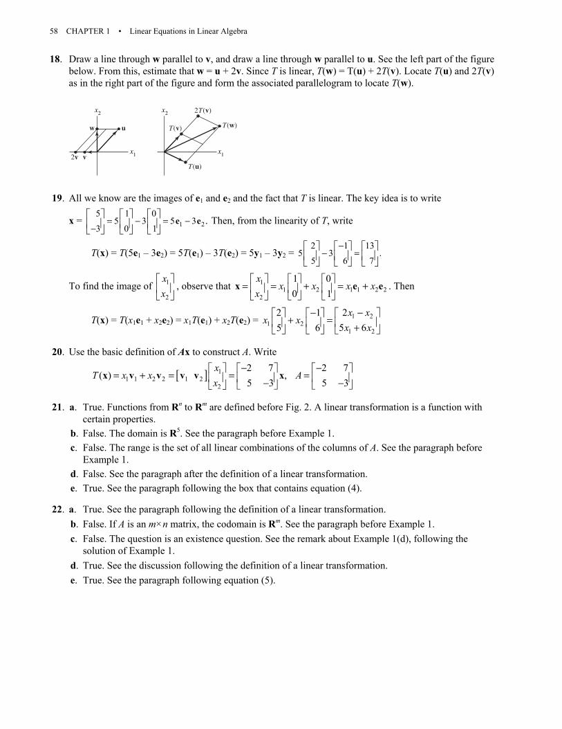
58 CHAPTER 1 • Linear Equations in Linear Algebra
18. Draw a line through w parallel to v, and draw a line through w parallel to u. See the left part of the figure below. From this, estimate that w = u + 2v. Since T is linear, T(w) = T(u) + 2T(v). Locate T(u) and 2T(v) as in the right part of the figure and form the associated parallelogram to locate T(w).
x1
x2
x1
x2
uw
v2v
T(v)
2T(v)
T(u)
T(w)
19. All we know are the images of e1 and e2 and the fact that T is linear. The key idea is to write
x = 1 25 1 0
5 3 5 33 0 1
.= − = −−
e e Then, from the linearity of T, write
T(x) = T(5e1 – 3e2) = 5T(e1) – 3T(e2) = 5y1 – 3y2 = 2 1 13
5 3 .5 6 7
−− =
To find the image of 1
2
xx
, observe that 11 2 1 1 2 2
2
1 00 1
xx x x x
x
= = + = +
x e e . Then
T(x) = T(x1e1 + x2e2) = x1T(e1) + x2T(e2) = 1 21 2
1 2
22 15 65 6
x xx x
x x−−
+ = +
20. Use the basic definition of Ax to construct A. Write
[ ] 11 1 2 2 1 2
2
2 7 2 7( ) ,
5 3 5 3x
T x x Ax
− − = + = = = − −
x v v v v x
21. a. True. Functions from Rn to Rm are defined before Fig. 2. A linear transformation is a function with certain properties.
b. False. The domain is R5. See the paragraph before Example 1. c. False. The range is the set of all linear combinations of the columns of A. See the paragraph before
Example 1. d. False. See the paragraph after the definition of a linear transformation. e. True. See the paragraph following the box that contains equation (4).
22. a. True. See the paragraph following the definition of a linear transformation. b. False. If A is an m×n matrix, the codomain is Rm. See the paragraph before Example 1. c. False. The question is an existence question. See the remark about Example 1(d), following the
solution of Example 1. d. True. See the discussion following the definition of a linear transformation. e. True. See the paragraph following equation (5).

1.8 • Solutions 59
23.
x1
x2
u
cu
T (cu)T(u)
T(u)
T(u + v)
u + v
x1
x2
T(v)
vu
24. Given any x in Rn, there are constants c1, …, cp such that x = c1v1 + ··· cpvp, because v1, …, vp span Rn. Then, from property (5) of a linear transformation,
T(x) = c1T(v1) + ··· + cpT(vp) = c10 + ·· + cp0 = 0
25. Any point x on the line through p in the direction of v satisfies the parametric equation x = p + tv for some value of t. By linearity, the image T(x) satisfies the parametric equation T(x) = T(p + tv) = T(p) + tT(v) (*) If T(v) = 0, then T(x) = T(p) for all values of t, and the image of the original line is just a single point.
Otherwise, (*) is the parametric equation of a line through T(p) in the direction of T(v).
26. Any point x on the plane P satisfies the parametric equation x = su + tv for some values of s and t. By linearity, the image T(x) satisfies the parametric equation
T(x) = sT(u) + tT(v) (s, t in R) (*) The set of images is just Span{T(u), T(v)}. If T(u) and T(v) are linearly independent, Span{T(u), T(v)} is
a plane through T(u), T(v), and 0. If T(u) and T(v) are linearly dependent and not both zero, then Span{T(u), T(v)} is a line through 0. If T(u) = T(v) = 0, then Span{T(u), T(v)} is {0}.
27. a. From Fig. 7 in the exercises for Section 1.5, the line through T(p) and T(q) is in the direction of q – p, and so the equation of the line is x = p + t(q – p) = p + tq – tp = (1 – t)p + tq.
b. Consider x = (1 – t)p + tq for t such that 0 < t < 1. Then, by linearity of T, T(x) = T((1 – t)p + tq) = (1 – t)T(p) + tT(q) 0 < t < 1 (*) If T(p) and T(q) are distinct, then (*) is the equation for the line segment between T(p) and T(q), as
shown in part (a) Otherwise, the set of images is just the single point T(p), because (1 – t)T(p) + tT(q) =(1 – t)T(p) + tT(p) = T(p)
28. Consider a point x in the parallelogram determined by u and v, say x = au + bv for 0 < a < 1, 0 < b < 1. By linearity of T, the image of x is
T(x) = T(au + bv) = aT(u) + bT(v), for 0 < a < 1, 0 < b < 1 (*) This image point lies in the parallelogram determined by T(u) and T(v). Special “degenerate” cases arise when T(u) and T(v) are linearly dependent. If one of the images is not
zero, then the “parallelogram” is actually the line segment from 0 to T(u) + T(v). If both T(u) and T(v) are zero, then the parallelogram is just {0}. Another possibility is that even u and v are linearly dependent, in which case the original parallelogram is degenerate (either a line segment or the zero vector). In this case, the set of images must be degenerate, too.
29. a. When b = 0, f (x) = mx. In this case, for all x,y in R and all scalars c and d, f (cx + dy) = m(cx + dy) = mcx + mdy = c(mx) + d(my) = c·f (x) + d·f (y) This shows that f is linear.

60 CHAPTER 1 • Linear Equations in Linear Algebra
b. When f (x) = mx + b, with b nonzero, f(0) = m(0) = b = b ≠ 0. This shows that f is not linear, because every linear transformation maps the zero vector in its domain into the zero vector in the codomain. (In this case, both zero vectors are just the number 0.) Another argument, for instance, would be to calculate f (2x) = m(2x) + b and 2f (x) = 2mx + 2b. If b is nonzero, then f (2x) is not equal to 2f (x) and so f is not a linear transformation.
c. In calculus, f is called a “linear function” because the graph of f is a line.
30. Let T(x) = Ax + b for x in Rn. If b is not zero, T(0) = A0 + b = b ≠ 0. Actually, T fails both properties of a linear transformation. For instance, T(2x) = A(2x) + b = 2Ax + b, which is not the same as 2T(x) = 2(Ax + b) = 2Ax + 2b. Also,
T(x + y) = A(x + y) + b = Ax + Ay + b which is not the same as T(x) + T(y) = Ax + b + Ay + b
31. (The Study Guide has a more detailed discussion of the proof.) Suppose that {v1, v2, v3} is linearly dependent. Then there exist scalars c1, c2, c3, not all zero, such that
c1v1 + c2v2 + c3v3 = 0 Then T(c1v1 + c2v2 + c3v3) = T(0) = 0. Since T is linear, c1T(v1) + c2T(v2) + c3T(v3) = 0 Since not all the weights are zero, {T(v1), T(v2), T(v3)} is a linearly dependent set.
32. Take any vector (x1, x2) with x2 ≠ 0, and use a negative scalar. For instance, T(0, 1) = (–2, 3), but T(–1·(0, 1)) = T(0, –1) = (2, 3) ≠ (–1)·T(0, 1).
33. One possibility is to show that T does not map the zero vector into the zero vector, something that every linear transformation does do. T(0, 0) = (0, 4, 0).
34. Suppose that {u, v} is a linearly independent set in Rn and yet T(u) and T(v) are linearly dependent. Then there exist weights c1, c2, not both zero, such that
c1T(u) + c2T(v) = 0 Because T is linear, T(c1u + c2v) = 0. That is, the vector x = c1u + c2v satisfies T(x) = 0. Furthermore,
x cannot be the zero vector, since that would mean that a nontrivial linear combination of u and v is zero, which is impossible because u and v are linearly independent. Thus, the equation T(x) = 0 has a nontrivial solution.
35. Take u and v in R3 and let c and d be scalars. Then cu + dv = (cu1 + dv1, cu2 + dv2, cu3 + dv3). The transformation T is linear because T(cu + dv) = (cu1 + dv1, cu2 + dv2, – (cu3 + dv3)) = (cu1 + dv1, cu2 + dv2, cu3 dv3) = (cu1, cu2, cu3) + (dv1, dv2, dv3) = c(u1, u2, u3) + d(v1, v2, v3) = cT(u) + dT(v)
36. Take u and v in R3 and let c and d be scalars. Then cu + dv = (cu1 + dv1, cu2 + dv2, cu3 + dv3). The transformation T is linear because T(cu + dv) = (cu1 + dv1, 0, cu3 + dv3) = (cu1, 0, cu3) + (dv1, 0, dv3) = c(u1, 0, u3) + d(v1, 0, v3) = cT(u) + dT(v)

1.8 • Solutions 61
37. [M]
4 2 5 5 0 1 0 0 7 / 2 09 7 8 0 0 0 1 0 9 / 2 0
~ ,6 4 5 3 0 0 0 1 0 05 3 8 4 0 0 0 0 0 0
− − − − − − − − −
1 4
2 4
3
4
(7 / 2)(9 / 2)0
is free
x xx xxx
= = =
4
7 / 29 / 2
01
x
=
x
38. [M]
9 4 9 4 0 1 0 0 3/ 4 05 8 7 6 0 0 1 0 5/ 4 0
~7 11 16 9 0 0 0 1 7 / 4 09 7 4 5 0 0 0 0 0 0
− − − − − − − − −
,
1 4
2 4
3 4
4
(3/ 4)(5/ 4)
(7 / 4) is free
x xx xx xx
= − = − =
4
3/ 45/ 4
7 / 41
x
− − =
x
39. [M]
4 2 5 5 7 1 0 0 7 / 2 49 7 8 0 5 0 1 0 9 / 2 7
~6 4 5 3 9 0 0 1 0 15 3 8 4 7 0 0 0 0 0
− − − − − − − − −
, yes, b is in the range of the transformation,
because the augmented matrix shows a consistent system. In fact,
the general solution is
1 4
2 4
3
4
4 (7 / 2)7 (9 / 2)1
is free
x xx xxx
= + = + =
; when x4 = 0 a solution is
4710
=
x .
40. [M]
9 4 9 4 7 1 0 0 3/ 4 5/ 45 8 7 6 7 0 1 0 5/ 4 11/ 4
~7 11 16 9 13 0 0 1 7 / 4 13/ 49 7 4 5 5 0 0 0 0 0
− − − − − − − − − − − − − −
, yes, b is in the range of the
transformation, because the augmented matrix shows a consistent system. In fact,
the general solution is
1 4
2 4
3 4
4
5 / 4 (3/ 4)11/ 4 (5/ 4)
13/ 4 (7 / 4) is free
x xx xx xx
= − − = − − = +
; when x4 = 1 a solution is
2451
− − =
x .
Notes: At the end of Section 1.8, the Study Guide provides a list of equations, figures, examples, and connections with concepts that will strengthen a student’s understanding of linear transformations. I encourage my students to continue the construction of review sheets similar to those for “span” and “linear independence,” but I refrain from collecting these sheets. At some point the students have to assume the responsibility for mastering this material.
If your students are using MATLAB or another matrix program, you might insert the definition of matrix multiplication after this section, and then assign a project that uses random matrices to explore properties of matrix multiplication. See Exercises 34–36 in Section 2.1. Meanwhile, in class you can continue with your plans for finishing Chapter 1. When you get to Section 2.1, you won’t have much to do. The Study Guide’s MATLAB note for Section 2.1 contains the matrix notation students will need for a project on matrix multiplication. The appendices in the Study Guide have the corresponding material for Mathematica, Maple, and the T-83+/86/89 and HP-48G graphic calculators.

62 CHAPTER 1 • Linear Equations in Linear Algebra
1.9 SOLUTIONS
Notes: This section is optional if you plan to treat linear transformations only lightly, but many instructors will want to cover at least Theorem 10 and a few geometric examples. Exercises 15 and 16 illustrate a fast way to solve Exercises 17–22 without explicitly computing the images of the standard basis.
The purpose of introducing one-to-one and onto is to prepare for the term isomorphism (in Section 4.4) and to acquaint math majors with these terms. Mastery of these concepts would require a substantial digression, and some instructors prefer to omit these topics (and Exercises 25–40). In this case, you can use the result of Exercise 31 in Section 1.8 to show that the coordinate mapping from a vector space onto Rn (in Section 4.4) preserves linear independence and dependence of sets of vectors. (See Example 6 in Section 4.4.) The notions of one-to-one and onto appear in the Invertible Matrix Theorem (Section 2.3), but can be omitted there if desired
Exercises 25–28 and 31–36 offer fairly easy writing practice. Exercises 31, 32, and 35 provide important links to earlier material.
1. A = [T(e1) T(e2)] =
3 51 23 01 0
−
2. A = [T(e1) T(e2) T(e3)] = 1 4 53 7 4
− −
3. T(e1) = –e2, T(e2) = e1. A = [ ]2 10 11 0
− = −
e e
4. T(e1) = 1/ 2
1/ 2
−
, T(e2) = 1/ 2
1/ 2
, A = 1/ 2 1/ 2
1/ 2 1/ 2
−
5. T(e1) = e1 – 2e2 = 12
−
, T(e2) = e2, A = 1 02 1
−
6. T(e1) = e1, T(e2) = e2 + 3e1 = 31
, A = 1 30 1
7. Follow what happens to e1 and e2. Since e1 is on the unit circle in the plane, it rotates through –3 /4π radians into a point on the unit circle that lies in the third quadrant and on the line 2 1x x= (that is, y x= in more familiar notation). The point (–1,–1) is on the ine 2 1x x= , but its distance from the origin is 2. So the rotational image of e1 is (–1/ 2, –1/ 2) . Then this image reflects in the horizontal axis to (–1/ 2,1/ 2) .
Similarly, e2 rotates into a point on the unit circle that lies in the second quadrant and on the line 2 1x x= , namely,

1.9 • Solutions 63
(–1/ 2, –1/ 2) . Then this image reflects in the horizontal axis to (–1/ 2,1/ 2) .
When the two calculations described above are written in vertical vector notation, the transformation’s standard matrix [T(e1) T(e2)] is easily seen:
1 21/ 2 1/ 2 1/ 2 1/ 2
,1/ 2 1/ 2 1/ 2 1/ 2
− −→ → → →
− − e e ,
1/ 2 1/ 2
1/ 2 1/ 2A
−=
8. [ ]1 1 2 2 2 1 2 10 1
and , so 1 0
A−
→ → → − → − = − =
e e e e e e e e
9. The horizontal shear maps e1 into e1, and then the reflection in the line x2 = –x1 maps e1 into –e2. (See Table 1.) The horizontal shear maps e2 into e2 into e2 – 2e1. To find the image of e2 – 2e1 when it is reflected in the line x2 = –x1, use the fact that such a reflection is a linear transformation. So, the image of e2 – 2e1 is the same linear combination of the images of e2 and e1, namely, –e1 – 2(–e2) = – e1 + 2e2. To summarize,
1 1 2 2 2 1 1 20 1
and 2 2 , so 1 2
A−
→ → − → − → − + = − e e e e e e e e
To find the image of e2 – 2e1 when it is reflected through the vertical axis use the fact that such a reflection is a linear transformation. So, the image of e2 – 2e1 is the same linear combination of the images of e2 and e1, namely, e2 + 2e1.
10. 1 1 2 2 2 1 ,0 1
and so1 0
A→ → → →−
− − − = − e e e e e e
11. The transformation T described maps 1 1 1→ → −e e e and maps 2 2 2.→ − → −e e e A rotation through π radians also maps e1 into –e1 and maps e2 into –e2. Since a linear transformation is completely determined by what it does to the columns of the identity matrix, the rotation transformation has the same effect as T on every vector in 2.R
12. The transformation T in Exercise 8 maps 1 1 2→ →e e e and maps 2 2 1→ − → −e e e . A rotation about the origin through / 2π radians also maps e1 into e2 and maps e2 into –e1. Since a linear transformation is completely determined by what it does to the columns of the identity matrix, the rotation transformation has the same effect as T on every vector in 2.R
13. Since (2, 1) = 2e1 + e2, the image of (2, 1) under T is 2T(e1) + T(e2), by linearity of T. On the figure in the exercise, locate 2T(e1) and use it with T(e2) to form the parallelogram shown below.
x1
x2
T(e2)2T(e1)
T(e1)
T(2, 1)

64 CHAPTER 1 • Linear Equations in Linear Algebra
14. Since T(x) = Ax = [a1 a2]x = x1a1 + x2a2 = –a1 + 3a2, when x = (–1, 3), the image of x is located by forming the parallelogram shown below.
x1
x2
T(–1, 3)
a2
a1
–a1
15. By inspection, 1 1 3
2 1
3 1 2 3
3 0 2 3 24 0 0 41 1 1
x x xx xx x x x
− − = − − +
16. By inspection, 1 2
11 2
21
1 12 1 21 0
x xx
x xx
x
− − − = − +
17. To express T(x) as Ax , write T(x) and x as column vectors, and then fill in the entries in A by inspection, as done in Exercises 15 and 16. Note that since T(x) and x have four entries, A must be a 4×4 matrix.
T(x) =
1 1
1 2 2 2
2 3 3 3
3 4 4 4
0 0 0 0 01 1 0 00 1 1 00 0 1 1
x xx x x x
Ax x x xx x x x
+ = = + +
18. As in Exercise 17, write T(x) and x as column vectors. Since x has 2 entries, A has 2 columns. Since T(x) has 4 entries, A has 4 rows.
2 1
1 2 1 1
2 2
2
2 3 3 24 1 4
0 0 00 1
x xx x x x
Ax x
x
− − − − = =
19. Since T(x) has 2 entries, A has 2 rows. Since x has 3 entries, A has 3 columns.
1 1
1 2 32 2
2 33 3
5 4 1 5 46 0 1 6
x xx x x
A x xx x
x x
− + − = = − −
20. Since T(x) has 1 entry, A has 1 row. Since x has 4 entries, A has 4 columns.
1 1
2 21 3 4
3 3
4 4
[2 3 4 ] [ ] [2 0 3 4]
x xx x
x x x Ax xx x
+ − = = −

1.9 • Solutions 65
21. T(x) = 1 2 1 1
1 2 2 2
1 14 5 4 5
x x x xA
x x x x+
= = + . To solve T(x) =
38
, row reduce the augmented matrix:
1 1 3 1 1 3 1 0 7 7~ ~ ,
4 5 8 0 1 4 0 1 4 4
= − − − x .
22. T(x) = 1 2
1 11 2
2 21 2
2 1 23 1 3
3 2 3 2
x xx x
x x Ax x
x x
− − − + = = − − −
. To solve T(x) = 149
−
, row reduce the augmented
matrix:
1 2 1 1 2 1 1 2 1 1 0 51 3 4 ~ 0 1 3 ~ 0 1 3 ~ 0 1 33 2 9 0 4 12 0 0 0 0 0 0
− − − − − − − −
, 5
.3
=
x
23. a. True. See Theorem 10. b. True. See Example 3. c. False. See the paragraph before Table 1. d. False. See the definition of onto. Any function from Rn to Rm maps each vector onto another vector. e. False. See Example 5.
24. a. False. See the paragraph preceding Example 2. b. True. See Theorem 10. c. True. See Table 1. d. False. See the definition of one-to-one. Any function from Rn to Rm maps a vector onto a single
(unique) vector. e. True. See the solution of Example 5.
25. Three row interchanges on the standard matrix A of the transformation T in Exercise 17 produce 1 1 0 00 1 1 00 0 1 10 0 0 0
. This matrix shows that A has only three pivot positions, so the equation Ax = 0 has a
nontrivial solution. By Theorem 11, the transformation T is not one-to-one. Also, since A does not have a pivot in each row, the columns of A do not span R4. By Theorem 12, T does not map R4 onto R4.
26. The standard matrix A of the transformation T in Exercise 2 is 2×3. Its columns are linearly dependent because A has more columns than rows. So T is not one-to-one, by Theorem 12. Also, A is row
equivalent to 1 4 50 19 19
− −
, which shows that the rows of A span R2. By Theorem 12, T maps R3
onto R2.
27. The standard matrix A of the transformation T in Exercise 19 is 1 5 40 1 6
− −
. The columns of A are
linearly dependent because A has more columns than rows. So T is not one-to-one, by Theorem 12. Also, A has a pivot in each row, so the rows of A span R2. By Theorem 12, T maps R3 onto R2.

66 CHAPTER 1 • Linear Equations in Linear Algebra
28. The standard matrix A of the transformation T in Exercise 14 has linearly independent columns, because the figure in that exercise shows that a1 and a2 are not multiples. So T is one-to-one, by Theorem 12. Also, A must have a pivot in each column because the equation Ax = 0 has no free variables. Thus, the
echelon form of A is *
0.
Since A has a pivot in each row, the columns of A span R2. So T maps R2
onto R2. An alternate argument for the second part is to observe directly from the figure in Exercise 14 that a1 and a2 span R2. This is more or less evident, based on experience with grids such as those in Figure 8 and Exercise 7 of Section 1.3.
29. By Theorem 12, the columns of the standard matrix A must be linearly independent and hence the
equation Ax = 0 has no free variables. So each column of A must be a pivot column:
* *0 *
~ .0 00 0 0
A
Note that T cannot be onto because of the shape of A.
30. By Theorem 12, the columns of the standard matrix A must span R3. By Theorem 4, the matrix must
have a pivot in each row. There are four possibilities for the echelon form:
* * * * * * * * * 0 * *
0 * * , 0 * * , 0 0 * , 0 0 *0 0 * 0 0 0 0 0 0 0 0 0
Note that T cannot be one-to-one because of the shape of A.
31. “T is one-to-one if and only if A has n pivot columns.” By Theorem 12(b), T is one-to-one if and only if the columns of A are linearly independent. And from the statement in Exercise 30 in Section 1.7, the columns of A are linearly independent if and only if A has n pivot columns.
32. The transformation T maps Rn onto Rm if and only if the columns of A span Rm, by Theorem 12. This happens if and only if A has a pivot position in each row, by Theorem 4 in Section 1.4. Since A has m rows, this happens if and only if A has m pivot columns. Thus, “T maps Rn onto Rm if and only A has m pivot columns.”
33. Define : n mT →R R by T(x) = Bx for some m×n matrix B, and let A be the standard matrix for T. By definition, A = [T(e1) ⋅ ⋅ ⋅ T(en)], where ej is the jth column of In. However, by matrix-vector multiplication, T(ej) = Bej = bj, the jth column of B. So A = [b1 ⋅ ⋅ ⋅ bn] = B.
34. The transformation T maps Rn onto Rm if and only if for each y in Rm there exists an x in Rn such that y = T(x).
35. If : n mT →R R maps nR onto mR , then its standard matrix A has a pivot in each row, by Theorem 12 and by Theorem 4 in Section 1.4. So A must have at least as many columns as rows. That is, m < n. When T is one-to-one, A must have a pivot in each column, by Theorem 12, so m > n.
36. Take u and v in Rp and let c and d be scalars. Then T(S(cu + dv)) = T(c⋅S(u) + d⋅S(v)) because S is linear = c⋅T(S(u)) + d⋅T(S(v)) because T is linear This calculation shows that the mapping x → T(S(x)) is linear. See equation (4) in Section 1.8.

1.10 • Solutions 67
37. [M]
5 10 5 4 1 0 0 44 / 35 1 0 0 1.25718 3 4 7 0 1 0 79 / 35 0 1 0 2.2571
~ ~ ~4 9 5 3 0 0 1 86 / 35 0 0 1 2.45713 2 5 4 0 0 0 0 0 0 0 0
− − − ⋅ ⋅ ⋅ − − − −
. There is no pivot in the
fourth column of the standard matrix A, so the equation Ax = 0 has a nontrivial solution. By Theorem 11, the transformation T is not one-to-one. (For a shorter argument, use the result of Exercise 31.)
38. [M]
7 5 4 9 1 0 7 010 6 16 4 0 1 9 0
~ ~12 8 12 7 0 0 0 1
8 6 2 5 0 0 0 0
− − − ⋅ ⋅ ⋅ − − −
. No. There is no pivot in the third column of the
standard matrix A, so the equation Ax = 0 has a nontrivial solution. By Theorem 11, the transformation T is not one-to-one. (For a shorter argument, use the result of Exercise 31.)
39. [M]
4 7 3 7 5 1 0 0 5 06 8 5 12 8 0 1 0 1 0
~ ~7 10 8 9 14 0 0 1 2 03 5 4 2 6 0 0 0 0 15 6 6 7 3 0 0 0 0 0
− − − ⋅ ⋅ ⋅− − − − − − − − −
. There is not a pivot in every row, so
the columns of the standard matrix do not span R5. By Theorem 12, the transformation T does not map R5 onto R5.
40. [M]
9 13 5 6 1 1 0 0 0 514 15 7 6 4 0 1 0 0 4
~ ~8 9 12 5 9 0 0 1 0 05 6 8 9 8 0 0 0 1 1
13 14 15 2 11 0 0 0 0 0
− − − − ⋅ ⋅ ⋅− − − − − − −
. There is not a pivot in every row, so
the columns of the standard matrix do not span R5. By Theorem 12, the transformation T does not map R5 onto R5.
1.10 SOLUTIONS
1. a. If x1 is the number of servings of Cheerios and x2 is the number of servings of 100% Natural Cereal, then x1 and x2 should satisfy
1 2
nutrients nutrients quantitiesper serving per serving of of nutrientsof Cheerios 100% Natural required
x x
+ =
That is,
1 2
110 130 2954 3 9
20 18 482 5 8
x x
+ =

68 CHAPTER 1 • Linear Equations in Linear Algebra
b. The equivalent matrix equation is 1
2
110 130 2954 3 9
20 18 482 5 8
xx
=
. To solve this, row reduce the augmented
matrix for this equation.
110 130 295 2 5 8 1 2.5 44 3 9 4 3 9 4 3 9
~ ~20 18 48 20 18 48 10 9 24
2 5 8 110 130 295 110 130 295
1 2.5 4 1 2.5 4 1 0 1.50 7 7 0 1 1 0 1 1
~ ~ ~0 16 16 0 0 0 0 0 00 145 145 0 0 0 0 0 0
− − − − − −
The desired nutrients are provided by 1.5 servings of Cheerios together with 1 serving of 100% Natural Cereal.
2. Set up nutrient vectors for one serving of Kellogg’s Cracklin’ Oat Bran (COB) and Kellogg's Crispix (Crp):
Nutrients: COB Crp
calories 110 110protein 3 2carbohydrate 21 25fat 3 .4
.
a. Let [ ]
110 1103 2 3
COB Crp ,21 25 23 .4
B
= = =
u .
Then Bu lists the amounts of calories, protein, carbohydrate, and fat in a mixture of three servings of Cracklin' Oat Bran and two servings of Crispix.
b. Let u1 and u2 be the number of servings of Cracklin’ Oat Bran and Crispix, respectively. Can these
numbers satisfy the equation 1
2
1102.25241
Buu
=
? To find out, row reduce the augmented matrix
110 110 110 1 1 1 1 1 1 1 1 13 2 2.25 3 2 2.25 0 1 .75 0 1 .75
~ ~ ~21 25 24 21 25 24 0 4 3 0 0 03 .4 1 3 .4 1 0 2.6 2 0 0 .05
− − − − − − −

1.10 • Solutions 69
The last row identifies an inconsistent system, because 0 = –.05 is impossible. So, technically, there is no mixture of the two cereals that will supply exactly the desired list of nutrients. However, one could tentatively ignore the final equation and see what the other equations prescribe. They reduce to u1 = .25 and u2 = .75. What does the corresponding mixture provide?
COB + Crp =
110 110 1103 2 2.25
.25 .75 .25 .7521 25 243 .4 1.05
⋅ ⋅ + =
The error of 5% for fat might be acceptable for practical purposes. Actually, the data in COB and Crp are certainly not precise and may have some errors even greater than 5%.
3. Here are the data, assembled from Table 1 and Exercise 3:
Mg of Nutrients/Unit NutrientsRequiredsoy soyNutrient (milligrams)milk flour whey prot.
protein 36 51 13 80 33carboh. 52 34 74 0 45fat 0 7 1.1 3.4 3calcium 1.26 .19 .8 .18 .8
a. Let x1, x2, x3, x4 represent the number of units of nonfat milk, soy flour, whey, and isolated soy protein, respectively. These amounts must satisfy the following matrix equation
1
2
3
4
36 51 13 80 3352 34 74 0 450 7 1.1 3.4 3
1.26 .19 .8 .18 .8
xxxx
=
b. [M]
36 51 13 80 33 0 0 0 .64152 34 74 0 45 0 0 0 .541~ ~0 7 1.1 3.4 3 0 0 0 .091
1.26 .19 .8 .18 .8 0 0 0 .211
⋅ ⋅ ⋅ − −
The “solution” is x1 = .64, x2 = .54, x3 = –.09, x4 = –.21. This solution is not feasible, because the mixture cannot include negative amounts of whey and isolated soy protein. Although the coefficients of these two ingredients are fairly small, they cannot be ignored. The mixture of .64 units of nonfat milk and .54 units of soy flour provide 50.6 g of protein, 51.6 g of carbohydrate, 3.8 g of fat, and .9 g of calcium. Some of these nutrients are nowhere close to the desired amounts.
4. Let x1, x2, and x3 be the number of units of foods 1, 2, and 3, respectively, needed for a meal. The values of x1, x2, and x3 should satisfy
1 2 3
nutrients nutrients nutrients milligrams(in mg) (in mg) (in mg) of nutrientsper unit per unit per unit requiredof Food 1 of Food 2 of Food 3x x x + + =

70 CHAPTER 1 • Linear Equations in Linear Algebra
From the given data,
1 2 3
10 20 20 100
50 40 10 300
30 10 40 200
x x x + + =
To solve, row reduce the corresponding augmented matrix:
10 20 20 100 10 20 20 100 1 2 2 1050 40 10 300 ~ 0 60 90 200 ~ 0 1 3/ 2 10 / 330 10 40 200 0 50 20 100 0 5 2 10
− − − − − −
1 2 2 10 1 2 0 250 / 33 1 0 0 50 /11
~ 0 1 3/ 2 10 / 3 ~ 0 1 0 50 / 33 ~ 0 1 0 50 / 330 0 1 40 / 33 0 0 1 40 / 33 0 0 1 40 /33
50 /11 4.55 units of Food 150 / 33 1.52 units of Food 240 / 33 1.21 units of Food 3
= = =
x
5. Loop 1: The resistance vector is
1
2 21
3
4
Total of four RI voltage drops for current 5Voltage drop for is negative; flows in opposite direction2Current does not flow in loop 10Current does not flow in loop 10
II I
II
− =
r
Loop 2: The resistance vector is
1 1
22
3 3
2 Voltage drop for is negative; flows in opposite direction11 Total of four RI voltage drops for current
Voltage drop for is negative; flows in opposite direction3Current0
I II
I I
− = −
r
4 does not flow in loop 2I
Also, r3 =
03
174
− −
, r4 =
004
25
−
, and R = [r1 r2 r3 r4] =
5 0 023 02 11
0 3 17 40 0 254
−
−− − − −
.
Notice that each off-diagonal entry of R is negative (or zero). This happens because the loop current directions are all chosen in the same direction on the figure. (For each loop j, this choice forces the currents in other loops adjacent to loop j to flow in the direction opposite to current Ij.)
Next, set v =
40302010
− −
. The voltages in loops 2 and 4 are negative because the battery orientation in each
loop is opposite to the direction chosen for positive current flow. Thus, the equation Ri = v becomes

1.10 • Solutions 71
1
2
3
4
5 0 0 4023 0 302 11
0 3 17 2040 0 25 104
IIII
−
− −− = − −
−−
. [M]: The solution is i =
1
2
3
4
7.561.10
.93
.25
IIII
− =
−
.
6. Loop 1: The resistance vector is
1
2 21
3
4
4 Total of four RI voltage drops for current 1 Voltage drop for is negative; flows in opposite direction0 Current does not flow in loop 10 Current does not flow in loop 1
II I
II
− =
r
Loop 2: The resistance vector is
1 1
22
3 3
1 Voltage drop for is negative; flows in opposite direction6 Total of four RI voltage drops for current 2 Voltage drop for is negative; flows in opposite direction
Current 0
I II
I I
− = −
r
4 does not flow in loop 2I
Also, r3 =
02
103
− −
, r4 =
003
12
−
, and R = [r1 r2 r3 r4]. Set v =
40302010
. Then Ri = v becomes
1
2
3
4
4 1 0 0 401 6 2 0 300 2 10 3 200 0 3 12 10
IIII
− − − = − − −
. [M]: The solution is i =
1
2
3
4
12.118.444.261.90
IIII
=
.
7. Loop 1: The resistance vector is
1
2 21
3
44
12 Total of three RI voltage drops for current 7 Voltage drop for is negative; flows in opposite direction0 Current does not flow in loop 1
Voltage drop for is negative; 4
II I
II I
− = −
r
flows in opposite direction
Loop 2: The resistance vector is
11
22
3 3
Voltage drop for is negative; flows in opposite direction715 Total of three RI voltage drops for current 6 Voltage drop for is negative; flows in opposite direction0 Curren
I II
I I
− = −
r
4t does not flow in loop 2I

72 CHAPTER 1 • Linear Equations in Linear Algebra
Also, r3 =
06
145
− −
, r4 =
405
13
− −
, and R = [r1 r2 r3 r4] =
12 7 0 47 15 6 00 6 14 54 0 5 13
− − − − − − − −
.
Notice that each off-diagonal entry of R is negative (or zero). This happens because the loop current directions are all chosen in the same direction on the figure. (For each loop j, this choice forces the currents in other loops adjacent to loop j to flow in the direction opposite to current Ij.)
Next, set v
40302010
= −
. Note the negative voltage in loop 4. The current direction chosen in loop 4 is
opposed by the orientation of the voltage source in that loop. Thus Ri = v becomes
1
2
3
4
12 7 0 4 407 15 6 0 300 6 14 5 204 0 5 13 10
IIII
− − − − = − − − − −
. [M]: The solution is i =
1
2
3
4
11.4310.558.045.84
IIII
=
.
8. Loop 1: The resistance vector is
1
2 2
1 3
4
Total of four RI voltage drops for current 155 Voltage drop for is negative; flows in opposite direction0 Current does not flow in loop 15 Voltage drop for is negativ1
II I
II
− = − −
r
4
5 5
e; flows in opposite directionVoltage drop for is negative; flows in opposite direction
II I
Loop 2: The resistance vector is
1 1
2
23 3
5 Voltage drop for is negative; flows in opposite direction15 Total of four RI voltage drops for current
5 Voltage drop for is negative; flows in opposite direction0 Cu2
I II
I I
− = − −
r
4
5 5
rrent does not flow in loop 2Voltage drop for is negative; flows in opposite direction
II I
Also, r3 =
05
1553
− − −
, r4 =
505
154
− − −
, r5 =
1234
10
− − − −
, and R =
15 5 0 5 15 15 5 0 20 5 15 5 35 0 5 15 41 2 3 4 10
− − − − − − − − − − − − − − − −
. Set v =
40302010
0
− −
. Note the
negative voltages for loops where the chosen current direction is opposed by the orientation of the voltage source in that loop. Thus Ri = v becomes:
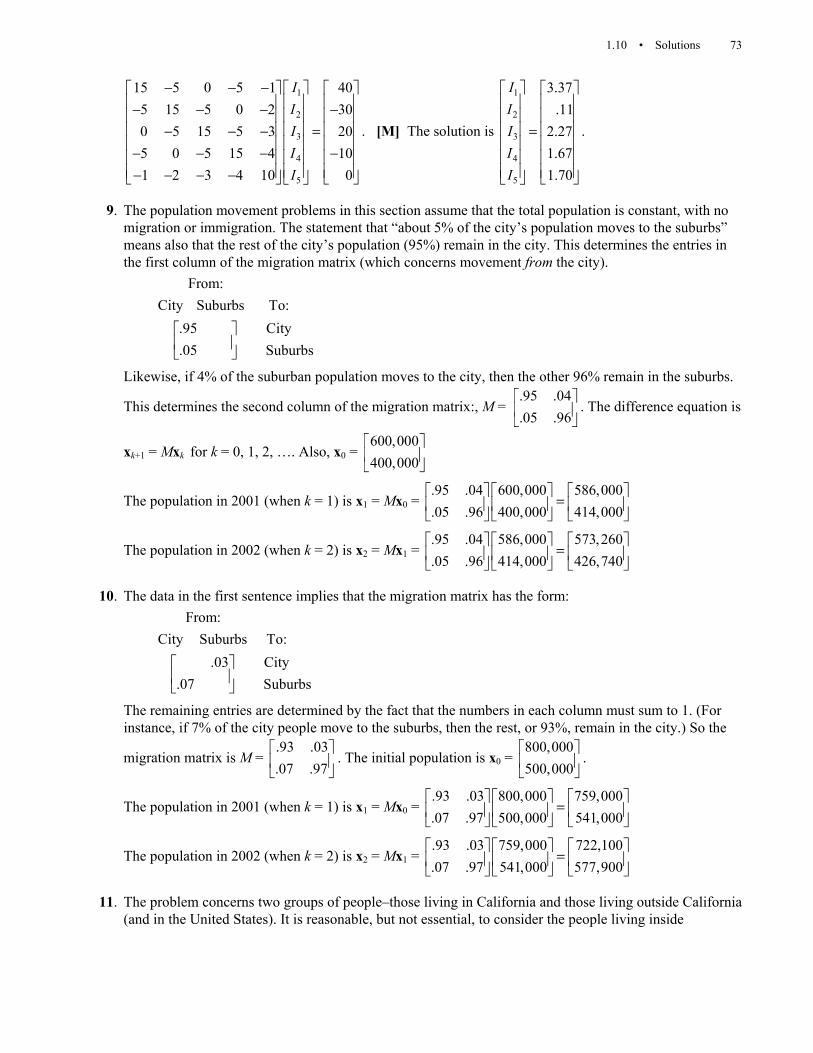
1.10 • Solutions 73
1
2
3
4
5
15 5 0 5 1 405 15 5 0 2 300 5 15 5 3 205 0 5 15 4 101 2 3 4 10 0
IIIII
− − − − − − − =− − − − − − − − − − −
. [M] The solution is
1
2
3
4
5
3.37.11
2.271.671.70
IIIII
=
.
9. The population movement problems in this section assume that the total population is constant, with no migration or immigration. The statement that “about 5% of the city’s population moves to the suburbs” means also that the rest of the city’s population (95%) remain in the city. This determines the entries in the first column of the migration matrix (which concerns movement from the city).
From:
City Suburbs To:.95 City.05 Suburbs
Likewise, if 4% of the suburban population moves to the city, then the other 96% remain in the suburbs.
This determines the second column of the migration matrix:, M = .95 .04.05 .96
. The difference equation is
xk+1 = Mxk for k = 0, 1, 2, …. Also, x0 = 600,000400,000
The population in 2001 (when k = 1) is x1 = Mx0 = .95 .04 600,000 586,000.05 .96 400,000 414,000
=
The population in 2002 (when k = 2) is x2 = Mx1 = .95 .04 586,000 573,260.05 .96 414,000 426,740
=
10. The data in the first sentence implies that the migration matrix has the form:
From:
City Suburbs To:.03 City
.07 Suburbs
The remaining entries are determined by the fact that the numbers in each column must sum to 1. (For instance, if 7% of the city people move to the suburbs, then the rest, or 93%, remain in the city.) So the
migration matrix is M = .93 .03.07 .97
. The initial population is x0 = 800,000500,000
.
The population in 2001 (when k = 1) is x1 = Mx0 = .93 .03 800,000 759,000.07 .97 500,000 541,000
=
The population in 2002 (when k = 2) is x2 = Mx1 = .93 .03 759,000 722,100.07 .97 541,000 577,900
=
11. The problem concerns two groups of people–those living in California and those living outside California (and in the United States). It is reasonable, but not essential, to consider the people living inside
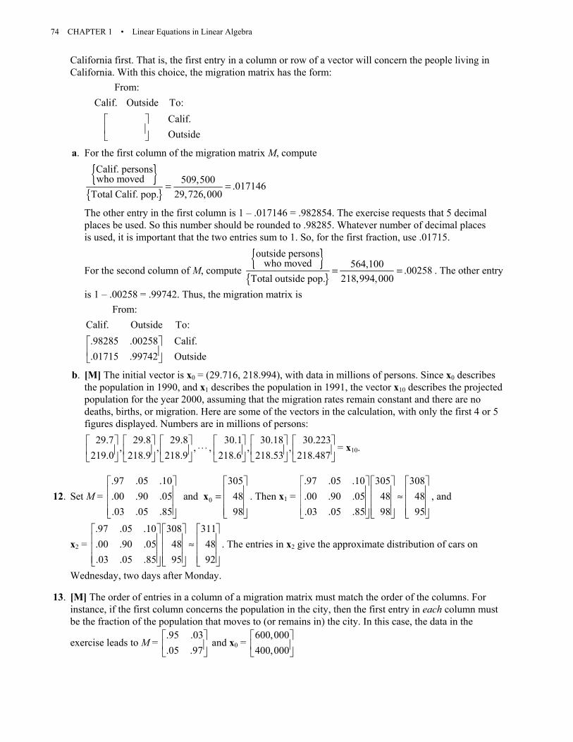
74 CHAPTER 1 • Linear Equations in Linear Algebra
California first. That is, the first entry in a column or row of a vector will concern the people living in California. With this choice, the migration matrix has the form:
From:
Calif. Outside To:Calif.Outside
a. For the first column of the migration matrix M, compute
{ }
{ }
Calif. personswho moved 509,500 .017146
Total Calif. pop. 29,726,000= =
The other entry in the first column is 1 – .017146 = .982854. The exercise requests that 5 decimal places be used. So this number should be rounded to .98285. Whatever number of decimal places is used, it is important that the two entries sum to 1. So, for the first fraction, use .01715.
For the second column of M, compute { }
{ }
outside personswho moved 564,100 .00258
Total outside pop. 218,994,000= = . The other entry
is 1 – .00258 = .99742. Thus, the migration matrix is
From:
Calif. Outside To:.98285 .00258 Calif..01715 .99742 Outside
b. [M] The initial vector is x0 = (29.716, 218.994), with data in millions of persons. Since x0 describes the population in 1990, and x1 describes the population in 1991, the vector x10 describes the projected population for the year 2000, assuming that the migration rates remain constant and there are no deaths, births, or migration. Here are some of the vectors in the calculation, with only the first 4 or 5 figures displayed. Numbers are in millions of persons:
29.7 29.8 29.8 30.1 30.18 30.223
, , , , , ,219.0 218.9 218.9 218.6 218.53 218.487
⋅ ⋅ ⋅
= x10.
12. Set M = 0
.97 .05 .10 305
.00 .90 .05 and 48
.03 .05 .85 98
=
x . Then x1 = .97 .05 .10 305 308.00 .90 .05 48 48.03 .05 .85 98 95
≈
, and
x2 = .97 .05 .10 308 311.00 .90 .05 48 48.03 .05 .85 95 92
≈
. The entries in x2 give the approximate distribution of cars on
Wednesday, two days after Monday.
13. [M] The order of entries in a column of a migration matrix must match the order of the columns. For instance, if the first column concerns the population in the city, then the first entry in each column must be the fraction of the population that moves to (or remains in) the city. In this case, the data in the
exercise leads to M = .95 .03.05 .97
and x0 = 600,000400,000

1.10 • Solutions 75
a. Some of the population vectors are
5 10 15 20523,293 472,737 439,417 417,456
, , ,476,707 527,263 560,583 582,544
= = = =
x x x x
The data here shows that the city population is declining and the suburban population is increasing, but the changes in population each year seem to grow smaller.
b. When x0 = 350,000650,000
, the situation is different. Now
5 10 15 20358,523 364,140 367,843 370,283
, , ,641,477 635,860 632,157 629,717
= = = =
x x x x
The city population is increasing slowly and the suburban population is decreasing. No other conclusions are expected. (This example will be analyzed in greater detail later in the text.)
14. Here are Figs. (a) and (b) for Exercise 13, followed by the figure for Exercise 34 in Section 1.1:
10˚
10˚
40˚
40˚
20˚ 20˚
30˚ 30˚
1 2
4 3
0˚
0˚
0˚
0˚
20˚ 20˚
20˚ 20˚
1 2
4 3
10˚
10˚
40˚
40˚
0˚ 0˚
10˚ 10˚
1 2
4 3
(b) Section 1.1(a)
For Fig. (a), the equations are:
1 2 4
2 1 3
3 4 2
4 1 3
4 0 204 20 04 0 204 0 20
T T TT T TT T TT T T
= + + += + + += + + += + + +
To solve the system, rearrange the equations and row reduce the augmented matrix. Interchanging rows 1 and 4 speeds up the calculations. The first five steps are shown in detail.
4 1 0 1 20 1 0 1 4 20 1 0 1 4 20 1 0 1 4 20
1 4 1 0 20 1 4 1 0 20 0 4 0 4 0 0 1 0 1 0~ ~ ~
0 1 4 1 20 0 1 4 1 20 0 1 4 1 20 0 1 4 1 20
1 0 1 4 20 4 1 0 1 20 0 1 4 15 100 0 1 4 15 100
− − − − − − − −
− − − − − −
− − − − − − − −
− − − − − − − −
1 0 1 4 20 1 0 1 4 20 1 0 0 0 10
0 1 0 1 0 0 1 0 1 0 0 1 0 0 10~ ~ ~
0 0 4 2 20 0 0 4 2 20 0 0 1 0 10
0 0 4 14 100 0 0 0 12 120 0 0 0 1 10
~
− − − −
− −⋅ ⋅ ⋅
− −
−
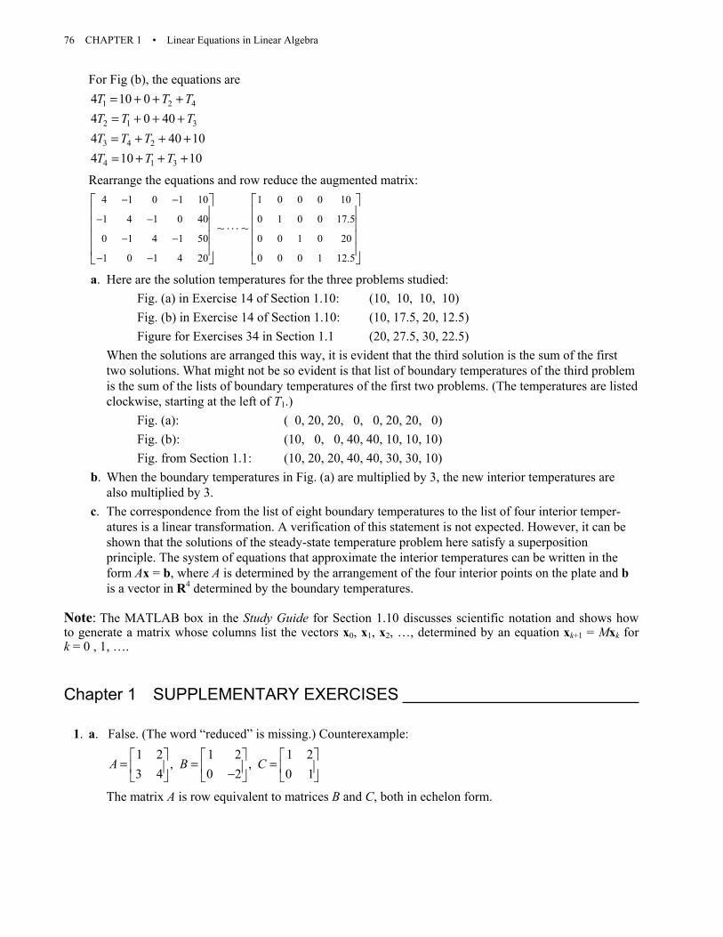
76 CHAPTER 1 • Linear Equations in Linear Algebra
For Fig (b), the equations are
1 2 4
2 1 3
3 4 2
4 1 3
4 10 04 0 404 40 104 10 10
T T TT T TT T TT T T
= + + += + + += + + += + + +
Rearrange the equations and row reduce the augmented matrix:
4 1 0 1 10 1 0 0 0 10
1 4 1 0 40 0 1 0 0 17.5
0 1 4 1 50 0 0 1 0 20
1 0 1 4 20 0 0 0 1 12.5
~ ~
− −
− −
− −
− −
⋅ ⋅ ⋅
a. Here are the solution temperatures for the three problems studied: Fig. (a) in Exercise 14 of Section 1.10: (10, 10, 10, 10) Fig. (b) in Exercise 14 of Section 1.10: (10, 17.5, 20, 12.5) Figure for Exercises 34 in Section 1.1 (20, 27.5, 30, 22.5) When the solutions are arranged this way, it is evident that the third solution is the sum of the first
two solutions. What might not be so evident is that list of boundary temperatures of the third problem is the sum of the lists of boundary temperatures of the first two problems. (The temperatures are listed clockwise, starting at the left of T1.)
Fig. (a): ( 0, 20, 20, 0, 0, 20, 20, 0) Fig. (b): (10, 0, 0, 40, 40, 10, 10, 10) Fig. from Section 1.1: (10, 20, 20, 40, 40, 30, 30, 10) b. When the boundary temperatures in Fig. (a) are multiplied by 3, the new interior temperatures are
also multiplied by 3. c. The correspondence from the list of eight boundary temperatures to the list of four interior temper-
atures is a linear transformation. A verification of this statement is not expected. However, it can be shown that the solutions of the steady-state temperature problem here satisfy a superposition principle. The system of equations that approximate the interior temperatures can be written in the form Ax = b, where A is determined by the arrangement of the four interior points on the plate and b is a vector in R4 determined by the boundary temperatures.
Note: The MATLAB box in the Study Guide for Section 1.10 discusses scientific notation and shows how to generate a matrix whose columns list the vectors x0, x1, x2, …, determined by an equation xk+1 = Mxk for k = 0 , 1, ….
Chapter 1 SUPPLEMENTARY EXERCISES
1. a. False. (The word “reduced” is missing.) Counterexample:
1 2 1 2 1 2
, ,3 4 0 2 0 1
A B C
= = = −
The matrix A is row equivalent to matrices B and C, both in echelon form.

Chapter 1 • Supplementary Exercises 77
b. False. Counterexample: Let A be any n×n matrix with fewer than n pivot columns. Then the equation Ax = 0 has infinitely many solutions. (Theorem 2 in Section 1.2 says that a system has either zero, one, or infinitely many solutions, but it does not say that a system with infinitely many solutions exists. Some counterexample is needed.)
c. True. If a linear system has more than one solution, it is a consistent system and has a free variable. By the Existence and Uniqueness Theorem in Section 1.2, the system has infinitely many solutions.
d. False. Counterexample: The following system has no free variables and no solution:
1 2
2
1 2
152
x xx
x x
+ ==
+ =
e. True. See the box after the definition of elementary row operations, in Section 1.1. If [A b] is transformed into [C d] by elementary row operations, then the two augmented matrices are row equivalent.
f. True. Theorem 6 in Section 1.5 essentially says that when Ax = b is consistent, the solution sets of the nonhomogeneous equation and the homogeneous equation are translates of each other. In this case, the two equations have the same number of solutions.
g. False. For the columns of A to span Rm, the equation Ax = b must be consistent for all b in Rm, not for just one vector b in Rm.
h. False. Any matrix can be transformed by elementary row operations into reduced echelon form, but not every matrix equation Ax = b is consistent.
i. True. If A is row equivalent to B, then A can be transformed by elementary row operations first into B and then further transformed into the reduced echelon form U of B. Since the reduced echelon form of A is unique, it must be U.
j. False. Every equation Ax = 0 has the trivial solution whether or not some variables are free. k. True, by Theorem 4 in Section 1.4. If the equation Ax = b is consistent for every b in Rm, then A must
have a position in every one of its m rows. If A has m pivot positions, then A has m pivot columns, each containing one pivot position.
l. False. The word “unique” should be deleted. Let A be any matrix with m pivot columns but more than m columns altogether. Then the equation Ax = b is consistent and has m basic variables and at least one free variable. Thus the equation does not does not have a unique solution.
m. True. If A has n pivot positions, it has a pivot in each of its n columns and in each of its n rows. The reduced echelon form has a 1 in each pivot position, so the reduced echelon form is the n×n identity matrix.
n. True. Both matrices A and B can be row reduced to the 3×3 identity matrix, as discussed in the previous question. Since the row operations that transform B into I3 are reversible, A can be transformed first into I3 and then into B.
o. True. The reason is essentially the same as that given for question f. p. True. If the columns of A span Rm, then the reduced echelon form of A is a matrix U with a pivot in
each row, by Theorem 4 in Section 1.4. Since B is row equivalent to A, B can be transformed by row operations first into A and then further transformed into U. Since U has a pivot in each row, so does B. By Theorem 4, the columns of B span Rm.
q. False. See Example 5 in Section 1.6. r. True. Any set of three vectors in R2 would have to be linearly dependent, by Theorem 8 in
Section 1.6.

78 CHAPTER 1 • Linear Equations in Linear Algebra
s. False. If a set {v1, v2, v3, v4} were to span R5, then the matrix A = [v1 v2 v3 v4] would have a pivot position in each of its five rows, which is impossible since A has only four columns.
t. True. The vector –u is a linear combination of u and v, namely, –u = (–1)u + 0v. u. False. If u and v are multiples, then Span{u, v} is a line, and w need not be on that line. v. False. Let u and v be any linearly independent pair of vectors and let w = 2v. Then w = 0u + 2v, so w
is a linear combination of u and v. However, u cannot be a linear combination of v and w because if it were, u would be a multiple of v. That is not possible since {u, v} is linearly independent.
w. False. The statement would be true if the condition v1 is not zero were present. See Theorem 7 in Section 1.7. However, if v1 = 0, then {v1, v2, v3} is linearly dependent, no matter what else might be true about v2 and v3.
x. True. “Function” is another word used for “transformation” (as mentioned in the definition of “transformation” in Section 1.8), and a linear transformation is a special type of transformation.
y. True. For the transformation x Ax to map R5 onto R6, the matrix A would have to have a pivot in every row and hence have six pivot columns. This is impossible because A has only five columns.
z. False. For the transformation x Ax to be one-to-one, A must have a pivot in each column. Since A has n columns and m pivots, m might be less than n.
2. If a ≠ 0, then x = b/a; the solution is unique. If a = 0, and b ≠ 0, the solution set is empty, because 0x = 0 ≠ b. If a = 0 and b = 0, the equation 0x = 0 has infinitely many solutions.
3. a. Any consistent linear system whose echelon form is
* * * * * * 0 * *
0 * * or 0 0 * or 0 0 *0 0 0 0 0 0 0 0 0 0 0 0
b. Any consistent linear system whose coefficient matrix has reduced echelon form I3. c. Any inconsistent linear system of three equations in three variables.
4. Since there are three pivots (one in each row), the augmented matrix must reduce to the form
* * *
0 * *0 0 *
. A solution of Ax = b exists for all b because there is a pivot in each row of A. Each
solution is unique because there are no free variables.
5. a. 1 3 1 3
~4 8 0 12 8 4
k kh h k
− −
. If h = 12 and k ≠ 2, the second row of the augmented matrix
indicates an inconsistent system of the form 0x2 = b, with b nonzero. If h = 12, and k = 2, there is only one nonzero equation, and the system has infinitely many solutions. Finally, if h ≠ 12, the coefficient matrix has two pivots and the system has a unique solution.
b. 2 1 2 1
~6 2 0 3 1
h hk k h
− − − +
. If k + 3h = 0, the system is inconsistent. Otherwise, the
coefficient matrix has two pivots and the system has a unique solution.

Chapter 1 • Supplementary Exercises 79
6. a. Set 1 2 34 2 7
, ,8 3 10
− = = = −
v v v , and 53
− = −
b . “Determine if b is a linear combination of v1, v2,
v3.” Or, “Determine if b is in Span{v1, v2, v3}.” To do this, compute 4 2 7 5 4 2 7 5
~8 3 10 3 0 1 4 7
− − − − − − −
. The system is consistent, so b is in Span{v1, v2, v3}.
b. Set A = 4 2 7 5
,8 3 10 3
− − = − −
b . “Determine if b is a linear combination of the columns of A.”
c. Define T(x) = Ax. “Determine if b is in the range of T.”
7. a. Set 1 2 3
2 4 25 , 1 , 17 5 3
− − = − = = − −
v v v and 1
2
3
bbb
=
b . “Determine if v1, v2, v3 span R3.” To do this, row
reduce [v1 v2 v3]:
2 4 2 2 4 2 2 4 25 1 1 ~ 0 9 4 ~ 0 9 47 5 3 0 9 4 0 0 0
− − − − − − − − − − − − −
. The matrix does not have a pivot in each row, so
its columns do not span R3, by Theorem 4 in Section 1.4.
b. Set A = 2 4 25 1 17 5 3
− − − − −
. “Determine if the columns of A span R3.”
c. Define T(x) = Ax. “Determine if T maps R3 onto R3.”
8. a. * * * * 0 *
, ,0 * 0 0 0 0
b. * *
0 *0 0
9. The first line is the line spanned by 12
. The second line is spanned by 21
. So the problem is to write
56
as the sum of a multiple of 12
and a multiple of 21
. That is, find x1 and x2 such that
1 22 1 51 2 6
x x
+ =
. Reduce the augmented matrix for this equation:
2 1 5 1 2 6 1 2 6 1 2 6 1 0 4 / 3
~ ~ ~ ~1 2 6 2 1 5 0 3 7 0 1 7 / 3 0 1 7 / 3 − −
Thus, 4 73 3
5 2 16 1 2
= +
or 5 8/ 3 7 / 36 4 / 3 14 / 3
= +
.
10. The line through a1 and the origin and the line through a2 and the origin determine a “grid” on the x1x2-plane as shown below. Every point in R2 can be described uniquely in terms of this grid. Thus, b can

80 CHAPTER 1 • Linear Equations in Linear Algebra
be reached from the origin by traveling a certain number of units in the a1-direction and a certain number of units in the a2-direction.
x1
x2
a2
a1
b
11. A solution set is a line when the system has one free variable. If the coefficient matrix is 2×3, then two of
the columns should be pivot columns. For instance, take 1 2 *0 3 *
. Put anything in column 3. The
resulting matrix will be in echelon form. Make one row replacement operation on the second row to
create a matrix not in echelon form, such as 1 2 1 1 2 1
~0 3 1 1 5 2
12. A solution set is a plane where there are two free variables. If the coefficient matrix is 2×3, then only one column can be a pivot column. The echelon form will have all zeros in the second row. Use a row
replacement to create a matrix not in echelon form. For instance, let A =1 2 31 2 3
.
13. The reduced echelon form of A looks like 1 0 *0 1 *0 0 0
E =
. Since E is row equivalent to A, the equation
Ex = 0 has the same solutions as Ax = 0. Thus 1 0 * 3 00 1 * 2 00 0 0 1 0
− =
.
By inspection, 1 0 30 1 20 0 0
E−
=
.
14. Row reduce the augmented matrix for 1 21 0
2 0a
x xa a
+ = + (*).
2
1 01 0 1 0~
2 0 0 (2 )(1 ) 00 2 0
aa aa a a aa a
= + − ++ −
The equation (*) has a nontrivial solution only when (2 – a)(1 + a) = 0. So the vectors are linearly independent for all a except a = 2 and a = –1.
15. a. If the three vectors are linearly independent, then a, c, and f must all be nonzero. (The converse is true, too.) Let A be the matrix whose columns are the three linearly independent vectors. Then

Chapter 1 • Supplementary Exercises 81
A must have three pivot columns. (See Exercise 30 in Section 1.7, or realize that the equation Ax = 0 has only the trivial solution and so there can be no free variables in the system of equations.) Since A is 3×3, the pivot positions are exactly where a, c, and f are located.
b. The numbers a, …, f can have any values. Here's why. Denote the columns by v1, v2, and v3. Observe that v1 is not the zero vector. Next, v2 is not a multiple of v1 because the third entry of v2 is nonzero. Finally, v3 is not a linear combination of v1 and v2 because the fourth entry of v3 is nonzero. By Theorem 7 in Section 1.7, {v1, v2, v3} is linearly independent.
16. Denote the columns from right to left by v1, …, v4. The “first” vector v1 is nonzero, v2 is not a multiple of v1 (because the third entry of v2 is nonzero), and v3 is not a linear combination of v1 and v2 (because the second entry of v3 is nonzero). Finally, by looking at first entries in the vectors, v4 cannot be a linear combination of v1, v2, and v3. By Theorem 7 in Section 1.7, the columns are linearly independent.
17. Here are two arguments. The first is a “direct” proof. The second is called a “proof by contradiction.” i. Since {v1, v2, v3} is a linearly independent set, v1 ≠ 0. Also, Theorem 7 shows that v2 cannot be a
multiple of v1, and v3 cannot be a linear combination of v1 and v2. By hypothesis, v4 is not a linear combination of v1, v2, and v3. Thus, by Theorem 7, {v1, v2, v3, v4} cannot be a linearly dependent set and so must be linearly independent.
ii. Suppose that {v1, v2, v3, v4} is linearly dependent. Then by Theorem 7, one of the vectors in the set is a linear combination of the preceding vectors. This vector cannot be v4 because v4 is not in Span{v1, v2, v3}. Also, none of the vectors in {v1, v2, v3} is a linear combinations of the preceding vectors, by Theorem 7. So the linear dependence of {v1, v2, v3, v4} is impossible. Thus {v1, v2, v3, v4} is linearly independent.
18. Suppose that c1 and c2 are constants such that c1v1 + c2(v1 + v2) = 0 (*) Then (c1 + c2)v1 + c2v2 = 0. Since v1 and v2 are linearly independent, both c1 + c2 = 0 and c2 = 0. It
follows that both c1 and c2 in (*) must be zero, which shows that {v1, v1 + v2} is linearly independent.
19. Let M be the line through the origin that is parallel to the line through v1, v2, and v3. Then v2 – v1 and v3 – v1 are both on M. So one of these two vectors is a multiple of the other, say v2 – v1 = k(v3 – v1). This equation produces a linear dependence relation (k – 1)v1 + v2 – kv3 = 0.
A second solution: A parametric equation of the line is x = v1 + t(v2 – v1). Since v3 is on the line, there is some t0 such that v3 = v1 + t0(v2 – v1) = (1 – t0)v1 + t0v2. So v3 is a linear combination of v1 and v2, and {v1, v2, v3} is linearly dependent.
20. If T(u) = v, then since T is linear, T(–u) = T((–1)u) = (–1)T(u) = –v.
21. Either compute T(e1), T(e2), and T(e3) to make the columns of A, or write the vectors vertically in the definition of T and fill in the entries of A by inspection:
1 1
2 2
3 3
? ? ? 1 0 0? ? , 0 1 0? ? ? 0 0 1
x xA A x x A
x x
= = − = −
x
22. By Theorem 12 in Section 1.9, the columns of A span R3. By Theorem 4 in Section 1.4, A has a pivot in each of its three rows. Since A has three columns, each column must be a pivot column. So the equation

82 CHAPTER 1 • Linear Equations in Linear Algebra
Ax = 0 has no free variables, and the columns of A are linearly independent. By Theorem 12 in Section 1.9, the transformation x Ax is one-to-one.
23. 4 5 4 3 5
implies that 3 0 3 4 0
a b a bb a a b
=− − =
+ = . Solve:
4 3 5 4 3 5 4 3 5 4 0 16 / 5 1 0 4 / 5
~ ~ ~ ~3 4 0 0 25/ 4 15/ 4 0 1 3/ 5 0 1 3/ 5 0 1 3/ 5
− − − − − − −
Thus a = 4/5 and b = –3/5.
24. The matrix equation displayed gives the information 2 4 2 5a b− = and 4 2 0.a b+ = Solve for a and b: 2 4 2 5 1 2 5 1 0 1/ 52 4 2 5 ~ ~ ~
4 2 0 0 10 4 5 0 1 2 / 5 0 1 2 / 5
− −−
− − −
So 1/ 5, 2 / 5.a b= = −
25. a. The vector lists the number of three-, two-, and one-bedroom apartments provided when x1 floors of plan A are constructed.
b. 1 2 3
3 4 57 4 38 8 9
x x x + +
c. [M] Solve 1 2 3
3 4 5 667 4 3 748 8 9 136
x x x + + =
1 3
2 3
3 4 5 66 1 0 1/ 2 2 (1/ 2) 27 4 3 74 ~ 0 1 13/8 15 (13/8) 158 8 9 136 0 0 0 0 0 0
x xx x
− − = ⋅ ⋅ ⋅ + = =
The general solution is
1 3
2 3 3
3 3
2 (1/ 2) 2 1/ 215 (13/8) 15 13/8
0 1
x xx x xx x
+ = = − = + −
x
However, the only feasible solutions must have whole numbers of floors for each plan. Thus, x3 must be a multiple of 8, to avoid fractions. One solution, for x3 = 0, is to use 2 floors of plan A and 15 floors of plan B. Another solution, for x3 = 8, is to use 6 floors of plan A , 2 floors of plan B, and 8 floors of plan C. These are the only feasible solutions. A larger positive multiple of 8 for x3 makes x2 negative. A negative value for x3, of course, is not feasible either.

83
2.1 SOLUTIONS
Notes: The definition here of a matrix product AB gives the proper view of AB for nearly all matrix calculations. (The dual fact about the rows of A and the rows of AB is seldom needed, mainly because vectors here are usually written as columns.) I assign Exercise 13 and most of Exercises 17–22 to reinforce the definition of AB.
Exercises 23 and 24 are used in the proof of the Invertible Matrix Theorem, in Section 2.3. Exercises 23–25 are mentioned in a footnote in Section 2.2. A class discussion of the solutions of Exercises 23–25 can provide a transition to Section 2.2. Or, these exercises could be assigned after starting Section 2.2.
Exercises 27 and 28 are optional, but they are mentioned in Example 4 of Section 2.4. Outer products also appear in Exercises 31–34 of Section 4.6 and in the spectral decomposition of a symmetric matrix, in Section 7.1. Exercises 29–33 provide good training for mathematics majors.
1. 2 0 1 4 0 2
2 ( 2)4 5 2 8 10 4
A− −
− = − = − − − . Next, use B – 2A = B + (–2A):
7 5 1 4 0 2 3 5 3
21 4 3 8 10 4 7 6 7
B A− − −
− = + = − − − − − −
The product AC is not defined because the number of columns of A does not match the number of rows
of C. 1 2 3 5 1 3 2( 1) 1 5 2 4 1 132 1 1 4 2 3 1( 1) 2 5 1 4 7 6
CD⋅ + − ⋅ + ⋅
= = = − − − ⋅ + − − ⋅ + ⋅ − − . For mental computation, the
row-column rule is probably easier to use than the definition.
2. 2 0 1 7 5 1 2 14 0 10 1 2 16 10 1
2 24 5 2 1 4 3 4 2 5 8 2 6 6 13 4
A B− − + − − + −
+ = + = = − − − + − − − − −
The expression 3C – E is not defined because 3C has 2 columns and –E has only 1 column.
1 2 7 5 1 1 7 2 1 1( 5) 2( 4) 1 1 2( 3) 9 13 52 1 1 4 3 2 7 1 1 2( 5) 1( 4) 2 1 1( 3) 13 6 5
CB− ⋅ + ⋅ − + − ⋅ + − − −
= = = − − − − ⋅ + ⋅ − − + − − ⋅ + − − −
The product EB is not defined because the number of columns of E does not match the number of rows of R.

84 CHAPTER 2 • Matrix Algebra
3. 23 0 4 1 3 4 0 ( 1) 1 1
30 3 5 2 0 5 3 ( 2) 5 5
I A− − − − −
− = − = = − − − − −
2 24 1 12 3
(3 ) 3( ) 35 2 15 6
I A I A− −
= = = − − , or
23 0 4 1 3 4 0 3( 1) 0 12 3
(3 )0 3 5 2 0 3 5 0 3( 2) 15 6
I A− ⋅ + − + −
= = = − + ⋅ + − −
4. 3
9 1 3 5 0 0 4 1 35 8 7 6 0 5 0 8 2 6
4 1 8 0 0 5 4 1 3A I
− − − = − − − = − − − −
3 3
9 1 3 45 5 15(5 ) 5( ) 5 5 8 7 6 40 35 30
4 1 8 20 5 40I A I A A
− − = = = − − = − − − −
, or
3
5 0 0 9 1 3(5 ) 0 5 0 8 7 6
0 0 5 4 1 8I A
− = − − −
5 9 0 0 5( 1) 0 0 5 3 0 0 45 5 15
0 5( 8) 0 0 5 7 0 0 5( 6) 0 45 35 300 0 5( 4) 0 0 5 1 0 0 5 8 20 5 40
⋅ + + − + + ⋅ + + − = + − + + ⋅ + + − + = − − + + − + + ⋅ + + ⋅ −
5. a. 1 2
1 2 7 1 2 43 2
5 4 7 , 5 4 62 1
2 3 12 2 3 7A A
− − − − = = = = − − − − −
b b
[ ]1 2
7 47 6
12 7AB A A
− = = − −
b b
b. 1 2 1 3 2( 2) 1( 2) 2 1 7 4
3 25 4 5 3 4( 2) 5( 2) 4 1 7 6
2 12 3 2 3 3( 2) 2( 2) 3 1 12 7
− − ⋅ + − − − + ⋅ − − = ⋅ + − − + ⋅ = − − − ⋅ − − − − ⋅ −
6. a. 1 2
4 2 0 4 2 141 3
3 0 3 , 3 0 92 1
3 5 13 3 5 4A A
− − = − = − = − = − −
b b
[ ]1 2
0 143 9
13 4AB A A
= = − −
b b
b. 4 2 4 1 2 2 4 3 2( 1) 0 14
1 33 0 3 1 0 2 3 3 0( 1) 3 9
2 13 5 3 1 5 2 3 3 5( 1) 13 4
− ⋅ − ⋅ ⋅ − − − = − ⋅ + ⋅ − ⋅ + − = − − − ⋅ + ⋅ ⋅ + −

2.1 • Solutions 85
7. Since A has 3 columns, B must match with 3 rows. Otherwise, AB is undefined. Since AB has 7 columns, so does B. Thus, B is 3×7.
8. The number of rows of B matches the number of rows of BC, so B has 3 rows.
9. 2 5 4 5 23 10 5
,3 1 3 9 15
kAB
k k− − +
= = − − + while
4 5 2 5 23 153 3 1 6 3 15
BAk k k
− = = − − +
.
Then AB = BA if and only if –10 + 5k = 15 and –9 = 6 – 3k, which happens if and only if k = 5.
10. 2 3 8 4 1 7 2 3 5 2 1 7
,4 6 5 5 2 14 4 6 3 1 2 14
AB AC− − − − −
= = = = − − − −
11. 1 1 1 2 0 0 2 3 51 2 3 0 3 0 2 6 151 4 5 0 0 5 2 12 25
AD = =
2 0 0 1 1 1 2 2 20 3 0 1 2 3 3 6 90 0 5 1 4 5 5 20 25
DA = =
Right-multiplication (that is, multiplication on the right) by the diagonal matrix D multiplies each column of A by the corresponding diagonal entry of D. Left-multiplication by D multiplies each row of A by the corresponding diagonal entry of D. To make AB = BA, one can take B to be a multiple of I3. For instance, if B = 4I3, then AB and BA are both the same as 4A.
12. Consider B = [b1 b2]. To make AB = 0, one needs Ab1 = 0 and Ab2 = 0. By inspection of A, a suitable
b1 is 2
,1
or any multiple of 21
. Example: 2 6
.1 3
B
=
13. Use the definition of AB written in reverse order: [Ab1 ⋅ ⋅ ⋅ Abp] = A[b1 ⋅ ⋅ ⋅ bp]. Thus [Qr1 ⋅ ⋅ ⋅ Qrp] = QR, when R = [r1 ⋅ ⋅ ⋅ rp].
14. By definition, UQ = U[q1 ⋅ ⋅ ⋅ q4] = [Uq1 ⋅ ⋅ ⋅ Uq4]. From Example 6 of Section 1.8, the vector Uq1 lists the total costs (material, labor, and overhead) corresponding to the amounts of products B and C specified in the vector q1. That is, the first column of UQ lists the total costs for materials, labor, and overhead used to manufacture products B and C during the first quarter of the year. Columns 2, 3, and 4 of UQ list the total amounts spent to manufacture B and C during the 2nd, 3rd, and 4th quarters, respectively.
15. a. False. See the definition of AB. b. False. The roles of A and B should be reversed in the second half of the statement. See the box after
Example 3. c. True. See Theorem 2(b), read right to left. d. True. See Theorem 3(b), read right to left. e. False. The phrase “in the same order” should be “in the reverse order.” See the box after Theorem 3.
16. a. False. AB must be a 3×3 matrix, but the formula for AB implies that it is 3×1. The plus signs should be just spaces (between columns). This is a common mistake.
b. True. See the box after Example 6. c. False. The left-to-right order of B and C cannot be changed, in general.

86 CHAPTER 2 • Matrix Algebra
d. False. See Theorem 3(d). e. True. This general statement follows from Theorem 3(b).
17. Since [ ]1 2 31 2 1
,6 9 3
AB A A A− −
= = − b b b the first column of B satisfies the equation
1.
6A
− =
x Row reduction:[ ]11 2 1 1 0 7
~ ~2 5 6 0 1 4
A A− −
− b . So b1 =
7.
4
Similarly,
[ ]21 2 2 1 0 8
~ ~2 5 9 0 1 5
A A− −
− − − b and b2 =
8.
5− −
Note: An alternative solution of Exercise 17 is to row reduce [A Ab1 Ab2] with one sequence of row operations. This observation can prepare the way for the inversion algorithm in Section 2.2.
18. The first two columns of AB are Ab1 and Ab2. They are equal since b1 and b2 are equal.
19. (A solution is in the text). Write B = [b1 b2 b3]. By definition, the third column of AB is Ab3. By hypothesis, b3 = b1 + b2. So Ab3 = A(b1 + b2) = Ab1 + Ab2, by a property of matrix-vector multiplication. Thus, the third column of AB is the sum of the first two columns of AB.
20. The second column of AB is also all zeros because Ab2 = A0 = 0.
21. Let bp be the last column of B. By hypothesis, the last column of AB is zero. Thus, Abp = 0. However, bp is not the zero vector, because B has no column of zeros. Thus, the equation Abp = 0 is a linear dependence relation among the columns of A, and so the columns of A are linearly dependent.
Note: The text answer for Exercise 21 is, “The columns of A are linearly dependent. Why?” The Study Guide supplies the argument above, in case a student needs help.
22. If the columns of B are linearly dependent, then there exists a nonzero vector x such that Bx = 0. From this, A(Bx) = A0 and (AB)x = 0 (by associativity). Since x is nonzero, the columns of AB must be linearly dependent.
23. If x satisfies Ax = 0, then CAx = C0 = 0 and so Inx = 0 and x = 0. This shows that the equation Ax = 0 has no free variables. So every variable is a basic variable and every column of A is a pivot column. (A variation of this argument could be made using linear independence and Exercise 30 in Section 1.7.) Since each pivot is in a different row, A must have at least as many rows as columns.
24. Take any b in Rm. By hypothesis, ADb = Imb = b. Rewrite this equation as A(Db) = b. Thus, the vector x = Db satisfies Ax = b. This proves that the equation Ax = b has a solution for each b in Rm. By Theorem 4 in Section 1.4, A has a pivot position in each row. Since each pivot is in a different column, A must have at least as many columns as rows.
25. By Exercise 23, the equation CA = In implies that (number of rows in A) > (number of columns), that is, m > n. By Exercise 24, the equation AD = Im implies that (number of rows in A) < (number of columns), that is, m < n. Thus m = n. To prove the second statement, observe that DAC = (DA)C = InC = C, and also DAC = D(AC) = DIm = D. Thus C = D. A shorter calculation is
C = InC = (DA)C = D(AC) = DIn = D
26. Write I3 =[e1 e2 e3] and D = [d1 d2 d3]. By definition of AD, the equation AD = I3 is equivalent |to the three equations Ad1 = e1, Ad2 = e2, and Ad3 = e3. Each of these equations has at least one solution because the columns of A span R3. (See Theorem 4 in Section 1.4.) Select one solution of each equation and use them for the columns of D. Then AD = I3.

2.1 • Solutions 87
27. The product uTv is a 1×1 matrix, which usually is identified with a real number and is written without the matrix brackets.
[ ]2 3 4 2 3 4Tab a b cc
= − − = − + −
u v , [ ]23 2 3 44
T a b c a b c− = = − + − −
v u
[ ]2 2 2 23 3 3 34 4 4 4
Ta b c
a b c a b ca b c
− − − − = = − − − −
uv
[ ]2 3 4
2 3 4 2 3 42 3 4
Ta a a ab b b bc c c c
− − = − − = − − − −
vu
28. Since the inner product uTv is a real number, it equals its transpose. That is, uTv = (uTv)T = vT (uT)T = vTu, by Theorem 3(d) regarding the transpose of a product of matrices and by
Theorem 3(a). The outer product uvT is an n×n matrix. By Theorem 3, (uvT)T = (vT)TuT = vuT.
29. The (i, j)-entry of A(B + C) equals the (i, j)-entry of AB + AC, because
1 1 1
( )n n n
ik kj kj ik kj ik kjk k k
a b c a b a c= = =
+ = +∑ ∑ ∑
The (i, j)-entry of (B + C)A equals the (i, j)-entry of BA + CA, because
1 1 1( )
n n n
ik ik kj ik kj ik kjk k k
b c a b a c a= = =
+ = +∑ ∑ ∑
30. The (i, j))-entries of r(AB), (rA)B, and A(rB) are all equal, because
1 1 1
( ) ( )n n n
ik kj ik kj ik kjk k k
r a b ra b a rb= = =
= =∑ ∑ ∑
31. Use the definition of the product ImA and the fact that Imx = x for x in Rm. ImA = Im[a1 ⋅ ⋅ ⋅ an] = [Ima1 ⋅ ⋅ ⋅ Iman] = [a1 ⋅ ⋅ ⋅ an] = A
32. Let ej and aj denote the jth columns of In and A, respectively. By definition, the jth column of AIn is Aej, which is simply aj because ej has 1 in the jth position and zeros elsewhere. Thus corresponding columns of AIn and A are equal. Hence AIn = A.
33. The (i, j)-entry of (AB)T is the ( j, i)-entry of AB, which is 1 1j i jn nia b a b+ ⋅⋅⋅ +
The entries in row i of BT are b1i, … , bni, because they come from column i of B. Likewise, the entries in column j of AT are aj1, …, ajn, because they come from row j of A. Thus the (i, j)-entry in BTAT is
1 1j i jn nia b a b+ + , as above.
34. Use Theorem 3(d), treating x as an n×1 matrix: (ABx)T = xT(AB)T = xTBTAT.
35. [M] The answer here depends on the choice of matrix program. For MATLAB, use the help command to read about zeros, ones, eye, and diag. For other programs see the appendices in the Study Guide. (The TI calculators have fewer single commands that produce special matrices.)

88 CHAPTER 2 • Matrix Algebra
36. [M] The answer depends on the choice of matrix program. In MATLAB, the command rand(6,4) creates a 6×4 matrix with random entries uniformly distributed between 0 and 1. The command
round(19*(rand(6,4)–.5))
creates a random 6×4 matrix with integer entries between –9 and 9. The same result is produced by the command randomint in the Laydata Toolbox on text website. For other matrix programs see the appendices in the Study Guide.
37. [M] (A + I)(A – I) – (A2 – I) = 0 for all 4×4 matrices. However, (A + B)(A – B) – A2 – B2 is the zero matrix only in the special cases when AB = BA. In general,
(A + B)(A – B) = A(A – B) + B(A – B) = AA – AB + BA – BB.
38. [M] The equality (AB)T = ATBT is very likely to be false for 4×4 matrices selected at random.
39. [M] The matrix S “shifts” the entries in a vector (a, b, c, d, e) to yield (b, c, d, e, 0). The entries in S2 result from applying S to the columns of S, and similarly for S3 , and so on. This explains the patterns of entries in the powers of S:
2 3 4
0 0 1 0 0 0 0 0 1 0 0 0 0 0 10 0 0 1 0 0 0 0 0 1 0 0 0 0 0
, ,0 0 0 0 1 0 0 0 0 0 0 0 0 0 00 0 0 0 0 0 0 0 0 0 0 0 0 0 00 0 0 0 0 0 0 0 0 0 0 0 0 0 0
S S S
= = =
S5 is the 5×5 zero matrix. S6 is also the 5×5 zero matrix.
40. [M] 5 10.3318 .3346 .3336 .333337 .333330 .333333.3346 .3323 .3331 , .333330 .333336 .333334.3336 .3331 .3333 .333333 .333334 .333333
A A = =
The entries in A20 all agree with .3333333333 to 9 or 10 decimal places. The entries in A30 all agree with .33333333333333 to at least 14 decimal places. The matrices appear to approach the matrix
1/ 3 1/ 3 1/ 31/ 3 1/ 3 1/ 31/ 3 1/ 3 1/ 3
. Further exploration of this behavior appears in Sections 4.9 and 5.2.
Note: The MATLAB box in the Study Guide introduces basic matrix notation and operations, including the commands that create special matrices needed in Exercises 35, 36 and elsewhere. The Study Guide appendices treat the corresponding information for the other matrix programs.
2.2 SOLUTIONS
Notes: The text includes the matrix inversion algorithm at the end of the section because this topic is popular. Students like it because it is a simple mechanical procedure. However, I no longer cover it in my classes because technology is readily available to invert a matrix whenever needed, and class time is better spent on more useful topics such as partitioned matrices. The final subsection is independent of the inversion algorithm and is needed for Exercises 35 and 36.
Key Exercises: 8, 11–24, 35. (Actually, Exercise 8 is only helpful for some exercises in this section. Section 2.3 has a stronger result.) Exercises 23 and 24 are used in the proof of the Invertible Matrix Theorem (IMT) in Section 2.3, along with Exercises 23 and 24 in Section 2.1. I recommend letting students work on two or more of these four exercises before proceeding to Section 2.3. In this way students participate in the

2.2 • Solutions 89
proof of the IMT rather than simply watch an instructor carry out the proof. Also, this activity will help students understand why the theorem is true.
1. 18 6 4 6 2 31
5 4 5 8 5/ 2 432 30
− − − = = − −−
2. 13 2 4 2 2 11
7 4 7 3 7 / 2 3/ 212 14
− − − = = − −−
3. 18 5 5 5 5 5 1 11 1 or
7 5 7 8 7 8 1.4 1.640 ( 35) 5
− − − − − = = − − − − −− − −
4. ( )13 4 8 4 8 4 2 11 1 or
7 8 7 3 7 3 7 / 4 3/ 424 28 4
−− − − − = = − − − −− − −
5. The system is equivalent to Ax = b, where8 6 2
and =5 4 1
A
= − b , and the solution is
x = A–1b = 2 3 2 7
.5/ 2 4 1 9
− = − − −
Thus x1 = 7 and x2 = –9.
6. The system is equivalent to Ax = b, where8 5 9
and 7 5 11
A
= = − − b , and the solution is x = A–1b. To
compute this by hand, the arithmetic is simplified by keeping the fraction 1/det(A) in front of the matrix for A–1. (The Study Guide comments on this in its discussion of Exercise 7.) From Exercise 3,
x = A–1b = 5 5 9 10 21 17 8 11 25 55 5
− − − − − = − = −
. Thus x1 = 2 and x2 = –5.
7. a. 11 2 12 2 12 2 6 11 1 or
5 12 5 1 5 1 2.5 .51 12 2 5 2
− − − − = = − − −⋅ − ⋅
x = A–1b1 = 12 2 1 18 91 1
5 1 3 8 42 2− − − −
= = − . Similar calculations give
1 1 12 3 4
11 6 13, ,
5 2 5A A A− − −
= = = − − − b b b .
b. [A b1 b2 b3 b4] = 1 2 1 1 2 35 12 3 5 6 5
− −
1 2 1 1 2 3 1 2 1 1 2 3
~ ~0 2 8 10 4 10 0 1 4 5 2 5
− − − − − − − −
1 0 9 11 6 13
~0 1 4 5 2 5
− − − −
The solutions are 9 11 6 13
, , , and ,4 5 2 5
− − − −
the same as in part (a).

90 CHAPTER 2 • Matrix Algebra
Note: The Study Guide also discusses the number of arithmetic calculations for this Exercise 7, stating that when A is large, the method used in (b) is much faster than using A–1.
8. Left-multiply each side of the equation AD = I by A–1 to obtain A–1AD = A–1I, ID = A–1, and D = A–1. Parentheses are routinely suppressed because of the associative property of matrix multiplication.
9. a. True, by definition of invertible. b. False. See Theorem 6(b).
c. False. If 1 10 0
A
=
, then ab – cd = 1 – 0 ≠ 0, but Theorem 4 shows that this matrix is not invertible,
because ad – bc = 0. d. True. This follows from Theorem 5, which also says that the solution of Ax = b is unique, for each b. e. True, by the box just before Example 6.
10. a. False. The product matrix is invertible, but the product of inverses should be in the reverse order. See Theorem 6(b). b. True, by Theorem 6(a). c. True, by Theorem 4. d. True, by Theorem 7. e. False. The last part of Theorem 7 is misstated here.
11. (The proof can be modeled after the proof of Theorem 5.) The n×p matrix B is given (but is arbitrary). Since A is invertible, the matrix A–1B satisfies AX = B, because A(A–1B) = A A–1B = IB = B. To show this solution is unique, let X be any solution of AX = B. Then, left-multiplication of each side by A–1 shows that X must be A–1B:
A–1 (AX) = A–1B, IX = A–1B, and X = A–1B.
12. If you assign this exercise, consider giving the following Hint: Use elementary matrices and imitate the proof of Theorem 7. The solution in the Instructor’s Edition follows this hint. Here is another solution, based on the idea at the end of Section 2.2.
Write B = [b1 ⋅ ⋅ ⋅ bp] and X = [u1 ⋅ ⋅ ⋅ up]. By definition of matrix multiplication, AX = [Au1 ⋅ ⋅ ⋅ Aup]. Thus, the equation AX = B is equivalent to the p systems:
Au1 = b1, … Aup = bp Since A is the coefficient matrix in each system, these systems may be solved simultaneously, placing the
augmented columns of these systems next to A to form [A b1 ⋅ ⋅ ⋅ bp] = [A B]. Since A is invertible, the solutions u1, …, up are uniquely determined, and [A b1 ⋅ ⋅ ⋅ bp] must row reduce to [I u1 ⋅ ⋅ ⋅ up] = [I X]. By Exercise 11, X is the unique solution A–1B of AX = B.
13. Left-multiply each side of the equation AB = AC by A–1 to obtain A–1AB = A–1AC, IB = IC, and B = C. This conclusion does not always follow when A is singular. Exercise 10 of Section 2.1 provides a
counterexample.
14. Right-multiply each side of the equation (B – C)D = 0 by D–1 to obtain (B – C)DD–1 = 0D–1, (B – C)I = 0, B – C = 0, and B = C.
15. The box following Theorem 6 suggests what the inverse of ABC should be, namely, C–1B–1A–1. To verify that this is correct, compute:
(ABC) C–1B–1A–1 = ABCC–1B–1A–1 = ABIB–1A–1 = ABB–1A–1 = AIA–1 = AA–1 = I and C–1B–1A–1 (ABC) = C–1B–1A–1ABC = C–1B–1IBC = C–1B–1BC = C–1IC = C–1C = I

2.2 • Solutions 91
16. Let C = AB. Then CB–1 = ABB–1, so CB–1 = AI = A. This shows that A is the product of invertible matrices and hence is invertible, by Theorem 6.
Note: The Study Guide warns against using the formula (AB) –1 = B–1A–1 here, because this formula can be used only when both A and B are already known to be invertible.
17. Right-multiply each side of AB = BC by B–1: ABB–1 = BCB–1, AI = BCB–1, A = BCB–1.
18. Left-multiply each side of A = PBP–1 by P–1: P–1A = P–1PBP–1, P–1A = IBP–1, P–1A = BP–1 Then right-multiply each side of the result by P: P–1AP = BP–1P, P–1AP = BI, P–1AP = B
19. Unlike Exercise 17, this exercise asks two things, “Does a solution exist and what is it?” First, find what the solution must be, if it exists. That is, suppose X satisfies the equation C–1(A + X)B–1 = I. Left-multiply each side by C, and then right-multiply each side by B:
CC–1(A + X)B–1 = CI, I(A + X)B–1 = C, (A + X)B–1B = CB, (A + X)I = CB Expand the left side and then subtract A from both sides: AI + XI = CB, A + X = CB, X = CB – A If a solution exists, it must be CB – A. To show that CB – A really is a solution, substitute it for X: C–1[A + (CB – A)]B–1 = C–1[CB]B–1 = C–1CBB–1 = II = I.
Note: The Study Guide suggests that students ask their instructor about how many details to include in their proofs. After some practice with algebra, an expression such as CC–1(A + X)B–1 could be simplified directly to (A + X)B–1 without first replacing CC–1 by I. However, you may wish this detail to be included in the homework for this section.
20. a. Left-multiply both sides of (A – AX)–1 = X–1B by X to see that B is invertible because it is the product of invertible matrices.
b. Invert both sides of the original equation and use Theorem 6 about the inverse of a product (which applies because X–1 and B are invertible):
A – AX = (X–1B)–1 = B–1(X–1)–1 = B–1X Then A = AX + B–1X = (A + B–1)X. The product (A + B–1)X is invertible because A is invertible. Since
X is known to be invertible, so is the other factor, A + B–1, by Exercise 16 or by an argument similar to part (a). Finally,
(A + B–1)–1A = (A + B–1)–1(A + B–1)X = X
Note: This exercise is difficult. The algebra is not trivial, and at this point in the course, most students will not recognize the need to verify that a matrix is invertible.
21. Suppose A is invertible. By Theorem 5, the equation Ax = 0 has only one solution, namely, the zero solution. This means that the columns of A are linearly independent, by a remark in Section 1.7.
22. Suppose A is invertible. By Theorem 5, the equation Ax = b has a solution (in fact, a unique solution) for each b. By Theorem 4 in Section 1.4, the columns of A span Rn.
23. Suppose A is n×n and the equation Ax = 0 has only the trivial solution. Then there are no free variables in this equation, and so A has n pivot columns. Since A is square and the n pivot positions must be in different rows, the pivots in an echelon form of A must be on the main diagonal. Hence A is row equivalent to the n×n identity matrix.

92 CHAPTER 2 • Matrix Algebra
24. If the equation Ax = b has a solution for each b in Rn, then A has a pivot position in each row, by Theorem 4 in Section 1.4. Since A is square, the pivots must be on the diagonal of A. It follows that A is row equivalent to In. By Theorem 7, A is invertible.
25. Suppose a b
Ac d
=
and ad – bc = 0. If a = b = 0, then examine 1
2
0 0 00
xxc d
=
This has the
solution x1 = dc
−
. This solution is nonzero, except when a = b = c = d. In that case, however, A is the
zero matrix, and Ax = 0 for every vector x. Finally, if a and b are not both zero, set x2 = b
a
−
. Then
2
0
0
a b b ab baA
c d a cb da
− − += = =
− +
x , because –cb + da = 0. Thus, x2 is a nontrivial solution of Ax = 0.
So, in all cases, the equation Ax = 0 has more than one solution. This is impossible when A is invertible (by Theorem 5), so A is not invertible.
26. 0
0d b a b da bcc a c d cb ad
− − = − − +
. Divide both sides by ad – bc to get CA = I.
0
0a b d b ad bcc d c a cb da
− − = − − +
.
Divide both sides by ad – bc. The right side is I. The left side is AC, because
1 1a b d b a b d bc d c a c d c aad bc ad bc
− − = − −− −
= AC
27. a. Interchange A and B in equation (1) after Example 6 in Section 2.1: rowi (BA) = rowi (B)⋅A. Then replace B by the identity matrix: rowi (A) = rowi (IA) = rowi (I)⋅A.
b. Using part (a), when rows 1 and 2 of A are interchanged, write the result as
2 2 2
1 1 1
3 3 3
row ( ) row ( ) row ( )row ( ) row ( ) row ( )row ( ) row ( ) row ( )
A I A IA I A I A EAA I A I
⋅ = ⋅ = = ⋅
(*)
Here, E is obtained by interchanging rows 1 and 2 of I. The second equality in (*) is a consequence of the fact that rowi (EA) = rowi (E)⋅A.
c. Using part (a), when row 3 of A is multiplied by 5, write the result as
1 1 1
2 2 2
3 3 3
row ( ) row ( ) row ( )row ( ) row ( ) row ( )
5 row ( ) 5 row ( ) 5 row ( )
A I A IA I A I A EAA I A I
⋅ = ⋅ = = ⋅ ⋅ ⋅ ⋅
Here, E is obtained by multiplying row 3 of I by 5.
28. When row 3 of A is replaced by row3(A) – 4⋅row1(A), write the result as
1 1
2 2
3 1 3 1
row ( ) row ( )row ( ) row ( )
row ( ) 4 row ( ) row ( ) 4 row ( )
A I AA I A
A A I A I A
⋅ = ⋅ − ⋅ ⋅ − ⋅ ⋅

2.2 • Solutions 93
1 1
2 2
3 1 3 1
row ( ) row ( )row ( ) row ( )
[row ( ) 4 row ( )] row ( ) 4 row ( )
I A II A I A EA
I I A I I
⋅ = ⋅ = = − ⋅ ⋅ − ⋅
Here, E is obtained by replacing row3(I) by row3(I) – 4⋅row1(I) .
29. 1 2 1 0 1 2 1 0 1 2 1 0 1 0 7 2
[ ] ~ ~ ~4 7 0 1 0 1 4 1 0 1 4 1 0 1 4 1
A I−
= − − − −
A–1 = 7 24 1
− −
30. 5 10 1 0 1 2 1/ 5 0 1 2 1/ 5 0
[ ] ~ ~4 7 0 1 4 7 0 1 0 1 4 / 5 1
A I
= − −
11 2 1/ 5 0 1 0 7 / 5 2 7 / 5 2~ ~ .
0 1 4 /5 1 0 1 4 /5 1 4 /5 1A−− −
= − − −
31. 1 0 2 1 0 0 1 0 2 1 0 0
[ ] 3 1 4 0 1 0 ~ 0 1 2 3 1 02 3 4 0 0 1 0 3 8 2 0 1
A I− −
= − − − − −
1 0 2 1 0 0 1 0 0 8 3 1
~ 0 1 2 3 1 0 ~ 0 1 0 10 4 10 0 2 7 3 1 0 0 2 7 3 1
− −
11 0 0 8 3 1 8 3 1
~ 0 1 0 10 4 1 . 10 4 10 0 1 7 / 2 3/ 2 1/ 2 7 / 2 3/ 2 1/ 2
A− =
32. 1 2 1 1 0 0 1 2 1 1 0 0
[ ] 4 7 3 0 1 0 ~ 0 1 1 4 1 02 6 4 0 0 1 0 2 2 2 0 1
A I− −
= − − − − − −
1 2 1 1 0 0
~ 0 1 1 4 1 00 0 0 10 2 1
− − − −
. The matrix A is not invertible.
33. Let B =
1 0 0 01 1 0 00 1 1
0 0 1 1
− − −
, and for j = 1, …, n, let aj, bj, and ej denote the jth columns of A, B,
and I, respectively. Note that for j = 1, …, n – 1, aj – aj+1 = ej (because aj and aj+1 have the same entries except for the jth row), bj = ej – ej+1 and an = bn = en.
To show that AB = I, it suffices to show that Abj = ej for each j. For j = 1, …, n – 1, Abj = A(ej – ej+1) = Aej – Aej+1 = aj – aj+1 = ej

94 CHAPTER 2 • Matrix Algebra
and Abn = Aen = an = en. Next, observe that aj = ej + ⋅ ⋅ ⋅ + en for each j. Thus, Baj = B(ej + ⋅ ⋅ ⋅ + en) = bj + ⋅ ⋅ ⋅ + bn
= (ej – ej+1) + (ej+1 – ej+2) + ⋅ ⋅ ⋅ + (en–1 – en) + en = ej This proves that BA = I. Combined with the first part, this proves that B = A–1.
Note: Students who do this problem and then do the corresponding exercise in Section 2.4 will appreciate the Invertible Matrix Theorem, partitioned matrix notation, and the power of a proof by induction.
34. Let
A =
1 0 0 0 1 0 0 01 2 0 0 1/ 2 1/ 2 0
, and 1 2 3 0 0 1/ 3 1/ 3
1 2 3 0 0 1/ 1/
B
n n n
− = − −
and for j = 1, …, n, let aj, bj, and ej denote the jth columns of A, B, and I, respectively. Note that for
j = 1, …, n–1, aj = j(ej + ⋅ ⋅ ⋅ + en), bj = 11 1
1j jj j +−+
e e , and 1 .n nn=b e
To show that AB = I, it suffices to show that Abj = ej for each j. For j = 1, …, n–1,
Abj = A 11 1
1j jj j +
− + e e = 1
1 11j jj j +−
+a a
= (ej + ⋅ ⋅ ⋅ + en) – (ej+1 + ⋅ ⋅ ⋅ + en) = ej
Also, Abn = 1 1n n nA
n n = =
e a e . Finally, for j = 1, …, n, the sum bj + ⋅ ⋅ ⋅ + bn is a “telescoping sum”
whose value is 1 .jje Thus,
Baj = j(Bej + ⋅ ⋅ ⋅ + Ben) = j(bj + ⋅ ⋅ ⋅ + bn) = 1j jj
j
= e e
which proves that BA = I. Combined with the first part, this proves that B = A–1.
Note: If you assign Exercise 34, you may wish to supply a hint using the notation from Exercise 33: Express each column of A in terms of the columns e1, …, en of the identity matrix. Do the same for B.
35. Row reduce [A e3]:
2 7 9 0 1 3 4 1 1 3 4 1 1 3 4 12 5 6 0 ~ 2 5 6 0 ~ 0 1 2 2 ~ 0 1 2 21 3 4 1 2 7 9 0 0 1 1 2 0 0 1 4
− − − − − − − − − − − − − −
1 3 0 15 1 3 0 15 1 0 0 3
~ 0 1 0 6 ~ 0 1 0 6 ~ 0 1 0 60 0 1 4 0 0 1 4 0 0 1 4
− − − − −
.
Answer: The third column of A–1 is 36 .4
−

2.2 • Solutions 95
36. [M] Write B = [A F], where F consists of the last two columns of I3, and row reduce:
B = 25 9 27 0 0
546 180 537 1 0154 50 149 0 1
− − −
1 0 0 3/ 2 9 / 2
~ 0 1 0 433/ 6 439 / 20 0 1 68/ 3 69
− − −
The last two columns of A–1 are 1.5000 4.5000
72.1667 219.500022.6667 69.0000
− − −
37. There are many possibilities for C, but C = 1 1 11 1 0
− −
is the only one whose entries are 1, –1, and 0.
With only three possibilities for each entry, the construction of C can be done by trial and error. This is probably faster than setting up a system of 4 equations in 6 unknowns. The fact that A cannot be invertible follows from Exercise 25 in Section 2.1, because A is not square.
38. Write AD = A[d1 d2] = [Ad1 Ad2]. The structure of A shows that D =
1 00 00 00 1
.
[There are 25 possibilities for D if entries of D are allowed to be 1, –1, and 0.] There is no 4×2 matrix C such that CA = I4. If this were true, then CAx would equal x for all x in R4. This cannot happen because the columns of A are linearly dependent and so Ax = 0 for some nonzero vector x. For such an x, CAx = C(0) = 0. An alternate justification would be to cite Exercise 23 or 25 in Section 2.1.
39. y = Df = .005 .002 .001 30 .27.002 .004 .002 50 .30.001 .002 .005 20 .23
=
. The deflections are .27 in., .30 in., and .23 in. at points 1, 2,
and 3, respectively.
40. [M] The stiffness matrix is D–1. Use an “inverse” command to produce
D–1 =2 1 0
125 1 3 10 1 2
− − − −
To find the forces (in pounds) required to produce a deflection of .04 cm at point 3, most students will use technology to solve Df = (0, 0, .04) and obtain (0, –5, 10).
Here is another method, based on the idea suggested in Exercise 42. The first column of D–1 lists the forces required to produce a deflection of 1 in. at point 1 (with zero deflection at the other points). Since the transformation y D–1y is linear, the forces required to produce a deflection of .04 cm at point 3 is given by .04 times the third column of D–1, namely (.04)(125) times (0, –1, 2), or (0, –5, 10) pounds.
41. To determine the forces that produce a deflections of .08, .12, .16, and .12 cm at the four points on the beam, use technology to solve Df = y, where y = (.08, .12, .16, .12). The forces at the four points are 12, 1.5, 21.5, and 12 newtons, respectively.

96 CHAPTER 2 • Matrix Algebra
42. [M] To determine the forces that produce a deflection of .240 cm at the second point on the beam, use technology to solve Df = y, where y = (0, .24, 0, 0). The forces at the four points are –104, 167, –113, and 56.0 newtons, respectively (to three significant digits). These forces are .24 times the entries in the second column of D–1. Reason: The transformation 1D−y y is linear, so the forces required to produce a deflection of .24 cm at the second point are .24 times the forces required to produce a deflection of 1 cm at the second point. These forces are listed in the second column of D–1.
Another possible discussion: The solution of Dx = (0, 1, 0, 0) is the second column of D–1. Multiply both sides of this equation by .24 to obtain D(.24x) = (0, .24, 0, 0). So .24x is the solution of Df = (0, .24, 0, 0). (The argument uses linearity, but students may not mention this.)
Note: The Study Guide suggests using gauss, swap, bgauss, and scale to reduce [A I], because I prefer to postpone the use of ref (or rref) until later. If you wish to introduce ref now, see the Study Guide’s technology notes for Sections 2.8 or 4.3. (Recall that Sections 2.8 and 2.9 are only covered when an instructor plans to skip Chapter 4 and get quickly to eigenvalues.)
2.3 SOLUTIONS
Notes: This section ties together most of the concepts studied thus far. With strong encouragement from an instructor, most students can use this opportunity to review and reflect upon what they have learned, and form a solid foundation for future work. Students who fail to do this now usually struggle throughout the rest of the course. Section 2.3 can be used in at least three different ways.
(1) Stop after Example 1 and assign exercises only from among the Practice Problems and Exercises 1 to 28. I do this when teaching “Course 3” described in the text's “Notes to the Instructor. ” If you did not cover Theorem 12 in Section 1.9, omit statements (f) and (i) from the Invertible Matrix Theorem.
(2) Include the subsection “Invertible Linear Transformations” in Section 2.3, if you covered Section 1.9. I do this when teaching “Course 1” because our mathematics and computer science majors take this class. Exercises 29–40 support this material.
(3) Skip the linear transformation material here, but discusses the condition number and the Numerical Notes. Assign exercises from among 1–28 and 41–45, and perhaps add a computer project on the condition number. (See the projects on our web site.) I do this when teaching “Course 2” for our engineers.
The abbreviation IMT (here and in the Study Guide) denotes the Invertible Matrix Theorem (Theorem 8).
1. The columns of the matrix 5 73 6
− −
are not multiples, so they are linearly independent. By (e) in the
IMT, the matrix is invertible. Also, the matrix is invertible by Theorem 4 in Section 2.2 because the determinant is nonzero.
2. The fact that the columns of 4 66 9
− −
are multiples is not so obvious. The fastest check in this case
may be the determinant, which is easily seen to be zero. By Theorem 4 in Section 2.2, the matrix is not invertible.
3. Row reduction to echelon form is trivial because there is really no need for arithmetic calculations: 5 0 0 5 0 0 5 0 03 7 0 ~ 0 7 0 ~ 0 7 08 5 1 0 5 1 0 0 1
− − − − − − −
The 3×3 matrix has 3 pivot positions and hence is
invertible, by (c) of the IMT. [Another explanation could be given using the transposed matrix. But see the note below that follows the solution of Exercise 14.]

2.3 • Solutions 97
4. The matrix 7 0 43 0 12 0 9
− −
obviously has linearly dependent columns (because one column is zero), and
so the matrix is not invertible (or singular) by (e) in the IMT.
5. 0 3 5 1 0 2 1 0 2 1 0 21 0 2 ~ 0 3 5 ~ 0 3 5 ~ 0 3 54 9 7 4 9 7 0 9 15 0 0 0
− − − − − − − − −
The matrix is not invertible because it is not row equivalent to the identity matrix.
6. 1 5 4 1 5 4 1 5 40 3 4 ~ 0 3 4 ~ 0 3 43 6 0 0 9 12 0 0 0
− − − − − − − − −
The matrix is not invertible because it is not row equivalent to the identity matrix.
7.
1 3 0 1 1 3 0 1 1 3 0 13 5 8 3 0 4 8 0 0 4 8 0
~ ~2 6 3 2 0 0 3 0 0 0 3 00 1 2 1 0 1 2 1 0 0 0 1
− − − − − − − − − − − − −
The 4×4 matrix has four pivot positions and so is invertible by (c) of the IMT.
8. The 4×4 matrix
1 3 7 40 5 9 60 0 2 80 0 0 10
is invertible because it has four pivot positions, by (c) of the IMT.
9. [M]
4 0 7 7 1 2 3 1 1 2 3 16 1 11 9 6 1 11 9 0 11 7 15
~ ~7 5 10 19 7 5 10 19 0 9 31 121 2 3 1 4 0 7 7 0 8 5 11
− − − − − − − − − − − − − − − − −
1 2 3 1 1 2 3 1 1 2 3 10 8 5 11 0 8 5 11 0 8 5 11
~ ~ ~0 9 31 12 0 0 25.375 24.375 0 0 25.375 24.3750 11 7 15 0 0 .1250 .1250 0 0 1 1
− − − − − − − − − − − − −
1 2 3 1 1 2 3 10 8 5 11 0 8 5 11
~ ~0 0 1 1 0 0 1 10 0 25.375 24.375 0 0 0 1
− − − − − − −
The 4×4 matrix is invertible because it has four pivot positions, by (c) of the IMT.

98 CHAPTER 2 • Matrix Algebra
10. [M]
5 3 1 7 9 5 3 1 7 96 4 2 8 8 0 .4 .8 .4 18.8
~7 5 3 10 9 0 .8 1.6 .2 3.69 6 4 9 5 0 .6 2.2 21.6 21.28 5 2 11 4 0 .2 .4 .2 10.4
− − − − − − − − − −
5 3 1 7 9 5 3 1 7 90 .4 .8 .4 18.8 0 .4 .8 .4 18.8
~ ~0 0 0 1 34 0 0 1 21 70 0 1 21 7 0 0 0 1 340 0 0 0 1 0 0 0 0 1
− − − − − − − −
The 5×5 matrix is invertible because it has five pivot positions, by (c) of the IMT.
11. a. True, by the IMT. If statement (d) of the IMT is true, then so is statement (b). b. True. If statement (h) of the IMT is true, then so is statement (e). c. False. Statement (g) of the IMT is true only for invertible matrices. d. True, by the IMT. If the equation Ax = 0 has a nontrivial solution, then statement (d) of the IMT is
false. In this case, all the lettered statements in the IMT are false, including statement (c), which means that A must have fewer than n pivot positions.
e. True, by the IMT. If AT is not invertible, then statement (1) of the IMT is false, and hence statement (a) must also be false.
12. a. True. If statement (k) of the IMT is true, then so is statement ( j). b. True. If statement (e) of the IMT is true, then so is statement (h). c. True. See the remark immediately following the proof of the IMT. d. False. The first part of the statement is not part (i) of the IMT. In fact, if A is any n×n matrix, the
linear transformation Ax x maps n into n, yet not every such matrix has n pivot positions. e. True, by the IMT. If there is a b in n such that the equation Ax = b is inconsistent, then statement (g)
of the IMT is false, and hence statement (f) is also false. That is, the transformation Ax x cannot be one-to-one.
Note: The solutions below for Exercises 13–30 refer mostly to the IMT. In many cases, however, part or all of an acceptable solution could also be based on various results that were used to establish the IMT.
13. If a square upper triangular n×n matrix has nonzero diagonal entries, then because it is already in echelon form, the matrix is row equivalent to In and hence is invertible, by the IMT. Conversely, if the matrix is invertible, it has n pivots on the diagonal and hence the diagonal entries are nonzero.
14. If A is lower triangular with nonzero entries on the diagonal, then these n diagonal entries can be used as pivots to produce zeros below the diagonal. Thus A has n pivots and so is invertible, by the IMT. If one of the diagonal entries in A is zero, A will have fewer than n pivots and hence be singular.
Notes: For Exercise 14, another correct analysis of the case when A has nonzero diagonal entries is to apply the IMT (or Exercise 13) to AT. Then use Theorem 6 in Section 2.2 to conclude that since AT is invertible so is its transpose, A. You might mention this idea in class, but I recommend that you not spend much time discussing AT and problems related to it, in order to keep from making this section too lengthy. (The transpose is treated infrequently in the text until Chapter 6.)
If you do plan to ask a test question that involves AT and the IMT, then you should give the students some extra homework that develops skill using AT. For instance, in Exercise 14 replace “columns” by “rows.”

2.3 • Solutions 99
Also, you could ask students to explain why an n×n matrix with linearly independent columns must also have linearly independent rows.
15. If A has two identical columns then its columns are linearly dependent. Part (e) of the IMT shows that A cannot be invertible.
16. Part (h) of the IMT shows that a 5×5 matrix cannot be invertible when its columns do not span R5.
17. If A is invertible, so is A–1, by Theorem 6 in Section 2.2. By (e) of the IMT applied to A–1, the columns of A–1 are linearly independent.
18. By (g) of the IMT, C is invertible. Hence, each equation Cx = v has a unique solution, by Theorem 5 in Section 2.2. This fact was pointed out in the paragraph following the proof of the IMT.
19. By (e) of the IMT, D is invertible. Thus the equation Dx = b has a solution for each b in R7, by (g) of the IMT. Even better, the equation Dx = b has a unique solution for each b in R7, by Theorem 5 in Section 2.2. (See the paragraph following the proof of the IMT.)
20. By the box following the IMT, E and F are invertible and are inverses. So FE = I = EF, and so E and F commute.
21. The matrix G cannot be invertible, by Theorem 5 in Section 2.2 or by the box following the IMT. So (h) of the IMT is false and the columns of G do not span Rn.
22. Statement (g) of the IMT is false for H, so statement (d) is false, too. That is, the equation Hx = 0 has a nontrivial solution.
23. Statement (b) of the IMT is false for K, so statements (e) and (h) are also false. That is, the columns of K are linearly dependent and the columns do not span Rn.
24. No conclusion about the columns of L may be drawn, because no information about L has been given. The equation Lx = 0 always has the trivial solution.
25. Suppose that A is square and AB = I. Then A is invertible, by the (k) of the IMT. Left-multiplying each side of the equation AB = I by A–1, one has
A–1AB = A–1I, IB = A–1, and B = A–1. By Theorem 6 in Section 2.2, the matrix B (which is A–1) is invertible, and its inverse is (A–1)–1,
which is A.
26. If the columns of A are linearly independent, then since A is square, A is invertible, by the IMT. So A2, which is the product of invertible matrices, is invertible. By the IMT, the columns of A2 span Rn.
27. Let W be the inverse of AB. Then ABW = I and A(BW) = I. Since A is square, A is invertible, by (k) of the IMT.
Note: The Study Guide for Exercise 27 emphasizes here that the equation A(BW) = I, by itself, does not show that A is invertible. Students are referred to Exercise 38 in Section 2.2 for a counterexample. Although there is an overall assumption that matrices in this section are square, I insist that my students mention this fact when using the IMT. Even so, at the end of the course, I still sometimes find a student who thinks that an equation AB = I implies that A is invertible.
28. Let W be the inverse of AB. Then WAB = I and (WA)B = I. By (j) of the IMT applied to B in place of A, the matrix B is invertible.

100 CHAPTER 2 • Matrix Algebra
29. Since the transformation Ax x is not one-to-one, statement (f) of the IMT is false. Then (i) is also false and the transformation Ax x does not map Rn onto Rn. Also, A is not invertible, which implies that the transformation Ax x is not invertible, by Theorem 9.
30. Since the transformation Ax x is one-to-one, statement (f) of the IMT is true. Then (i) is also true and the transformation Ax x maps Rn onto Rn. Also, A is invertible, which implies that the transformation
Ax x is invertible, by Theorem 9.
31. Since the equation Ax = b has a solution for each b, the matrix A has a pivot in each row (Theorem 4 in Section 1.4). Since A is square, A has a pivot in each column, and so there are no free variables in the equation Ax = b, which shows that the solution is unique.
Note: The preceding argument shows that the (square) shape of A plays a crucial role. A less revealing proof is to use the “pivot in each row” and the IMT to conclude that A is invertible. Then Theorem 5 in Section 2.2 shows that the solution of Ax = b is unique.
32. If Ax = 0 has only the trivial solution, then A must have a pivot in each of its n columns. Since A is square (and this is the key point), there must be a pivot in each row of A. By Theorem 4 in Section 1.4, the equation Ax = b has a solution for each b in Rn.
Another argument: Statement (d) of the IMT is true, so A is invertible. By Theorem 5 in Section 2.2, the equation Ax = b has a (unique) solution for each b in Rn.
33. (Solution in Study Guide) The standard matrix of T is 5 9
,4 7
A−
= − which is invertible because
det A ≠ 0. By Theorem 9, the transformation T is invertible and the standard matrix of T–1 is A–1. From
the formula for a 2×2 inverse, 1 7 9.
4 5A−
=
So
( )111 2 1 2 1 2
2
7 9( , ) 7 9 , 4 5
4 5x
T x x x x x xx
− = = + +
34. The standard matrix of T is 6 8
,5 7
A−
= − which is invertible because det A = 2 ≠ 0. By Theorem 9,
T is invertible, and 1( )T − x = Bx, where 1 7 815 62
B A− = =
. Thus
111 2 1 2 1 2
2
7 81 7 5( , ) 4 , 35 62 2 2
xT x x x x x x
x− = = + +
35. (Solution in Study Guide) To show that T is one-to-one, suppose that T(u) = T(v) for some vectors u and v in Rn. Then S(T(u)) = S(T(v)), where S is the inverse of T. By Equation (1), u = S(T(u)) and S(T(v)) = v, so u = v. Thus T is one-to-one. To show that T is onto, suppose y represents an arbitrary vector in Rn and define x = S(y). Then, using Equation (2), T(x) = T(S(y)) = y, which shows that T maps Rn onto Rn.
Second proof: By Theorem 9, the standard matrix A of T is invertible. By the IMT, the columns of A are linearly independent and span Rn. By Theorem 12 in Section 1.9, T is one-to-one and maps Rn onto Rn.
36. If T maps Rn onto Rn, then the columns of its standard matrix A span Rn, by Theorem 12 in Section 1.9. By the IMT, A is invertible. Hence, by Theorem 9 in Section 2.3, T is invertible, and A–1 is the standard matrix of T–1. Since A–1 is also invertible, by the IMT, its columns are linearly independent and span Rn. Applying Theorem 12 in Section 1.9 to the transformation T–1, we conclude that T–1 is a one-to-one mapping of Rn onto Rn.

2.3 • Solutions 101
37. Let A and B be the standard matrices of T and U, respectively. Then AB is the standard matrix of the mapping ( ( ))T Ux x , because of the way matrix multiplication is defined (in Section 2.1). By hypothesis, this mapping is the identity mapping, so AB = I. Since A and B are square, they are invertible, by the IMT, and B = A–1. Thus, BA = I. This means that the mapping ( ( ))U Tx x is the identity mapping, i.e., U(T(x)) = x for all x in Rn.
38. Let A be the standard matrix of T. By hypothesis, T is not a one-to-one mapping. So, by Theorem 12 in Section 1.9, the standard matrix A of T has linearly dependent columns. Since A is square, the columns of A do not span Rn. By Theorem 12, again, T cannot map Rn onto Rn.
39. Given any v in Rn, we may write v = T(x) for some x, because T is an onto mapping. Then, the assumed properties of S and U show that S(v) = S(T(x)) = x and U(v) = U(T(x)) = x. So S(v) and U(v) are equal for each v. That is, S and U are the same function from Rn into Rn.
40. Given u, v in n, let x = S(u) and y = S(v). Then T(x)=T(S(u)) = u and T(y) = T(S(v)) = v, by equation (2). Hence
( ) ( ( ) ( ))( ( )) Because is linear
By equation (1)( ) ( )
S S T TS T T
S S
+ = += += += +
u v x yx y
x yu v
So, S preserves sums. For any scalar r,
( ) ( ( )) ( ( )) Because is linear
Byequation (1)( )
S r S rT S T r TrrS
= ===
u x xx
u
So S preserves scalar multiples. Thus S ia a linear transformation.
41. [M] a. The exact solution of (3) is x1 = 3.94 and x2 = .49. The exact solution of (4) is x1 = 2.90 and x2 = 2.00. b. When the solution of (4) is used as an approximation for the solution in (3) , the error in using the
value of 2.90 for x1 is about 26%, and the error in using 2.0 for x2 is about 308%. c. The condition number of the coefficient matrix is 3363. The percentage change in the solution from
(3) to (4) is about 7700 times the percentage change in the right side of the equation. This is the same order of magnitude as the condition number. The condition number gives a rough measure of how sensitive the solution of Ax = b can be to changes in b. Further information about the condition number is given at the end of Chapter 6 and in Chapter 7.
Note: See the Study Guide’s MATLAB box, or a technology appendix, for information on condition number. Only the TI-83+ and TI-89 lack a command for this.
42. [M] MATLAB gives cond(A) = 23683, which is approximately 104. If you make several trials with MATLAB, which records 16 digits accurately, you should find that x and x1 agree to at least 12 or 13 significant digits. So about 4 significant digits are lost. Here is the result of one experiment. The vectors were all computed to the maximum 16 decimal places but are here displayed with only four decimal places:
.9501
.21311rand(4,1)
.6068
.4860
= =
x , b = Ax =
3.84935.5795
20.7973.8467
−
. The MATLAB solution is x1 = A\b =
.9501
.2311
.6068
.4860
.

102 CHAPTER 2 • Matrix Algebra
However, x – x1 =
.0171
.4858
.2360
.2456
−
×10–12. The computed solution x1 is accurate to about
12 decimal places.
43. [M] MATLAB gives cond(A) = 68,622. Since this has magnitude between 104 and 105, the estimated accuracy of a solution of Ax = b should be to about four or five decimal places less than the 16 decimal places that MATLAB usually computes accurately. That is, one should expect the solution to be accurate to only about 11 or 12 decimal places. Here is the result of one experiment. The vectors were all computed to the maximum 16 decimal places but are here displayed with only four decimal places:
x = rand(5,1) =
.2190
.0470
.6789
.6793
.9347
, b = Ax =
15.0821.8165
19.00975.8188
14.5557
−
. The MATLAB solution is x1 = A\b =
.2190
.0470
.6789
.6793
.9347
.
However, x – x1 = 11
.3165
.674310.3343
.0158
.0005
−
− × −
. The computed solution x1 is accurate to about 11 decimal places.
44. [M] Solve Ax = (0, 0, 0, 0, 1). MATLAB shows that 5cond( ) 4.8 10 .A ≈ × Since MATLAB computes numbers accurately to 16 decimal places, the entries in the computed value of x should be accurate to at least 11 digits. The exact solution is (630, –12600, 56700, –88200, 44100).
45. [M] Some versions of MATLAB issue a warning when asked to invert a Hilbert matrix of order 12 or larger using floating-point arithmetic. The product AA–1 should have several off-diagonal entries that are far from being zero. If not, try a larger matrix.
Note: All matrix programs supported by the Study Guide have data for Exercise 45, but only MATLAB and Maple have a single command to create a Hilbert matrix. The HP-48G data for Exercise 45 contain a program that can be edited to create other Hilbert matrices.
Notes: The Study Guide for Section 2.3 organizes the statements of the Invertible Matrix Theorem in a table that imbeds these ideas in a broader discussion of rectangular matrices. The statements are arranged in three columns: statements that are logically equivalent for any m×n matrix and are related to existence concepts, those that are equivalent only for any n×n matrix, and those that are equivalent for any n×p matrix and are related to uniqueness concepts. Four statements are included that are not in the text’s official list of statements, to give more symmetry to the three columns. You may or may not wish to comment on them.
I believe that students cannot fully understand the concepts in the IMT if they do not know the correct wording of each statement. (Of course, this knowledge is not sufficient for understanding.) The Study Guide’s Section 2.3 has an example of the type of question I often put on an exam at this point in the course. The section concludes with a discussion of reviewing and reflecting, as important steps to a mastery of linear algebra.

2.4 • Solutions 103
2.4 SOLUTIONS
Notes: Partitioned matrices arise in theoretical discussions in essentially every field that makes use of matrices. The Study Guide mentions some examples (with references).
Every student should be exposed to some of the ideas in this section. If time is short, you might omit Example 4 and Theorem 10, and replace Example 5 by a problem similar to one in Exercises 1–10. (A sample replacement is given at the end of these solutions.) Then select homework from Exercises 1–13, 15, and 21–24.
The exercises just mentioned provide a good environment for practicing matrix manipulation. Also, students will be reminded that an equation of the form AB = I does not by itself make A or B invertible. (The matrices must be square and the IMT is required.)
1. Apply the row-column rule as if the matrix entries were numbers, but for each product always write the entry of the left block-matrix on the left.
0 0 0I A B IA C IB D A B
E I C D EA IC EB ID EA C EB D+ +
= = + + + +
2. Apply the row-column rule as if the matrix entries were numbers, but for each product always write the entry of the left block-matrix on the left.
0 0 0
0 0 0E A B EA C EB D EA EB
F C D A FC B FD FC FD+ +
= = + +
3. Apply the row-column rule as if the matrix entries were numbers, but for each product always write the entry of the left block-matrix on the left.
0 0 0
0 0 0I W X W IY X IZ Y Z
I Y Z IW Y IX Z W X+ +
= = + +
4. Apply the row-column rule as if the matrix entries were numbers, but for each product always write the entry of the left block-matrix on the left.
0 0 0
I A B IA C IB D A BX I C D XA IC XB ID XA C XB D
+ + = = − − + − + − + − +
5. Compute the left side of the equation:
0 0
0 0 0 0A B I AI BX A BYC X Y CI X C Y
+ + = + +
Set this equal to the right side of the equation:
0 0
so that 0 0 0 0
A BX BY I A BX BY IC Z C Z
+ + = = = = =
Since the (2, 1) blocks are equal, Z = C. Since the (1, 2) blocks are equal, BY = I. To proceed further, assume that B and Y are square. Then the equation BY =I implies that B is invertible, by the IMT, and Y = B–1. (See the boxed remark that follows the IMT.) Finally, from the equality of the (1, 1) blocks,
BX = –A, B–1BX = B–1(–A), and X = –B–1A. The order of the factors for X is crucial.
Note: For simplicity, statements (j) and (k) in the Invertible Matrix Theorem involve square matrices C and D. Actually, if A is n×n and if C is any matrix such that AC is the n×n identity matrix, then C must be n×n, too. (For AC to be defined, C must have n rows, and the equation AC = I implies that C has n columns.) Similarly, DA = I implies that D is n×n. Rather than discuss this in class, I expect that in Exercises 5–8, when

104 CHAPTER 2 • Matrix Algebra
students see an equation such as BY = I, they will decide that both B and Y should be square in order to use the IMT.
6. Compute the left side of the equation:
0 0 0 0 0 0
0X A XA B X C XAY Z B C YA ZB Y ZC YA ZB ZC
+ + = = + + +
Set this equal to the right side of the equation:
0 0 0 0
so that 0 0
XA I XA IYA ZB ZC I YA ZB ZC I
= = = + + = =
To use the equality of the (1, 1) blocks, assume that A and X are square. By the IMT, the equation XA =I implies that A is invertible and X = A–1. (See the boxed remark that follows the IMT.) Similarly, if C and Z are assumed to be square, then the equation ZC = I implies that C is invertible, by the IMT, and Z = C–1. Finally, use the (2, 1) blocks and right-multiplication by A–1:
YA = –ZB = –C–1B, YAA–1 = (–C–1B)A–1, and Y = –C–1BA–1 The order of the factors for Y is crucial.
7. Compute the left side of the equation:
0 0 0 0 0 0
0 00 0 0
A ZX XA B XZ IY I YA IB YZ II
B I
+ + + + = + + + +
Set this equal to the right side of the equation:
0 0
so that 0 0
XA XZ I XA I XZYA B YZ I I YA B YZ I I
= = = + + + = + =
To use the equality of the (1, 1) blocks, assume that A and X are square. By the IMT, the equation XA =I implies that A is invertible and X = A–1. (See the boxed remark that follows the IMT) Also, X is invertible. Since XZ = 0, X– 1XZ = X– 10 = 0, so Z must be 0. Finally, from the equality of the (2, 1) blocks, YA = –B. Right-multiplication by A–1 shows that YAA–1 = –BA–1 and Y = –BA–1. The order of the factors for Y is crucial.
8. Compute the left side of the equation:
0 0
0 0 0 0 0 0 0 0A B X Y Z AX B AY B AZ BI
I I X I Y I Z II+ + +
= + + +
Set this equal to the right side of the equation:
0 0
0 0 0 0AX AY AZ B I
I I+
=
To use the equality of the (1, 1) blocks, assume that A and X are square. By the IMT, the equation XA =I implies that A is invertible and X = A–1. (See the boxed remark that follows the IMT. Since AY = 0, from the equality of the (1, 2) blocks, left-multiplication by A–1 gives A–1AY = A–10 = 0, so Y = 0. Finally, from the (1, 3) blocks, AZ = –B. Left-multiplication by A–1 gives A–1AZ = A–1(–B), and Z = – A–1B. The order of the factors for Z is crucial.
Note: The Study Guide tells students, “Problems such as 5–10 make good exam questions. Remember to mention the IMT when appropriate, and remember that matrix multiplication is generally not commutative.” When a problem statement includes a condition that a matrix is square, I expect my students to mention this fact when they apply the IMT.

2.4 • Solutions 105
9. Compute the left side of the equation:
11 12 11 21 31 12 22 32
21 22 11 21 31 12 22 32
31 32 11 21 31 12 22 32
0 0 0 0 0 00 0 0
0 0 0
I A A IA A A IA A AX I A A XA IA A XA IA AY I A A YA A IA YA A IA
+ + + + = + + + + + + + +
Set this equal to the right side of the equation:
11 12 11 12
11 21 12 22 22
11 31 12 32 32
00
A A B BXA A XA A BYA A YA A B
+ + = + +
so that 11 11 12 12
11 21 12 22 22
211 31 12 32 3
00
A B A BXA A XA A BYA A YA A B
= =+ = + =+ = + =
Since the (2,1) blocks are equal, 11 21 11 210 and .XA A XA A+ = = − Since A11 is invertible, right multiplication by 1 1
11 21 11gives .A X A A− −= − Likewise since the (3,1) blocks are equal,
11 31 11 310 and .YA A YA A+ = = − Since A11 is invertible, right multiplication by 1 111 31 11gives .A Y A A− −= −
Finally, from the (2,2) entries, 1 112 22 22 21 11 22 21 11 12 22.Since , .XA A B X A A B A A A A− −+ = = − = − +
10. Since the two matrices are inverses,
0 0 0 0 0 0
0 0 0 00 0
I T IC I Z I IA B I X Y I I
=
Compute the left side of the equation:
0 0 0 0 0 0 0 0 0 0 00 0
0 0 0 0 0 0 0 00 0 0
I I II Z X I I Y I IC I Z I CI IZ X C II Y C I IA B I X Y I AI BZ I X A BI IY A B II
+ + + + + + = + + + + + + + + + + + +
Set this equal to the right side of the equation:
0 0 0 0
0 0 00 0
I IC Z I I
A BZ X B Y I I
+ = + + +
so that 0 0 0 0
0 0 00 0
I IC Z I I
A BZ X B Y I I
= = =+ = = =
+ + = + = =
Since the (2,1) blocks are equal, 0 andC Z Z C+ = = − . Likewise since the (3, 2) blocks are equal, 0 and .B Y Y B+ = = − Finally, from the (3,1) entries, 0 and .A BZ X X A BZ+ + = = − −
Since , ( )Z C X A B C A BC= − = − − − = − + .
11. a. True. See the subsection Addition and Scalar Multiplication. b. False. See the paragraph before Example 3.
12. a. True. See the paragraph before Example 4. b. False. See the paragraph before Example 3.

106 CHAPTER 2 • Matrix Algebra
13. You are asked to establish an if and only if statement. First, supose that A is invertible,
and let 1 D EA
F G−
=
. Then
0 0
0 0B D E BD BE I
C F G CF CG I
= =
Since B is square, the equation BD = I implies that B is invertible, by the IMT. Similarly, CG = I implies that C is invertible. Also, the equation BE = 0 imples that 1E B−= 0 = 0. Similarly F = 0. Thus
1 1
11
0 00 0
B D E BA
C E G C
− −−
−
= = =
(*)
This proves that A is invertible only if B and C are invertible. For the “if ” part of the statement, suppose that B and C are invertible. Then (*) provides a likely candidate for 1A− which can be used to show that A is invertible. Compute:
1 1
1 1
0 0 0 00 00 0
B B BB IC IC CC
− −
− −
= =
Since A is square, this calculation and the IMT imply that A is invertible. (Don’t forget this final sentence. Without it, the argument is incomplete.) Instead of that sentence, you could add the equation:
1 1
1 1
0 0 0 00 00 0
B B B B IC IC C C
− −
− −
= =
14. You are asked to establish an if and only if statement. First suppose that A is invertible. Example 5 shows that A11 and A22 are invertible. This proves that A is invertible only if A11 A22 are invertible. For the if part of this statement, suppose that A11 and A22 are invertible. Then the formula in Example 5 provides a likely candidate for 1A− which can be used to show that A is invertible . Compute:
1 1 1 11 1 111 11 12 11 11 12 22 12 2211 12 11 11 12 22
1 1 1 1122 22 11 12 22 22 2222 11
1 1 111 11 12 22 12 22
1 112 22 12 22
0 ( )0 0 0 0( )0
( )0
0
A A A A A A A A AA A A A A AA A A A A A A AA
I A A A A A AI
I A A A AI
− − − −− − −
− − − −−
− − −
− −
+ − + − = + − + − += − +=
00I
I
=
Since A is square, this calculation and the IMT imply that A is invertible.
15. Compute the right side of the equation:
11 111111
11 1111
00 00 0 0
A A YAI A I Y I YX A X A Y SX A SX I S I I
= = +
Set this equal to the left side of the equation:
11 1111 11 11 12 11 12
11 2111 11 21 22 11 22 so that
A AA A Y A A A Y AX A AX A X A Y S A A X A Y S A
= = = =+ + =
Since the (1, 2) blocks are equal, 11 12.A Y A= Since A11 is invertible, left multiplication by 111A − gives
Y = 111 12.A A− Likewise since the (2,1) blocks are equal, X A11 = A21. Since A11 is invertible, right

2.4 • Solutions 107
multiplication by 111A− gives that 1
21 11 .X A A−= One can check that the matrix S as given in the exercise satisfies the equation 11 22X A Y S A+ = with the calculated values of X and Y given above.
16. Suppose that A and A11 are invertible. First note that
0 0 0
0
I I IX I X I I
= −
and
0
0 0 0I Y I Y I
I I I−
=
Since the matrices0
and 0
I I YX I I
are square, they are both invertible by the IMT. Equation (7) may be left multipled by 10I
X I
−
and right multipled by 1
0I Y
I
−
to find
1 1
11 0 00 0
A I I YA
S X I I
− −
=
Thus by Theorem 6, the matrix 11 00
AS
is invertible as the product of invertible matrices. Finally,
Exercise 13 above may be used to show that S is invertible.
17. The column-row expansions of Gk and Gk+1 are:
1 1 ...col ( ) row ( ) col ( ) row ( )
Tk k k
T Tk k k k k k
G X X
X X X X
=
= + +
and
1 1 1
1 1 1 1 1 1 1 1 1 1
1 1 1 1 1
1 1 1
...col ( ) row ( ) col ( ) row ( ) col ( ) row ( )...col ( ) row ( ) col ( ) row ( ) col ( ) row ( )
col ( ) row ( )
Tk k k
T T Tk k k k k k k k k k
T T Tk k k k k k k k k k
Tk k k k k
G X X
X X X X X X
X X X X X X
G X X
+ + +
+ + + + + + + +
+ + +
+ + +
=
= + + +
= + + +
= +
since the first k columns of Xk+1 are identical to the first k columns of Xk. Thus to update Gk to produce Gk+1, the number colk+1 (Xk+1) rowk+1 ( )T
kX should be added to Gk.
18. Since [ ]0 ,W X= x
00
0 0 0 0
[ ]T T T
TT T T
X X X XW W X
X
= =
xx
x x x x
By applying the formula for S from Exercise 15, S may be computed:
10 0 0 0
10 0
0 0
( )
( ( ) )
T T T T
T T Tm
T
S X X X X
I X X X X
M
−
−
= −
= −
=
x x x x
x x
x x

108 CHAPTER 2 • Matrix Algebra
19. The matrix equation (8) in the text is equivalent to ( ) 0 and nA sI B C− + = + = yx u x u
Rewrite the first equation as ( ) .nA sI B− = −x u When nA sI− is invertible,
1 1( ) ( ) ( )n nA sI B A sI B− −= − − = − −x u u
Substitute this formula for x into the second equation above:
1 1( ( ) ) so that ( )n m nC A sI B I C A sI B− −− − + = − − =u u y u u y,
Thus 1( ( ) ) .m nI C A sI B−= − −y u If 1( ) ( ) ,m nW s I C A sI B−= − − then ( ) .W s=y u The matrix W(s) is the Schur complement of the matrix nA sI− in the system matrix in equation (8)
20. The matrix in question is
n
m
A BC sI BC I
− − −
By applying the formula for S from Exercise 15, S may be computed:
1
1
( )( )
( )m m
m m
S I C A BC sI B
I C A BC sI B
−
−
= − − − −
= + − −
21. a. 22
1 0 0 01 0 1 0 1 03 1 3 1 0 13 3 0 ( 1)
A+ +
= = = − − − + −
b. 2
22
0 0 0 0 0 000 ( )
A A A IM
I A I A IA A A
+ + = = = − − − + −
22. Let C be any nonzero 2×3 matrix. Define 3
2
0IA
C I
= − . Then
33 3 322
2 2 23 2 2
0 0 00 0 000 ( )
II I IA
C I C I ICI I C I
+ + = = = − − − + −
23. The product of two 1×1 “lower triangular” matrices is “lower triangular.” Suppose that for n = k, the product of two k×k lower triangular matrices is lower triangular, and consider any (k+1)× (k+1) matrices A1 and B1. Partition these matrices as
1 1,T Ta bA BA B
= =
0 0v w
where A and B are k×k matrices, v and w are in Rk, and a and b are scalars. Since A1 and B1 are lower triangular, so are A and B. Then
1 1
T T TT T T
T
ab a Ba b abA BA B b A ABb A AB
+ += = = ++ +
0 w 0 00 0 0v w v wv w v0
Since A and B are k×k, AB is lower triangular. The form of A1B1 shows that it, too, is lower triangular. Thus the statement about lower triangular matrices is true for n = k +1 if it is true for n = k. By the principle of induction, the statement is true for all n > 1.

2.4 • Solutions 109
Note: Exercise 23 is good for mathematics and computer science students. The solution of Exercise 23 in the Study Guide shows students how to use the principle of induction. The Study Guide also has an appendix on “The Principle of Induction,” at the end of Section 2.4. The text presents more applications of induction in Section 3.2 and in the Supplementary Exercises for Chapter 3.
24. Let
1 0 0 0 1 0 0 01 1 0 0 1 1 0 0
,1 1 1 0 0 1 1 0
1 1 1 1 0 1 1
n nA B
− = = − −
.
By direct computation A2B2 = I2. Assume that for n = k, the matrix AkBk is Ik, and write
1 11 1 and
T T
k kk k
A BA B+ +
= =
0 0v w
where v and w are in Rk , vT = [1 1 ⋅ ⋅ ⋅ 1], and wT = [–1 0 ⋅ ⋅ ⋅ 0]. Then
1 1 111 1 1T T TT T T
kk k kT
k k kk k k
BA B I
A B IA A B+ + +
+ += = = =
+ +
0 w 0 00 0 0v w 0v w v0
The (2,1)-entry is 0 because v equals the first column of Ak., and Akw is –1 times the first column of Ak. By the principle of induction, AnBn = In for all n > 2. Since An and Bn are square, the IMT shows that these matrices are invertible, and 1.n nB A−=
Note: An induction proof can also be given using partitions with the form shown below. The details are slightly more complicated.
1 1 and 1 1
k kk kT T
A BA B+ +
= =
0 0
v w
1 1 11 1 10 1
T kk k kk k
k k kT T T T Tk
A B IA B AA B I
B+ + +
+ += = = =
+ + T
0 0 00w 0 0v w 0v w v
The (2,1)-entry is 0T because vT times a column of Bk equals the sum of the entries in the column, and all of such sums are zero except the last, which is 1. So vTBk is the negative of wT. By the principle of induction, AnBn = In for all n > 2. Since An and Bn are square, the IMT shows that these matrices are invertible, and 1.n nB A−=
25. First, visualize a partition of A as a 2×2 block–diagonal matrix, as below, and then visualize the (2,2)-block itself as a block-diagonal matrix. That is,
11
22
1 2 0 0 03 5 0 0 0 00 0 2 0 0 00 0 0 7 80 0 0 5 6
AA A
= =
, where 22
2 0 02 0
0 7 80
0 5 6A
B
= =

110 CHAPTER 2 • Matrix Algebra
Observe that B is invertible and B–1 = 3 4
2.5 3.5−
− . By Exercise 13, the block diagonal matrix A22 is
invertible, and
122
.5 0 .5 0 03 4 0 3 402.5 3.5 0 2.5 3.5
A−
−= = − − −
Next, observe that A11 is also invertible, with inverse 5 23 1
− −
. By Exercise 13, A itself is invertible,
and its inverse is block diagonal:
1
1111
22
5 2 5 2 0 0 003 1 3 1 0 0 0
0 .5 0 0 0 0 .5 0 00 0 0 3 4 0 0 0 3 4
0 2.5 3.5 0 0 0 2.5 3.5
AA
A
−−
−
− − − − = = = − − − −
26. [M] This exercise and the next, which involve large matrices, are more appropriate for MATLAB, Maple, and Mathematica, than for the graphic calculators. a. Display the submatrix of A obtained from rows 15 to 20 and columns 5 to 10. MATLAB: A(15:20, 5:10) Maple: submatrix(A, 15..20, 5..10) Mathematica: Take[ A, {15,20}, {5,10} ]
b. Insert a 5×10 matrix B into rows 10 to 14 and columns 20 to 29 of matrix A: MATLAB: A(10:14, 20:29) = B ; The semicolon suppresses output display. Maple: copyinto(B, A, 10, 20): The colon suppresses output display.
Mathematica: For [ i=10, i<=14, i++, For [ j=20, j<=29, j++, A [[ i,j ]] = B [[ i-9, j-19 ]] ] ]; Colon suppresses output.
c. To create 0
0 T
AB
A
=
with MATLAB, build B out of four blocks:
B = [A zeros(30,20); zeros(20,30) A’];
Another method: first enter B = A ; and then enlarge B with the command B(21:50, 31:50) = A’;
This places AT in the (2, 2) block of the larger B and fills in the (1, 2) and (2, 1) blocks with zeros. For Maple: B := matrix(50,50,0):
copyinto(A, B, 1, 1):
copyinto( transpose(A), B, 21, 31):
For Mathematica: B = BlockMatrix[ {{A, ZeroMatrix[30,20]}, ZeroMatrix[20,30],
Transpose[A]}} ]

2.4 • Solutions 111
27. a. [M] Construct A from four blocks, say C11, C12, C21, and C22, for example with C11 a 30×30 matrix and C22 a 20×20 matrix.
MATLAB: C11 = A(1:30, 1:30) + B(1:30, 1:30) C12 = A(1:30, 31:50) + B(1:30, 31:50)
C21 = A(31:50, 1:30)+ B(31:50, 1:30)
C22 = A(31:50, 31:50) + B(31:50, 31:50)
C = [C11 C12; C21 C22]
The commands in Maple and Mathematica are analogous, but with different syntax. The first commands are:
Maple: C11 := submatrix(A, 1..30, 1..30) + submatrix(B, 1..30, 1..30) Mathematica: c11 := Take[ A, {1,30), {1,30} ] + Take[B, {1,30), {1,30} ]
b. The algebra needed comes from block matrix multiplication:
11 12 11 12 11 11 12 21 11 12 12 22
21 22 21 22 21 11 22 21 21 12 22 22
A A B B A B A B A B A BAB
A A B B A B A B A B A B+ +
= = + +
Partition both A and B, for example with 30×30 (1, 1) blocks and 20×20 (2, 2) blocks. The four necessary submatrix computations use syntax analogous to that shown for (a).
c. The algebra needed comes from the block matrix equation 11 1 1
21 22 2 2
0AA A
=
x bx b
, where x1 and b1
are in R30 and x2 and b2 are in R20. Then A1 1x1 = b1, which can be solved to produce x1. Once x1 is found, rewrite the equation A21x1 + A22x2 = b2 as A22x2 = c, where c = b2 – A21x1, and solve A22x2 = c for x2.
Notes: The following may be used in place of Example 5:
Example 5: Use equation (*) to find formulas for X, Y, and Z in terms of A, B, and C. Mention any assumptions you make in order to produce the formulas.
0 0 0X I I
Y Z A B C I
=
(*)
Solution: This matrix equation provides four equations that can be used to find X, Y, and Z: X + 0 = I, 0 = 0 YI + ZA = C, Y0 + ZB = I (Note the order of the factors.) The first equation says that X = I. To solve the fourth equation, ZB = I, assume that B and Z are square.
In this case, the equation ZB = I implies that B and Z are invertible, by the IMT. (Actually, it suffices to assume either that B is square or that Z is square.) Then, right-multiply each side of ZB = I to get ZBB–1 = IB–1 and Z = B–1. Finally, the third equation is Y + ZA = C. So, Y + B–1A = C, and Y = C – B–1A.
The following counterexample shows that Z need not be square for the equation (*) above to be true.
1 0 0 01 0 0 0 0 1 0 0 0
0 1 0 00 1 0 0 0 0 1 0 0
1 1 2 51 2 1 3 1 6 5 1 0
1 1 1 33 4 1 0 1 3 6 0 1
1 1 2 4
= − − − −

112 CHAPTER 2 • Matrix Algebra
Note that Z is not determined by A, B, and C, when B is not square. For instance, another Z that works in
this counterexample is 3 5 01 2 0
Z
= − − .
2.5 SOLUTIONS
Notes: Modern algorithms in numerical linear algebra are often described using matrix factorizations. For practical work, this section is more important than Sections 4.7 and 5.4, even though matrix factorizations are explained nicely in terms of change of bases. Computational exercises in this section emphasize the use of the LU factorization to solve linear systems. The LU factorization is performed using the algorithm explained in the paragraphs before Example 2, and performed in Example 2. The text discusses how to build L when no interchanges are needed to reduce the given matrix to U. An appendix in the Study Guide discusses how to build L in permuted unit lower triangular form when row interchanges are needed. Other factorizations are introduced in Exercises 22–26.
1. 1 0 0 3 7 2 71 1 0 , 0 2 1 , 5 . First, solve .2 5 1 0 0 1 2
L U L− − −
= − = − − = = − −
b y b
1 0 0 7 1 0 0 7
[ ] 1 1 0 5 ~ 0 1 0 22 5 1 2 0 5 1 16
L− −
= − − − −
b The only arithmetic is in column 4
1 0 0 7 7
0 1 0 2 , so 2 .0 0 1 6 6
− − ∼ − = −
y
Next, solve Ux = y, using back-substitution (with matrix notation).
3 7 2 7 3 7 2 7 3 7 0 19
[ ] 0 2 1 2 0 2 1 2 0 2 0 80 0 1 6 0 0 1 6 0 0 1 6
U− − − − − − − −
= − − − ∼ − − − ∼ − − − − −
y
3 7 0 19 3 0 0 9 1 0 0 3
~ 0 1 0 4 0 1 0 4 0 1 0 40 0 1 6 0 0 1 6 0 0 1 6
− − ∼ ∼ − − −
So x = (3, 4, –6). To confirm this result, row reduce the matrix [A b]:
3 7 2 7 3 7 2 7 3 7 2 7
[ ] 3 5 1 5 0 2 1 2 0 2 1 26 4 0 2 0 10 4 16 0 0 1 6
A− − − − − − − − −
= − ∼ − − − ∼ − − − − −
b
From this point the row reduction follows that of [U y] above, yielding the same result.

2.5 • Solutions 113
2. 1 0 0 4 3 5 21 1 0 , 0 2 2 , 42 0 1 0 0 2 6
L U−
= − = − = −
b . First, solve Ly = b:
1 0 0 2 1 0 0 2
[ ] 1 1 0 4 0 1 0 2 ,2 0 1 6 0 0 1 2
L = − − ∼ −
b
so 22 .2
= −
y
Next solve Ux = y, using back-substitution (with matrix notation):
4 3 5 2 4 3 5 2 4 3 0 7
[ ] 0 2 2 2 0 2 2 2 0 2 0 40 0 2 2 0 0 1 1 0 0 1 1
U− −
= − − ∼ − − ∼ − −
y
4 3 0 7 4 0 0 1 1 0 0 1/40 1 0 2 0 1 0 2 0 1 0 2 ,0 0 1 1 0 0 1 1 0 0 1 1
∼ ∼ ∼
so (1/ 4,2,1).=x To confirm this result, row reduce the matrix [A b]:
4 3 5 2 4 3 5 2
[ ] 4 5 7 4 0 2 2 28 6 8 6 0 0 2 2
A− −
= − − − ∼ − − −
b
From this point the row reduction follows that of [U y] above, yielding the same result.
3. 1 0 0 2 1 2 13 1 0 , 0 3 4 , 04 1 1 0 0 1 4
L U−
= − = − = −
b . First, solve Ly = b:
1 0 0 1 1 0 0 1 1 0 0 1
[ ] 3 1 0 0 0 1 0 3 0 1 0 3 ,4 1 1 4 0 1 1 0 0 0 1 0
L = − ∼ ∼ − −
b
so 13 .3
=
y
Next solve Ux = y, using back-substitution (with matrix notation):
2 1 2 1 2 1 0 5 2 1 0 5
[ ] 0 3 4 3 0 3 0 9 0 1 0 30 0 1 3 0 0 1 3 0 0 1 3
U− − − − −
= − ∼ − − ∼
y
2 0 0 20 1 0 3 ,0 0 1 3
− ∼
so x = (–1, 3, 3).

114 CHAPTER 2 • Matrix Algebra
4. 1 0 0 2 2 4 0
1/ 2 1 0 , 0 2 1 , 53 / 2 5 1 0 0 6 7
L U−
= = − − = − − −
b . First, solve Ly = b:
1 0 0 0 1 0 0 0 1 0 0 0
[ ] 1 / 2 1 0 5 0 1 0 5 0 1 0 5 ,3 / 2 5 1 7 0 5 1 7 0 0 1 18
L = − ∼ − ∼ − − − −
b
so 05 .
18
= − −
y
Next solve Ux = y, using back-substitution (with matrix notation):
2 2 4 0 2 2 4 0 2 2 0 12
[ ] 0 2 1 5 0 2 1 5 0 2 0 20 0 6 18 0 0 1 3 0 0 1 3
U− − − −
= − − − ∼ − − − ∼ − − − −
y
2 2 0 12 2 0 0 10 1 0 0 50 1 0 1 0 1 0 1 0 1 0 1 ,0 0 1 3 0 0 1 3 0 0 1 3
− − − − ∼ ∼ ∼
so x = (–5, 1, 3).
5.
1 0 0 0 1 2 4 3 12 1 0 0 0 3 1 0 7
, , .1 0 1 0 0 0 2 1 04 3 5 1 0 0 0 1 3
L U
− − − − = = = − − −
b First solve Ly = b:
1 0 0 0 1 1 0 0 0 12 1 0 0 7 0 1 0 0 5
[ ]1 0 1 0 0 0 0 1 0 14 3 5 1 3 0 3 5 1 7
L
= ∼ − − − −
b
1 0 0 0 1 1 0 0 0 10 1 0 0 5 0 1 0 0 5
,0 0 1 0 1 0 0 1 0 10 0 5 1 8 0 0 0 1 3
∼ ∼ − − −
so
15
.13
= −
y
Next solve Ux = y, using back-substitution (with matrix notation):
1 2 4 3 1 1 2 4 0 80 3 1 0 5 0 3 1 0 5
[ ]0 0 2 1 1 0 0 2 0 40 0 0 1 3 0 0 0 1 3
U
− − − − − − − − = ∼ − −
y

2.5 • Solutions 115
1 2 4 0 8 1 2 0 0 00 3 1 0 5 0 3 0 0 30 0 1 0 2 0 0 1 0 20 0 0 1 3 0 0 0 1 3
− − − − − − ∼ ∼ − −
1 2 0 0 0 1 0 0 0 20 1 0 0 1 0 1 0 0 1
,0 0 1 0 2 0 0 1 0 20 0 0 1 3 0 0 0 1 3
− − − − ∼ ∼ − −
so x = (–2, –1, 2, –3).
6.
1 0 0 0 1 3 4 0 13 1 0 0 0 3 5 2 2
, , .3 2 1 0 0 0 2 0 15 4 1 1 0 0 0 1 2
L U
− − = = = − − − − −
b First, solve Ly = b:
1 0 0 0 1 1 0 0 0 13 1 0 0 2 0 1 0 0 1
[ ]3 2 1 0 1 0 2 1 0 45 4 1 1 2 0 4 1 1 7
L
− − = ∼ − − − − − − −
b
1 0 0 0 1 1 0 0 0 10 1 0 0 1 0 1 0 0 1
,0 0 1 0 2 0 0 1 0 20 0 1 1 3 0 0 0 1 1
∼ ∼ − − −
so
11
.2
1
= −
y
Next solve Ux = y, using back-substitution (with matrix notation):
1 3 4 0 1 1 3 4 0 10 3 5 2 1 0 3 5 0 1
[ ]0 0 2 0 2 0 0 2 0 20 0 0 1 1 0 0 0 1 1
U
− = ∼ − − − −
y
1 3 4 0 1 1 3 0 0 30 3 5 0 1 0 3 0 0 60 0 1 0 1 0 0 1 0 10 0 0 1 1 0 0 0 1 1
− − − ∼ ∼
1 3 0 0 3 1 0 0 0 30 1 0 0 2 0 1 0 0 2
,0 0 1 0 1 0 0 1 0 10 0 0 1 1 0 0 0 1 1
− − − ∼ ∼
so x = (3, –2, 1, 1).

116 CHAPTER 2 • Matrix Algebra
7. Place the first pivot column of 2 53 4
− −
into L, after dividing the column by 2 (the pivot), then add
3/2 times row 1 to row 2, yielding U.
2 5 2 5
~3 4 0 7/2
A U
= = − −
2
3 [7 / 2 ] −
2 7 / 2÷ ÷
1 1 0,
3 /2 1 3 /2 1L
= − −
8. Row reduce A to echelon form using only row replacement operations. Then follow the algorithm in Example 2 to find L.
6 9 6 94 5 0 1
A U
= ∼ = −
6
4 [ 1] −
6 1
1 1 0,
2 / 3 1 2 / 3 1L
÷ ÷ −
=
9. 3 1 2 3 1 2 3 1 23 2 10 0 3 12 ~ 0 3 129 5 6 0 2 0 0 0 8
A U− − −
= − − ∼ − − = − − −
33 3
9 2 [ 8]
− − − −
÷3 ÷ –3 ÷ –8
1 1 0 01 1 , 1 1 03 2 / 3 1 3 2 / 3 1
L − = −

2.5 • Solutions 117
10. 5 3 4 5 3 4 5 3 4
10 8 9 ~ 0 2 1 ~ 0 2 115 1 2 0 10 14 0 0 9
A U− − − = − − − − − − =
510 215 10 [ 9 ]
5 2 9
1 1 0 02 1 , 2 1 03 5 1 3 5 1
L
− − ÷ − ÷ − ÷
− = − − − − −
11. 3 6 3 3 6 3 3 6 36 7 2 0 5 4 0 5 41 7 0 0 5 1 0 0 5
A U− − −
= − ∼ − ∼ − = −
36 5
1 5 [ 5 ]3 5 5
1 1 0 02 1 , 2 1 0
1 / 3 1 1 1 / 3 1 1L
− ÷ ÷ ÷
= − −
12. Row reduce A to echelon form using only row replacement operations. Then follow the algorithm in Example 2 to find L. Use the last column of I3 to make L unit lower triangular.
2 4 2 2 4 2 2 4 21 5 4 0 7 5 0 7 56 2 4 0 14 10 0 0 0
21 76 142 7
1 1 0 01/2 1 , 1/2 1 0
3 2 1 3 2 1
A U
L
− − − = − ∼ − ∼ − = − − −
− −
÷ ÷
= − − − −

118 CHAPTER 2 • Matrix Algebra
13.
1 3 5 3 1 3 5 3 1 3 5 31 5 8 4 0 2 3 1 0 2 3 1
No more pivots!4 2 5 7 0 10 15 5 0 0 0 02 4 7 5 0 2 3 1 0 0 0 0
U
− − − − − − − − − − ∼ ∼ = − − − − − − −
4
11 2
4 10
Use the last two columns of to make unit lower triangular.2 2 I L
− − − −
1 –2
1 1 0 0 01 1 1 1 0 0
, 4 5 1 4 5 1 02 1 0 1 2 1 0 1
L
÷ ÷
− − = − − − −
14.
1 4 1 5 1 4 1 5 1 4 1 53 7 2 9 0 5 1 6 0 5 1 62 3 1 4 0 5 1 6 0 0 0 01 6 1 7 0 10 2 12 0 0 0 0
A U
− − − − − − − − = ∼ ∼ = − − − − − − −
4
153
52Use the last two columns of to make unit lower triangular.101 I L
− − −
1 –5
1 1 0 0 03 1 3 1 0 0
, 2 1 1 2 1 1 01 2 0 1 1 2 0 1
L
÷ ÷
= − − − − − − − −

2.5 • Solutions 119
15. 2 4 4 2 2 4 4 2 2 4 4 26 9 7 3 0 3 5 3 0 3 5 31 4 8 0 0 6 10 1 0 0 0 5
A U− − − − − −
= − − ∼ − ∼ − = − − − −
26 31 6 [ 5 ]2 3 5
1 1 0 03 1 , 3 1 0
1 / 2 2 1 1 / 2 2 1L
− −
÷ ÷ ÷
= − − − −
16.
2 6 6 2 6 6 2 6 64 5 7 0 7 5 0 7 5
~ ~3 5 1 0 14 10 0 0 06 4 8 0 14 10 0 0 08 3 9 0 21 15 0 0 0
A U
− − − − − − − = =− − − − − − −
5
24 7
3 146 148 21 Use the last three columns of to make unit lower triangular.I L
− − − −
2 –7
1 1 0 0 0 02 1 2 1 0 0 0
, 3 / 2 2 1 3 / 2 2 1 0 03 2 0 1 3 2 0 1 04 3 0 0 1 4 3 0 0 1
L
÷ ÷
− − =− − − − − −
17. 1 0 0 4 3 51 1 0 , 0 2 22 0 1 0 0 2
L U−
= − = −
To find L–1, use the method of Section 2.2; that is, row
reduce [L I ]:
11 0 0 1 0 0 1 0 0 1 0 0
[ ] 1 1 0 0 1 0 0 1 0 1 1 0 [ ],2 0 1 0 0 1 0 0 1 2 0 1
L I I L− = − ∼ = −
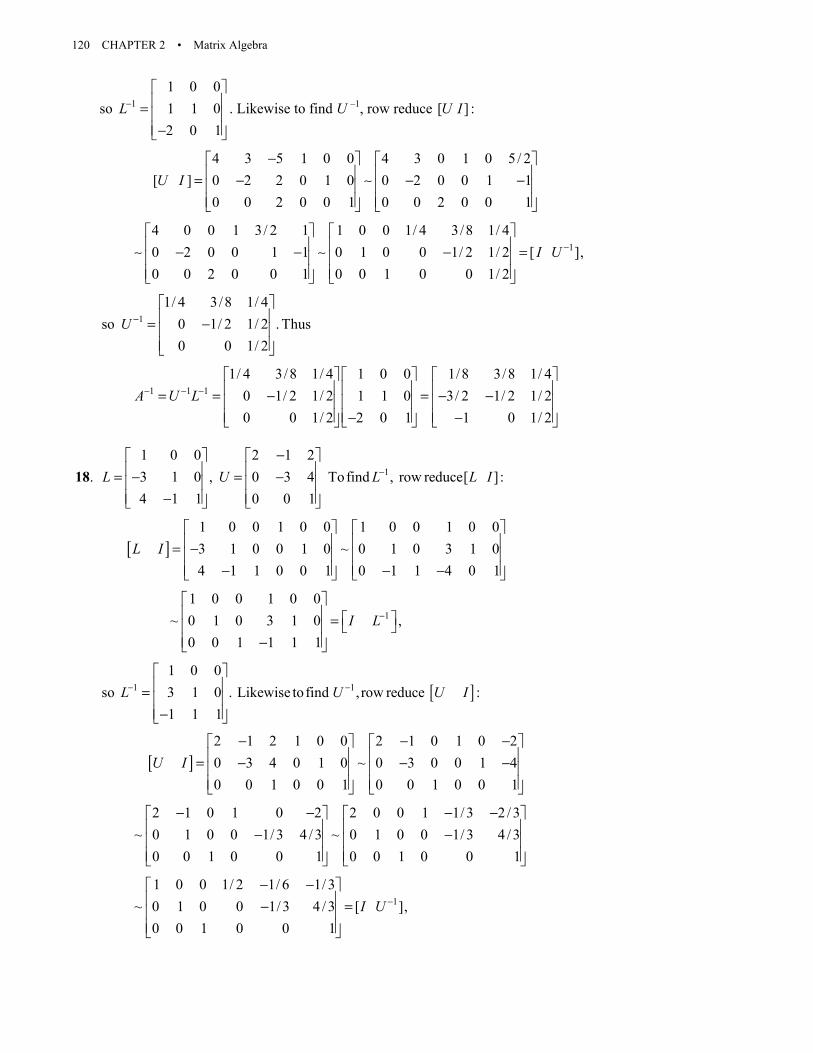
120 CHAPTER 2 • Matrix Algebra
so 11 0 01 1 02 0 1
L− = −
. Likewise to find U –1, row reduce [ ]U I :
4 3 5 1 0 0 4 3 0 1 0 5/ 2
[ ] 0 2 2 0 1 0 0 2 0 0 1 10 0 2 0 0 1 0 0 2 0 0 1
U I−
= − ∼ − −
14 0 0 1 3/ 2 1 1 0 0 1/ 4 3/8 1/ 40 2 0 0 1 1 0 1 0 0 1/ 2 1/ 2 [ ],0 0 2 0 0 1 0 0 1 0 0 1/ 2
I U − ∼ − − ∼ − =
11/ 4 3/8 1/ 4
so 0 1/ 2 1/ 2 . Thus0 0 1/ 2
U − = −
1 1 11/ 4 3/8 1/ 4 1 0 0 1/8 3/8 1/ 4
0 1/ 2 1/ 2 1 1 0 3/ 2 1/ 2 1/ 20 0 1/ 2 2 0 1 1 0 1/ 2
A U L− − − = = − = − − − −
18. 11 0 0 2 1 23 1 0 , 0 3 4 Tofind , row reduce[ ]:4 1 1 0 0 1
L U L L I−−
= − = − −
[ ]1 0 0 1 0 0 1 0 0 1 0 03 1 0 0 1 0 ~ 0 1 0 3 1 04 1 1 0 0 1 0 1 1 4 0 1
L I = − − − −
11 0 0 1 0 0
~ 0 1 0 3 1 0 ,0 0 1 1 1 1
I L− = −
[ ]1 11 0 0
so 3 1 0 . Likewise tofind , row reduce :1 1 1
L U U I− − = −
[ ]2 1 2 1 0 0 2 1 0 1 0 20 3 4 0 1 0 ~ 0 3 0 0 1 40 0 1 0 0 1 0 0 1 0 0 1
U I− − −
= − − −
2 1 0 1 0 2 2 0 0 1 1/ 3 2 / 3
~ 0 1 0 0 1/ 3 4 / 3 ~ 0 1 0 0 1/ 3 4 / 30 0 1 0 0 1 0 0 1 0 0 1
− − − − − −
11 0 0 1/ 2 1/ 6 1/ 3
~ 0 1 0 0 1/ 3 4 / 3 [ ],0 0 1 0 0 1
I U −− −
− =

2.5 • Solutions 121
11/ 2 1/ 6 1/ 3
so 0 1/ 3 4 / 3 . Thus0 0 1
U −− −
= −
1 1 11/ 2 1/ 6 1/ 3 1 0 0 1/ 3 1/ 2 1/ 3
0 1/3 4 /3 3 1 0 7 / 3 1 4 /30 0 1 1 1 1 1 1 1
A U L− − −− − − −
= = − = − − −
19. Let A be a lower-triangular n × n matrix with nonzero entries on the diagonal, and consider the augmented matrix [A I]. a. The (1, 1)-entry can be scaled to 1 and the entries below it can be changed to 0 by adding multiples
of row 1 to the rows below. This affects only the first column of A and the first column of I. So the (2, 2)-entry in the new matrix is still nonzero and now is the only nonzero entry of row 2 in the first n columns (because A was lower triangular).
The (2, 2)-entry can be scaled to 1, the entries below it can be changed to 0 by adding multiples of row 2 to the rows below. This affects only columns 2 and n + 2 of the augmented matrix. Now the (3, 3) entry in A is the only nonzero entry of the third row in the first n columns, so it can be scaled to 1 and then used as a pivot to zero out entries below it. Continuing in this way, A is eventually reduced to I, by scaling each row with a pivot and then using only row operations that add multiples of the pivot row to rows below.
b. The row operations just described only add rows to rows below, so the I on the right in [A I] changes into a lower triangular matrix. By Theorem 7 in Section 2.2, that matrix is A–1.
20. Let A = LU be an LU factorization for A. Since L is unit lower triangular, it is invertible by Exercise 19. Thus by the Invertible Matrix Theroem, L may be row reduced to I. But L is unit lower triangular, so it can be row reduced to I by adding suitable multiples of a row to the rows below it, beginning with the top row. Note that all of the described row operations done to L are row-replacement operations. If elementary matrices E1, E2, … Ep implement these row-replacement operations, then
2 1 2 1... ( ... )p pE E E A E E E LU IU U= = =
This shows that A may be row reduced to U using only row-replacement operations.
21. (Solution in Study Guide.) Suppose A = BC, with B invertible. Then there exist elementary matrices E1, …, Ep corresponding to row operations that reduce B to I, in the sense that Ep … E1B = I. Applying the same sequence of row operations to A amounts to left-multiplying A by the product Ep … E1. By associativity of matrix multiplication.
1 1... ...p pE E A E E BC IC C= = =
so the same sequence of row operations reduces A to C.
22. First find an LU factorization for A. Row reduce A to echelon form using only row replacement operations:
2 4 2 3 2 4 2 3 2 4 2 36 9 5 8 0 3 1 1 0 3 1 1
~ ~2 7 3 9 0 3 1 6 0 0 0 54 2 2 1 0 6 2 7 0 0 0 56 3 3 4 0 9 3 13 0 0 0 10
A
− − − − − − − − − − = − − − − − − − − − − − −

122 CHAPTER 2 • Matrix Algebra
2 4 2 30 3 1 1
~ 0 0 0 50 0 0 00 0 0 0
U
− − − =
then follow the algorithm in Example 2 to find L. Use the last two columns of I5 to make L unit lower triangular.
26 3
52 354 6
106 92 3 5
1 1 0 0 0 03 1 3 1 0 0 0
,1 1 1 1 1 1 0 02 2 1 1 2 2 1 1 03 3 2 0 1 3 3 2 0 1
L
− − − − ÷ ÷ ÷
=− − − − − − −
Now notice that the bottom two rows of U contain only zeros. If one uses the row-column method to find LU, the entries in the final two columns of L will not be used, since these entries will be multiplied zeros from the bottom two rows of U. So let B be the first three columns of L and let C be the top three rows of U. That is,
1 0 02 4 2 33 1 0
, 0 3 1 11 1 10 0 0 52 2 1
3 3 2
B C
− − = = −− − −
Then B and C have the desired sizes and BC = LU = A. We can generalize this process to the case where A in m × n, A = LU, and U has only three non-zero rows: let B be the first three columns of L and let C be the top three rows of U.
23. a. Express each row of D as the transpose of a column vector. Then use the multiplication rule for partitioned matrices to write
[ ]
1
21 41 2 3 4 1 2 2 3 43
3
4
T
TTT T T
T
T
A CD
= = = + + +
d
dc c c c c d c d c d c d
d
d
which is the sum of four outer products. b. Since A has 400 × 100 = 40000 entries, C has 400 × 4 = 1600 entries and D has 4 × 100 = 400 entries,
to store C and D together requires only 2000 entries, which is 5% of the amount of entries needed to store A directly.

2.5 • Solutions 123
24. Since Q is square and QTQ = I, Q is invertible by the Invertible Matrix Theorem and Q–1 = QT. Thus A is the product of invertible matrices and hence is invertible. Thus by Theorem 5, the equation Ax = b has a unique solution for all b. From Ax = b, we have QRx = b, QTQRx = QTb, Rx = QTb, and finally x = R–1QTb. A good algorithm for finding x is to compute QTb and then row reduce the matrix [ R QTb ]. See Exercise 11 in Section 2.2 for details on why this process works. The reduction is fast in this case because R is a triangular matrix.
25. A = UDV T . Since U and V T are square, the equations U T U = I and V T V = I imply that U and V T are invertible, by the IMT, and hence U– 1 = UT and (VT)–1 = V. Since the diagonal entries 1, , nσ σ… in D are nonzero, D is invertible, with the inverse of D being the diagonal matrix with 1 1
1 , ,n
σ σ− −… on the diagonal. Thus A is a product of invertible matrices. By Theorem 6, A is invertible and A–1 = (UDV T ) –1 = (VT)–1D–1U–1 = VD–1UT.
26. If A = PDP–1, where P is an invertible 3 × 3 matrix and D is the diagonal matrix
1 0 00 1/ 2 00 0 1/ 3
D =
then
2 1 1 1 1 1 2 1( )( ) ( )A PDP PDP PD P P DP PDIDP PD P− − − − − −= = = =
and since
2 2
2
1 0 01 0 0 1 0 0 1 0 00 1/ 2 0 0 1/ 2 0 0 1/ 2 0 0 1/ 4 00 0 1/ 3 0 0 1/ 3 0 0 1/ 90 0 1/ 3
D = = =
2 11 0 00 1/ 4 00 0 1/ 9
A P P− =
Likewise, A3 = PD3P –1, so
3 3 1 1
3
1 0 0 1 0 00 1/ 2 0 0 1/8 0
0 0 1/ 270 0 1/ 3
A P P P P− −
= =
In general, Ak = PDkP–1, so
1
1 0 0
0 1/ 2 0
0 0 1/ 3
k k
k
A P P−
=
27. First consider using a series circuit with resistance R1 followed by a shunt circuit with resistance R2 for the network. The transfer matrix for this network is
11
2 2 1 2 2
1 0 111/ 1 1/ ( ) /0 1
RRR R R R R
−− = − − +

124 CHAPTER 2 • Matrix Algebra
For an input of 12 volts and 6 amps to produce an output of 9 volts and 4 amps, the transfer matrix must satisfy
1 1
2 1 2 2 1 2 2
1 12 612 91/ ( )/ ( 12 6 6 )/6 4
R RR R R R R R R
− − = = − + − + +
Equate the top entries and obtain 11 2 ohm.R = Substitute this value in the bottom entry and solve to
obtain 92 2 ohms.R = The ladder network is
a. i2i1 i2 i3
v3v2v1
1/2 ohm9/2
ohms
Next consider using a shunt circuit with resistance R1 followed by a series circuit with resistance R2 for the network. The transfer matrix for this network is
1 2 1 22
1 1
1 0 ( )/11/ 1 1/ 10 1
R R R RRR R
+ −− = − −
For an input of 12 volts and 6 amps to produce an output of 9 volts and 4 amps, the transfer matrix must satisfy
1 2 1 2 1 2 1 2
1 1
( ) / (12 12 ) / 612 91/ 1 12 / 66 4
R R R R R R R RR R
+ − + − = = − − +
Equate the bottom entries and obtain R1 = 6 ohms. Substitute this value in the top entry and solve to obtain 3
2 4 ohms.R = The ladder network is
b. i2i1 i2 i3
3/4 ohmv3v2v1
6ohms
28. The three shunt circuits have transfer matrices
31 2
1 01 0 1 0, , and
1/ 11/ 1 1/ 1 RR R −− −
respectively. To find the transfer matrix for the series of circuits, multiply these matrices
3 1 2 32 1
1 0 1 01 0 1 0, , and
1/ 1 (1/ 1/ 1/ ) 11/ 1 1/ 1R R R RR R
= − − + +− −
Thus the resulting network is itself a shunt circuit with resistance 1 2 31/ 1/ 1/ .R R R+ +
29. a. The first circuit is a shunt circuit with resistance R1 ohms, so its transfer matrix is 1
1 01/ 1R
−
.
The second circuit is a series circuit with resistance R2 ohms, so its transfer matrix is 21.
0 1R−

2.5 • Solutions 125
The third circuit is a shunt circuit with resistance R3 ohms so its transfer matrix is 3
1 01/ 1R
−
.
The transfer matrix of the network is the product of these matrices, in right-to-left order:
2
3 1
1 0 1 011/ 1 1/ 10 1
RR R
− = − −
1 2 1 2
1 2 3 3 2 3 3
( ) /( ) / ( ) /
R R R RR R R R R R R
+ − − + + +
b. To find a ladder network with a structure like that in part (a) and with the given transfer matrix A, we must find resistances R1, R2, and R3 such that
1 2 1 2
1 2 3 3 2 3 3
( ) /4 / 3 12( ) / ( ) /1/ 4 3
R R R RA
R R R R R R R+ −−
= = − + + +−
From the (1, 2) entries, R2 = 12 ohms. The (1, 1) entries now give 1 1( 12) / 4 / 3,R R+ = which may be solved to obtain R1 = 36 ohms. Likewise the (2, 2) entries give 3 3( 12) / 3,R R+ = which also may be solved to obtain R3 = 6 ohms. Thus the matrix A may be factored as
2
3 1
1 0 1 011/ 1 1/ 10 1
RA
R R−
= − −
1 0 1 12 1 01/6 1 0 1 1/36 1
− = − −
The ladder network is
i2i1 i2 i3 i3 i4
v3 v4v2v136
ohms6
ohms
12 ohms
30. Answers may vary. The network below interchanges the series and shunt circuits.
i2i1 i2 i3 i3 i4
v3 v4v2v1
R1R2
R3
The transfer matrix of this network is the product of the individual transfer matrices, in right-to-left order.
3 1
2
1 01 11/ 10 1 0 1
R RR
− − = −
2 3 2 3 1 2 3 2
2 1 2 2
( ) / ( ) /1/ ( ) /
R R R R R R R RR R R R
+ − − + − +
By setting the matrix A from the previous exercise equal to this matrix, one may find that
2 3 2 3 1 2 3 2
2 1 2 2
( ) / ( ) / 4 /3 121/ ( ) / 1/4 3
R R R R R R R RR R R R
+ − − + − = − + −
Set the (2, 1) entries equal and obtain R2 = 4 ohms. Substitute this value for R2, equating the (2, 2) entries and solving gives R1 = 8 ohms. Likewise equating the (1, 1) entries gives R3 = 4/3 ohms.

126 CHAPTER 2 • Matrix Algebra
The ladder network is
i2i1 i2 i3 i3 i4
v3 v4v2v14
ohms
8 ohms 4/3 ohms
Note: The Study Guide’s MATLAB box for Section 2.5 suggests that for most LU factorizations in this section, students can use the gauss command repeatedly to produce U, and use paper and mental arithmetic to write down the columns of L as the row reduction to U proceeds. This is because for Exercises 7–16 the pivots are integers and other entries are simple fractions. However, for Exercises 31 and 32 this is not reasonable, and students are expected to solve an elementary programming problem. (The Study Guide provides no hints.)
31. [M] Store the matrix A in a temporary matrix B and create L initially as the 8×8 identity matrix. The following sequence of MATLAB commands fills in the entries of L below the diagonal, one column at a time, until the first seven columns are filled. (The eighth column is the final column of the identity matrix.)
L(2:8, 1) = B(2:8, 1)/B(1, 1) B = gauss(B, 1) L(3:8, 2) = B(3:8, 2)/B(2, 2) B = gauss(B, 2)
L(8:8, 7) = B(8:8, 7)/B(7, 7) U = gauss(B,7)
Of course, some students may realize that a loop will speed up the process. The for..end syntax is illustrated in the MATLAB box for Section 5.6. Here is a MATLAB program that includes the initial setup of B and L:
B = A L = eye(8) for j=1:7 L(j+1:8, j) = B(j+1:8, j)/B(j, j) B = gauss(B, j) end U = B
a. To four decimal places, the results of the LU decomposition are
1 0 0 0 0 0 0 0.25 1 0 0 0 0 0 0.25 .0667 1 0 0 0 0 00 .2667 .2857 1 0 0 0 00 0 .2679 .0833 1 0 0 00 0 0 .2917 .2921 1 0 00 0 0 0 .2697 .0861 1 00 0 0 0 0 .2948 .2931 1
L
− − − − − = − −
− − − −
− −

2.5 • Solutions 127
4 1 1 0 0 0 0 00 3.75 .25 1 0 0 0 00 0 3.7333 1.0667 1 0 0 00 0 0 3.4286 .2857 1 0 00 0 0 0 3.7083 1.0833 1 00 0 0 0 0 3.3919 .2921 10 0 0 0 0 0 3.7052 1.08610 0 0 0 0 0 0 3.3868
U
− − − − − − − − = − −
− − −
b. The result of solving Ly = b and then Ux = y is x = (3.9569, 6.5885, 4.2392, 7.3971, 5.6029, 8.7608, 9.4115, 12.0431)
c. 1
.2953 .0866 .0945 .0509 .0318 .0227 .0010 .0082
.0866 .2953 .0509 .0945 .0227 .0318 .0082 .0100
.0945 .0509 .3271 .1093 .1045 .0591 .0318 .0227
.0509 .0945 .1093 .3271 .0591 .1045 .0227 .0318
.0318 .0227 .1045 .0591 .3271 .1093 .0945 .A− =
0509.0227 .0318 .0591 .1045 .1093 .3271 .0509 .0945.0010 .0082 .0318 .0227 .0945 .0509 .2953 .0866.0082 .0100 .0227 .0318 .0509 .0945 .0866 .2953
32. [M]
3 1 0 0 01 3 1 0 00 1 3 1 00 0 1 3 10 0 0 1 3
A
− − − = − − − − −
. The commands shown for Exercise 31, but modified for 5×5
matrices, produce
13
38
821
2155
1 0 0 0 01 0 0 0
0 1 0 00 0 1 00 0 0 1
L
− −= − −
83
218
5521
14455
3 1 0 0 00 1 0 00 0 1 00 0 0 10 0 0 0
U
− − −= −

128 CHAPTER 2 • Matrix Algebra
b. Let sk+1 be the solution of Lsk+1 = tk for k = 0, 1, 2, …. Then tk+1 is the solution of Utk+1 = sk+1 for k = 0, 1, 2, …. The results are
1 1 2 2
10.0000 6.5556 6.5556 4.740715.3333 9.6667 11.8519 7.6667
, , ,17.7500 10.4444 14.8889 8.592618.7619 9.6667 15.3386 7.666717.1636 6.5556 12.4121 4.7407
= = = =
s t s t ,
3 3 4 4
4.7407 3.5988 3.5988 2.79229.2469 6.0556 7.2551 4.7778
, , ,12.0602 6.9012 9.6219 5.485612.2610 6.0556 9.7210 4.77789.4222 3.5988 7.3104 2.7922
= = = =
s t s t .
2.6 SOLUTIONS
Notes: This section is independent of Section 1.10. The material here makes a good backdrop for the series expansion of (I–C)–1 because this formula is actually used in some practical economic work. Exercise 8 gives an interpretation to entries of an inverse matrix that could be stated without the economic context.
1. The answer to this exercise will depend upon the order in which the student chooses to list the sectors. The important fact to remember is that each column is the unit consumption vector for the appropriate sector. If we order the sectors manufacturing, agriculture, and services, then the consumption matrix is
.10 .60 .60.30 .20 0.30 .10 .10
C =
The intermediate demands created by the production vector x are given by Cx. Thus in this case the intermediate demand is
.10 .60 .60 0 60.30 .20 .00 100 20.30 .10 .10 0 10
C = =
x
2. Solve the equation x = Cx + d for d:
1 1 1 2 3
2 2 1 2
3 3 1 2 3
.10 .60 .60 .9 .6 .6 0
.30 .20 .00 .3 .8 18
.30 .10 .10 .3 .1 .9 0
x x x x xC x x x x
x x x x x
− − = − = − = − + = − − +
d x x
This system of equations has the augmented matrix
.90 .60 .60 0 1 0 0 33.33.30 .80 .00 18 ~ 0 1 0 35.00.30 .10 .90 0 0 0 1 15.00
− − − − − −
so x = (33.33, 35.00, 15.00).

2.6 • Solutions 129
3. Solving as in Exercise 2:
1 1 1 2 3
2 2 1 2
3 3 1 2 3
.10 .60 .60 .9 .6 .6 18
.30 .20 .00 .3 .8 0
.30 .10 .10 .3 .1 .9 0
x x x x xx x x xx x x x x
− − = − = − = − + = − − +
d x xC
This system of equations has the augmented matrix
.90 .60 .60 18 1 0 0 40.00.30 .80 .00 0 ~ 0 1 0 15.00.30 .10 .90 0 0 0 1 15.00
− − − − −
so x = (40.00, 15.00, 15.00).
4. Solving as in Exercise 2:
1 1 1 2 3
2 2 1 2
3 3 1 2 3
.10 .60 .60 .9 .6 .6 18
.30 .20 .00 .3 .8 18
.30 .10 .10 .3 .1 .9 0
x x x x xC x x x x
x x x x x
− − = − = − = − + = − − +
d x x
This system of equations has the augmented matrix
.90 .60 .60 18 1 0 0 73.33.30 .80 .00 18 ~ 0 1 0 50.00.30 .10 .90 0 0 0 1 30.00
− − − − − −
so x = (73.33, 50.00, 30.00).
Note: Exercises 2–4 may be used by students to discover the linearity of the Leontief model.
5. 1
1 1 .5 50 1.6 1 50 110( )
.6 .8 20 1.2 2 20 120I C
−− −
= − = = = − x d
6. 1
1 .9 .6 18 40 / 21 30 / 21 18 50( )
.5 .8 11 25/ 21 45/ 21 11 45I C
−− −
= − = = = − x d
7. a. From Exercise 5,
1 1.6 1( )
1.2 2I C −
− =
so
11 1
1.6 1 1 1.6( )
1.2 2 0 1.2I C −
= − = =
x d
which is the first column of 1( ) .I C −−
b. 12 2
1.6 1 51 111.6( )
1.2 2 30 121.2I C −
= − = =
x d
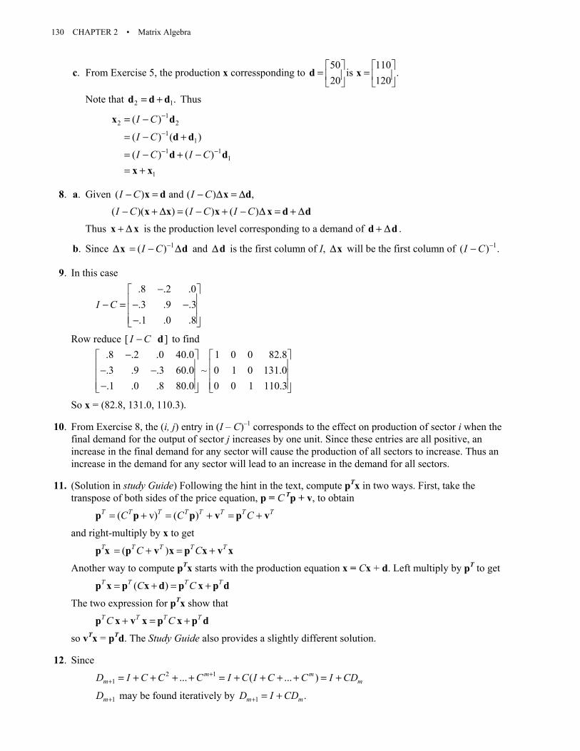
130 CHAPTER 2 • Matrix Algebra
c. From Exercise 5, the production x corressponding to 50 110
is .20 120
= =
d x
Note that 2 1.= +d d d Thus
12 2
11
1 11
1
( )
( ) ( )
( ) ( )
I C
I C
I C I C
−
−
− −
= −
= − +
= − + −= +
x d
d d
d dx x
8. a. Given ( ) and ( ) ,I C I C− = − =x d x d∆ ∆ ( )( ) ( ) ( )I C I C I C− + = − + − = +x x x x d d∆ ∆ ∆
Thus +x x∆ is the production level corresponding to a demand of .+d d∆
b. Since 1( )I C −= −x d∆ ∆ and d∆ is the first column of I, x∆ will be the first column of 1( )I C −− .
9. In this case
.8 .2 .0.3 .9 .3.1 .0 .8
I C−
− = − − −
Row reduce [ ]I C− d to find
.8 .2 .0 40.0 1 0 0 82.8.3 .9 .3 60.0 ~ 0 1 0 131.0.1 .0 .8 80.0 0 0 1 110.3
− − − −
So x = (82.8, 131.0, 110.3).
10. From Exercise 8, the (i, j) entry in (I – C)–1 corresponds to the effect on production of sector i when the final demand for the output of sector j increases by one unit. Since these entries are all positive, an increase in the final demand for any sector will cause the production of all sectors to increase. Thus an increase in the demand for any sector will lead to an increase in the demand for all sectors.
11. (Solution in study Guide) Following the hint in the text, compute pTx in two ways. First, take the transpose of both sides of the price equation, p = C Tp + v, to obtain
( v) ( )T T T T T T T TC C C= + = + = +p p p v p v
and right-multiply by x to get
( )T T T T TC C= + = +p x p v x p x v x
Another way to compute pTx starts with the production equation x = Cx + d. Left multiply by pT to get
( )T T T TC C= + = +p x p x d p x p d
The two expression for pTx show that
T T T TC C+ = +p x v x p x p d
so vTx = pTd. The Study Guide also provides a slightly different solution.
12. Since
2 11 ... ( ... )m m
m mD I C C C I C I C C I CD++ = + + + + = + + + + = +
1mD + may be found iteratively by 1 .m mD I CD+ = +

2.6 • Solutions 131
13. [M] The matrix I – C is
0.8412 0.0064 0.0025 0.0304 0.0014 0.0083 0.15940.0057 0.7355 0.0436 0.0099 0.0083 0.0201 0.34130.0264 0.1506 0.6443 0.0139 0.0142 0.0070 0.02360.3299 0.0565 0.0495 0.6364 0.0204 0.0483 0.06490.0089
− − − − − −− − − − − −− − − − − −− − − − − −− −0.0081 0.0333 0.0295 0.6588 0.0237 0.0020
0.1190 0.0901 0.0996 0.1260 0.1722 0.7632 0.33690.0063 0.0126 0.0196 0.0098 0.0064 0.0132 0.9988
− − − − − − − − − − − − − − − −
so the augmented matrix [ ]I C− d may be row reduced to find
0.8412 0.0064 0.0025 0.0304 0.0014 0.0083 0.1594 740000.0057 0.7355 0.0436 0.0099 0.0083 0.0201 0.3413 560000.0264 0.1506 0.6443 0.0139 0.0142 0.0070 0.0236 105000.3299 0.0565 0.0495 0.6364 0.0204 0.0483
− − − − − −− − − − − −− − − − − −− − − − − 0.0649 25000
0.0089 0.0081 0.0333 0.0295 0.6588 0.0237 0.0020 175000.1190 0.0901 0.0996 0.1260 0.1722 0.7632 0.3369 1960000.0063 0.0126 0.0196 0.0098 0.0064 0.0132 0.9988 5000
− − − − − − − − − − − − − − − − − − −
1 0 0 0 0 0 0 995760 1 0 0 0 0 0 977030 0 1 0 0 0 0 51231
~ 0 0 0 1 0 0 0 1315700 0 0 0 1 0 0 494880 0 0 0 0 1 0 3295540 0 0 0 0 0 1 13835
so x = (99576, 97703, 51321, 131570, 49488, 329554, 13835). Since the entries in d seem to be accurate to the nearest thousand, a more realistic answer would be x = (100000, 98000, 51000, 132000, 49000, 330000, 14000).
14. [M] The augmented matrix [ ]I C− d in this case may be row reduced to find
0.8412 0.0064 0.0025 0.0304 0.0014 0.0083 0.1594 996400.0057 0.7355 0.0436 0.0099 0.0083 0.0201 0.3413 755480.0264 0.1506 0.6443 0.0139 0.0142 0.0070 0.0236 144440.3299 0.0565 0.0495 0.6364 0.0204 0.0483
− − − − − −− − − − − −− − − − − −− − − − − 0.0649 33501
0.0089 0.0081 0.0333 0.0295 0.6588 0.0237 0.0020 235270.1190 0.0901 0.0996 0.1260 0.1722 0.7632 0.3369 2639850.0063 0.0126 0.0196 0.0098 0.0064 0.0132 0.9988 6526
− − − − − − − − − − − − − − − − − − −

132 CHAPTER 2 • Matrix Algebra
1 0 0 0 0 0 0 1340340 1 0 0 0 0 0 1316870 0 1 0 0 0 0 69472
~ 0 0 0 1 0 0 0 1769120 0 0 0 1 0 0 665960 0 0 0 0 1 0 4437730 0 0 0 0 0 1 18431
so x = (134034, 131687, 69472, 176912, 66596, 443773, 18431). To the nearest thousand, x = (134000, 132000, 69000, 177000, 67000, 444000, 18000).
15. [M] Here are the iterations rounded to the nearest tenth:
(0)
(1)
(2)
(3)
(74000.0, 56000.0, 10500.0, 25000.0, 17500.0, 196000.0, 5000.0)
(89344.2, 77730.5, 26708.1, 72334.7, 30325.6, 265158.2, 9327.8)
(94681.2, 87714.5, 37577.3, 100520.5, 38598.0, 296563.8, 11480.0)
(97091.
=
=
=
=
x
x
x
x(4)
(5)
(6)
9, 92573.1, 43867.8, 115457.0, 43491.0, 312319.0, 12598.8)
(98291.6, 95033.2, 47314.5, 123202.5, 46247.0, 320502.4, 13185.5)
(98907.2, 96305.3, 49160.6, 127213.7, 47756.4, 324796.1, 13493.8)
(99226.6, 96969.
=
=
=
x
x
x(7)
(8)
(9)
6, 50139.6, 129296.7, 48569.3, 327053.8, 13655.9)
(99393.1, 97317.8, 50656.4, 130381.6, 49002.8, 328240.9, 13741.1)
(99480.0, 97500.7, 50928.7, 130948.0, 49232.5, 328864.7, 13785.9)
(99525.5, 97596.8, 51071.
=
=
=
x
x
x(10)
(11)
(12)
9, 131244.1, 49353.8, 329192.3, 13809.4)
(99549.4, 97647.2, 51147.2, 131399.2, 49417.7, 329364.4, 13821.7)
(99561.9, 97673.7, 51186.8, 131480.4, 49451.3, 329454.7, 13828.2)
(99568.4, 97687.6, 51207.5, 131
=
=
=
x
x
x 523.0, 49469.0, 329502.1, 13831.6)
so x(12) is the first vector whose entries are accurate to the nearest thousand. The calculation of x(12) takes about 1260 flops, while the row reduction above takes about 550 flops. If C is larger than 20 20,× then fewer flops are required to compute x(12) by iteration than by row reduction. The advantage of the iterative method increases with the size of C. The matrix C also becomes more sparse for larger models, so fewer iterations are needed for good accuracy.
2.7 SOLUTIONS
Notes: The content of this section seems to have universal appeal with students. It also provides practice with composition of linear transformations. The case study for Chapter 2 concerns computer graphics – see this case study (available as a project on the website) for more examples of computer graphics in action. The Study Guide encourages the student to examine the book by Foley referenced in the text. This section could form the beginning of an independent study on computer graphics with an interested student.

2.7 • Solutions 133
1. Refer to Example 5. The representation in homogenous coordinates can be written as a partitioned matrix
of the form ,1T
A
0
0 where A is the matrix of the linear transformation. Since in this case
1 .25,
0 1A
=
the representation of the transformation with respect to homogenous coordinates is
1 .25 00 1 00 0 1
Note: The Study Guide shows the student why the action of 1T
A
0
0 on the vector
x1
corresponds to the
action of A on x.
2. The matrix of the transformation is 1 00 1
A−
=
, so the transformed data matrix is
1 0 5 2 4 5 2 40 1 0 2 3 0 2 3
AD− − − −
= =
Both the original triangle and the transformed triangle are shown in the following sketch.
–5 5x1
x2
2
3. Following Examples 4–6,
2 / 22 / 2 0 2 / 2 2 / 2 21 0 32 / 2 2 / 2 0 0 1 1 2 / 2 2 / 2 2 2
0 0 1 0 0 1 0 0 1
− − =
4. .8 0 0 1 0 2 .8 0 1.60 1.2 0 0 1 3 0 1.2 3.60 0 1 0 0 1 0 0 1
− − =
5.
3 / 2 1/ 2 0 3 / 2 1/ 2 01 0 01/ 2 3 / 2 0 0 1 0 1/ 2 3 / 2 0
0 0 1 0 0 1 0 0 1
− − = −
6.
3 / 2 1/ 2 0 3 / 2 1/ 2 01 0 00 1 0 1/ 2 3 / 2 0 1/ 2 3 / 2 00 0 1 0 0 1 0 0 1
− − − = − −

134 CHAPTER 2 • Matrix Algebra
7. A 60° rotation about the origin is given in homogeneous coordinates by the matrix 1/ 2 3 / 2 0
3 / 2 1/ 2 00 0 1
−
. To rotate about the point (6, 8), first translate by (–6, –8), then rotate about the
origin, then translate back by (6, 8) (see the Practice Problem in this section). A 60° rotation about (6, 8) is thus is given in homogeneous coordinates by the matrix
1/ 2 3 / 2 0 1/ 2 3 / 2 3 4 31 0 6 1 0 60 1 8 3 / 2 1/ 2 0 0 1 8 3 / 2 1/ 2 4 3 30 0 1 0 0 1 0 0 1 0 0 1
− − +− − = −
8. A 45° rotation about the origin is given in homogeneous coordinates by the matrix 2 / 2 2 / 2 0
2 / 2 2 / 2 00 0 1
−
. To rotate about the point (3, 7), first translate by (–3, –7), then rotate about the
origin, then translate back by (3, 7) (see the Practice Problem in this section). A 45° rotation about (3, 7) is thus is given in homogeneous coordinates by the matrix
2 / 2 2 / 2 0 2 / 2 2 / 2 3 2 21 0 3 1 0 30 1 7 2 / 2 2 / 2 0 0 1 7 2 / 2 2 / 2 7 5 20 0 1 0 0 1 0 0 1 0 0 1
− − +− − = −
9. To produce each entry in BD two multiplications are necessary. Since BD is a 2 200× matrix, it will take 2 2 200 800× × = multiplications to compute BD. By the same reasoning it will take 2 2 200× × = 800 multiplications to compute A(BD). Thus to compute A(BD) from the beginning will take 800 + 800 = 1600 multiplications.
To compute the 2 2× matrix AB it will take 2 2 2 8× × = multiplications, and to compute (AB)D it will take 2 2 200 800× × = multiplications. Thus to compute (AB)D from the beginning will take 8 + 800 = 808 multiplications.
For computer graphics calculations that require applying multiple transformations to data matrices, it is thus more efficient to compute the product of the transformation matrices before applying the result to the data matrix.
10. Let the transformation matrices in homogeneous coordinates for the dilation, rotation, and translation be called respectively D, and R, and T. Then for some value of s, ϕ, h, and k,
0 0 cos sin 0 1 0
0 0 , sin cos 0 , 0 10 0 1 0 0 1 0 0 1
s hD s R T k
ϕ ϕϕ ϕ
− = = =
Compute the products of these matrices:
cos sin 0 cos sin 0sin cos 0 , sin cos 00 0 1 0 0 1
s s s sDR s s RD s s
ϕ ϕ ϕ ϕϕ ϕ ϕ ϕ
− − = =

2.7 • Solutions 135
0 0
0 , 00 0 1 0 0 1
s sh s hDT s sk TD s k
= =
cos sin cos sin cos sinsin cos sin cos , sin cos
0 0 1 0 0 1
h k hRT h k TR k
ϕ ϕ ϕ ϕ ϕ ϕϕ ϕ ϕ ϕ ϕ ϕ
− − − = + =
Since DR = RD, DT ≠ TD and RT ≠ TR, D and R commute, D and T do not commute and R and T do not commute.
11. To simplify A2A1 completely, the following trigonometric identities will be needed:
1. sincostan cos cos sinϕ
ϕϕ ϕ ϕ ϕ− = − = −
2. 2 2sin 1 sin cos1
cos cos cos cossec tan sin sin cosϕ ϕ ϕϕ ϕ ϕ ϕϕ ϕ ϕ ϕ ϕ−− = − = = =
Using these identities,
2 1
sec tan 0 1 0 00 1 0 sin cos 00 0 1 0 0 1
A Aϕ ϕ
ϕ ϕ−
=
sec tan sin tan cos 0
sin cos 00 0 1
ϕ ϕ ϕ ϕ ϕϕ ϕ
− − =
cos sin 0sin cos 0
0 0 1
ϕ ϕϕ ϕ
− =
which is the transformation matrix in homogeneous coordinates for a rotation in 2.
12. To simplify this product completely, the following trigonometric identity will be needed:
1 cos sintan / 2sin 1 cos
ϕ ϕϕϕ ϕ
−= =+
This identity has two important consequences:
1 cos1 (tan / 2)(sin ) 1 sin cossin
ϕϕ ϕ ϕ ϕϕ
−− = − =
sin(cos )( tan / 2) tan / 2 (cos 1) tan / 2 (cos 1) sin1 cos
ϕϕ ϕ ϕ ϕ ϕ ϕ ϕϕ
− − = − + = − + = −+
The product may be computed and simplified using these results:
1 tan / 2 0 1 0 0 1 tan / 2 00 1 0 sin 1 0 0 1 00 0 1 0 0 1 0 0 1
ϕ ϕϕ
− −
1 (tan / 2)(sin ) tan / 2 0 1 tan / 2 0
sin 1 0 0 1 00 0 1 0 0 1
ϕ ϕ ϕ ϕϕ
− − − =

136 CHAPTER 2 • Matrix Algebra
cos tan / 2 0 1 tan / 2 0sin 1 0 0 1 0
0 0 1 0 0 1
ϕ ϕ ϕϕ
− − =
cos (cos )( tan / 2) tan / 2 0sin (sin )(tan / 2) 1 0
0 0 1
ϕ ϕ ϕ ϕϕ ϕ ϕ
− − = − +
cos sin 0sin cos 0
0 0 1
ϕ ϕϕ ϕ
− =
which is the transformation matrix in homogeneous coordinates for a rotation in 2.
13. Consider first applying the linear transformation on 2 whose matrix is A, then applying a translation by the vector p to the result. The matrix representation in homogeneous coordinates of the linear
transformation is ,1T
A
0
0 while the matrix representation in homogeneous coordinates of the
translation is .1T
I
p
0 Applying these transformations in order leads to a transformation whose matrix
representation in homogeneous coordinates is
1 1 1T T T
I A A =
p 0 p
0 0 0
which is the desired matrix.
14. The matrix for the transformation in Exercise 7 was found to be
1/ 2 3 / 2 3 4 3
3 / 2 1/ 2 4 3 30 0 1
− +
−
This matrix is of the form ,1T
A
p
0where
1/ 2 3 / 2 3 4 3
,3 / 2 1/ 2 4 3 3
A − +
= = −
p
By Exercise 13, this matrix may be written as
1 1T T
I A
p 0
0 0
that is, the composition of a linear transformation on 2 and a translation. The matrix A is the matrix of a rotation about the origin in 2. Thus the transformation in Exercise 7 is the composition of a rotation
about the origin and a translation by 3 4 3
.4 3 3
+=
− p

2.7 • Solutions 137
15. Since 1 1 1 12 4 8 24( , , , ) ( , , , ),X Y Z H = − the corresponding point in 3 has coordinates
11 182 4
1 1 124 24 24
( , , ) , , , , (12, 6,3)X Y Zx y zH H H
− = = = −
16. The homogeneous coordinates (1, –2, 3, 4) represent the point (1/ 4, 2 / 4, 3/ 4) (1/ 4, 1/ 2, 3/ 4)− = −
while the homogeneous coordinates (10, –20, 30, 40) represent the point (10 / 40, 20 / 40, 30 / 40) (1/ 4, 1/ 2, 3/ 4)− = −
so the two sets of homogeneous coordinates represent the same point in 3.
17. Follow Example 7a by first constructing that 3 3× matrix for this rotation. The vector e1 is not changed by this rotation. The vector e2 is rotated 60° toward the positive z-axis, ending up at the point (0, cos 60°, sin 60°) = (0, 1/ 2, 3 / 2). The vector e3 is rotated 60° toward the negative y-axis, stopping at the point (0, cos 150°, sin 150°) = (0, 3 / 2, 1/ 2).− The matrix A for this rotation is thus
1 0 0
0 1/ 2 3 / 2
0 3 / 2 1/ 2
A
= −
so in homogeneous coordinates the transformation is represented by the matrix
1 0 0 0
0 1/ 2 3 / 2 01 0 3 / 2 1/ 2 0
0 0 0 1
T
A
− =
0
0
18. First construct the 3 3× matrix for the rotation. The vector e1 is rotated 30° toward the negative y-axis, ending up at the point (cos(–30)°, sin (–30)°, 0) = ( 3 / 2, 1/ 2, 0).− The vector e2 is rotated 60° toward the positive x-axis, ending up at the point (cos 60°, sin 60°, 0) = (1/ 2, 3 / 2, 0). The vector e3 is not changed by the rotation. The matrix A for the rotation is thus
3 / 2 1/ 2 0
1/ 2 3 / 2 00 0 1
A
= −
so in homogeneous coordinates the rotation is represented by the matrix
3 / 2 1/ 2 0 0
1/ 2 3 / 2 0 01 0 0 1 0
0 0 0 1
T
A
− =
0
0
Following Example 7b, in homogeneous coordinates the translation by the vector (5, –2, 1) is represented by the matrix
1 0 0 50 1 0 20 0 1 10 0 0 1
−

138 CHAPTER 2 • Matrix Algebra
Thus the complete transformation is represented in homogeneous coordinates by the matrix
1 0 0 5 3 / 2 1/ 2 0 0 3 / 2 1/ 2 0 50 1 0 2 1/ 2 3 / 2 0 0 1/ 2 3 / 2 0 20 0 1 1 0 0 1 0 0 0 1 10 0 0 1 0 0 0 1 0 0 0 1
− − − − =
19. Referring to the material preceding Example 8 in the text, we find that the matrix P that performs a perspective projection with center of projection (0, 0, 10) is
1 0 0 00 1 0 00 0 0 00 0 .1 1
−
The homogeneous coordinates of the vertices of the triangle may be written as (4.2, 1.2, 4, 1), (6, 4, 2, 1), and (2, 2, 6, 1), so the data matrix for S is
4.2 6 21.2 4 2
4 2 61 1 1
and the data matrix for the transformed triangle is
1 0 0 0 4.2 6 2 4.2 6 20 1 0 0 1.2 4 2 1.2 4 20 0 0 0 4 2 6 0 0 00 0 .1 1 1 1 1 .6 .8 .4
= −
Finally, the columns of this matrix may be converted from homogeneous coordinates by dividing by the final coordinate:
(4.2, 1.2, 0, .6) (4.2 / .6, 1.2 / .6, 0 / .6) (7, 2, 0)(6, 4, 0, .8) (6 / .8, 2 / .8, 0 / .8) (7.5, 5, 0)(2, 2, 0, .4) (2 / .4, 2 / .4, 0 / .4) (5, 5, 0)
→ =→ =→ =
So the coordinates of the vertices of the transformed triangle are (7, 2, 0), (7.5, 5, 0), and (5, 5, 0).
20. As in the previous exercise, the matrix P that performs the perspective projection is
1 0 0 00 1 0 00 0 0 00 0 .1 1
−
The homogeneous coordinates of the vertices of the triangle may be written as (9, 3, –5, 1), (12, 8, 2, 1), and (1.8, 2.7, 1, 1), so the data matrix for S is
9 12 1.83 8 2.75 2 11 1 1
−

2.8 • Solutions 139
and the data matrix for the transformed triangle is
1 0 0 0 9 12 1.8 9 12 1.80 1 0 0 3 8 2.7 3 8 2.70 0 0 0 5 2 1 0 0 00 0 .1 1 1 1 1 1.5 .8 .9
= − −
Finally, the columns of this matrix may be converted from homogeneous coordinates by dividing by the final coordinate:
(9, 3, 0, 1.5) (9 /1.5, 3/1.5, 0 /1.5) (6, 2, 0)(12, 8, 0, .8) (12 /.8, 8 / .8, 0 / .8) (15, 10, 0)(1.8, 2.7, 0, .9) (1.8 / .9, 2.7 / .9, 0 / .9) (2, 3, 0)
→ =→ =→ =
So the coordinates of the vertices of the transformed triangle are (6, 2, 0), (15, 10, 0), and (2, 3, 0).
21. [M] Solve the given equation for the vector (R, G, B), giving
1.61 .29 .15 2.2586 1.0395 .3473.35 .59 .063 1.3495 2.3441 .0696.04 .12 .787 .0910 .3046 1.2777
R X XG Y YB Z Z
− − − = = − −
22. [M] Solve the given equation for the vector (R, G, B), giving
1.299 .587 .114 1.0031 .9548 .6179.596 .275 .321 .9968 .2707 .6448.212 .528 .311 1.0085 1.1105 1.6996
R Y YG I IB Q Q
− = − − = − − − −
2.8 SOLUTIONS
Notes: Cover this section only if you plan to skip most or all of Chapter 4. This section and the next cover everything you need from Sections 4.1–4.6 to discuss the topics in Section 4.9 and Chapters 5–7 (except for the general inner product spaces in Sections 6.7 and 6.8). Students may use Section 4.2 for review, particu-larly the Table near the end of the section. (The final subsection on linear transformations should be omitted.) Example 6 and the associated exercises are critical for work with eigenspaces in Chapters 5 and 7. Exercises 31–36 review the Invertible Matrix Theorem. New statements will be added to this theorem in Section 2.9.
Key Exercises: 5–20 and 23–26.
1. The set is closed under sums but not under multiplication by a negative scalar. A counterexample to the subspace condition is shown at the right.
Note: Most students prefer to give a geometric counterexample, but some may choose an algebraic calcu-lation. The four exercises here should help students develop an understanding of subspaces, but they may be insufficient if you want students to be able to analyze an unfamiliar set on an exam. Developing that skill seems more appropriate for classes covering Sections 4.1–4.6.
u
(–1)u

140 CHAPTER 2 • Matrix Algebra
2. The set is closed under scalar multiples but not sums. For example, the sum of the vectors u and v shown here is not in H.
3. No. The set is not closed under sums or scalar multiples. The subset consisting of the points on the line x2 = x1 is a subspace, so any “counterexample” must use at least one point not on this line. Here are two counterexamples to the subspace conditions:
4. No. The set is closed under sums, but not under multiplication by a negative scalar.
5. The vector w is in the subspace generated by v1 and v2 if and only if the vector equation x1v1 + x2v2 = w is consistent. The row operations below show that w is not in the subspace generated by v1 and v2.
1 2
2 4 8 2 4 8 2 4 8[ ] ~ 3 5 2 ~ 0 1 10 ~ 0 1 10
5 8 9 0 2 11 0 0 9
− − − − − − − − − −
v v w
6. The vector u is in the subspace generated by {v1, v2, v3} if and only if the vector equation x1v1 + x2v2 + x3v3 = u is consistent. The row operations below show that u is not in the subspace generated by {v1, v2, v3}.
1 2 3
1 4 5 4 1 4 5 4 1 4 5 42 7 8 10 0 1 2 2 0 1 2 2
[ ] ~ ~ ~4 9 6 7 0 7 14 9 0 0 0 233 7 5 5 0 5 10 7 0 0 0 17
− − − − − − − − − − − −
v v v u
Note: For a quiz, you could use w = (1, –3, 11, 8), which is in Span{v1, v2, v3}.
7. a. There are three vectors: v1, v2, and v3 in the set {v1, v2, v3}. b. There are infinitely many vectors in Span{v1, v2, v3} = Col A. c. Deciding whether p is in Col A requires calculation:
2 3 4 6 2 3 4 6 2 3 4 6
[ ] ~ 8 8 6 10 ~ 0 4 10 14 ~ 0 4 10 146 7 7 11 0 2 5 7 0 0 0 0
A− − − − − −
− − − − − − − − −
p
The equation Ax = p has a solution, so p is in Col A.
u
u + vv
u 3u
u + vv
u
(–1)u

2.8 • Solutions 141
8. 3 2 0 1 3 2 0 1 3 2 0 1
[ ] 0 2 6 14 ~ 0 2 6 14 ~ 0 2 6 146 3 3 9 0 1 3 7 0 0 0 0
A− − − − − − = − − − − − −
p
Yes, the augmented matrix [A p] corresponds to a consistent system, so p is in Col A.
9. To determine whether p is in Nul A, simply compute Ap. Using A and p as in Exercise 7,
Ap = 2 3 4 6 28 8 6 10 62 .6 7 7 11 29
− − − − − = − − −
Since Ap ≠ 0, p is not in Nul A.
10. To determine whether u is in Nul A, simply compute Au. Using A as in Exercise 7 and u = (–2, 3, 1),
Au = 3 2 0 2 00 2 6 3 0 .6 3 3 1 0
− − − − =
Yes, u is in Nul A.
11. p = 4 and q = 3. Nul A is a subspace of R4 because solutions of Ax = 0 must have 4 entries, to match the columns of A. Col A is a subspace of R3 because each column vector has 3 entries.
12. p = 3 and q = 4. Nul A is a subspace of R3 because solutions of Ax = 0 must have 3 entries, to match the columns of A. Col A is a subspace of R4 because each column vector has 4 entries.
13. To produce a vector in Col A, select any column of A. For Nul A, solve the equation Ax = 0. (Include an augmented column of zeros, to avoid errors.)
3 2 1 5 0 3 2 1 5 0 3 2 1 5 09 4 1 7 0 ~ 0 2 4 8 0 ~ 0 2 4 8 09 2 5 1 0 0 4 8 16 0 0 0 0 0 0
− − − − − − − − − −
3 2 1 5 0 1 0 1 1 0
~ 0 1 2 4 0 ~ 0 1 2 4 0 ,0 0 0 0 0 0 0 0 0 0
− − − −
1 3 4
2 3 4
02 4 0
0 0
x x xx x x
− + =+ − =
=
The general solution is x1 = x3 – x4, and x2 = –2x3 + 4x4, with x3 and x4 free. The general solution in parametric vector form is not needed. All that is required here is one nonzero vector. So choose any values for x3 and x4 (not both zero). For instance, set x3 = 1 and x4 = 0 to obtain the vector (1, –2, 1, 0) in Nul A.
Note: Section 2.8 of Study Guide introduces the ref command (or rref, depending on the technology), which produces the reduced echelon form of a matrix. This will greatly speed up homework for students who have a matrix program available.
14. To produce a vector in Col A, select any column of A. For Nul A, solve the equation Ax = 0:
1 2 3 0 1 2 3 0 1 2 3 0 1 0 1/ 3 04 5 7 0 0 3 5 0 0 1 5/ 3 0 0 1 5/ 3 0
~ ~ ~5 1 0 0 0 9 15 0 0 0 0 0 0 0 0 02 7 11 0 0 3 5 0 0 0 0 0 0 0 0 0
− − − − −
The general solution is x1 = (1/3)x3 and x2 = (–5/3) x3, with x3 free. The general solution in parametric vector form is not needed. All that is required here is one nonzero vector. So choose any values of x3 and x4 (not both zero). For instance, set x3 = 3 to obtain the vector (1, –5, 3) in Nul A.

142 CHAPTER 2 • Matrix Algebra
15. Yes. Let A be the matrix whose columns are the vectors given. Then A is invertible because its determinant is nonzero, and so its columns form a basis for R2, by the Invertible Matrix Theorem (or by Example 5). (Other reasons for the invertibility of A could be given.)
16. No. One vector is a multiple of the other, so they are linearly dependent and hence cannot be a basis for any subspace.
17. No. Place the three vectors into a 3×3 matrix A and determine whether A is invertible:
0 5 6 1 7 3 1 7 3 1 7 31 7 3 ~ 0 5 6 ~ 0 5 6 ~ 0 5 62 4 5 2 4 5 0 10 11 0 0 23
A− − −
= − − − −
The matrix A has three pivots, so A is invertible by the IMT and its columns form a basis for R3 (as pointed out in Example 5).
18. Yes. Place the three vectors into a 3×3 matrix A and determine whether A is invertible:
1 5 7 1 5 7 1 5 71 1 0 ~ 0 4 7 ~ 0 4 72 2 5 0 8 9 0 0 5
A− − −
= − − − − − − −
The matrix A has three pivots, so A is invertible by the IMT and its columns form a basis for R3 (as pointed out in Example 5).
19. No. The vectors cannot be a basis for R3 because they only span a plan in R3. Or, point out that the
columns of the matrix 1 51 12 2
− − −
cannot possibly span R3 because the matrix cannot have a pivot in
every row. So the columns are not a basis for R3.
Note: The Study Guide warns students not to say that the two vectors here are a basis for R2.
20. No. The vectors are linearly dependent because there are more vectors in the set than entries in each vector. (Theorem 8 in Section 1.7.) So the vectors cannot be a basis for any subspace.
21. a. False. See the definition at the beginning of the section. The critical phrases “for each” are missing. b. True. See the paragraph before Example 4. c. False. See Theorem 12. The null space is a subspace of Rn, not Rm. d. True. See Example 5. e. True. See the first part of the solution of Example 8.
22. a. False. See the definition at the beginning of the section. The condition about the zero vector is only one of the conditions for a subspace.
b. True. See Example 3. c. True. See Theorem 12. d. False. See the paragraph after Example 4. e. False. See the Warning that follows Theorem 13.

2.8 • Solutions 143
23. (Solution in Study Guide) 4 5 9 2 1 2 6 56 5 1 12 ~ 0 1 5 63 4 8 3 0 0 0 0
A− −
= − −
. The echelon form identifies
columns 1 and 2 as the pivot columns. A basis for Col A uses columns 1 and 2 of A: 4 56 , 53 4
. This is not
the only choice, but it is the “standard” choice. A wrong choice is to select columns 1 and 2 of the echelon form. These columns have zero in the third entry and could not possibly generate the columns displayed in A.
24. For Nul A, obtain the reduced (and augmented) echelon form for Ax = 0:
1 0 4 7 00 1 5 6 00 0 0 0 0
− −
. This corresponds to: 1 3 4
2 3 4
4 7 05 6 0
0 0
x x xx x x
− + =+ − =
=.
Solve for the basic variables and write the solution of Ax = 0 in parametric vector form:
1 3 4
2 3 43 4
3 3
4 4
4 7 4 75 6 5 6
1 00 1
x x xx x x
x xx xx x
− − − + − = = +
. Basis for Nul A:
4 75 6
,1 00 1
− −
Notes: (1) A basis is a set of vectors. For simplicity, the answers here and in the text list the vectors without enclosing the list inside set brackets. This style is also easier for students. I am careful, however, to distinguish between a matrix and the set or list whose elements are the columns of the matrix.
(2) Recall from Chapter 1 that students are encouraged to use the augmented matrix when solving Ax = 0, to avoid the common error of misinterpreting the reduced echelon form of A as itself the augmented matrix for a nonhomogeneous system.
(3) Because the concept of a basis is just being introduced, I insist that my students write the parametric vector form of the solution of Ax = 0. They see how the basis vectors span the solution space and are obviously linearly independent. A shortcut, which some instructors might introduce later in the course, is only to solve for the basic variables and to produce each basis vector one at a time. Namely, set all free variables equal to zero except for one free variable, and set that variable equal to a suitable nonzero number.
24. 3 9 2 7 1 3 6 92 6 4 8 ~ 0 0 4 53 9 2 2 0 0 0 0
A− − − − = − − −
. Basis for Col A: 3 22 , 43 2
− − −
.
For Nul A, obtain the reduced (and augmented) echelon form for Ax = 0:
1 3 0 1.50 00 0 1 1.25 00 0 0 0 0
−
. This corresponds to: 1 2 4
3 4
3 1.50 01.25 0
0 0
x x xx x
− + =+ =
=.
Solve for the basic variables and write the solution of Ax = 0 in parametric vector form:
1 2 4
2 22 4
3 4
4 4
3 1.5 3 1.51 0
1.25 0 1.250 1
x x xx x
x xx xx x
− − = = + − −
. Basis for Nul A:
3 1.51 0
,0 1.250 1
− −
.

144 CHAPTER 2 • Matrix Algebra
25.
1 4 8 3 7 1 4 8 0 51 2 7 3 4 0 2 5 0 1
~2 2 9 5 5 0 0 0 1 43 6 9 5 2 0 0 0 0 0
A
− − − − = − − −
. Basis for Col A:
1 4 31 2 3
, ,2 2 53 6 5
− − − −
.
For Nul A, obtain the reduced (and augmented) echelon form for Ax = 0:
1 0 2 0 7 00 1 2.5 0 .5 0
[ ] ~0 0 0 1 4 00 0 0 0 0 0
A
− −
0 .
1 3 5
2 3 5
4 5
2 7 02.5 .5 0
4 00 0
x x xx x x
x x
− + =+ − =
+ ==
.
1 3 5
2 3 5
3 53 3
4 5
5 5
2 7 2 72.5 .5 2.5 .5
Thesolution of 0in parametric vector form : .1 04 0 4
0 1
x x xx x x
A x xx xx xx x
− − − + − = = = + − −
x
u v
Basis for Nul A: {u, v}.
Note: The solution above illustrates how students could write a solution on an exam, when time is precious, namely, describe the basis by giving names to appropriate vectors found in the calculations.
26.
3 1 7 3 9 3 1 7 0 62 2 2 7 5 0 2 4 0 3
~5 9 3 3 4 0 0 0 1 12 6 6 3 7 0 0 0 0 0
A
− − − − = − −
. Basis for Col A:
3 1 32 2 7
, ,5 9 32 6 3
− − − −
.
For Nul A,
[ ]
1 0 3 0 2.5 00 1 2 0 1.5 0
~0 0 0 1 1 00 0 0 0 0 0
A
0 .
1 5
2 3 5
4 5
3 2.5 02 1.5 0
00 0
x x xx x x
x x
+ + =+ + =
+ ==
The solution of Ax = 0 in parametric vector form:
1 3 5
2 3 5
3 53 3
4 5
5 5
3 2.5 3 2.52 1.5 2 1.5
1 00 10 1
x x xx x x
x xx xx xx x
− − − − − − − − = = + − −
u v
. Basis for Nul A: {u, v}.
27. Construct a nonzero 3×3 matrix A and construct b to be almost any convenient linear combination of the columns of A.

2.8 • Solutions 145
28. The easiest construction is to write a 3×3 matrix in echelon form that has only 2 pivots, and let b be any vector in R3 whose third entry is nonzero.
29. (Solution in Study Guide) A simple construction is to write any nonzero 3×3 matrix whose columns are obviously linearly dependent, and then make b a vector of weights from a linear dependence relation among the columns. For instance, if the first two columns of A are equal, then b could be (1, –1, 0).
30. Since Col A is the set of all linear combinations of a1, … , ap, the set {a1, … , ap} spans Col A. Because {a1, … , ap} is also linearly independent, it is a basis for Col A. (There is no need to discuss pivot columns and Theorem 13, though a proof could be given using this information.)
31. If Col F ≠ R5, then the columns of F do not span R5. Since F is square, the IMT shows that F is not invertible and the equation Fx = 0 has a nontrivial solution. That is, Nul F contains a nonzero vector. Another way to describe this is to write Nul F ≠ {0}.
32. If Nul R contains nonzero vectors, then the equation Rx = 0 has nontrivial solutions. Since R is square, the IMT shows that R is not invertible and the columns of R do not span R6. So Col R is a subspace of R6, but Col R ≠ R6.
33. If Col Q = R4, then the columns of Q span R4. Since Q is square, the IMT shows that Q is invertible and the equation Qx = b has a solution for each b in R4. Also, each solution is unique, by Theorem 5 in Section 2.2.
34. If Nul P = {0}, then the equation Px = 0 has only the trivial solution. Since P is square, the IMT shows that P is invertible and the equation Px = b has a solution for each b in R5. Also, each solution is unique, by Theorem 5 in Section 2.2.
35. If the columns of B are linearly independent, then the equation Bx = 0 has only the trivial (zero) solution. That is, Nul B = {0}.
36. If the columns of A form a basis, they are linearly independent. This means that A cannot have more columns than rows. Since the columns also span Rm, A must have a pivot in each row, which means that A cannot have more rows than columns. As a result, A must be a square matrix.
37. [M] Use the command that produces the reduced echelon form in one step (ref or rref depending on the program). See the Section 2.8 in the Study Guide for details. By Theorem 13, the pivot columns of A form a basis for Col A.
3 5 0 1 3 1 0 2.5 4.5 3.57 9 4 9 11 0 1 1.5 2.5 1.5
~5 7 2 5 7 0 0 0 0 03 7 3 4 0 0 0 0 0 0
A
− − − − − − − = − − − − −
Basis for Col A:
3 57 9
,5 73 7
− − − −
For Nul A, obtain the solution of Ax = 0 in parametric vector form:
1 3 4 5
2 3 4 5
2.5 4.5 3.5 01.5 2.5 1.5 0
x x x xx x x x
+ − + =+ − + =
Solution: 1 3 4 5
2 3 4 5
3 4 5
2.5 4.5 3.51.5 2.5 1.5
, , and are free
x x x xx x x xx x x
= − + − = − + −

146 CHAPTER 2 • Matrix Algebra
1 3 4 5
2 3 4 5
3 4 53 3
4 4
5 5
2.5 4.5 3.5 2.5 4.5 3.51.5 2.5 1.5 1.5 2.5 1.5
1 0 00 1 00 0 1
x x x xx x x x
x x xx xx xx x
− + − − − − + − − − = = = + +
x = x3u + x4v + x5w
By the argument in Example 6, a basis for Nul A is {u, v, w}.
38. [M]
5 2 0 8 8 1 0 0 60 1224 1 2 8 9 0 1 0 154 309
~5 1 3 5 19 0 0 1 47 948 5 6 8 5 0 0 0 0 0
A
− − − − − − = − − − −
.
The pivot columns of A form a basis for Col A:
5 2 04 1 2
, ,5 1 38 5 6
− −
.
For Nul A, solve Ax = 0: 1 4 5
2 4 5
3 4 5
60 122 0154 309 047 94 0
x x xx x x
x x x
+ + =− − =− − =
Solution:
1 4 5
2 4 5
3 4 5
4 5
60 122154 30947 94
and are free
x x xx x xx x xx x
= − − = + = +
1 4 5
2 4 5
4 53 4 5
4 4
5 5
60 122 60 122154 309 154 309
47 94 47 941 00 1
x x xx x x
x xx x xx xx x
− − − − + = = = ++
x = x4u + x5v
By the method of Example 6, a basis for Nul A is {u, v}
Note: The Study Guide for Section 2.8 gives directions for students to construct a review sheet for the concept of a subspace and the two main types of subspaces, Col A and Nul A, and a review sheet for the concept of a basis. I encourage you to consider making this an assignment for your class.
2.9 SOLUTIONS
Notes: This section contains the ideas from Sections 4.4–4.6 that are needed for later work in Chapters 5–7. If you have time, you can enrich the geometric content of “coordinate systems” by discussing crystal lattices (Example 3 and Exercises 35 and 36 in Section 4.4.) Some students might profit from reading Examples 1–3 from Section 4.4 and Examples 2, 4, and 5 from Section 4.6. Section 4.5 is probably not a good reference for students who have not considered general vector spaces.
Coordinate vectors are important mainly to give an intuitive and geometric feeling for the isomorphism between a k-dimensional subspace and Rk. If you plan to omit Sections 5.4, 5.6, 5.7 and 7.2, you can safely omit Exercises 1–8 here.

2.9 • Solutions 147
Exercises 1–16 may be assigned after students have read as far as Example 2. Exercises 19 and 20 use the Rank Theorem, but they can also be assigned before the Rank Theorem is discussed.
The Rank Theorem in this section omits the nontrivial fact about Row A which is included in the Rank Theorem of Section 4.6, but that is used only in Section 7.4. The row space itself can be introduced in Section 6.2, for use in Chapter 6 and Section 7.4.
Exercises 9–16 include important review of techniques taught in Section 2.8 (and in Sections 1.2 and 2.5). They make good test questions because they require little arithmetic. My students need the practice here. Nearly every time I teach the course and start Chapter 5, I find that at least one or two students cannot find a basis for a two-dimensional eigenspace!
1. If [x]B = 32
, then x is formed from b1 and b2 using
weights 3 and 2:
x = 3b1 + 2b2 = 1 2 7
3 21 1 1
+ = −
2. If [x]B = 13
−
, then x is formed from b1 and b2 using weights –1 and 3:
x = (–1)b1 + 3b2 = 2 3 11
( 1) 31 1 2
− − + =
3. To find c1 and c2 that satisfy x = c1b1 + c2b2, row reduce the augmented matrix:
1 21 2 3 1 2 3 1 0 7
[ ] ~ ~4 7 7 0 1 5 0 1 5
− − − − = − − −
b b x . Or, one can write a matrix equation as
suggested by Exercise 7 and solve using the matrix inverse. In either case,
[x]B = 1
2
7.
5cc
=
4. As in Exercise 3, 1 21 3 7 1 3 7 1 0 5
[ ] ~ ~3 5 5 0 4 16 0 1 4
− − − − = − − −
b b x , and
[x]B = 1
2
5.
4cc
=
5. 1 2
1 3 4 1 3 4 1 0 1/ 4[ ] 5 7 10 ~ 0 8 10 ~ 0 1 5/ 4
3 5 7 0 4 5 0 0 0
− − = − − − − − −
b b x . [x]B = 1
2
1/ 4.
5 / 4cc
= −
b2
2b2
b1
2b1
3b1
xx1
x2
b2
2b2
b1
3b2
–b1
x
x1
x2

148 CHAPTER 2 • Matrix Algebra
6. 1 2
3 7 11 1 5 0 1 0 5/ 2[ ] 1 5 0 ~ 0 22 11 ~ 0 1 1/ 2
4 6 7 0 14 7 0 0 0
− − = − −
b b x
[x]B = 1
2
5 / 2.
1/ 2cc
− =
7. Fig. 1 suggests that w = 2b1 – b2 and x = 1.5b1 + .5b2, in which case,
[w]B = 21
−
and [x]B = 1.5.5
. To confirm [x]B, compute
1 23 1 4
1.5 .5 1.5 .50 2 1
− + = + = =
b b x
Figure 1 Figure 2
Note: Figures 1 and 2 display what Section 4.4 calls B-graph paper.
8. Fig. 2 suggests that x = 2b1 – b2, y = 1.5b1 + b2, and z = –b1 – .5b2. If so, then
[x]B = 21
−
, [y]B = 1.51.0
, and [z]B = 1.5
− −
. To confirm [y]B and [z]B, compute
1 20 2 2
1.5 1.52 1 4
+ = + = =
b b y and 1 2
0 2 1.5 1 .5
2 1 2.5−
− − = − − = = − b b z .
9. The information
1 3 2 4 1 3 2 43 9 1 5 0 0 5 7
~2 6 4 3 0 0 0 54 12 2 7 0 0 0 0
A
− − − − − − − = − − −
is enough to see that columns 1, 3, and 4 of
A form a basis for Col A:
1 2 43 1 5
, , .2 4 34 2 7
− − − − −
Columns 1, 2 and 4, of the echelon form certain cannot span Col A since those vectors all have zero in their fourth entries. For Nul A, use the reduced echelon form, augmented with a zero column to insure that the equation Ax = 0 is kept in mind:
b 2
b1
x
w
0
b2
b1
x
0
z
y

2.9 • Solutions 149
1 3 0 0 00 0 1 0 00 0 0 1 00 0 0 0 0
−
.
1 2
3
4
2
3 000
is the free variable
x xx
xx
− ===
, x =
1 2
2 22
3
4
3 31
.0 00 0
x xx x
xxx
= =
So
3100
is
a basis for Nul A. From this information, dim Col A = 3 (because A has three pivot columns) and dim Nul A = 1 (because the equation Ax = 0 has only one free variable).
10. The information
1 2 9 5 4 1 2 9 5 41 1 6 5 3 0 1 3 0 7
~2 0 6 1 2 0 0 0 1 24 1 9 1 9 0 0 0 0 0
A
− − − − − − = − − − − −
shows that columns 1, 2,
and 4 of A form a basis for Col A:
1 2 51 1 5
, ,2 0 14 1 1
− − −
. For Nul A,
[ ]
1 0 3 0 0 00 1 3 0 7 0
~0 0 0 1 2 00 0 0 0 0 0
A
− − −
0 .
1 3
2 3 5
4 5
3 5
3 03 7 0
2 0and are free variables
x xx x x
x xx x
+ =− − =
− =
1 3
2 3 5
3 53 3
4 5
5 5
3 3 03 7 3 7
.1 02 0 2
0 1
x xx x x
x xx xx xx x
− − + = = = +
x Basis for Nul A:
3 03 7
,1 00 20 1
−
.
From this, dim Col A = 3 and dim Nul A = 2.
11. The information
1 2 5 0 1 1 2 5 0 12 5 8 4 3 0 1 2 4 5
~3 9 9 7 2 0 0 0 1 23 10 7 11 7 0 0 0 0 0
A
− − − − − = − − − − −
shows that columns 1, 2,
and 4 of A form a basis for Col A:
1 2 02 5 4
, , .3 9 73 10 11
− − −
For Nul A,
[ ]
1 0 9 0 5 00 1 2 0 3 0
~ .0 0 0 1 2 00 0 0 0 0 0
A
− −
0
1 3 5
2 3 5
4 5
3 5
9 5 02 3 0
2 0and are free variables
x x xx x x
x xx x
− + =+ − =
+ =

150 CHAPTER 2 • Matrix Algebra
1 3 5
2 3 5
3 53 3
4 5
5 5
9 5 9 52 3 2 3
.1 02 0 2
0 1
x x xx x x
x xx xx xx x
− − − + − = = = + − −
x Basis for Nul A:
9 52 3
, .1 00 20 1
− − −
From this, dim Col A = 3 and dim Nul A = 2.
12. The information
1 2 4 3 3 1 2 4 3 35 10 9 7 8 0 0 1 2 0
~4 8 9 2 7 0 0 0 0 52 4 5 0 6 0 0 0 0 0
A
− − − − − = − − − − − −
shows that columns 1, 3,
and 5 of A form a basis for Col A:
1 4 35 9 8
, , .4 9 72 5 6
− − − − −
For Nul A
[ ]
1 2 0 5 0 00 0 1 2 0 0
~ .0 0 0 0 1 00 0 0 0 0 0
A
− −
0
1 2 4
3 4
5
2 4
2 5 02 0
0and are free variables
x x xx x
xx x
+ − =− =
=
1 2 4
2 2
2 43 4
4 4
5
2 5 2 51 0
.2 0 20 1
0 0 0
x x xx x
x xx xx xx
− + − = = = +
x Basis for Nul A:
2 51 0
, .0 20 10 0
−
From this, dim Col A = 3 and dim Nul A = 2.
13. The four vectors span the column space H of a matrix that can be reduced to echelon form:
1 3 2 4 1 3 2 4 1 3 2 4 1 3 2 43 9 1 5 0 0 5 7 0 0 5 7 0 0 5 7
~ ~ ~2 6 4 3 0 0 0 5 0 0 0 5 0 0 0 54 12 2 7 0 0 10 9 0 0 0 5 0 0 0 0
− − − − − − − − − − − − − − − − −
Columns 1, 3, and 4 of the original matrix form a basis for H, so dim H = 3.
Note: Either Exercise 13 or 14 should be assigned because there are always one or two students who confuse Col A with Nul A. Or, they wrongly connect “set of linear combinations” with “parametric vector form” (of the general solution of Ax = 0).
14. The five vectors span the column space H of a matrix that can be reduced to echelon form:
1 2 0 1 3 1 2 0 1 3 1 2 0 1 31 3 2 4 8 0 1 2 3 5 0 1 2 3 5
~ ~2 1 6 7 9 0 3 6 9 15 0 0 0 0 05 6 8 7 5 0 4 8 12 20 0 0 0 0 0
− − − − − − − − − − − − − − − − − − −
Columns 1 and 2 of the original matrix form a basis for H, so dim H = 2.

2.9 • Solutions 151
15. Col A = R3, because A has a pivot in each row and so the columns of A span R3. Nul A cannot equal R2, because Nul A is a subspace of R5. It is true, however, that Nul A is two-dimensional. Reason: the equation Ax = 0 has two free variables, because A has five columns and only three of them are pivot columns.
16. Col A cannot be R3 because the columns of A have four entries. (In fact, Col A is a 3-dimensional subspace of R4, because the 3 pivot columns of A form a basis for Col A.) Since A has 7 columns and 3 pivot columns, the equation Ax = 0 has 4 free variables. So, dim Nul A = 4.
17. a. True. This is the definition of a B-coordinate vector. b. False. Dimension is defined only for a subspace. A line must be through the origin in Rn to be a
subspace of Rn. c. True. The sentence before Example 1 concludes that the number of pivot columns of A is the rank of
A, which is the dimension of Col A by definition. d. True. This is equivalent to the Rank Theorem because rank A is the dimension of Col A. e. True, by the Basis Theorem. In this case, the spanning set is automatically a linearly independent set.
18. a. True. This fact is justified in the second paragraph of this section. b. True. See the second paragraph after Fig. 1. c. False. The dimension of Nul A is the number of free variables in the equation Ax = 0.
See Example 2. d. True, by the definition of rank. e. True, by the Basis Theorem. In this case, the linearly independent set is automatically a spanning set.
19. The fact that the solution space of Ax = 0 has a basis of three vectors means that dim Nul A = 3. Since a 5×7 matrix A has 7 columns, the Rank Theorem shows that rank A = 7 – dim Nul A = 4.
Note: One can solve Exercises 19–22 without explicit reference to the Rank Theorem. For instance, in Exercise 19, if the null space of a matrix A is three-dimensional, then the equation Ax = 0 has three free variables, and three of the columns of A are nonpivot columns. Since a 5×7 matrix has seven columns, A must have four pivot columns (which form a basis of Col A). So rank A = dim Col A = 4.
20. A 4×5 matrix A has 5 columns. By the Rank Theorem, rank A = 5 – dim Nul A. Since the null space is three-dimensional, rank A = 2.
21. A 7×6 matrix has 6 columns. By the Rank Theorem, dim Nul A = 6 – rank A. Since the rank is four, dim Nul A = 2. That is, the dimension of the solution space of Ax = 0 is two.
22. The wording of this problem was poor in the first printing, because the phrase “it spans a four-dimensional subspace” was never defined. Here is a revision that I will put in later printings of the third edition:
Show that a set {v1, …, v5} in Rn is linearly dependent if dim Span{v1, …, v5} = 4. Solution: Suppose that the subspace H = Span{v1, …, v5} is four-dimensional. If {v1, …, v5} were
linearly independent, it would be a basis for H. This is impossible, by the statement just before the definition of dimension in Section 2.9, which essentially says that every basis of a p-dimensional subspace consists of p vectors. Thus, {v1, …, v5} must be linearly dependent.
23. A 3×4 matrix A with a two-dimensional column space has two pivot columns. The remaining two columns will correspond to free variables in the equation Ax = 0. So the desired construction is possible.

152 CHAPTER 2 • Matrix Algebra
There are six possible locations for the two pivot columns, one of which is * * *
0 * *0 0 0 0
. A simple
construction is to take two vectors in R3 that are obviously not linearly dependent, and put two copies of these two vectors in any order. The resulting matrix will obviously have a two-dimensional column space. There is no need to worry about whether Nul A has the correct dimension, since this is guaranteed by the Rank Theorem: dim Nul A = 4 – rank A.
24. A rank 1 matrix has a one-dimensional column space. Every column is a multiple of some fixed vector. To construct a 4×3 matrix, choose any nonzero vector in R4, and use it for one column. Choose any multiples of the vector for the other two columns.
25. The p columns of A span Col A by definition. If dim Col A = p, then the spanning set of p columns is automatically a basis for Col A, by the Basis Theorem. In particular, the columns are linearly independent.
26. If columns a1, a3, a5, and a6 of A are linearly independent and if dim Col A = 4, then {a1, a3, a5, a6} is a linearly independent set in a 4-dimensional column space. By the Basis Theorem, this set of four vectors is a basis for the column space.
27. a. Start with B = [b1 ⋅ ⋅ ⋅ bp] and A = [a1 ⋅ ⋅ ⋅ aq], where q > p. For j = 1, …, q, the vector aj is in W. Since the columns of B span W, the vector aj is in the column space of B. That is, aj = Bcj for some vector cj of weights. Note that cj is in Rp because B has p columns.
b. Let C = [c1 ⋅ ⋅ ⋅ cq]. Then C is a p×q matrix because each of the q columns is in Rp. By hypothesis, q is larger than p, so C has more columns than rows. By a theorem, the columns of C are linearly dependent and there exists a nonzero vector u in Rq such that Cu = 0.
c. From part (a) and the definition of matrix multiplication A = [a1 ⋅ ⋅ ⋅ aq] = [Bc1 ⋅ ⋅ ⋅ Bcq] = BC From part (b), Au = (BC)u = B(Cu) = B0 = 0. Since u is nonzero, the columns of A are linearly
dependent.
28. If A contained more vectors than B, then A would be linearly dependent, by Exercise 27, because B spans W. Repeat the argument with B and A interchanged to conclude that B cannot contain more vectors than A.
29. [M] Apply the matrix command ref or rref to the matrix [v1 v2 x]:
11 14 19 1 0 1.6675 8 13 0 1 2.667
~10 13 18 0 0 07 10 15 0 0 0
− − − −
The equation c1v1 + c2v2 = x is consistent, so x is in the subspace H. The decimal approximations suggest c1 = –5/3 and c2 = 8/3, and it can be checked that these values are precise. Thus, the B-coordinate of x is (–5/3, 8/3).
30. [M] Apply the matrix command ref or rref to the matrix [v1 v2 v3 x]:
6 8 9 4 1 0 0 34 3 5 7 0 1 0 5
~9 7 8 8 0 0 1 24 3 3 3 0 0 0 0
− − − − − − −

Chapter 2 • Supplementary Exercises 153
The first three columns of [v1 v2 v3 x] are pivot columns, so v1, v2 and v3 are linearly independent. Thus v1, v2 and v3 form a basis B for the subspace H which they span. View [v1 v2 v3 x] as an augmented matrix for c1v1 + c2v2 + c3v3 = x. The reduced echelon form shows that x is in H and
[x]B = 35 .2
Notes: The Study Guide for Section 2.9 contains a complete list of the statements in the Invertible Matrix Theorem that have been given so far. The format is the same as that used in Section 2.3, with three columns: statements that are logically equivalent for any m×n matrix and are related to existence concepts, those that are equivalent only for any n×n matrix, and those that are equivalent for any n×p matrix and are related to uniqueness concepts. Four statements are included that are not in the text’s official list of statements, to give more symmetry to the three columns.
The Study Guide section also contains directions for making a review sheet for “dimension” and “rank.”
Chapter 2 SUPPLEMENTARY EXERCISES
1. a. True. If A and B are m×n matrices, then BT has as many rows as A has columns, so ABT is defined. Also, ATB is defined because AT has m columns and B has m rows.
b. False. B must have 2 columns. A has as many columns as B has rows. c. True. The ith row of A has the form (0, …, di, …, 0). So the ith row of AB is (0, …, di, …, 0)B, which
is di times the ith row of B. d. False. Take the zero matrix for B. Or, construct a matrix B such that the equation Bx = 0 has
nontrivial solutions, and construct C and D so that C ≠ D and the columns of C – D satisfy the equation Bx = 0. Then B(C – D) = 0 and BC = BD.
e. False. Counterexample: A = 1 00 0
and C = 0 00 1
.
f. False. (A + B)(A – B) = A2 – AB + BA – B2. This equals A2 – B2 if and only if A commutes with B. g. True. An n×n replacement matrix has n + 1 nonzero entries. The n×n scale and interchange matrices
have n nonzero entries. h. True. The transpose of an elementary matrix is an elementary matrix of the same type. i. True. An n×n elementary matrix is obtained by a row operation on In. j. False. Elementary matrices are invertible, so a product of such matrices is invertible. But not every
square matrix is invertible. k. True. If A is 3×3 with three pivot positions, then A is row equivalent to I3. l. False. A must be square in order to conclude from the equation AB = I that A is invertible. m. False. AB is invertible, but (AB)–1 = B–1A–1, and this product is not always equal to A–1B–1. n. True. Given AB = BA, left-multiply by A–1 to get B = A–1BA, and then right-multiply by A–1 to obtain
BA–1 = A–1B. o. False. The correct equation is (rA)–1 = r–1A–1, because
(rA)(r–1A–1) = (rr–1)(AA–1) = 1⋅I = I.
p. True. If the equation Ax = 100
has a unique solution, then there are no free variables in this equation,
which means that A must have three pivot positions (since A is 3×3). By the Invertible Matrix Theorem, A is invertible.

154 CHAPTER 2 • Matrix Algebra
2. C = (C– 1)–1 = 7 5 7 / 2 5/ 216 4 3 22
− − = − −−
3. 20 0 0 0 0 0 0 0 0 0 0 01 0 0 , 1 0 0 1 0 0 0 0 00 1 0 0 1 0 0 1 0 1 0 0
A A = = =
3 20 0 0 0 0 0 0 0 01 0 0 0 0 0 0 0 00 1 0 1 0 0 0 0 0
A A A = ⋅ = =
Next, 2 2 2 2 2 3 3( )( ) ( )I A I A A I A A A I A A I A A A A A I A− + + = + + − + + = + + − − − = − .
Since A3 = 0, 2( )( )I A I A A I− + + = .
4. From Exercise 3, the inverse of I – A is probably I + A + A2 + ⋅ ⋅ ⋅ + An–1. To verify this, compute
1 1 1 1( )( ) ( )n n n n nI A I A A I A A A I A A I AA I A− − − −− + + + = + + + − + + + = − = −
If An = 0, then the matrix B = I + A + A2 + ⋅ ⋅ ⋅ + An–1 satisfies (I – A)B = I. Since I – A and B are square, they are invertible by the Invertible Matrix Theorem, and B is the inverse of I – A.
5. A2 = 2A – I. Multiply by A: A3 = 2A2 – A. Substitute A2 = 2A – I: A3 = 2(2A – I) – A = 3A – 2I. Multiply by A again: A4 = A(3A – 2I) = 3A2 – 2A. Substitute the identity A2 = 2A – I again:
Finally, A4 = 3(2A – I) – 2A = 4A – 3I.
6. Let 1 0 0 1
and .0 1 1 0
A B
= = − By direct computation, A2 = I, B2 = I, and AB =
0 11 0
−
= – BA.
7. (Partial answer in Study Guide) Since A–1B is the solution of AX = B, row reduction of [A B] to [I X] will produce X = A–1B. See Exercise 12 in Section 2.2.
[ ]1 3 8 3 5 1 3 8 3 5 1 3 8 3 52 4 11 1 5 ~ 0 2 5 7 5 ~ 0 1 3 6 11 2 5 3 4 0 1 3 6 1 0 2 5 7 5
A B− − −
= − − − − − − − − − −
1 3 8 3 5 1 3 0 37 29 1 0 0 10 1
~ 0 1 3 6 1 ~ 0 1 0 9 10 ~ 0 1 0 9 100 0 1 5 3 0 0 1 5 3 0 0 1 5 3
− − − − − − − − −
Thus, A–1B = 10 1
9 105 3
− − −
.
8. By definition of matrix multiplication, the matrix A satisfies
1 2 1 33 7 1 1
A
=

Chapter 2 • Supplementary Exercises 155
Right-multiply both sides by the inverse of 1 23 7
. The left side becomes A. Thus,
1 3 7 2 2 11 1 3 1 4 1
A− −
= = − −
9. Given 5 4 7 3
and 2 3 2 1
AB B
= = − , notice that ABB–1 = A. Since det B = 7 – 6 =1,
1 11 3 5 4 1 3 3 13 and ( )
2 7 2 3 2 7 8 27B A AB B− −− − −
= = = = − − − −
Note: Variants of this question make simple exam questions.
10. Since A is invertible, so is AT, by the Invertible Matrix Theorem. Then ATA is the product of invertible matrices and so is invertible. Thus, the formula (ATA)–1AT makes sense. By Theorem 6 in Section 2.2,
(ATA)–1⋅AT = A–1(AT)–1AT = A–1I = A–1
An alternative calculation: (ATA)–1AT⋅A = (ATA)–1(ATA) = I. Since A is invertible, this equation shows that its inverse is (ATA)–1AT.
11. a. For i = 1,…, n, p(xi) = c0 + c1xi + ⋅ ⋅ ⋅ + 11
ninc x −
− = 0
1
row ( ) row ( )
n
i i
cV V
c −
⋅ =
c .
By a property of matrix multiplication, shown after Example 6 in Section 2.1, and the fact that c was chosen to satisfy Vc= y,
row ( ) row ( ) row ( )i ii iV V y= = =c c y
Thus, p(xi) = yi. To summarize, the entries in Vc are the values of the polynomial p(x) at x1, …, xn. b. Suppose x1, …, xn are distinct, and suppose Vc = 0 for some vector c. Then the entries in c are the
coefficients of a polynomial whose value is zero at the distinct points x1, ..., xn. However, a nonzero polynomial of degree n – 1 cannot have n zeros, so the polynomial must be identically zero. That is, the entries in c must all be zero. This shows that the columns of V are linearly independent.
c. (Solution in Study Guide) When x1, …, xn are distinct, the columns of V are linearly independent, by (b). By the Invertible Matrix Theorem, V is invertible and its columns span Rn. So, for every y = (y1, …, yn) in Rn, there is a vector c such that Vc = y. Let p be the polynomial whose coefficients are listed in c. Then, by (a), p is an interpolating polynomial for (x1, y1), …, (xn, yn).
12. If A = LU, then col1(A) = L⋅col1(U). Since col1(U) has a zero in every entry except possibly the first,
L⋅col1(U) is a linear combination of the columns of L in which all weights except possibly the first are zero. So col1(A) is a multiple of col1(L).
Similarly, col2(A) = L⋅col2(U), which is a linear combination of the columns of L using the first two entries in col2(U) as weights, because the other entries in col2(U) are zero. Thus col2(A) is a linear combination of the first two columns of L.
13. a. P2 = (uuT)(uuT) = u(uTu)uT = u(1)uT = P, because u satisfies uTu = 1. b. PT = (uuT)T = uTTuT = uuT = P c. Q2 = (I – 2P)(I – 2P) = I – I(2P) – 2PI + 2P(2P) = I – 4P + 4P2 = I, because of part (a).

156 CHAPTER 2 • Matrix Algebra
14. Given 001
=
u , define P and Q as in Exercise 13 by
[ ]0 0 0 0 1 0 0 0 0 0 1 0 00 0 0 1 0 0 0 , 2 0 1 0 2 0 0 0 0 1 01 0 0 1 0 0 1 0 0 1 0 0 1
TP Q I P = = = = − = − = −
uu
If 153
=
x , then0 0 0 1 0 1 0 0 1 10 0 0 5 0 and 0 1 0 5 50 0 1 3 3 0 0 1 3 3
P Q = = = = − −
x x .
15. Left-multiplication by an elementary matrix produces an elementary row operation: 1 2 1 3 2 1~ ~ ~B E B E E B E E E B C=
so B is row equivalent to C. Since row operations are reversible, C is row equivalent to B. (Alternatively, show C being changed into B by row operations using the inverse of the Ei .)
16. Since A is not invertible, there is a nonzero vector v in Rn such that Av = 0. Place n copies of v into an n×n matrix B. Then AB = A[v ⋅ ⋅ ⋅ v] = [Av ⋅ ⋅ ⋅ Av] = 0.
17. Let A be a 6×4 matrix and B a 4×6 matrix. Since B has more columns than rows, its six columns are linearly dependent and there is a nonzero x such that Bx = 0. Thus ABx = A0 = 0. This shows that the matrix AB is not invertible, by the IMT. (Basically the same argument was used to solve Exercise 22 in Section 2.1.)
Note: (In the Study Guide) It is possible that BA is invertible. For example, let C be an invertible 4×4 matrix
and construct 1 and [ 0].0C
A B C− = =
Then BA = I4, which is invertible.
18. By hypothesis, A is 5×3, C is 3×5, and AC = I3. Suppose x satisfies Ax = b. Then CAx = Cb. Since CA = I, x must be Cb. This shows that Cb is the only solution of Ax = b.
19. [M] Let .4 .2 .3.3 .6 .3.3 .2 .4
A =
. Then 2.31 .26 .30.39 .48 .39.30 .26 .31
A =
. Instead of computing A3 next, speed up the
calculations by computing
4 2 2 8 4 4.2875 .2834 .2874 .2857 .2857 .2857.4251 .4332 .4251 , .4285 .4286 .4285.2874 .2834 .2875 .2857 .2857 .2857
A A A A A A = = = =
To four decimal places, as k increases,
.2857 .2857 .2857.4286 .4286 .4286.2857 .2857 .2857
kA →
, or, in rational format, 2 / 7 2 / 7 2 / 73/ 7 3/ 7 3/ 72 / 7 2 / 7 2 / 7
kA →
.

Chapter 2 • Supplementary Exercises 157
If 20 .2 .3 .29 .18 .18.1 .6 .3 , then .33 .44 .33.9 .2 .4 .38 .38 .49
B B = =
,
4 8.2119 .1998 .1998 .2024 .2022 .2022.3663 .3764 .3663 , .3707 .3709 .3707.4218 .4218 .4339 .4269 .4269 .4271
B B = =
To four decimal places, as k increases,
.2022 .2022 .2022.3708 .3708 .3708.4270 .4270 .4270
kB →
, or, in rational format, 18/89 18/89 18/8933/89 33/89 33/8938/89 38/89 38/89
kB →
.
20. [M] The 4×4 matrix A4 is the 4×4 matrix of ones, minus the 4×4 identity matrix. The MATLAB command is A4 = ones(4) – eye(4). For the inverse, use inv(A4).
14 4
0 1 1 1 2 / 3 1/ 3 1/ 3 1/ 31 0 1 1 1/ 3 2 / 3 1/ 3 1/ 3
,1 1 0 1 1/ 3 1/ 3 2 / 3 1/ 31 1 1 0 1/ 3 1/ 3 1/ 3 2 / 3
A A−
− − = = − −
15 5
0 1 1 1 1 3/ 4 1/ 4 1/ 4 1/ 4 1/ 41 0 1 1 1 1/ 4 3/ 4 1/ 4 1/ 4 1/ 4
,1 1 0 1 1 1/ 4 1/ 4 3/ 4 1/ 4 1/ 41 1 1 0 1 1/ 4 1/ 4 1/ 4 3/ 4 1/ 41 1 1 1 0 1/ 4 1/ 4 1/ 4 1/ 4 3/ 4
A A−
− − = = − − −
16 6
0 1 1 1 1 1 4 / 5 1/ 5 1/ 5 1/ 5 1/ 5 1/ 51 0 1 1 1 1 1/ 5 4 / 5 1/ 5 1/ 5 1/ 5 1/ 51 1 0 1 1 1 1/ 5 1/ 5 4 / 5 1/ 5 1/ 5 1/ 5
,1 1 1 0 1 1 1/ 5 1/ 5 1/5 4 /5 1/5 1/ 51 1 1 1 0 1 1/ 5 1/ 5 1/ 5 1/ 5 4 / 5 1/ 51 1 1 1 1 0 1/ 5 1/ 5 1/ 5 1/ 5 1/ 5 4 / 5
A A−
− − −
= = − −
−
The construction of A6 and the appearance of its inverse suggest that the inverse is related to I6. In fact, 1
6 6A I− + is 1/5 times the 6×6 matrix of ones. Let J denotes the n×n matrix of ones. The conjecture is:
An = J – In and 1 11n nA J I
n− = ⋅ −
−
Proof: (Not required) Observe that J 2 = nJ and An J = (J – I ) J = J 2 – J = (n – 1) J. Now compute An((n – 1)–1J – I) = (n – 1)–1A n J – An = J – (J – I) = I Since An is square, An is invertible and its inverse is (n – 1)–1J – I.


159
3.1 SOLUTIONS
Notes: Some exercises in this section provide practice in computing determinants, while others allow the student to discover the properties of determinants which will be studied in the next section. Determinants are developed through the cofactor expansion, which is given in Theorem 1. Exercises 33–36 in this section provide the first step in the inductive proof of Theorem 3 in the next section.
1. Expanding along the first row:
3 0 4
3 2 2 2 2 32 3 2 3 0 4 3( 13) 4(10) 1
5 1 0 1 0 50 5 1
= − + = − + =− −
−
Expanding along the second column:
1 2 2 2 3 23 0 4
2 2 3 4 3 42 3 2 ( 1) 0 ( 1) 3 ( 1) 5 3( 3) 5( 2) 1
0 1 0 1 2 20 5 1
+ + += − ⋅ + − ⋅ + − ⋅ = − − − =− −
−
2. Expanding along the first row:
0 5 1
3 0 4 0 4 34 3 0 0 5 1 5(4) 1(22) 2
4 1 2 1 2 42 4 1
− −− = − + = − + =
Expanding along the second column:
1 2 2 2 3 20 5 1
4 0 0 1 0 14 3 0 ( 1) 5 ( 1) ( 3) ( 1) 4 5(4) 3( 2) 4( 4) 2
2 1 2 1 4 02 4 1
+ + +− = − ⋅ + − ⋅ − + − ⋅ = − − − − − =
3. Expanding along the first row:
2 4 3
1 2 3 2 3 13 1 2 2 ( 4) 3 2( 9) 4( 5) (3)(11) 5
4 1 1 1 1 41 4 1
−= − − + = − + − + = −
− −−

160 CHAPTER 3 • Determinants
Expanding along the second column:
1 2 2 2 3 22 4 3
3 2 2 3 2 33 1 2 ( 1) ( 4) ( 1) 1 ( 1) 4 4( 5) 1( 5) 4( 5) 5
1 1 1 1 3 21 4 1
+ + +−
= − ⋅ − + − ⋅ + − ⋅ = − + − − − = −− −
−
4. Expanding along the first row:
1 3 5
1 1 2 1 2 12 1 1 1 3 5 1( 2) 3(1) 5(5) 20
4 2 3 2 3 43 4 2
= − + = − − + =
Expanding along the second column:
1 2 2 2 3 21 3 5
2 1 1 5 1 52 1 1 ( 1) 3 ( 1) 1 ( 1) 4 3(1) 1( 13) 4( 9) 20
3 2 3 2 2 13 4 2
+ + += − ⋅ + − ⋅ + − ⋅ = − + − − − =
5. Expanding along the first row:
2 3 4
0 5 4 5 4 04 0 5 2 3 ( 4) 2( 5) 3( 1) 4(4) 23
1 6 5 6 5 15 1 6
−= − + − = − − − − = −
6. Expanding along the first row:
5 2 4
3 5 0 5 0 30 3 5 5 ( 2) 4 5(1) 2(10) 4( 6) 1
4 7 2 7 2 42 4 7
−− −
− = − − + = + + − =− −
−
7. Expanding along the first row:
4 3 0
5 2 6 2 6 56 5 2 4 3 0 4(1) 3(0) 4
7 3 9 3 9 79 7 3
= − + = − =
8. Expanding along the first row:
8 1 6
0 3 4 3 4 04 0 3 8 1 6 8(6) 1(11) 6( 8) 11
2 5 3 5 3 23 2 5
= − + = − + − = −− −
−
9. First expand along the third row, then expand along the first row of the remaining matrix:
3 1 1 3
6 0 0 50 0 5
1 7 2 5 7 2( 1) 2 7 2 5 2 ( 1) 5 10(1) 10
2 0 0 0 3 13 1 8
8 3 1 8
+ +−= − ⋅ − = ⋅ − ⋅ = =

3.1 • Solutions 161
10. First expand along the second row, then expand along either the third row or the second column of the remaining matrix.
2 3
1 2 5 21 2 2
0 0 3 0( 1) 3 2 6 5
2 6 7 55 0 4
5 0 4 4
+
−−
= − ⋅ −− −
3 1 3 32 2 1 2( 3) ( 1) 5 ( 1) 4 ( 3)(5(2) 4( 2)) 6
6 5 2 6+ + − −
= − − ⋅ + − ⋅ = − + − = − − −
or
2 3
1 2 5 21 2 2
0 0 3 0( 1) 3 2 6 5
2 6 7 55 0 4
5 0 4 4
+
−−
= − ⋅ −− −
1 2 2 22 5 1 2( 3) ( 1) ( 2) ( 1) ( 6)
5 4 5 4+ +
= − − ⋅ − + − ⋅ −
( )( 3) 2( 17) 6( 6) 6= − − − − = −
11. There are many ways to do this determinant efficiently. One strategy is to always expand along the first column of each matrix:
1 1 1 1
3 5 8 42 3 7
0 2 3 7 1 5( 1) 3 0 1 5 3 ( 1) ( 2)
0 0 1 5 0 20 0 2
0 0 0 2
+ +
−− −
− −= − ⋅ = ⋅ − ⋅ − = 3(–2)(2) = –12
12. There are many ways to do this determinant efficiently. One strategy is to always expand along the first row of each matrix:
1 1 1 1
4 0 0 01 0 0
7 1 0 0 3 0( 1) 4 6 3 0 4 ( 1) ( 1)
2 6 3 0 4 38 4 3
5 8 4 3
+ +−
−= − ⋅ = ⋅ − ⋅ −
−− −
− −
= 4(–1)( –9) = 36
13. First expand along either the second row or the second column. Using the second row,
2 3
4 0 7 3 54 0 3 5
0 0 2 0 07 3 4 8
( 1) 27 3 6 4 85 0 2 3
5 0 5 2 30 0 1 2
0 0 9 1 2
+
− −−−
= − ⋅− −−
−−
−
Now expand along the second column to find:
2 3 2 2
4 0 3 54 3 5
7 3 4 8( 1) 2 2 ( 1) 3 5 2 3
5 0 2 30 1 2
0 0 1 2
+ +
− −
− − ⋅ = − − ⋅ − − − −

162 CHAPTER 3 • Determinants
Now expand along either the first column or third row. The first column is used below.
2 24 3 5
2 ( 1) 3 5 2 30 1 2
+ − − − ⋅ − −
1 1 2 12 3 3 56 ( 1) 4 ( 1) 5 ( 6)(4(1) 5(1)) 6
1 2 1 2+ + − −
= − − ⋅ + − ⋅ = − − = − −
14. First expand along either the fourth row or the fifth column. Using the fifth column,
3 5
6 3 2 4 06 3 2 4
9 0 4 1 09 0 4 1
( 1) 18 5 6 7 13 0 0 0
3 0 0 0 04 2 3 2
4 2 3 2 0
+−
−= − ⋅−
Now expand along the third row to find:
3 5 3 1
6 3 2 43 2 4
9 0 4 1( 1) 1 1 ( 1) 3 0 4 1
3 0 0 02 3 2
4 2 3 2
+ +
− − ⋅ = − ⋅ −
Now expand along either the first column or second row. The first column is used below.
3 13 2 4
1 ( 1) 3 0 4 12 3 2
+ − ⋅ −
1 1 3 14 1 2 43 ( 1) 3 ( 1) 2 (3)(3( 11) 2(18)) 9
3 2 4 1+ + −
= − ⋅ + − ⋅ = − + = −
15. 3 0 42 3 20 5 1
=−
(3)(3)(–1) + (0)(2)(0) + (4)(2)(5) – (0)(3)(4) – (5)(2)(3) – (–1)(2)(0) =
–9 + 0 + 40 – 0 – 30 –0 = 1
16. 0 5 14 3 02 4 1
− = (0)(–3)(1) + (5)(0)(2) + (1)(4)(4) – (2)(–3)(1) – (4)(0)(0) – (1)(4)(5) =
0 + 0 + 16 – (–6) – 0 – 20 = 2
17. 2 4 33 1 21 4 1
−=
− (2)(1)(–1) + (–4)(2)(1) + (3)(3)(4) – (1)(1)(3) – (4)(2)(2) – (–1)(3)(–4) =
–2 + (–8) + 36 – 3 – 16 – 12 = –5
18. 1 3 52 1 13 4 2
= (1)(1)(2) + (3)(1)(3) + (5)(2)(4) – (3)(1)(5) – (4)(1)(1) – (2)(2)(3) =
2 + 9 + 40 – 15 – 4 – 12 = 20

3.1 • Solutions 163
19. ,a b
ad bcc d
= − ( )c d
cb da ad bca b
= − = − −
The row operation swaps rows 1 and 2 of the matrix, and the sign of the determinant is reversed.
20. ,a b
ad bcc d
= − ( ) ( ) ( )a b
a kd kc b kad kbc k ad bckc kd
= − = − = −
The row operation scales row 2 by k, and the determinant is multiplied by k.
21. 3 4
18 20 2,5 6
= − = − 3 4
3(6 4 ) (5 3 )4 25 3 6 4
k kk k
= + − + = −+ +
The row operation replaces row 2 with k times row 1 plus row 2, and the determinant is unchanged.
22. ,a b
ad bcc d
= − ( ) ( )a kc b kd
a kc d c b kd ad kcd bc kcd ad bcc d+ +
= + − + = + − − = −
The row operation replaces row 1 with k times row 2 plus row 1, and the determinant is unchanged.
23. 1 1 13 8 4 1(4) 1(2) 1( 7) 5,2 3 2
− − = − + − = −−
3 8 4 (4) (2) ( 7) 52 3 2
k k kk k k k− − = − + − = −
−
The row operation scales row 1 by k, and the determinant is multiplied by k.
24. 3 2 2 (2) (6) (3) 2 6 3 ,6 5 6
a b ca b c a b c= − + = − +
3 2 2
3(6 5 ) 2(6 6 ) 2(5 6 ) 2 6 36 5 6a b c b c a c a b a b c= − − − + − = − + −
The row operation swaps rows 1 and 2 of the matrix, and the sign of the determinant is reversed.
25. Since the matrix is triangular, by Theorem 2 the determinant is the product of the diagonal entries:
1 0 00 1 0 (1)(1)(1) 10 1k
= =
26. Since the matrix is triangular, by Theorem 2 the determinant is the product of the diagonal entries:
1 0 00 1 0 (1)(1)(1) 1
0 1k= =
27. Since the matrix is triangular, by Theorem 2 the determinant is the product of the diagonal entries:
0 0
0 1 0 ( )(1)(1)0 0 1
kk k= =

164 CHAPTER 3 • Determinants
28. Since the matrix is triangular, by Theorem 2 the determinant is the product of the diagonal entries:
1 0 00 0 (1)( )(1)0 0 1
k k k= =
29. A cofactor expansion along row 1 gives
0 1 0
1 01 0 0 1 1
0 10 0 1
= − = −
30. A cofactor expansion along row 1 gives
0 0 1
0 10 1 0 1 1
1 01 0 0
= = −
31. A 3 × 3 elementary row replacement matrix looks like one of the six matrices
1 0 0 1 0 0 1 0 0 1 0 0 1 0 1 0
1 0 , 0 1 0 , 0 1 0 , 0 1 k , 0 1 0 , 0 1 00 0 1 0 1 0 1 0 0 1 0 0 1 0 0 1
k kk
k k
In each of these cases, the matrix is triangular and its determinant is the product of its diagonal entries, which is 1. Thus the determinant of a 3 × 3 elementary row replacement matrix is 1.
32. A 3 × 3 elementary scaling matrix with k on the diagonal looks like one of the three matrices
0 0 1 0 0 1 0 0
0 1 0 , 0 0 , 0 1 00 0 1 0 0 1 0 0
kk
k
In each of these cases, the matrix is triangular and its determinant is the product of its diagonal entries, which is k. Thus the determinant of a 3 × 3 elementary scaling matrix with k on the diagonal is k.
33. 0 1
,1 0
E
=
,a b
Ac d
=
c dEA
a b
=
det E = –1, det A = ad – bc, det EA = cb – da = –1(ad – bc) = (det E)(det A)
34. 1 0
,0
Ek
=
,a b
Ac d
=
a bEA
kc kd
=
det E = k, det A = ad – bc, det EA = a(kd) – (kc)b = k(ad – bc) = (det E)(det A)
35. 1
,0 1
kE
=
,a b
Ac d
=
a kc b kdEA
c d+ +
=
det E = 1, det A = ad – bc, det EA = (a + kc)d – c(b + kd) = ad + kcd – bc – kcd = 1(ad – bc) = (det E)(det A)

3.1 • Solutions 165
36. 1 0
,1
Ek
=
,a b
Ac d
=
a bEA
ka c kb d
= + +
det E = 1, det A = ad – bc, det EA = a(kb + d) – (ka + c)b = kab + ad – kab – bc = 1(ad – bc) = (det E)(det A)
37. 3 1
,4 2
A
=
15 5
5 ,20 10
A
=
det A = 2, det 5A = 50 ≠ 5det A
38. ,a b
Ac d
=
,ka kb
kAkc kd
=
det A = ad – bc,
2 2det ( )( ) ( )( ) ( ) detkA ka kd kb kc k ad bc k A= − = − =
39. a. True. See the paragraph preceding the definition of the determinant. b. False. See the definition of cofactor, which precedes Theorem 1.
40. a. False. See Theorem 1. b. False. See Theorem 2.
41. The area of the parallelogram determined by 3
,0
=
u 1
,2
=
v u + v, and 0 is 6, since the base of the
parallelogram has length 3 and the height of the parallelogram is 2. By the same reasoning, the area of
the parallelogram determined by 3
,0
=
u ,2x
=
x u + x, and 0 is also 6.
X
V
U U
X2
X2
X1 X1
2
1 2
1
1 12 24
Also note that [ ] 3 1det det 6,
0 2
= =
u v and [ ] 3det det 6.
0 2x
= =
u x The determinant of the
matrix whose columns are those vectors which define the sides of the parallelogram adjacent to 0 is equal to the area of the parallelogram.
42. The area of the parallelogram determined by ab
=
u , 0c
=
v , u + v, and 0 is cb, since the base of the
parallelogram has length c and the height of the parallelogram is b.
X2
a
b
cX1
U
V

166 CHAPTER 3 • Determinants
Also note that [ ]det det0
a ccb
b
= = −
u v , and [ ]det det .0c a
cbb
= =
v u The determinant of the
matrix whose columns are those vectors which define the sides of the parallelogram adjacent to 0 either is equal to the area of the parallelogram or is equal to the negative of the area of the parallelogram.
43. [M] Answers will vary. The conclusion should be that det (A + B) ≠ det A + det B.
44. [M] Answers will vary. The conclusion should be that det (AB) = (det A)(det B).
45. [M] Answers will vary. For 4 × 4 matrices, the conclusions should be that det det ,TA A= det(–A) =
det A, det(2A) = 16det A, and 4det (10 ) 10 detA A= . For 5 × 5 matrices, the conclusions should be that det det ,TA A= det(–A) = –det A, det(2A) = 32det A, and 5det (10 ) 10 det .A A= For 6 × 6 matrices, the conclusions should be that det detTA A= , det(–A) = det A, det(2A) = 64det A, and 6det (10 ) 10 det .A A=
46. [M] Answers will vary. The conclusion should be that 1det 1/ det .A A− =
3.2 SOLUTIONS
Notes: This section presents the main properties of the determinant, including the effects of row operations on the determinant of a matrix. These properties are first studied by examples in Exercises 1–20. The properties are treated in a more theoretical manner in later exercises. An efficient method for computing the determinant using row reduction and selective cofactor expansion is presented in this section and used in Exercises 11–14. Theorems 4 and 6 are used extensively in Chapter 5. The linearity property of the determinant studied in the text is optional, but is used in more advanced courses.
1. Rows 1 and 2 are interchanged, so the determinant changes sign (Theorem 3b.).
2. The constant 2 may be factored out of the Row 1 (Theorem 3c.).
3. The row replacement operation does not change the determinant (Theorem 3a.).
4. The row replacement operation does not change the determinant (Theorem 3a.).
5. 1 5 6 1 5 6 1 5 61 4 4 0 1 2 0 1 2 32 7 9 0 3 3 0 0 3
− − −− − = − = − =− − −
6. 1 5 3 1 5 3 1 5 3 1 5 33 3 3 0 18 12 6 0 3 2 6 0 3 2 (6)( 3) 182 13 7 0 3 1 0 3 1 0 0 1
− − − −− = − = − = − = − = −
− − −
7.
1 3 0 2 1 3 0 2 1 3 0 2 1 3 0 22 5 7 4 0 1 7 8 0 1 7 8 0 1 7 8
03 5 2 1 0 4 2 5 0 0 30 27 0 0 30 271 1 2 3 0 4 2 5 0 0 30 27 0 0 0 0
− −= = = =
− −− − − −

3.2 • Solutions 167
8.
1 3 3 4 1 3 3 4 1 3 3 40 1 2 5 0 1 2 5 0 1 2 5
02 5 4 3 0 1 2 5 0 0 0 03 7 5 2 0 2 4 10 0 0 0 0
− − −− − −
= = =− − −
− − − −
9.
1 1 3 0 1 1 3 0 1 1 3 0 1 1 3 00 1 5 4 0 1 5 4 0 1 5 4 0 1 5 4
( 3) 31 2 8 5 0 1 5 5 0 0 0 1 0 0 3 53 1 2 3 0 2 7 3 0 0 3 5 0 0 0 1
− − − − − − − −
= = = − = − − =− − −
− − − −
10.
1 3 1 0 2 1 3 1 0 2 1 3 1 0 20 2 4 1 6 0 2 4 1 6 0 2 4 1 62 6 2 3 9 0 0 0 3 5 0 0 0 3 53 7 3 8 7 0 2 0 8 1 0 0 4 7 73 5 5 2 7 0 4 8 2 13 0 0 0 0 1
− − − − − −− − − − − − − − −
= = =− −− − − − − −
−
1 3 1 0 20 2 4 1 6
( 24) 240 0 4 7 70 0 0 3 50 0 0 0 1
− −− − −
− = − − =− −
11. First use a row replacement to create zeros in the second column, and then expand down the second column:
2 5 3 1 2 5 3 13 1 3
3 0 1 3 3 0 1 35 6 4 9
6 0 4 9 6 0 4 90 2 1
4 10 4 1 0 0 2 1
− − − −−
− −= = − − −
− − − −− −
Now use a row replacement to create zeros in the first column, and then expand down the first column:
3 1 3 3 1 3
2 35 6 4 9 5 0 2 3 ( 5)(3) ( 5)(3)( 8) 120
2 10 2 1 0 2 1
− −−
− − − = − − = − = − − =
12. First use a row replacement to create zeros in the fourth column, and then expand down the fourth column:
1 2 3 0 1 2 3 01 2 3
3 4 3 0 3 4 3 03 3 4 3
5 4 6 6 3 0 2 03 0 2
4 2 4 3 4 2 4 3
− −−
= =− −
− −
Now use a row replacement to create zeros in the first column, and then expand down the first column: 1 2 3 1 2 3
10 123 3 4 3 3 0 10 12 3( 1) 3( 1)( 38) 114
6 113 0 2 0 6 11
− −= = − = − − =
− −− − − −

168 CHAPTER 3 • Determinants
13. First use a row replacement to create zeros in the fourth column, and then expand down the fourth column:
2 5 4 1 2 5 4 10 3 2
4 7 6 2 0 3 2 01 6 2 4
6 2 4 0 6 2 4 06 7 7
6 7 7 0 6 7 7 0
− −− −
= = − − −− − − −
−− −
Now use a row replacement to create zeros in the first column, and then expand down the first column: 0 3 2 0 3 2
3 21 6 2 4 1 6 2 4 ( 1)( 6) ( 1)( 6)(1) 6
5 36 7 7 0 5 3
− − − −− −
− − − = − − − = − − = − − =−
14. First use a row replacement to create zeros in the third column, and then expand down the third column:
3 2 1 4 3 2 1 41 3 3
1 3 0 3 1 3 0 31 9 0 0
3 4 2 8 9 0 0 03 4 4
3 4 0 4 3 4 0 4
− − − − − −−
− −= = −
− − −−
− −
Now expand along the second row:
1 3 3
3 31 9 0 0 1( ( 9)) (1)(9)(0) 0
4 43 4 4
−−
− = − − = =−
−
15. 5 5(7) 355 5 5
a b c a b cd e f d e fg h i g h i
= = =
16. 3 3 3 3 3(7) 21a b c a b cd e f d e fg h i g h i
= = =
17. 7a b c a b cg h i d e fd e f g h i
= − = −
18. ( 7) 7g h i a b c a b ca b c g h i d e fd e f d e f g h i
= − = − − = − − =
19. 2 2 2 2 2 2 2 2(7) 14a b c a b c a b c
d a e b f c d e f d e fg h i g h i g h i+ + + = = = =

3.2 • Solutions 169
20. 7a d b e c f a b c
d e f d e fg h i g h i
+ + += =
21. Since 2 3 01 3 4 1 01 2 1
= − ≠ , the matrix is invertible.
22. Since 5 0 11 3 2 00 5 3
−− − = , the matrix is not invertible.
23. Since
2 0 0 81 7 5 0
03 8 6 00 7 5 4
− −= , the matrix is not invertible.
24. Since 4 7 36 0 5 11 07 2 6
− −− = ≠
−, the columns of the matrix form a linearly independent set.
25. Since 7 8 74 5 0 1 06 7 5
−− = − ≠− −
, the columns of the matrix form a linearly independent set.
26. Since
3 2 2 05 6 1 0
06 0 3 04 7 0 3
−− −
=−
−
, the columns of the matrix form a linearly dependent set.
27. a. True. See Theorem 3. b. True. See the paragraph following Example 2. c. True. See the paragraph following Theorem 4. d. False. See the warning following Example 5.
28. a. True. See Theorem 3. b. False. See the paragraphs following Example 2. c. False. See Example 3. d. False. See Theorem 5.
29. By Theorem 6, 5 5 5det (det ) ( 2) 32B B= = − = − .
30. Suppose the two rows of a square matrix A are equal. By swapping these two rows, the matrix A is not changed so its determinant should not change. But since swapping rows changes the sign of the determinant, det A = – det A. This is only possible if det A = 0. The same may be proven true for columns by applying the above result to TA and using Theorem 5.

170 CHAPTER 3 • Determinants
31. By Theorem 6, 1(det )(det ) det 1A A I− = = , so 1det 1/ det .A A− =
32. By factoring an r out of each of the n rows, det ( ) det .nrA r A=
33. By Theorem 6, det AB = (det A)(det B) = (det B)(det A) = det BA.
34. By Theorem 6 and Exercise 31,
1 1 1det ( ) (det )(det )(det ) (det )(det )(det )PAP P A P P P A− − −= =
1(det ) (det ) 1detdet
P A AP
= =
det A=
35. By Theorem 6 and Theorem 5, 2det (det )(det ) (det ) .T TU U U U U= = Since ,TU U I=
det det 1TU U I= = , so 2(det ) 1.U = Thus det U = ±1.
36. By Theorem 6 4 4det (det )A A= . Since 4det 0A = , then 4(det ) 0A = . Thus det A = 0, and A is not invertible by Theorem 4.
37. One may compute using Theorem 2 that det A = 3 and det B = 8, while 6 0
17 4AB
=
. Thus
det AB = 24 = 3 × 8 = (det A)(det B).
38. One may compute that det A = 0 and det B = –2, while 6 02 0
AB
= − . Thus det AB = 0 =
0 × –2 = (det A)(det B).
39. a. By Theorem 6, det AB = (det A)(det B) = 4 × –3 = –12.
b. By Exercise 32, 3det 5 5 det 125 4 500A A= = × = .
c. By Theorem 5, det det 3TB B= = − .
d. By Exercise 31, 1det 1/ det 1/ 4A A− = = .
e. By Theorem 6, 3 3 3det (det ) 4 64A A= = = .
40. a. By Theorem 6, det AB = (det A)(det B) = –1 × 2 = –2.
b. By Theorem 6, 5 5 5det (det ) 2 32B B= = = .
c. By Exercise 32, 4det 2 2 det 16 1 16A A= = × − = − .
d. By Theorems 5 and 6, det (det )(det ) (det )(det ) 1 1 1T TA A A A A A= = = − × − = .
e. By Theorem 6 and Exercise 31, 1 1det (det )(det )(det ) (1/ det )(det )(det ) det 1B AB B A B B A B A− −= = = = − .
41. det A = (a + e)d – c(b + f) = ad + ed – bc – cf = (ad – bc) + (ed – cf) = det B + det C.
42. 1
det ( ) (1 )(1 ) 1 det det1
a bA B a d cb a d ad cb A a d B
c d+
+ = = + + − = + + + − = + + ++
, so
det (A + B) = det A + det B if and only if a + d = 0.

3.3 • Solutions 171
43. Compute det A by using a cofactor expansion down the third column: 1 1 13 2 2 23 3 3 33det ( )det ( )det ( )detA u v A u v A u v A= + − + + +
1 13 2 23 3 33 1 13 2 23 3 33det det det det det detu A u A u A v A v A v A= − + + − +
det detB C= +
44. By Theorem 5, det det ( ) .TAE AE= Since ( )T T TAE E A= , det det( ).T TAE E A= Now TE is itself an elementary matrix, so by the proof of Theorem 3, det ( ) (det )(det ).T T T TE A E A= Thus it is true that det (det )(det ),T TAE E A= and by applying Theorem 5, det AE = (det E)(det A).
45. [M] Answers will vary, but will show that det TA A always equals 0 while det TAA should seldom be zero. To see why TA A should not be invertible (and thus det 0TA A = ), let A be a matrix with more columns than rows. Then the columns of A must be linearly dependent, so the equation Ax = 0 must have a non-trivial solution x. Thus ( ) ( ) ,T T TA A A A A= = =x x 0 0 and the equation ( )TA A =x 0 has a non-trivial solution. Since TA A is a square matrix, the Invertible Matrix Theorem now says that TA A is not invertible. Notice that the same argument will not work in general for ,TAA since TA has more rows than columns, so its columns are not automatically linearly dependent.
46. [M] One may compute for this matrix that det A = 1 and cond A ≈ 23683. Note that this is the 2 condition number, which is used in Section 2.3. Since det A ≠ 0, it is invertible and
1
19 14 0 7549 401 2 196267 195 1 95278 203 1 99
A−
− − − − − = − − − −
The determinant is very sensitive to scaling, as 4det10 10 det 10,000A A= = and det 0.1A = 4(0.1) det 0.0001.A = The condition number is not changed at all by scaling: cond(10A) =
cond(0.1A) = condA ≈ 23683. When 4A I= , det A=1 and cond A = 1. As before the determinant is sensitive to scaling:
4det10 10 det 10,000A A= = and 4det 0.1 (0.1) det 0.0001.A A= = Yet the condition number is not changed by scaling: cond(10A) = cond(0.1A) = cond A = 1.
3.3 SOLUTIONS
Notes: This section features several independent topics from which to choose. The geometric interpretation of the determinant (Theorem 10) provides the key to changes of variables in multiple integrals. Students of economics and engineering are likely to need Cramer’s Rule in later courses. Exercises 1–10 concern Cramer’s Rule, exercises 11–18 deal with the adjugate, and exercises 19–32 cover the geometric interpretation of the determinant. In particular, Exercise 25 examines students’ understanding of linear independence and requires a careful explanation, which is discussed in the Study Guide. The Study Guide also contains a heuristic proof of Theorem 9 for 2 × 2 matrices.

172 CHAPTER 3 • Determinants
1. The system is equivalent to Ax = b, where 5 72 4
A
=
and 31
=
b . We compute
1 2 1 23 7 5 3
( ) , ( ) , det 6, det ( ) 5, det ( ) 1,1 4 2 1
A A A A A
= = = = = −
b b b b
1 21 2
det ( ) det ( )5 1, .det 6 det 6
A Ax xA A
= = = = −b b
2. The system is equivalent to Ax = b, where 4 15 2
A
=
and 67
=
b . We compute
1 2 1 26 1 4 6
( ) , ( ) , det 3, det ( ) 5, det ( ) 2,7 2 5 7
A A A A A
= = = = = −
b b b b
1 21 2
det ( ) det ( )5 2, .det 3 det 3
A Ax xA A
= = = = −b b
3. The system is equivalent to Ax = b, where 3 25 6
A−
= − and
75
= −
b . We compute
1 2 1 27 2 3 7
( ) , ( ) , det 8, det ( ) 32, det ( ) 20,5 6 5 5
A A A A A−
= = = = = − − − b b b b
1 21 2
det ( ) det ( )32 20 54, .det 8 det 8 2
A Ax xA A
= = = = = =b b
4. The system is equivalent to Ax = b, where 5 33 1
A−
= − and
95
= −
b . We compute
1 2 1 29 3 5 9
( ) , ( ) , det 4, det ( ) 6, det ( ) 2,5 1 3 5
A A A A A−
= = = − = = − − − − b b b b
1 21 2
det ( ) det ( )6 3 2 1, .det 4 2 det 4 2
A Ax xA A
−= = = − = = =− −
b b
5. The system is equivalent to Ax = b, where 2 1 03 0 10 1 2
A = −
and 783
= − −
b . We compute
1 2 3
7 1 0 2 7 0 2 1 7( ) 8 0 1 , ( ) 3 8 1 , ( ) 3 0 8 ,
3 1 2 0 3 2 0 1 3A A A
= − = − − = − − − − −
b b b
1 2 3det 4,det ( ) 6,det ( ) 16,det ( ) 14,A A A A= = = = −b b b
31 21 2 3
det ( )det ( ) det ( )6 3 16 14 7, 4, .det 4 2 det 4 det 4 2
AA Ax x xA A A
−= = = = = = = = = −bb b

3.3 • Solutions 173
6. The system is equivalent to Ax = b, where 2 1 11 0 23 1 3
A = −
and 422
= −
b . We compute
1 2 3
4 1 1 2 4 1 2 1 4( ) 2 0 2 , ( ) 1 2 2 , ( ) 1 0 2 ,
2 1 3 3 2 3 3 1 2A A A
= = − = − − − −
b b b
1 2 3det 4, det ( ) 16, det ( ) 52, det ( ) 4,A A A A= = − = = −b b b
31 21 2 3
det ( )det ( ) det ( )16 52 44, 13, 1.det 4 det 4 det 4
AA Ax x xA A A
− −= = = − = = = = = = −bb b
7. The system is equivalent to Ax = b, where 6 49 2s
As
=
and 52
= −
b . We compute
1 2 1 25 4 6 5
( ) , ( ) , det ( ) 10 8, det ( ) 12 45.2 2 9 2
sA A A s A s
s
= = = + = − − − − b b b b
Since 2 2det 12 36 12( 3) 0A s s= − = − ≠ for 3s ≠ ± , the system will have a unique solution when 3s ≠ ± . For such a system, the solution will be
1 21 22 2 2 2
det ( ) det ( )10 8 5 4 12 45 4 15, .det det12( 3) 6( 3) 12( 3) 4( 3)
A As s s sx xA As s s s
+ + − − − −= = = = = =− − − −
b b
8. The system is equivalent to Ax = b, where 3 59 5s
As
− =
and 32
=
b . We compute
1 2 1 23 5 3 3
( ) , ( ) , det ( ) 15 10, det ( ) 6 27.2 5 9 2
sA A A s A s
s−
= = = + = −
b b b b
Since 2 2det 15 45 15( 3) 0A s s= + = + ≠ for all values of s, the system will have a unique solution for all values of s. For such a system, the solution will be
1 21 22 2 2 2
det ( ) det ( )15 10 3 2 6 27 2 9, .det det15( 3) 3( 3) 15( 3) 5( 3)
A As s s sx xA As s s s
+ + − −= = = = = =+ + + +
b b
9. The system is equivalent to Ax = b, where 2
3 6s s
As
− =
and 14
− =
b . We compute
1 2 1 21 2 1
( ) , ( ) , det ( ) 2 , det ( ) 4 3.4 6 3 4
s sA A A s A s
s− − −
= = = = +
b b b b
Since 2det 6 6 6 ( 1) 0A s s s s= + = + = for s = 0, –1, the system will have a unique solution when s ≠ 0, –1. For such a system, the solution will be
1 21 2
det ( ) det ( )2 1 4 3, .det 6 ( 1) 3( 1) det 6 ( 1)
A As sx xA s s s A s s
+= = = = =+ + +
b b
10. The system is equivalent to Ax = b, where 2 13 6s
As s
=
and 12
=
b . We compute
1 2 1 21 1 2 1
( ) , ( ) , det ( ) 6 2, det ( ) .2 6 3 2
sA A A s A s
s s
= = = − =
b b b b

174 CHAPTER 3 • Determinants
Since 2det 12 3 3 (4 1) 0A s s s s= − = − = for s = 0,1/4, the system will have a unique solution when s ≠ 0,1/4. For such a system, the solution will be
1 21 2
det ( ) det ( )6 2 1, .det 3 (4 1) det 3 (4 1) 3(4 1)
A As sx xA s s A s s s
−= = = = =− − −
b b
11. Since det A = 3 and the cofactors of the given matrix are
110 0
0,1 1
C = = 123 0
3,1 1
C = − = −−
133 0
3,1 1
C = =−
212 1
1,1 1
C− −
= − = 220 1
1,1 1
C−
= = −−
230 2
2,1 1
C−
= − =−
312 1
0,0 0
C− −
= = 320 1
3,3 0
C−
= − = − 330 2
6,3 0
C−
= =
0 1 0
adj 3 1 33 2 6
A = − − −
and 10 1/ 3 0
1 adj 1 1/ 3 1 .det
1 2 / 3 2A A
A−
= = − − −
12. Since det A = 5 and the cofactors of the given matrix are
112 1
1,1 0
C−
= = − 122 1
0,0 0
C = − = 132 2
2,0 1
C−
= =
211 3
3,1 0
C = − = 221 3
0,0 0
C = = 231 1
1,0 1
C = − = −
311 3
7,2 1
C = =−
321 3
5,2 1
C = − = 331 1
4,2 2
C = = −−
1 3 7
adj 0 0 52 1 4
A− = − −
and 11/ 5 3/ 5 7 / 5
1 adj 0 0 1 .det
2 / 5 1/ 5 4 / 5A A
A−
− = = − −
13. Since det A = 6 and the cofactors of the given matrix are
110 1
1,1 1
C = = − 121 1
1,2 1
C = − = 131 0
1,2 1
C = =
215 4
1,1 1
C = − = − 223 4
5,2 1
C = = − 233 5
7,2 1
C = − =
315 4
5,0 1
C = = 323 4
1,1 1
C = − = 333 5
5,1 0
C = = −
1 1 5
adj 1 5 11 7 5
A− − = − −
and 11/ 6 1/ 6 5/ 6
1 adj 1/ 6 5/ 6 1/ 6 .det
1/ 6 7 / 6 5/ 6A A
A−
− − = = − −
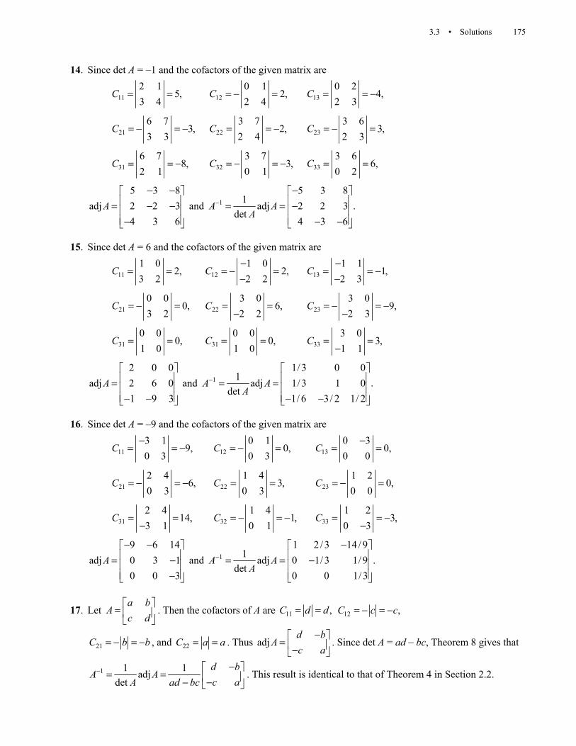
3.3 • Solutions 175
14. Since det A = –1 and the cofactors of the given matrix are
112 1
5,3 4
C = = 120 1
2,2 4
C = − = 130 2
4,2 3
C = = −
216 7
3,3 3
C = − = − 223 7
2,2 4
C = = − 233 6
3,2 3
C = − =
316 7
8,2 1
C = = − 323 7
3,0 1
C = − = − 333 6
6,0 2
C = =
5 3 8
adj 2 2 34 3 6
A− −
= − − −
and 15 3 8
1 adj 2 2 3 .det
4 3 6A A
A−
− = = − − −
15. Since det A = 6 and the cofactors of the given matrix are
111 0
2,3 2
C = = 121 0
2,2 2
C−
= − =−
131 1
1,2 3
C−
= = −−
210 0
0,3 2
C = − = 223 0
6,2 2
C = =−
233 0
9,2 3
C = − = −−
310 0
0,1 0
C = = 310 0
0,1 0
C = = 333 0
3,1 1
C = =−
2 0 0
adj 2 6 01 9 3
A = − −
and 11/ 3 0 0
1 adj 1/ 3 1 0 .det
1/ 6 3/ 2 1/ 2A A
A−
= = − −
16. Since det A = –9 and the cofactors of the given matrix are
113 1
9,0 3
C−
= = − 120 1
0,0 3
C = − = 130 3
0,0 0
C−
= =
212 4
6,0 3
C = − = − 221 4
3,0 3
C = = 231 2
0,0 0
C = − =
312 4
14,3 1
C = =−
321 4
1,0 1
C = − = − 331 2
3,0 3
C = = −−
9 6 14
adj 0 3 10 0 3
A− − = − −
and 11 2 / 3 14 / 9
1 adj 0 1/ 3 1/ 9 .det
0 0 1/ 3A A
A−
− = = −
17. Let a b
Ac d
=
. Then the cofactors of A are 11 ,C d d= = 12 ,C c c= − = −
21C b b= − = − , and 22C a a= = . Thus adjd b
Ac a
− = −
. Since det A = ad – bc, Theorem 8 gives that
1 1 1adjdet
d bA A
c aA ad bc− −
= = −− . This result is identical to that of Theorem 4 in Section 2.2.

176 CHAPTER 3 • Determinants
18. Each cofactor of A is an integer since it is a sum of products of entries in A. Hence all entries in adj A will be integers. Since det A = 1, the inverse formula in Theorem 8 shows that all the entries in 1A− will be integers.
19. The parallelogram is determined by the columns of 5 62 4
A
=
, so the area of the parallelogram is
|det A| = |8| = 8.
20. The parallelogram is determined by the columns of 1 43 5
A−
= − , so the area of the parallelogram is
|det A| = |–7| = 7.
21. First translate one vertex to the origin. For example, subtract (–1, 0) from each vertex to get a new parallelogram with vertices (0, 0),(1, 5),(2, –4), and (3, 1). This parallelogram has the same area as the
original, and is determined by the columns of 1 25 4
A
= − , so the area of the parallelogram is
|det A| = |–14| = 14.
22. First translate one vertex to the origin. For example, subtract (0, –2) from each vertex to get a new parallelogram with vertices (0, 0),(6, 1),(–3, 3), and (3, 4). This parallelogram has the same area as
the original, and is determined by the columns of 6 31 3
A−
=
, so the area of the parallelogram is
|det A| = |21| = 21.
23. The parallelepiped is determined by the columns of 1 1 70 2 12 4 0
A = −
, so the volume of the
parallelepiped is |det A| = |22| = 22.
24. The parallelepiped is determined by the columns of 1 2 14 5 20 2 1
A− −
= − −
, so the volume of the
parallelepiped is |det A| = |–15| = 15.
25. The Invertible Matrix Theorem says that a 3 × 3 matrix A is not invertible if and only if its columns are linearly dependent. This will happen if and only if one of the columns is a linear combination of the others; that is, if one of the vectors is in the plane spanned by the other two vectors. This is equivalent to the condition that the parallelepiped determined by the three vectors has zero volume, which is in turn equivalent to the condition that det A = 0.
26. By definition, p + S is the set of all vectors of the form p + v, where v is in S. Applying T to a typical vector in p + S, we have T(p + v) = T(p) + T(v). This vector is in the set denoted by T(p) + T(S). This proves that T maps the set p + S into the set T(p) + T(S).
Conversely, any vector in T(p) + T(S) has the form T(p) + T(v) for some v in S. This vector may be written as T(p + v). This shows that every vector in T(p) + T(S) is the image under T of some point p + v in p + S.

3.3 • Solutions 177
27. Since the parallelogram S is determined by the columns of 2 23 5
− −
, the area of S is
2 2det | 4 | 4.
3 5− −
= − =
The matrix A has 6 2
det 63 2
A−
= =−
. By Theorem 10, the area of T(S) is
|det A|{area of S} = 6 ⋅ 4 = 24. Alternatively, one may compute the vectors that determine the image, namely, the columns of
[ ]1 26 2 2 2 18 223 2 3 5 12 16
A− − − − −
= = − b b
The determinant of this matrix is –24, so the area of the image is 24.
28. Since the parallelogram S is determined by the columns of 4 07 1
−
, the area of S is
4 0det | 4 | 4
7 1
= = − . The matrix A has
7 2det 5
1 1A = = . By Theorem 10, the area of T(S) is
|det A|{area of S} =5 ⋅ 4 = 20. Alternatively, one may compute the vectors that determine the image, namely, the columns of
[ ]1 27 2 4 0 14 21 1 7 1 3 1
A
= = − − b b
The determinant of this matrix is 20, so the area of the image is 20.
29. The area of the triangle will be one half of the area of the parallelogram determined by 1v and 2.v By Theorem 9, the area of the triangle will be (1/2)|det A|, where [ ]1 2 .A = v v
30. Translate R to a new triangle of equal area by subtracting 3 3( , )x y from each vertex. The new triangle has vertices (0, 0), 1 3 1 3( , )x x y y− − , and 2 3 2 3( , ).x x y y− − By Exercise 29, the area of the triangle will be
1 3 2 3
1 3 2 3
1 det .2
x x x xy y y y
− − − −
Now consider using row operations and a cofactor expansion to compute the determinant in the formula:
1 1 1 3 1 3
1 3 1 32 2 2 3 2 3
2 3 2 33 3 3 3
1 0det 1 det 0 det
1 1
x y x x y yx x y y
x y x x y yx x y y
x y x y
− − − − = − − = − −
By Theorem 5,
1 3 1 3 1 3 2 3
2 3 2 3 1 3 2 3det det
x x y y x x x xx x y y y y y y
− − − − = − − − −
So the above observation allows us to state that the area of the triangle will be
1 1
1 3 2 32 2
1 3 2 33 3
11 1det det 12 2
1
x yx x x x
x yy y y y
x y
− − = − −

178 CHAPTER 3 • Determinants
31. a. To show that T(S) is bounded by the ellipsoid with equation 22 231 2
2 2 2 1xx xa b c
+ + = , let 1
2
3
uuu
=
u and let
1
2
3
xx Ax
= =
x u . Then 1 1 /u x a= , 2 2 /u x b= , and 3 3 /u x c= , and u lies inside S (or 2 2 21 2 3 1u u u+ + ≤ ) if
and only if x lies inside T(S) (or 22 231 2
2 2 2 1xx xa b c
+ + ≤ ).
b. By the generalization of Theorem 10, {volume of ellipsoid} {volume of ( )}T S=
4 4| det | {volume of }3 3
abcA S abc π π= ⋅ = =
32. a. A linear transformation T that maps S onto S ′ will map 1e to 1,v 2e to 2 ,v and 3e to 3;v that is,
1 1( )T =e v , 2 2( )T =e v , and 3 3( ) .T =e v The standard matrix for this transformation will be [ ] [ ]1 2 3 1 2 3( ) ( ) ( ) .A T T T= =e e e v v v
b. The area of the base of S is (1/2)(1)(1) = 1/2, so the volume of S is (1/3)(1/2)(1) = 1/6. By part a. T(S) = S′ , so the generalization of Theorem 10 gives that the volume of S′ is |det A|{volume of S} = (1/6)|det A|.
33. [M] Answers will vary. In MATLAB, entries in B – inv(A) are approximately 1510− or smaller.
34. [M] Answers will vary, as will the commands which produce the second entry of x. For example, the MATLAB command is x2 = det([A(:,1) b A(:,3:4)])/det(A) while the Mathematica command is x2 = Det[{Transpose[A][[1]],b,Transpose[A][[3]], Transpose[A][[4]]}]/Det[A].
35. [M] MATLAB Student Version 4.0 uses 57,771 flops for inv A and 14,269,045 flops for the inverse formula. The inv(A) command requires only about 0.4% of the operations for the inverse formula.
Chapter 3 SUPPLEMENTARY EXERCISES
1. a. True. The columns of A are linearly dependent. b. True. See Exercise 30 in Section 3.2. c. False. See Theorem 3(c); in this case 3det 5 5 detA A= .
d. False. Consider 2 00 1
A
=
, 1 00 3
B
=
, and 3 00 4
A B
+ =
.
e. False. By Theorem 6, 3 3det 2A = . f. False. See Theorem 3(b). g. True. See Theorem 3(c). h. True. See Theorem 3(a). i. False. See Theorem 5. j. False. See Theorem 3(c); this statement is false for n × n invertible matrices with n an even integer. k. True. See Theorems 6 and 5; 2det (det )TA A A= .

Chapter 3 • Supplementary Exercises 179
l. False. The coefficient matrix must be invertible. m. False. The area of the triangle is 5. n. True. See Theorem 6; 3 3det (det )A A= . o. False. See Exercise 31 in Section 3.2. p. True. See Theorem 6.
2. 12 13 14 12 13 1415 16 17 3 3 3 018 19 20 6 6 6
= =
3. 1 1 11 0 ( )( ) 0 1 1 01 0 0 1 1
a b c a b c a b cb a c b a a b b a c ac a b c a a c
+ + ++ = − − = − − − =+ − − −
4. 1 1 1 01 1 1
a b c a b c a b ca x b x c x x x x xya y b y c y y y y
+ + + = = =+ + +
5.
9 1 9 9 99 9 9 2
4 0 59 0 9 9 24 0 5 0
( 1) ( 1)( 2) 9 3 94 0 0 5 09 3 9 0
6 0 79 0 3 9 06 0 7 0
6 0 0 7 0
= − = − −
4 5
( 1)( 2)(3) ( 1)( 2)(3)( 2) 126 7
= − − = − − − = −
6.
4 8 8 8 54 8 8 5
4 8 50 1 0 0 06 8 8 7 4 5
(1) (1)(2) 6 8 7 (1)(2)( 3) (1)(2)( 3)( 2) 126 8 8 8 70 8 3 0 6 7
0 3 00 8 8 3 00 2 0 0
0 8 2 0 0
= = = − = − − =
7. Expand along the first row to obtain
1 1 1 11 1
2 2 2 22 2
11 1
1 1 0.1 1
1
x yx y y x
x y x yx y y x
x y= − + = This is an equation of the form ax + by + c = 0,
and since the points 1 1( , )x y and 2 2( , )x y are distinct, at least one of a and b is not zero. Thus the equation is the equation of a line. The points 1 1( , )x y and 2 2( , )x y are on the line, because when the coordinates of one of the points are substituted for x and y, two rows of the matrix are equal and so the determinant is zero.

180 CHAPTER 3 • Determinants
8. Expand along the first row to obtain
1 1 1 11 1 1 1
11 1
1 1 1( ) ( ) (1) 0.1 0 0 1
0 1
x yx y y x
x y x y mx y x m ym m
m= − + = − − + = This equation may be
rewritten as 1 1 0,mx y mx y− − + = or 1 1( ).y y m x x− = −
9.
2 2 2
2 2 2
2 2 2
1 1 1det 1 0 0 ( )( )
0 ( )( )1 0
a a a a a aT b b b a b a b a b a b a
c a c a c ac c c a c a
= = − − = − − +− − +− −
2 21 1( )( ) 0 1 ( )( ) 0 1 ( )( )( )
0 1 0 0
a a a ab a c a b a b a c a b a b a c a c b
c a c b= − − + = − − + = − − −
+ −
10. Expanding along the first row will show that 2 30 1 2 3( ) det .f t V c c t c t c t= = + + + By Exercise 9,
21 1
23 2 2 2 1 3 1 3 2
23 3
1
1 ( )( )( ) 0
1
x x
c x x x x x x x x
x x
= = − − − ≠
since 1x , 2x , and 3x are distinct. Thus f (t) is a cubic polynomial. The points 1( ,0)x , 2( ,0)x , and 3( ,0)x are on the graph of f, since when any of 1x , 2x or 3x are substituted for t, the matrix has two equal rows and thus its determinant (which is f (t)) is zero. Thus ( ) 0if x = for i = 1, 2, 3.
11. To tell if a quadrilateral determined by four points is a parallelogram, first translate one of the vertices to the origin. If we label the vertices of this new quadrilateral as 0, 1v , 2v , and 3v , then they will be the vertices of a parallelogram if one of 1v , 2v , or 3v is the sum of the other two. In this example, subtract (1, 4) from each vertex to get a new parallelogram with vertices 0 = (0, 0), 1 ( 2,1)= −v , 2 (2,5)=v , and
3 (4,4)=v . Since 2 3 1= +v v v , the quadrilateral is a parallelogram as stated. The translated parallelogram has the same area as the original, and is determined by the columns of
[ ]1 32 41 4
A−
= =
v v , so the area of the parallelogram is |det A| = |–12| = 12.
12. A 2 × 2 matrix A is invertible if and only if the parallelogram determined by the columns of A has nonzero area.
13. By Theorem 8, 11(adj )det
A A A A IA
−⋅ = = . By the Invertible Matrix Theorem, adj A is invertible and
1 1(adj )det
A AA
− = .
14. a. Consider the matrix kk
A OA
O I
=
, where 1 ≤ k ≤ n and O is an appropriately sized zero matrix. We
will show that det detkA A= for all 1 ≤ k ≤ n by mathematical induction.

Chapter 3 • Supplementary Exercises 181
First let k = 1. Expand along the last row to obtain ( 1) ( 1)
1det det ( 1) 1 det det .1
n nA OA A A
O+ + +
= = − ⋅ ⋅ =
Now let 1 < k ≤ n and assume that 1det det .kA A− = Expand along the last row of kA to obtain
( ) ( )1 1det det ( 1) 1 det det det .n k n k
k k kk
A OA A A A
O I+ + +
− −
= = − ⋅ ⋅ = =
Thus we have proven the result,
and the determinant of the matrix in question is det A.
b. Consider the matrix kk
k
I OA
C D
=
, where 1 ≤ k ≤ n, kC is an n × k matrix and O is an appropriately
sized zero matrix. We will show that det detkA D= for all 1 ≤ k ≤ n by mathematical induction.
First let k = 1. Expand along the first row to obtain 1 1
11
1det det ( 1) 1 det det .
OA D D
C D+
= = − ⋅ ⋅ =
Now let 1 < k ≤ n and assume that 1det det .kA D− = Expand along the first row of kA to obtain
1 11 1det det ( 1) 1 det det det .k
k k kk
I OA A A D
C D+
− −
= = − ⋅ ⋅ = =
Thus we have proven the result, and the
determinant of the matrix in question is det D. c. By combining parts a. and b., we have shown that
det det det (det )(det ).A O A O I O
A DC D O I C D
= =
From this result and Theorem 5, we have
det det det (det )(det )T T
T TT T
A B A B A OA D
O D O D B D
= = =
(det )(det ).A D=
15. a. Compute the right side of the equation:
I O A B A BX I O Y XA XB Y
= +
Set this equal to the left side of the equation:
so thatA B A B
XA C XB Y DC D XA XB Y
= = + = +
Since XA = C and A is invertible, 1.X CA−= Since XB + Y = D, 1Y D XB D CA B−= − = − . Thus by Exercise 14(c),
1 1det det detI O A BA B
C D CA I O D CA B− −
= −
1(det )(det ( ))A D CA B−= −
b. From part a.,
1 1det (det )(det ( )) det[ ( )]A B
A D CA B A D CA BC D
− − = − = −
1 1det[ ] det[ ]AD ACA B AD CAA B− −= − = − det[ ]AD CB= −

182 CHAPTER 3 • Determinants
16. a. Doing the given operations does not change the determinant of A since the given operations are all row replacement operations. The resulting matrix is
0 00 00 0 0
a b a ba b a b
a b
b b b a
− − + … − − + … − … …
b. Since column replacement operations are equivalent to row operations on TA and det detTA A= , the given operations do not change the determinant of the matrix. The resulting matrix is
0 0 00 0 00 0 0
2 3 ( 1)
a ba b
a b
b b b a n b
− … − … − … … + −
c. Since the preceding matrix is a triangular matrix with the same determinant as A,
1det ( ) ( ( 1) ).nA a b a n b−= − + −
17. First consider the case n = 2. In this case
2det ( ),det ,0
a b b b bB a a b C ab b
a b a−
= = − = = −
so 2 2 2 2 1det det det ( ) ( )( ) ( ) ( (2 1) )A B C a a b ab b a b a b a b a b a b−= + = − + − = − = − + = − + − , and the formula holds for n = 2.
Now assume that the formula holds for all (k – 1) × (k – 1) matrices, and let A, B, and C be k × k matrices. By a cofactor expansion along the first column,
2 1det ( ) ( )( ) ( ( 2) ) ( ) ( ( 2) )k k
a b bb a b
B a b a b a b a k b a b a k b
b b a
− −
……
= − = − − + − = − + −
…
since the matrix in the above formula is a (k – 1) × (k – 1) matrix. We can perform a series of row operations on C to “zero out” below the first pivot, and produce the following matrix whose determinant is det C:
0 0
.
0 0
b b ba b
a b
… − … … −
Since this is a triangular matrix, we have found that 1det ( )kC b a b −= − . Thus
1 1 1det det det ( ) ( ( 2) ) ( ) ( ) ( ( 1) ),k k kA B C a b a k b b a b a b a k b− − −= + = − + − + − = − + −
which is what was to be shown. Thus the formula has been proven by mathematical induction.
18. [M] Since the first matrix has a = 3, b = 8, and n = 4, its determinant is 4 1 3(3 8) (3 (4 1)8) ( 5) (3 24) ( 125)(27) 3375.−− + − = − + = − = − Since the second matrix has a = 8, b = 3,
and n = 5, its determinant is 5 1 4(8 3) (8 (5 1)3) (5) (8 12) (625)(20) 12,500.−− + − = + = =

Chapter 3 • Supplementary Exercises 183
19. [M] We find that
1 1 1 1 11 1 1 1
1 1 1 1 2 2 2 21 2 2 2
1 2 2 1, 1, 1.1 2 3 3 31 2 3 3
1 2 3 1 2 3 4 41 2 3 4
1 2 3 4 5
= = =
Our conjecture then is that
1 1 1 11 2 2 2
1.1 2 3 3
1 2 3 n
……
=…
…
To show this, consider using row replacement operations to “zero out” below the first pivot. The resulting matrix is
1 1 1 10 1 1 1
.0 1 2 2
0 1 2 1n
… … … … −
Now use row replacement operations to “zero out” below the second pivot, and so on. The final matrix which results from this process is
1 1 1 10 1 1 1
,0 0 1 1
0 0 0 1
… … … …
which is an upper triangular matrix with determinant 1.
20. [M] We find that
1 1 1 1 11 1 1 1
1 1 1 1 3 3 3 31 3 3 3
1 3 3 6, 18, 54.1 3 6 6 61 3 6 6
1 3 6 1 3 6 9 91 3 6 9
1 3 6 9 12
= = =
Our conjecture then is that
2
1 1 1 11 3 3 3
2 3 .1 3 6 6
1 3 6 3( 1)
n
n
−
……
= ⋅…
… −

184 CHAPTER 3 • Determinants
To show this, consider using row replacement operations to “zero out” below the first pivot. The resulting matrix is
1 1 1 10 2 2 2
.0 2 5 5
0 2 5 3( 1) 1n
… … … … − −
Now use row replacement operations to “zero out” below the second pivot. The matrix which results from this process is
1 1 1 1 1 1 10 2 2 2 2 2 20 0 3 3 3 3 3
.0 0 3 6 6 6 60 0 3 6 9 9 9
0 0 3 6 9 12 3( 2)n
… … … … … … −
This matrix has the same determinant as the original matrix, and is recognizable as a block matrix of the form
,A BO D
where
3 3 3 3 3 1 1 1 1 13 6 6 6 6 1 2 2 2 2
1 1and 3 .3 6 9 9 9 1 2 3 3 3
0 2
3 6 9 12 3( 2) 1 2 3 4 2
A D
n n
… … … … = = =… … … − − …
As in Exercise 14(c), the determinant of the matrix A BO D
is (det A)(det D) = 2 det D.
Since D is an (n – 2) × (n – 2) matrix,
2 2 2
1 1 1 1 11 2 2 2 2
det 3 3 (1) 31 2 3 3 3
1 2 3 4 2
n n nD
n
− − −
……
= = =…
… −
by Exercise 19. Thus the determinant of the matrix A BO D
is 22det 2 3 .nD −= ⋅

185
4.1 SOLUTIONS
Notes: This section is designed to avoid the standard exercises in which a student is asked to check ten axioms on an array of sets. Theorem 1 provides the main homework tool in this section for showing that a set is a subspace. Students should be taught how to check the closure axioms. The exercises in this section (and the next few sections) emphasize n, to give students time to absorb the abstract concepts. Other vectors do appear later in the chapter: the space of signals is used in Section 4.8, and the spaces n of polynomials are used in many sections of Chapters 4 and 6.
1. a. If u and v are in V, then their entries are nonnegative. Since a sum of nonnegative numbers is nonnegative, the vector u + v has nonnegative entries. Thus u + v is in V.
b. Example: If 22
=
u and c = –1, then u is in V but cu is not in V.
2. a. If xy
=
u is in W, then the vector x cx
c cy cy
= =
u is in W because 2( )( ) ( ) 0cx cy c xy= ≥
since xy ≥ 0.
b. Example: If 17
− = −
u and 23
=
v , then u and v are in W but u + v is not in W.
3. Example: If .5.5
=
u and c = 4, then u is in H but cu is not in H. Since H is not closed under scalar
multiplication, H is not a subspace of 2.
4. Note that u and v are on the line L, but u + v is not.
u
v
L
u+v
5. Yes. Since the set is 2Span{ }t , the set is a subspace by Theorem 1.

186 CHAPTER 4 • Vector Spaces
6. No. The zero vector is not in the set.
7. No. The set is not closed under multiplication by scalars which are not integers.
8. Yes. The zero vector is in the set H. If p and q are in H, then (p + q)(0) = p(0) + q(0) = 0 + 0 = 0, so p + q is in H. For any scalar c, (cp)(0) = c ⋅ p(0) = c ⋅ 0 = 0, so cp is in H. Thus H is a subspace by Theorem 1.
9. The set H = Span {v}, where 132
=
v . Thus H is a subspace of 3 by Theorem 1.
10. The set H = Span {v}, where 201
= −
v . Thus H is a subspace of 3 by Theorem 1.
11. The set W = Span {u, v}, where 510
=
u and 201
=
v . Thus W is a subspace of 3 by Theorem 1.
12. The set W = Span {u, v}, where
1120
=
u and
3114
− = −
v . Thus W is a subspace of 4 by Theorem 1.
13. a. The vector w is not in the set 1 2 3{ , , }v v v . There are 3 vectors in the set 1 2 3{ , , }.v v v
b. The set 1 2 3Span{ , , }v v v contains infinitely many vectors.
c. The vector w is in the subspace spanned by 1 2 3{ , , }v v v if and only if the equation
1 1 2 2 3 3x x x+ + =v v v w has a solution. Row reducing the augmented matrix for this system of linear equations gives
1 2 4 3 1 0 0 10 1 2 1 0 1 2 1 ,1 3 6 2 0 0 0 0
∼ −
so the equation has a solution and w is in the subspace spanned by 1 2 3{ , , }v v v .
14. The augmented matrix is found as in Exercise 13c. Since
1 2 4 8 1 0 0 00 1 2 4 0 1 2 0 ,1 3 6 7 0 0 0 1
∼ −
the equation 1 1 2 2 3 3x x x+ + =v v v w has no solution, and w is not in the subspace spanned by
1 2 3{ , , }.v v v
15. Since the zero vector is not in W, W is not a vector space.
16. Since the zero vector is not in W, W is not a vector space.

4.1 • Solutions 187
17. Since a vector w in W may be written as
1 1 00 1 11 0 10 1 0
a b c
− − = + + −
w
1 1 00 1 1
, ,1 0 10 1 0
S
− − = −
is a set that spans W.
18. Since a vector w in W may be written as
4 3 00 0 01 1 12 0 1
a b c
= + + −
w
4 3 00 0 0
, ,1 1 12 0 1
S
= −
is a set that spans W.
19. Let H be the set of all functions described by 1 2( ) cos sin .y t c t c tω ω= + Then H is a subset of the vector space V of all real-valued functions, and may be written as H = Span {cos ωt, sin ωt}. By Theorem 1, H is a subspace of V and is hence a vector space.
20. a. The following facts about continuous functions must be shown. 1. The constant function f(t) = 0 is continuous. 2. The sum of two continuous functions is continuous. 3. A constant multiple of a continuous function is continuous. b. Let H = {f in C[a, b]: f(a) = f(b)}. 1. Let g(t) = 0 for all t in [a, b]. Then g(a) = g(b) = 0, so g is in H. 2. Let g and h be in H. Then g(a) = g(b) and h(a) = h(b), and (g + h)(a) = g(a) + h(a) = g(b) + h(b) = (g + h)(b), so g + h is in H. 3. Let g be in H. Then g(a) = g(b), and (cg)(a) = cg(a) = cg(b) = (cg)(b), so cg is in H. Thus H is a subspace of C[a, b].
21. The set H is a subspace of 2 2.M × The zero matrix is in H, the sum of two upper triangular matrices is upper triangular, and a scalar multiple of an upper triangular matrix is upper triangular.
22. The set H is a subspace of 2 4.M × The 2 × 4 zero matrix 0 is in H because F0 = 0. If A and B are matrices in H, then F(A + B) = FA + FB = 0 + 0 = 0, so A + B is in H. If A is in H and c is a scalar, then F(cA) = c(FA) = c0 = 0, so cA is in H.

188 CHAPTER 4 • Vector Spaces
23. a. False. The zero vector in V is the function f whose values f(t) are zero for all t in . b. False. An arrow in three-dimensional space is an example of a vector, but not every arrow is a vector. c. False. See Exercises 1, 2, and 3 for examples of subsets which contain the zero vector but are not
subspaces. d. True. See the paragraph before Example 6. e. False. Digital signals are used. See Example 3.
24. a. True. See the definition of a vector space. b. True. See statement (3) in the box before Example 1. c. True. See the paragraph before Example 6. d. False. See Example 8. e. False. The second and third parts of the conditions are stated incorrectly. For example, part (ii) does
not state that u and v represent all possible elements of H.
25. 2, 4
26. a. 3 b. 5 c. 4
27. a. 8 b. 3 c. 5 d. 4
28. a. 4 b. 7 c. 3 d. 5 e. 4
29. Consider u + (–1)u. By Axiom 10, u + (–1)u = 1u + (–1)u. By Axiom 8, 1u + (–1)u = (1 + (–1))u = 0u. By Exercise 27, 0u = 0. Thus u + (–1)u = 0, and by Exercise 26 (–1)u = –u.
30. By Axiom 10 u = 1u. Since c is nonzero, 1 1c c− = , and 1( )c c−=u u . By Axiom 9, 1 1 1( ) ( )c c c c c− − −= =u u 0 since cu = 0. Thus 1c−= =u 0 0 by Property (2), proven in Exercise 28.
31. Any subspace H that contains u and v must also contain all scalar multiples of u and v, and hence must also contain all sums of scalar multiples of u and v. Thus H must contain all linear combinations of u and v, or Span {u, v}.
Note: Exercises 32–34 provide good practice for mathematics majors because these arguments involve simple symbol manipulation typical of mathematical proofs. Most students outside mathematics might profit more from other types of exercises.
32. Both H and K contain the zero vector of V because they are subspaces of V. Thus the zero vector of V is in H ∩ K. Let u and v be in H ∩ K. Then u and v are in H. Since H is a subspace u + v is in H. Likewise u and v are in K. Since K is a subspace u + v is in K. Thus u + v is in H ∩ K. Let u be in H ∩ K. Then u is in H. Since H is a subspace cu is in H. Likewise v is in K. Since K is a subspace cu is in K. Thus cu is in H ∩ K for any scalar c, and H ∩ K is a subspace of V.

4.1 • Solutions 189
The union of two subspaces is not in general a subspace. For an example in 2 let H be the x-axis and let K be the y-axis. Then both H and K are subspaces of 2, but H ∪ K is not closed under vector addition. The subset H ∪ K is thus not a subspace of 2.
33. a. Given subspaces H and K of a vector space V, the zero vector of V belongs to H + K, because 0 is in both H and K (since they are subspaces) and 0 = 0 + 0. Next, take two vectors in H + K, say
1 1 1= +w u v and 2 2 2= +w u v where 1u and 2u are in H, and 1v and 2v are in K. Then
1 2 1 1 2 2 1 2 1 2( ) ( )+ = + + + = + + +w w u v u v u u v v
because vector addition in V is commutative and associative. Now 1 2+u u is in H and 1 2+v v is in K because H and K are subspaces. This shows that 1 2+w w is in H + K. Thus H + K is closed under addition of vectors. Finally, for any scalar c,
1 1 1 1 1( )c c c c= + = +w u v u v
The vector 1cu belongs to H and 1cv belongs to K, because H and K are subspaces. Thus, 1cw belongs to H + K, so H + K is closed under multiplication by scalars. These arguments show that H + K satisfies all three conditions necessary to be a subspace of V.
b. Certainly H is a subset of H + K because every vector u in H may be written as u + 0, where the zero vector 0 is in K (and also in H, of course). Since H contains the zero vector of H + K, and H is closed under vector addition and multiplication by scalars (because H is a subspace of V ), H is a subspace of H + K. The same argument applies when H is replaced by K, so K is also a subspace of H + K.
34. A proof that 1 1Span{ , , , , , }p qH K+ = … …u u v v has two parts. First, one must show that H + K is a subset of 1 1Span{ , , , , , }.p q… …u u v v Second, one must show that 1 1Span{ , , , , , }p q… …u u v v is a subset of H + K. (1) A typical vector H has the form 1 1 p pc c+…+u u and a typical vector in K has the form
1 1 .q qd d+…+v v The sum of these two vectors is a linear combination of 1 1, , , , ,p q… …u u v v and so belongs to 1 1Span{ , , , , , }.p q… …u u v v Thus H + K is a subset of 1 1Span{ , , , , , }.p q… …u u v v
(2) Each of the vectors 1 1, , , , ,p q… …u u v v belongs to H + K, by Exercise 33(b), and so any linear combination of these vectors belongs to H + K, since H + K is a subspace, by Exercise 33(a). Thus,
1 1Span{ , , , , , }p q… …u u v v is a subset of H + K.
35. [M] Since
7 4 9 9 1 0 0 15/ 24 5 4 7 0 1 0 3
,2 1 4 4 0 0 1 11/ 29 7 7 8 0 0 0 0
− − − − ∼ − − − −
w is in the subspace spanned by 1 2 3{ , , }.v v v
36. [M] Since
[ ]
5 5 9 6 1 0 0 11/ 28 8 6 7 0 1 0 2
,5 9 3 1 0 0 1 7 / 23 2 7 4 0 0 0 0
A
− − − − = ∼ − − − − −
y
y is in the subspace spanned by the columns of A.

190 CHAPTER 4 • Vector Spaces
37. [M] The graph of f(t) is given below. A conjecture is that f(t) = cos 4t.
1 2 3 4 5 6
–1
–0.5
0.5
1
The graph of g(t) is given below. A conjecture is that g(t) = cos 6t.
1 2 3 4 5 6
–1
–0.5
0.5
1
38. [M] The graph of f(t) is given below. A conjecture is that f(t) = sin 3t.
1 2 3 4 5 6
–1
–0.5
0.5
1
The graph of g(t) is given below. A conjecture is that g(t) = cos 4t.
1 2 3 4 5 6
–1
–0.5
0.5
1
The graph of h(t) is given below. A conjecture is that h(t) = sin 5t.
1 2 3 4 5 6
–1
–0.5
0.5
1

4.2 • Solutions 191
4.2 SOLUTIONS
Notes: This section provides a review of Chapter 1 using the new terminology. Linear tranformations are introduced quickly since students are already comfortable with the idea from n. The key exercises are 17–26, which are straightforward but help to solidify the notions of null spaces and column spaces. Exercises 30–36 deal with the kernel and range of a linear transformation and are progressively more advanced theoretically. The idea in Exercises 7–14 is for the student to use Theorems 1, 2, or 3 to determine whether a given set is a subspace.
1. One calculates that
3 5 3 1 06 2 0 3 0 ,8 4 1 4 0
A− −
= − = − −
w
so w is in Nul A.
2. One calculates that
5 21 19 5 0
13 23 2 3 0 ,8 14 1 2 0
A = − =
w
so w is in Nul A.
3. First find the general solution of Ax = 0 in terms of the free variables. Since
[ ] 1 0 7 6 0,
0 1 4 2 0A
− ∼ −
0
the general solution is 1 3 47 6x x x= − , 2 3 44 2x x x= − + , with 3x and 4x free. So
1
23 4
3
4
7 64 2
,1 00 1
xx
x xxx
− − = = +
x
and a spanning set for Nul A is
7 64 2
, .1 00 1
− −
4. First find the general solution of Ax = 0 in terms of the free variables. Since
[ ] 1 6 0 0 0,
0 0 1 0 0A
− ∼
0
the general solution is 1 26x x= , 3 0x = , with 2x and 4x free. So
1
22 4
3
4
6 01 0
,0 00 1
xx
x xxx
= = +
x

192 CHAPTER 4 • Vector Spaces
and a spanning set for Nul A is
6 01 0
, .0 00 1
5. First find the general solution of Ax = 0 in terms of the free variables. Since
[ ]1 2 0 4 0 00 0 1 9 0 0 ,0 0 0 0 1 0
A−
∼ −
0
the general solution is 1 2 42 4x x x= − , 3 49x x= , 5 0x = , with 2x and 4x free. So
1
2
2 43
4
5
2 41 0
,0 90 10 0
xx
x xxxx
− = = +
x
and a spanning set for Nul A is
2 41 0
, .0 90 10 0
−
6. First find the general solution of Ax = 0 in terms of the free variables. Since
[ ]1 0 6 8 1 00 1 2 1 0 0 ,0 0 0 0 0 0
A−
∼ −
0
the general solution is 1 3 4 56 8x x x x= − + − , 2 3 42x x x= − , with 3x , 4x , and 5x free. So
1
2
3 4 53
4
5
6 8 12 1 0
,1 0 00 1 00 0 1
xx
x x xxxx
− − − = = + +
x
and a spanning set for Nul A is
6 8 12 1 0
, , .1 0 00 1 00 0 1
− − −

4.2 • Solutions 193
7. The set W is a subset of 3. If W were a vector space (under the standard operations in 3), then it would be a subspace of 3. But W is not a subspace of 3 since the zero vector is not in W. Thus W is not a vector space.
8. The set W is a subset of 3. If W were a vector space (under the standard operations in 3), then it would be a subspace of 3. But W is not a subspace of 3 since the zero vector is not in W. Thus W is not a vector space.
9. The set W is the set of all solutions to the homogeneous system of equations a – 2b – 4c = 0,
2a – c – 3d = 0. Thus W = Nul A, where 1 2 4 02 0 1 3
A− −
= − − . Thus W is a subspace of 4 by
Theorem 2, and is a vector space.
10. The set W is the set of all solutions to the homogeneous system of equations a + 3b – c = 0,
a + b + c – d = 0. Thus W = Nul A, where 1 3 1 01 1 1 1
A−
= − . Thus W is a subspace of 4 by
Theorem 2, and is a vector space.
11. The set W is a subset of 4. If W were a vector space (under the standard operations in 4), then it would be a subspace of 4. But W is not a subspace of 4 since the zero vector is not in W. Thus W is not a vector space.
12. The set W is a subset of 4. If W were a vector space (under the standard operations in 4), then it would be a subspace of 4. But W is not a subspace of 4 since the zero vector is not in W. Thus W is not a vector space.
13. An element w on W may be written as
1 6 1 60 1 0 11 0 1 0
cc d
d
− − = + =
w
where c and d are any real numbers. So W = Col A where 1 60 11 0
A−
=
. Thus W is a subspace of 3 by
Theorem 3, and is a vector space.
14. An element w on W may be written as
1 2 1 21 2 1 23 6 3 6
aa b
b
− − = + − = − − −
w
where a and b are any real numbers. So W = Col A where 1 21 23 6
A− = − −
. Thus W is a subspace of 3 by
Theorem 3, and is a vector space.

194 CHAPTER 4 • Vector Spaces
15. An element in this set may be written as
0 2 3 0 2 31 1 2 1 1 24 1 0 4 1 03 1 1 3 1 1
rr s t s
t
− − + + = − − − −
where r, s and t are any real numbers. So the set is Col A where
0 2 31 1 24 1 03 1 1
A
− = − −
.
16. An element in this set may be written as
1 1 0 1 1 02 1 1 2 1 10 5 4 0 5 40 0 1 0 0 1
bb c d c
d
− − + + = − −
where b, c and d are any real numbers. So the set is Col A where
1 1 02 1 10 5 40 0 1
A
− = −
.
17. The matrix A is a 4 × 2 matrix. Thus (a) Nul A is a subspace of 2, and (b) Col A is a subspace of 4.
18. The matrix A is a 4 × 3 matrix. Thus (a) Nul A is a subspace of 3, and (b) Col A is a subspace of 4.
19. The matrix A is a 2 × 5 matrix. Thus (a) Nul A is a subspace of 5, and (b) Col A is a subspace of 2.
20. The matrix A is a 1 × 5 matrix. Thus (a) Nul A is a subspace of 5, and (b) Col A is a subspace of 1 = .
21. Either column of A is a nonzero vector in Col A. To find a nonzero vector in Nul A, find the general solution of Ax = 0 in terms of the free variables. Since
[ ]
1 3 00 0 0
,0 0 00 0 0
A
− ∼
0

4.2 • Solutions 195
the general solution is 1 23x x= , with 2x free. Letting 2x be a nonzero value (say 2 1x = ) gives the nonzero vector
1
2
31
xx
= =
x
which is in Nul A.
22. Any column of A is a nonzero vector in Col A. To find a nonzero vector in Nul A, find the general solution of Ax = 0 in terms of the free variables. Since
[ ] 1 0 7 6 0,
0 1 4 2 0A
− ∼ −
0
the general solution is 1 3 47 6x x x= − , 2 3 44 2x x x= − + , with 3x and 4x free. Letting 3x and 4x be nonzero values (say 3 4 1x x= = ) gives the nonzero vector
1
2
3
4
1211
xxxx
− = =
x
which is in Nul A.
23. Consider the system with augmented matrix [ ]A w . Since
[ ] 1 2 1/ 3,
0 0 0A
− − ∼
w
the system is consistent and w is in Col A. Also, since
6 12 2 03 6 1 0
A−
= = − w
w is in Nul A.
24. Consider the system with augmented matrix [ ]A w . Since
[ ]1 0 1 1/ 20 1 1/ 2 1 ,0 0 0 0
A−
∼
w
the system is consistent and w is in Col A. Also, since
8 2 9 2 06 4 8 1 04 0 4 2 0
A− − − = = −
w
w is in Nul A.
25. a. True. See the definition before Example 1. b. False. See Theorem 2. c. True. See the remark just before Example 4. d. False. The equation Ax = b must be consistent for every b. See #7 in the table on page 226. e. True. See Figure 2. f. True. See the remark after Theorem 3.

196 CHAPTER 4 • Vector Spaces
26. a. True. See Theorem 2. b. True. See Theorem 3. c. False. See the box after Theorem 3. d. True. See the paragraph after the definition of a linear transformation. e. True. See Figure 2. f. True. See the paragraph before Example 8.
27. Let A be the coefficient matrix of the given homogeneous system of equations. Since Ax = 0 for 321
= −
x , x is in Nul A. Since Nul A is a subspace of 3, it is closed under scalar multiplication. Thus
3010 20
10
= −
x is also in Nul A, and 1 30x = , 2 20x = , 3 10x = − is also a solution to the system of
equations.
28. Let A be the coefficient matrix of the given systems of equations. Since the first system has a solution,
the constant vector 019
=
b is in Col A. Since Col A is a subspace of 3, it is closed under scalar
multiplication. Thus 0
5 545
=
b is also in Col A, and the second system of equations must thus have a
solution.
29. a. Since ,A =0 0 the zero vector is in Col A. b. Since ( ),A A A A A+ = + +x w x w x w is in Col A.
c. Since ( ) ( ),c A A c cA=x x x is in Col A.
30. Since ( )V WT =0 0 , the zero vector W0 of W is in the range of T. Let T(x) and T(w) be typical elements in the range of T. Then since ( ) ( ) ( ), ( ) ( )T T T T T+ = + +x w x w x w is in the range of T and the range of T is closed under vector addition. Let c be any scalar. Then since ( ) ( ), ( )cT T c cT=x x x is in the range of T and the range of T is closed under scalar multiplication. Hence the range of T is a subspace of W.
31. a. Let p and q be arbitary polynomials in 2, and let c be any scalar. Then
( )(0) (0) (0) (0) (0)
( ) ( ) ( )( )(1) (1) (1) (1) (1)
T T T+ +
+ = = = + = + + +
p q p q p qp q p q
p q p q p q
and
( )(0) (0)
( ) ( )( )(1) (1)c
T c c cTc
= = =
p pp p
p p
so T is a linear transformation.

4.2 • Solutions 197
b. Any quadratic polynomial q for which (0) 0=q and (1) 0=q will be in the kernel of T. The
polynomial q must then be a multiple of ( ) ( 1).t t t= −p Given any vector 1
2
xx
in 2, the polynomial
1 2 1( )x x x t= + −p has 1(0) x=p and 2(1) .x=p Thus the range of T is all of 2.
32. Any quadratic polynomial q for which (0) 0=q will be in the kernel of T. The polynomial q must then be 2.at bt= +q Thus the polynomials 1( )t t=p and 2
2 ( )t t=p span the kernel of T. If a vector is in the
range of T, it must be of the form .aa
If a vector is of this form, it is the image of the polynomial
( )t a=p in 2. Thus the range of T is : real .a
aa
33. a. For any A and B in 2 2M × and for any scalar c,
( ) ( ) ( ) ( ) ( ) ( ) ( )T T T T TT A B A B A B A B A B A A B B T A T B+ = + + + = + + + = + + + = +
and
( ) ( ) ( ) ( )T TT cA cA c A cT A= = =
so T is a linear transformation.
b. Let B be an element of 2 2M × with ,TB B= and let 12 .A B= Then
1 1 1 1 1 1( ) ( )2 2 2 2 2 2
T T TT A A A B B B B B B B= + = + = + = + =
c. Part b. showed that the range of T contains the set of all B in 2 2M × with .TB B= It must also be shown that any B in the range of T has this property. Let B be in the range of T. Then B = T(A) for some A in 2 2.M × Then ,TB A A= + and
( ) ( )T T T T T T T TB A A A A A A A A B= + = + = + = + =
so B has the property that .TB B=
d. Let a b
Ac d
=
be in the kernel of T. Then ( ) 0TT A A A= + = , so
2 0 0
2 0 0T a b a c a c b
A Ac d b d b c d
+ + = + = = +
Solving it is found that 0a d= = and c b= − . Thus the kernel of T is 0
: real .0b
bb
−
34. Let f and g be any elements in C[0, 1] and let c be any scalar. Then T(f) is the antiderivative F of f with F(0) = 0 and T(g) is the antiderivative G of g with G(0) = 0. By the rules for antidifferentiation +F G will be an antiderivative of ,+f g and ( )(0) (0) (0) 0 0 0.+ = + = + =F G F G Thus ( ) ( ) ( ).T T T+ = +f g f g Likewise cF will be an antiderivative of cf, and ( )(0) (0) 0 0.c c c= = =F F Thus ( ) ( ),T c cT=f f and T is a linear transformation. To find the kernel of T, we must find all functions f in C[0,1] with antiderivative equal to the zero function. The only function with this property is the zero function 0, so the kernel of T is {0}.

198 CHAPTER 4 • Vector Spaces
35. Since U is a subspace of V, V0 is in U. Since T is linear, ( ) .V WT =0 0 So W0 is in T(U). Let T(x) and T(y) be typical elements in T(U). Then x and y are in U, and since U is a subspace of V, +x y is also in U. Since T is linear, ( ) ( ) ( ).T T T+ = +x y x y So ( ) ( )T T+x y is in T(U), and T(U) is closed under vector addition. Let c be any scalar. Then since x is in U and U is a subspace of V, cx is in U. Since T is linear, ( ) ( )T c cT=x x and cT(x) is in T(U ). Thus T(U) is closed under scalar multiplication, and T(U) is a subspace of W.
36. Since Z is a subspace of W, W0 is in Z. Since T is linear, ( ) .V WT =0 0 So V0 is in U. Let x and y be typical elements in U. Then T(x) and T(y) are in Z, and since Z is a subspace of W, ( ) ( )T T+x y is also in Z. Since T is linear, ( ) ( ) ( ).T T T+ = +x y x y So ( )T +x y is in Z, and +x y is in U. Thus U is closed under vector addition. Let c be any scalar. Then since x is in U, T(x) is in Z. Since Z is a subspace of W, cT(x) is also in Z. Since T is linear, ( ) ( )cT T c=x x and T(cx) is in T(U). Thus cx is in U and U is closed under scalar multiplication. Hence U is a subspace of V.
37. [M] Consider the system with augmented matrix [ ].A w Since
[ ]
1 0 0 1/ 95 1/ 950 1 0 39 /19 20 /19
,0 0 1 267 / 95 172 / 950 0 0 0 0
A
− − ∼ −
w
the system is consistent and w is in Col A. Also, since
7 6 4 1 1 145 1 0 2 1 09 11 7 3 1 0
19 9 7 1 3 0
A
− − − − = = − − − − −
w
w is not in Nul A.
38. [M] Consider the system with augmented matrix [ ]A w . Since
[ ]
1 0 1 0 20 1 2 0 3
,0 0 0 1 10 0 0 0 0
A
− − − − ∼
w
the system is consistent and w is in Col A. Also, since
8 5 2 0 1 05 2 1 2 2 0
10 8 6 3 1 03 2 1 0 0 0
A
− − − − = = − − −
w
w is in Nul A.

4.2 • Solutions 199
39. [M] a. To show that 3a and 5a are in the column space of B, we can row reduce the matrices [ ]3B a and
[ ]3B a :
[ ]3
1 0 0 1/ 30 1 0 1/ 30 0 1 00 0 0 0
B
∼
a
[ ]5
1 0 0 10 / 30 1 0 26 / 30 0 1 40 0 0 0
B
− ∼ −
a
Since both these systems are consistent, 3a and 5a are in the column space of B. Notice that the same conclusions can be drawn by observing the reduced row echelon form for A:
1 0 1/ 3 0 10 / 30 1 1/ 3 0 26 / 30 0 0 1 40 0 0 0 0
A
− ∼ −
b. We find the general solution of Ax = 0 in terms of the free variables by using the reduced row echelon form of A given above: 1 3 5( 1/ 3) (10 / 3)x x x= − − , 2 3 5( 1/ 3) (26 / 3)x x x= − + , 4 54x x= with 3x and 5x free. So
1
2
3 53
4
5
1/ 3 10 / 31/ 3 26 / 3
,1 00 40 1
xx
x xxxx
− − − = = +
x
and a spanning set for Nul A is
1/ 3 10 / 31/ 3 26 / 3
, .1 00 40 1
− − −
c. The reduced row echelon form of A shows that the columns of A are linearly dependent and do not span 4. Thus by Theorem 12 in Section 1.9, T is neither one-to-one nor onto.
40. [M] Since the line lies both in 1 2Span{ , }H = v v and in 3 4Span{ , }K = v v , w can be written both as
1 1 2 2c c+v v and 3 3 4 4c c+v v . To find w we must find the cj’s which solve 1 1 2 2 3 3 4 4c c c c+ − − =v v v v 0 . Row reduction of [ ]1 2 3 4− −v v v v 0 yields
5 1 2 0 0 1 0 0 10 / 3 03 3 1 12 0 0 1 0 26 / 3 0 ,8 4 5 28 0 0 0 1 4 0
− − ∼ − −

200 CHAPTER 4 • Vector Spaces
so the vector of cj’s must be a multiple of (10/3, –26/3, 4, 1). One simple choice is (10, –26, 12, 3), which gives 1 2 3 410 26 12 3 (24, 48, 24)= − = + = − −w v v v v . Another choice for w is (1, –2, –1).
4.3 SOLUTIONS
Notes: The definition for basis is given initially for subspaces because this emphasizes that the basis elements must be in the subspace. Students often overlook this point when the definition is given for a vector space (see Exercise 25). The subsection on bases for Nul A and Col A is essential for Sections 4.5 and 4.6. The subsection on “Two Views of a Basis” is also fundamental to understanding the interplay between linearly independent sets, spanning sets, and bases. Key exercises in this section are Exercises 21–25, which help to deepen students’ understanding of these different subsets of a vector space.
1. Consider the matrix whose columns are the given set of vectors. This 3 × 3 matrix is in echelon form, and has 3 pivot positions. Thus by the Invertible Matrix Theorem, its columns are linearly independent and span 3. So the given set of vectors is a basis for 3.
2. Since the zero vector is a member of the given set of vectors, the set cannot be linearly independent and thus cannot be a basis for 3. Now consider the matrix whose columns are the given set of vectors. This 3 × 3 matrix has only 2 pivot positions. Thus by the Invertible Matrix Theorem, its columns do not span 3.
3. Consider the matrix whose columns are the given set of vectors. The reduced echelon form of this matrix is
1 3 3 1 0 9 / 20 2 5 0 1 5/ 22 4 1 0 0 0
− − ∼ − − −
so the matrix has only two pivot positions. Thus its columns do not form a basis for 3; the set of vectors is neither linearly independent nor does it span 3.
4. Consider the matrix whose columns are the given set of vectors. The reduced echelon form of this matrix is
2 1 7 1 0 02 3 5 0 1 01 2 4 0 0 1
− − − ∼
so the matrix has three pivot positions. Thus its columns form a basis for 3.
5. Since the zero vector is a member of the given set of vectors, the set cannot be linearly independent and thus cannot be a basis for 3. Now consider the matrix whose columns are the given set of vectors. The reduced echelon form of this matrix is
1 2 0 0 1 0 0 03 9 0 3 0 1 0 00 0 0 5 0 0 0 1
− − − ∼
so the matrix has a pivot in each row. Thus the given set of vectors spans 3.
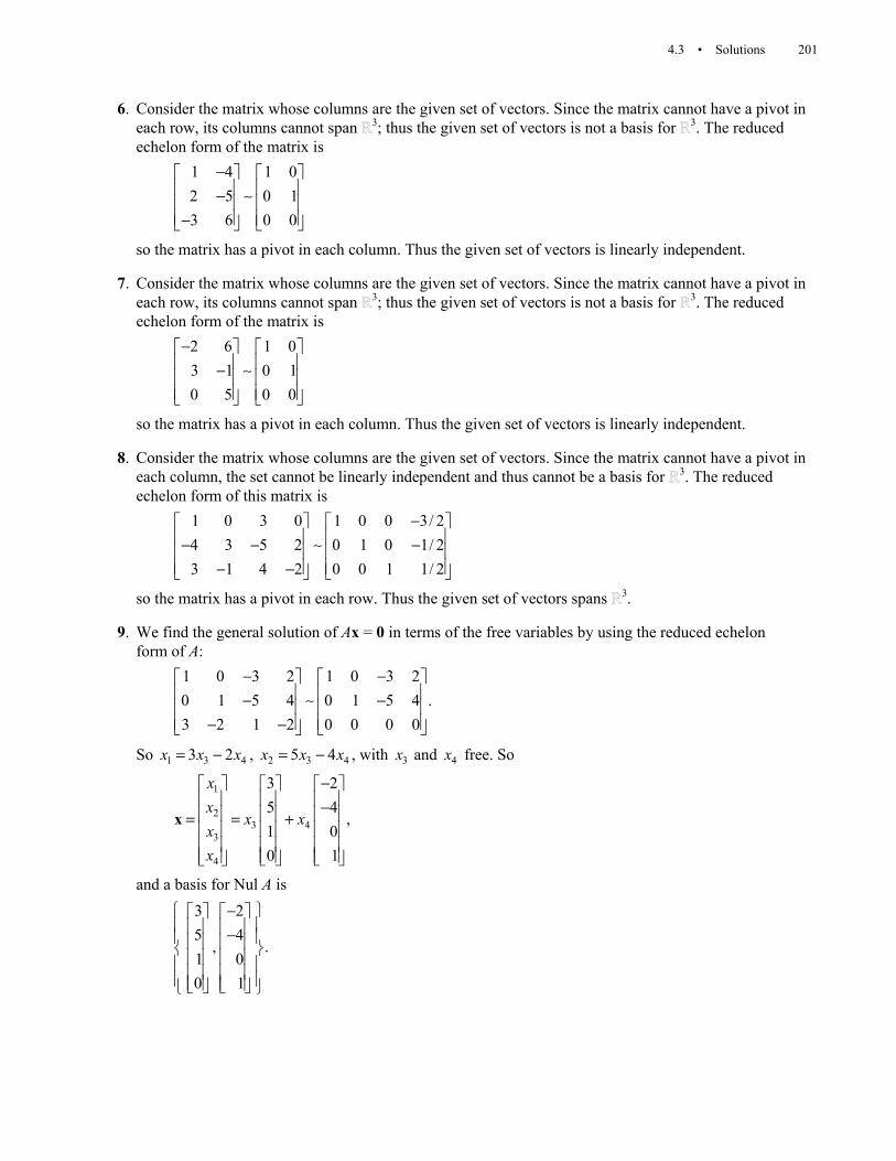
4.3 • Solutions 201
6. Consider the matrix whose columns are the given set of vectors. Since the matrix cannot have a pivot in each row, its columns cannot span 3; thus the given set of vectors is not a basis for 3. The reduced echelon form of the matrix is
1 4 1 02 5 0 13 6 0 0
− − ∼ −
so the matrix has a pivot in each column. Thus the given set of vectors is linearly independent.
7. Consider the matrix whose columns are the given set of vectors. Since the matrix cannot have a pivot in each row, its columns cannot span 3; thus the given set of vectors is not a basis for 3. The reduced echelon form of the matrix is
2 6 1 03 1 0 10 5 0 0
− − ∼
so the matrix has a pivot in each column. Thus the given set of vectors is linearly independent.
8. Consider the matrix whose columns are the given set of vectors. Since the matrix cannot have a pivot in each column, the set cannot be linearly independent and thus cannot be a basis for 3. The reduced echelon form of this matrix is
1 0 3 0 1 0 0 3/ 24 3 5 2 0 1 0 1/ 23 1 4 2 0 0 1 1/ 2
− − − ∼ − − −
so the matrix has a pivot in each row. Thus the given set of vectors spans 3.
9. We find the general solution of Ax = 0 in terms of the free variables by using the reduced echelon form of A:
1 0 3 2 1 0 3 20 1 5 4 0 1 5 4 .3 2 1 2 0 0 0 0
− − − ∼ − − −
So 1 3 43 2x x x= − , 2 3 45 4x x x= − , with 3x and 4x free. So
1
23 4
3
4
3 25 4
,1 00 1
xx
x xxx
− − = = +
x
and a basis for Nul A is
3 25 4
, .1 00 1
− −

202 CHAPTER 4 • Vector Spaces
10. We find the general solution of Ax = 0 in terms of the free variables by using the reduced echelon form of A:
1 0 5 1 4 1 0 5 0 72 1 6 2 2 0 1 4 0 6 .0 2 8 1 9 0 0 0 1 3
− − − − − ∼ − − −
So 1 3 55 7x x x= − , 2 3 54 6x x x= − , 4 53x x= , with 3x and 5x free. So
1
2
3 53
4
5
5 74 6
,1 00 30 1
xx
x xxxx
− − = = +
x
and a basis for Nul A is
5 74 6
, .1 00 30 1
− −
11. Let [ ]1 2 1A = . Then we wish to find a basis for Nul A. We find the general solution of Ax = 0 in terms of the free variables: x = –2y – z with y and z free. So
2 11 0 ,0 1
xy y zz
− − = = +
x
and a basis for Nul A is
2 11 , 0 .0 1
− −
12. We want to find a basis for the set of vectors in 2 in the line 5x – y = 0. Let [ ]5 1A = − . Then we wish to find a basis for Nul A. We find the general solution of Ax = 0 in terms of the free variables: y = 5x with x free. So
1
,5
xx
y
= =
x
and a basis for Nul A is
1
.5

4.3 • Solutions 203
13. Since B is a row echelon form of A, we see that the first and second columns of A are its pivot columns. Thus a basis for Col A is
2 42 , 6 .3 8
− − −
To find a basis for Nul A, we find the general solution of Ax = 0 in terms of the free variables: 1 3 46 5 ,x x x= − − 2 3 4( 5 / 2) (3/ 2) ,x x x= − − with 3x and 4x free. So
1
23 4
3
4
6 55/ 2 3/ 2
,1 00 1
xx
x xxx
− − − − = = +
x
and a basis for Nul A is
6 55/ 2 3/ 2
, .1 00 1
− − − −
14. Since B is a row echelon form of A, we see that the first, third, and fifth columns of A are its pivot columns. Thus a basis for Col A is
1 5 32 5 2
, , .1 0 53 5 2
− − − − −
To find a basis for Nul A, we find the general solution of Ax = 0 in terms of the free variables, mentally completing the row reduction of B to get: 1 2 42 4 ,x x x= − − 3 4(7 / 5) ,x x= 5 0,x = with 2x and 4x free. So
1
2
2 43
4
5
2 41 0
,0 7 / 50 10 0
xx
x xxxx
− − = = +
x
and a basis for Nul A is
2 41 0
, .0 7 / 50 10 0
− −

204 CHAPTER 4 • Vector Spaces
15. This problem is equivalent to finding a basis for Col A, where [ ]1 2 3 4 5A = v v v v v . Since the reduced echelon form of A is
1 0 3 1 2 1 0 3 0 40 1 4 3 1 0 1 4 0 5
,3 2 1 8 6 0 0 0 1 22 3 6 7 9 0 0 0 0 0
− − − − − − ∼ − − − − −
we see that the first, second, and fourth columns of A are its pivot columns. Thus a basis for the space spanned by the given vectors is
1 0 10 1 3
, , .3 2 82 3 7
− − − −
16. This problem is equivalent to finding a basis for Col A, where [ ]1 2 3 4 5A = v v v v v . Since the reduced echelon form of A is
1 2 6 5 0 1 0 0 1 20 1 1 3 3 0 1 0 3 5
,0 1 2 3 1 0 0 1 0 21 1 1 4 1 0 0 0 0 0
− − − − − − ∼ − − − −
we see that the first, second, and third columns of A are its pivot columns. Thus a basis for the space spanned by the given vectors is
1 2 60 1 1
, , .0 1 21 1 1
− − − −
17. [M] This problem is equivalent to finding a basis for Col A, where [ ]1 2 3 4 5A = v v v v v . Since the reduced echelon form of A is
8 4 1 6 1 1 0 0 1/ 2 39 5 4 8 4 0 1 0 5/ 2 7
,3 1 9 4 11 0 0 1 0 36 4 6 7 8 0 0 0 0 00 4 7 10 7 0 0 0 0 0
− − − − − ∼− − − − − − − − −
we see that the first, second, and third columns of A are its pivot columns. Thus a basis for the space spanned by the given vectors is
8 4 19 5 4
, , .3 1 96 4 60 4 7
− − − − − − −

4.3 • Solutions 205
18. [M] This problem is equivalent to finding a basis for Col A, where [ ]1 2 3 4 5 .A = v v v v v Since the reduced echelon form of A is
8 8 8 1 9 1 0 5/ 3 0 4 / 37 7 7 4 3 0 1 2 / 3 0 1/ 3
,6 9 4 9 4 0 0 0 1 15 5 5 6 1 0 0 0 0 07 7 7 7 0 0 0 0 0 0
− − − − ∼− − − − − − − −
we see that the first, second, and fourth columns of A are its pivot columns. Thus a basis for the space spanned by the given vectors is
8 8 17 7 4
, , .6 9 95 5 67 7 7
− − − − − −
19. Since 1 2 34 5 3 ,+ − =v v v 0 we see that each of the vectors is a linear combination of the others. Thus the sets 1 2{ , },v v 1 3{ , },v v and 2 3{ , }v v all span H. Since we may confirm that none of the three vectors is a multiple of any of the others, the sets 1 2{ , },v v 1 3{ , },v v and 2 3{ , }v v are linearly independent and thus each forms a basis for H.
20. Since 1 2 33 5 ,− + =v v v 0 we see that each of the vectors is a linear combination of the others. Thus the sets 1 2{ , },v v 1 3{ , },v v and 2 3{ , }v v all span H. Since we may confirm that none of the three vectors is a multiple of any of the others, the sets 1 2{ , },v v 1 3{ , },v v and 2 3{ , }v v are linearly independent and thus each forms a basis for H.
21. a. False. The zero vector by itself is linearly dependent. See the paragraph preceding Theorem 4. b. False. The set 1{ , , }p…b b must also be linearly independent. See the definition of a basis.
c. True. See Example 3. d. False. See the subsection “Two Views of a Basis.” e. False. See the box before Example 9.
22. a. False. The subspace spanned by the set must also coincide with H. See the definition of a basis. b. True. Apply the Spanning Set Theorem to V instead of H. The space V is nonzero because the
spanning set uses nonzero vectors. c. True. See the subsection “Two Views of a Basis.” d. False. See the two paragraphs before Example 8. e. False. See the warning after Theorem 6.
23. Let [ ]1 2 3 4 .A = v v v v Then A is square and its columns span 4 since 41 2 3 4Span{ , , , }.= v v v v
So its columns are linearly independent by the Invertible Matrix Theorem, and 1 2 3 4{ , , , }v v v v is a basis for 4.
24. Let [ ]1 .nA = …v v Then A is square and its columns are linearly independent, so its columns span n by the Invertible Matrix Theorem. Thus 1{ , , }n…v v is a basis for n.

206 CHAPTER 4 • Vector Spaces
25. In order for the set to be a basis for H, 1 2 3{ , , }v v v must be a spanning set for H; that is,
1 2 3Span{ , , }.H = v v v The exercise shows that H is a subset of 1 2 3Span{ , , }.v v v but there are vectors in
1 2 3Span{ , , }v v v which are not in H ( 1v and 3,v for example). So 1 2 3Span{ , , },H ≠ v v v and 1 2 3{ , , }v v v is not a basis for H.
26. Since sin t cos t = (1/2) sin 2t, the set {sin t, sin 2t} spans the subspace. By inspection we note that this set is linearly independent, so {sin t, sin 2t} is a basis for the subspace.
27. The set {cos ωt, sin ωt} spans the subspace. By inspection we note that this set is linearly independent, so {cos ωt, sin ωt} is a basis for the subspace.
28. The set { , }bt bte te− − spans the subspace. By inspection we note that this set is linearly independent, so
{ , }bt bte te− − is a basis for the subspace.
29. Let A be the n × k matrix [ ]1 k…v v . Since A has fewer columns than rows, there cannot be a pivot position in each row of A. By Theorem 4 in Section 1.4, the columns of A do not span n and thus are not a basis for n.
30. Let A be the n × k matrix [ ]1 k…v v . Since A has fewer rows than columns rows, there cannot be a pivot position in each column of A. By Theorem 8 in Section 1.6, the columns of A are not linearly independent and thus are not a basis for n.
31. Suppose that 1{ , , }p…v v is linearly dependent. Then there exist scalars 1, , pc c… not all zero with
1 1 .p pc c+…+ =v v 0
Since T is linear, 1 1 1 1( ) ( ) ( )p p p pT c c c T c T+…+ = +…+v v v v
and 1 1( ) ( ) .p pT c c T+…+ = =v v 0 0
Thus 1 1( ) ( )p pc T c T+…+ =v v 0
and since not all of the ic are zero, 1{ ( ), , ( )}pT T…v v is linearly dependent.
32. Suppose that 1{ ( ), , ( )}pT T…v v is linearly dependent. Then there exist scalars 1, , pc c… not all zero with
1 1( ) ( ) .p pc T c T+…+ =v v 0
Since T is linear, 1 1 1 1( ) ( ) ( ) ( )p p p pT c c c T c T T+…+ = +…+ = =v v v v 0 0
Since T is one-to-one 1 1( ) ( )p pT c c T+…+ =v v 0
implies that 1 1 .p pc c+…+ =v v 0
Since not all of the ic are zero, 1{ , , }p…v v is linearly dependent.

4.3 • Solutions 207
33. Neither polynomial is a multiple of the other polynomial. So 1 2{ , }p p is a linearly independent set in 3. Note: 1 2{ , }p p is also a linearly independent set in 2 since 1p and 2p both happen to be in 2.
34. By inspection, 3 1 2= +p p p , or 1 2 3+ − =p p p 0 . By the Spanning Set Theorem,
1 2 3 1 2Span{ , , } Span{ , }=p p p p p . Since neither 1p nor 2p is a multiple of the other, they are linearly independent and hence 1 2{ , }p p is a basis for 1 2 3Span{ , , }.p p p
35. Let 1 3{ , }v v be any linearly independent set in a vector space V, and let 2v and 4v each be linear combinations of 1v and 3.v For instance, let 2 15=v v and 4 1 3.= +v v v Then 1 3{ , }v v is a basis for
1 2 3 4Span{ , , , }.v v v v
36. [M] Row reduce the following matrices to identify their pivot columns:
[ ]1 2 3
1 0 2 1 0 22 2 2 0 1 1
,3 1 7 0 0 01 1 3 0 0 0
− = ∼ − − −
u u u so 1 2{ , }u u is a basis for H.
[ ]1 2 3
1 2 1 1 0 30 2 4 0 1 2
,8 9 6 0 0 04 5 2 0 0 0
− − − = ∼ − − −
v v v so 1 2{ , }v v is a basis for K.
[ ]1 2 3 1 2 3
1 0 2 1 2 12 2 2 0 2 43 1 7 8 9 61 1 3 4 5 2
− − = − − − − − −
u u u v v v
1 0 2 0 2 40 1 1 0 3 6
,0 0 0 1 0 30 0 0 0 0 0
− − − ∼
so 1 2 1{ , , }u u v is a basis for H + K.
37. [M] For example, writing 1 2 3 4sin cos 2 sin cos 0c t c t c t c t t⋅ + ⋅ + + =
with t = 0, .1, .2, .3 gives the following coefficent matrix A for the homogeneous system Ac = 0 (to four decimal places):
0 sin 0 cos 0 sin 0 cos 0 0 0 1 0.1 sin .1 cos .2 sin .1cos .1 .1 .0998 .9801 .0993
..2 sin .2 cos .4 sin .2 cos .2 .2 .1987 .9211 .1947.3 sin .3 cos .6 sin .3 cos .3 .3 .2955 .8253 .2823
A
= =
This matrix is invertible, so the system Ac = 0 has only the trivial solution and {t, sin t, cos 2t, sin t cos t} is a linearly independent set of functions.

208 CHAPTER 4 • Vector Spaces
38. [M] For example, writing
2 3 4 5 61 2 3 4 5 6 71 cos cos cos cos cos cos 0c c t c t c t c t c t c t⋅ + ⋅ + ⋅ + ⋅ + ⋅ + ⋅ + ⋅ =
with t = 0, .1, .2, .3, .4, .5, .6 gives the following coefficent matrix A for the homogeneous system Ac = 0 (to four decimal places):
2 3 4 5 6
2 3 4 5 6
2 3 4 5 6
2 3 4 5 6
2 3 4 5 6
2 3 4
1 cos0 cos 0 cos 0 cos 0 cos 0 cos 0
1 cos.1 cos .1 cos .1 cos .1 cos .1 cos .1
1 cos.2 cos .2 cos .2 cos .2 cos .2 cos .2
1 cos.3 cos .3 cos .3 cos .3 cos .3 cos .3
1 cos.4 cos .4 cos .4 cos .4 cos .4 cos .4
1 cos.5 cos .5 cos .5 cos .5
A =
5 6
2 3 4 5 6
cos .5 cos .5
1 cos.6 cos .6 cos .6 cos .6 cos .6 cos .6
1 1 1 1 1 1 11 .9950 .9900 .9851 .9802 .9753 .97041 .9801 .9605 .9414 .9226 .9042 .88621 .9553 .9127 .8719 .8330 .7958 .76021 .9211 .8484 .7814 .7197 .6629 .61061 .8776 .7702 .6759 .5931 .5205 .45681 .8253 .6812 .5622 .4640 .3830 .3161
=
This matrix is invertible, so the system Ac = 0 has only the trivial solution and {1, cos t, cos2t, cos3t, cos4t, cos5t, cos6t} is a linearly independent set of functions.
4.4 SOLUTIONS
Notes: Section 4.7 depends heavily on this section, as does Section 5.4. It is possible to cover the n parts of the two later sections, however, if the first half of Section 4.4 (and perhaps Example 7) is covered. The linearity of the coordinate mapping is used in Section 5.4 to find the matrix of a transformation relative to two bases. The change-of-coordinates matrix appears in Section 5.4, Theorem 8 and Exercise 27. The concept of an isomorphism is needed in the proof of Theorem 17 in Section 4.8. Exercise 25 is used in Section 4.7 to show that the change-of-coordinates matrix is invertible.
1. We calculate that
3 4 3
5 3 .5 6 7
− = + = − −
x
2. We calculate that
4 6 2
8 ( 5) .5 7 5
= + − =
x
3. We calculate that
1 5 4 1
3 4 0 2 ( 1) 7 5 .3 2 0 9
− = − + + − − = − −
x

4.4 • Solutions 209
4. We calculate that
1 3 4 0
( 4) 2 8 5 ( 7) 7 1 .0 2 3 5
− = − + − + − − = −
x
5. The matrix [ ]1 2b b x row reduces to 1 0 8
,0 1 5 −
so 8
[ ] .5B
= −
x
6. The matrix [ ]1 2b b x row reduces to 1 0 6
,0 1 2
−
so 6
[ ] .2B
− =
x
7. The matrix [ ]1 2 3b b b x row reduces to 1 0 0 10 1 0 1 ,0 0 1 3
− −
so 1
[ ] 1 .3
B
− = −
x
8. The matrix [ ]1 2 3b b b x row reduces to 1 0 0 20 1 0 0 ,0 0 1 5
−
so 2
[ ] 0 .5
B
− =
x
9. The change-of-coordinates matrix from B to the standard basis in 2 is
[ ]1 22 1
.9 8BP
= = −
b b
10. The change-of-coordinates matrix from B to the standard basis in 3 is
[ ]1 2 3
3 2 81 0 2 .4 5 7
BP = = − − −
b b b
11. Since 1BP − converts x into its B-coordinate vector, we find that
1
1 3 4 2 3 2 2 6[ ] .
5 6 6 5/ 2 3/ 2 6 4B BP−
− − − − = = = = − − − − −
x x
12. Since 1BP − converts x into its B-coordinate vector, we find that
1
1 4 6 2 7 / 2 3 2 7[ ] .
5 7 0 5/ 2 2 0 5B BP−
− − − = = = = −
x x
13. We must find 1c , 2c , and 3c such that
2 2 2 21 2 3(1 ) ( ) (1 2 ) ( ) 1 4 7 .c t c t t c t t t t t+ + + + + + = = + +p
Equating the coefficients of the two polynomials produces the system of equations
1 3
2 3
1 2 3
12 4
7
c cc c
c c c
+ =+ =
+ + =

210 CHAPTER 4 • Vector Spaces
We row reduce the augmented matrix for the system of equations to find
1 0 1 1 1 0 0 2 20 1 2 4 0 1 0 6 , so [ ] 6 .1 1 1 7 0 0 1 1 1
B
∼ = − −
p
One may also solve this problem using the coordinate vectors of the given polynomials relative to the standard basis 2{1, , };t t the same system of linear equations results.
14. We must find 1c , 2c , and 3c such that
2 2 2 21 2 3(1 ) ( ) (2 2 ) ( ) 3 6 .c t c t t c t t t t t− + − + − + = = + −p
Equating the coefficients of the two polynomials produces the system of equations
1 3
2 3
1 2 3
2 32 1
6
c cc c
c c c
+ =− =
− − + = −
We row reduce the augmented matrix for the system of equations to find
1 0 2 3 1 0 0 7 70 1 2 1 0 1 0 3 , so [ ] 3 .1 1 1 6 0 0 1 2 2
B
− ∼ − = − − − − − −
p
One may also solve this problem using the coordinate vectors of the given polynomials relative to the standard basis 2{1, , };t t the same system of linear equations results.
15. a. True. See the definition of the B-coordinate vector. b. False. See Equation (4). c. False. 3 is isomorphic to 4. See Example 5.
16. a. True. See Example 2. b. False. By definition, the coordinate mapping goes in the opposite direction. c. True. If the plane passes through the origin, as in Example 7, the plane is isomorphic to 2.
17. We must solve the vector equation 1 2 31 2 3 13 8 7 1
x x x−
+ + = − − . We row reduce the augmented
matrix for the system of equations to find
1 2 3 1 1 0 5 5
.3 8 7 1 0 1 1 2
− − ∼ − − −
Thus we can let 1 35 5x x= + and 2 32x x= − − , where 3x can be any real number. Letting 3 0x = and
3 1x = produces two different ways to express 11
as a linear combination of the other vectors:
1 25 2−v v and 2 310 3− +1v v v . There are infintely many correct answers to this problem.
18. For each k, 10 1 0k k n= ⋅ + ⋅ ⋅ ⋅ + ⋅ + ⋅ ⋅ ⋅ + ⋅b b b b , so [ ] (0, ,1, ,0) .k B k= … … =b e
19. The set S spans V because every x in V has a representation as a (unique) linear combination of elements in S. To show linear independence, suppose that 1{ , , }nS = …v v and that 1 1 n nc c+ ⋅ ⋅ ⋅ + =v v 0 for some scalars 1c , …, .nc The case when 1 0nc c= ⋅⋅ ⋅ = = is one possibility. By hypothesis, this is the unique

4.4 • Solutions 211
(and thus the only) possible representation of the zero vector as a linear combination of the elements in S. So S is linearly independent and is thus a basis for V.
20. For w in V there exist scalars 1k , 2k , 3k , and 4k such that
1 1 2 2 3 3 4 4k k k k= + + +w v v v v (1)
because 1 2 3 4{ , , , }v v v v spans V. Because the set is linearly dependent, there exist scalars 1c , 2c , 3c , and
4c not all zero, such that
1 1 2 2 3 3 4 4c c c c= + + +0 v v v v (2)
Adding (1) and (2) gives 1 1 1 2 2 2 3 3 3 4 4 4( ) ( ) ( ) ( )k c k c k c k c= + = + + + + + + +w w 0 v v v v (3)
At least one of the weights in (3) differs from the corresponding weight in (1) because at least one of the ic is nonzero. So w is expressed in more than one way as a linear combination of 1v , 2v , 3v , and 4.v
21. The matrix of the transformation will be 1
1 1 2 9 24 9 4 1BP
−− −
= = − .
22. The matrix of the transformation will be [ ] 111 .B nP −− = ⋅ ⋅ ⋅b b
23. Suppose that
[ ] [ ]B B
n
c
c
1 = = .
u w
By definition of coordinate vectors, 1 1 .n nc c= = + ⋅ ⋅ ⋅ +u w b b
Since u and w were arbitrary elements of V, the coordinate mapping is one-to-one.
24. Given 1( , , )ny y= …y in n, let 1 1 n ny y= + ⋅⋅ ⋅ +u b b . Then, by definition, [ ]B =u y . Since y was arbitrary, the coordinate mapping is onto n.
25. Since the coordinate mapping is one-to-one, the following equations have the same solutions 1, , pc c… :
1 1 p pc c+ ⋅ ⋅ ⋅ + =u u 0 (the zero vector in V ) (4)
[ ]1 1 p p BBc c + ⋅⋅ ⋅ + = u u 0 (the zero vector in n) (5)
Since the coordinate mapping is linear, (5) is equivalent to
1 1
0[ ] [ ]
0B p p Bc c
+ ⋅ ⋅ ⋅ + =
u u (6)
Thus (4) has only the trivial solution if and only if (6) has only the trivial solution. It follows that 1{ , , }p…u u is linearly independent if and only if 1{[ ] , ,[ ] }B p B…u u is linearly independent. This result
also follows directly from Exercises 31 and 32 in Section 4.3.

212 CHAPTER 4 • Vector Spaces
26. By definition, w is a linear combination of 1, , p…u u if and only if there exist scalars 1, , pc c… such that
1 1 p pc c= + ⋅ ⋅ ⋅ +w u u (7)
Since the coordinate mapping is linear, 1 1[ ] [ ] [ ]B B p p Bc c= + ⋅ ⋅ ⋅ +w u u (8)
Conversely, (8) implies (7) because the coordinate mapping is one-to-one. Thus w is a linear combination of 1, , p…u u if and only if [ ]Bw is a linear combination of 1[ ] , ,[ ] .p…u u
Note: Students need to be urged to write not just to compute in Exercises 27–34. The language in the Study Guide solution of Exercise 31 provides a model for the students. In Exercise 32, students may have difficulty distinguishing between the two isomorphic vector spaces, sometimes giving a vector in 3 as an answer for part (b).
27. The coordinate mapping produces the coordinate vectors (1, 0, 0, 1), (3, 1, –2, 0), and (0, –1, 3, –1) respectively. We test for linear independence of these vectors by writing them as columns of a matrix and row reducing:
1 3 0 1 0 00 1 1 0 1 0
.0 2 3 0 0 11 0 1 0 0 0
− ∼ − −
Since the matrix has a pivot in each column, its columns (and thus the given polynomials) are linearly independent.
28. The coordinate mapping produces the coordinate vectors (1, 0, –2, –3), (0, 1, 0, 1), and (1, 3, –2, 0) respectively. We test for linear independence of these vectors by writing them as columns of a matrix and row reducing:
1 0 1 1 0 10 1 3 0 1 3
.2 0 2 0 0 03 1 0 0 0 0
∼ − − −
Since the matrix does not have a pivot in each column, its columns (and thus the given polynomials) are linearly dependent.
29. The coordinate mapping produces the coordinate vectors (1, –2, 1, 0), (–2, 0, 0, 1), and (–8, 12, –6, 1) respectively. We test for linear independence of these vectors by writing them as columns of a matrix and row reducing:
1 2 8 1 0 62 0 12 0 1 1
.1 0 6 0 0 00 1 1 0 0 0
− − − − ∼ −
Since the matrix does not have a pivot in each column, its columns (and thus the given polynomials) are linearly dependent.

4.4 • Solutions 213
30. The coordinate mapping produces the coordinate vectors (1, –3, 3, –1), (4, –12, 9, 0), and (0, 0, 3, –4) respectively. We test for linear independence of these vectors by writing them as columns of a matrix and row reducing:
1 4 0 1 0 43 12 0 0 1 1
.3 9 3 0 0 01 0 4 0 0 0
− − − ∼ − −
Since the matrix does not have a pivot in each column, its columns (and thus the given polynomials) are linearly dependent.
31. In each part, place the coordinate vectors of the polynomials into the columns of a matrix and reduce the matrix to echelon form.
a. 1 3 4 1 1 3 4 13 5 5 0 0 4 7 35 7 6 1 0 0 0 0
− − − − − ∼ − − − − −
Since there is not a pivot in each row, the original four column vectors do not span 3. By the isomorphism between 3 and 2, the given set of polynomials does not span 2.
b. 0 1 3 2 1 2 2 05 8 4 3 0 2 6 31 2 2 0 0 0 0 7 / 2
− − − − ∼ − − −
Since there is a pivot in each row, the original four column vectors span 3. By the isomorphism between 3 and 2, the given set of polynomials spans 2.
32. a. Place the coordinate vectors of the polynomials into the columns of a matrix and reduce the matrix to
echelon form: 1 2 1 1 2 10 1 2 0 1 21 3 4 0 0 3
− ∼ − − −
The resulting matrix is invertible since it row equivalent to 3.I The original three column vectors form a basis for 3 by the Invertible Matrix Theorem. By the isomorphism between 3 and 2, the corresponding polynomials form a basis for 2.
b. Since [ ] ( 3, 1, 2),B = −q 1 2 33 2 .= − + +q p p p One might do the algebra in 2 or choose to compute 1 2 1 3 10 1 2 1 3 .1 3 4 2 8
− − = − −
This combination of the columns of the matrix corresponds to the same
combination of 1,p 2 ,p and 3.p So 2( ) 1 3 8 .t t t= + −q
33. The coordinate mapping produces the coordinate vectors (3, 7, 0, 0), (5, 1, 0, –2), (0, 1, –2, 0) and (1, 16, –6, 2) respectively. To determine whether the set of polynomials is a basis for 3, we investigate whether the coordinate vectors form a basis for 4. Writing the vectors as the columns of a matrix and row reducing
3 5 0 1 1 0 0 27 1 1 16 0 1 0 1
,0 0 2 6 0 0 1 30 2 0 2 0 0 0 0
− ∼ − − −

214 CHAPTER 4 • Vector Spaces
we find that the matrix is not row equivalent to 4.I Thus the coordinate vectors do not form a basis for 4. By the isomorphism between 4 and 3, the given set of polynomials does not form a basis for 3.
34. The coordinate mapping produces the coordinate vectors (5, –3, 4, 2), (9, 1, 8, –6), (6, –2, 5, 0), and (0, 0, 0, 1) respectively. To determine whether the set of polynomials is a basis for 3, we investigate whether the coordinate vectors form a basis for 4. Writing the vectors as the columns of a matrix, and row reducing
5 9 6 0 1 0 3/ 4 03 1 2 0 0 1 1/ 4 04 8 5 0 0 0 0 12 6 0 1 0 0 0 0
− − ∼ −
we find that the matrix is not row equivalent to I4. Thus the coordinate vectors do not form a basis for 4. By the isomorphism between 4 and 3, the given set of polynomials does not form a basis for 3.
35. To show that x is in 1 2Span{ , },H = v v we must show that the vector equation 1 1 2 2x x+ =v v x has a solution. The augmented matrix [ ]1 2v v x may be row reduced to show
11 14 19 1 0 5/ 35 8 13 0 1 8/ 3
.10 13 18 0 0 07 10 15 0 0 0
− − − − ∼
Since this system has a solution, x is in H. The solution allows us to find the B-coordinate vector for x:
since 1 1 2 2 1 2( 5 / 3) (8 / 3)x x= + = − +x v v v v , 5 / 3
[ ]8 / 3B
− =
x .
36. To show that x is in 1 2 3Span{ , , }H = v v v , we must show that the vector equation 1 1 2 2 3 3x x x+ + =v v v x has a solution. The augmented matrix [ ]1 2 3v v v x may be row reduced to show
6 8 9 4 1 0 0 34 3 5 7 0 1 0 5
.9 7 8 8 0 0 1 24 3 3 3 0 0 0 0
− − − ∼ − − − −
The first three columns show that B is a basis for H. Moreover, since this system has a solution, x is in H. The solution allows us to find the B-coordinate vector for x: since
1 1 2 2 3 3 1 2 33 5 2x x x= + + = + +x v v v v v v , 3
[ ] 5 .2
B
=
x
37. We are given that 1/ 2
[ ] 1/ 4 ,1/ 6
B
=
x where 2.6 0 01.5 , 3 , 0 .
0 0 4.8B
= −
To find the coordinates of x relative
to the standard basis in 3, we must find x. We compute that
2.6 0 0 1/ 2 1.3
[ ] 1.5 3 0 1/ 4 0 .0 0 4.8 1/ 6 0.8
B BP = = − =
x x
4.5 • Solutions 215
38. We are given that 1/ 2
[ ] 1/ 2 ,1/ 3
B
=
x where 2.6 0 01.5 , 3 , 0 .
0 0 4.8B
= −
To find the coordinates of x relative
to the standard basis in 3, we must find x. We compute that
2.6 0 0 1/ 2 1.3
[ ] 1.5 3 0 1/ 2 0.75 .0 0 4.8 1/ 3 1.6
B BP = = − =
x x
4.5 SOLUTIONS
Notes: Theorem 9 is true because a vector space isomorphic to n has the same algebraic properties as n; a proof of this result may not be needed to convince the class. The proof of Theorem 9 relies upon the fact that the coordinate mapping is a linear transformation (which is Theorem 8 in Section 4.4). If you have skipped this result, you can prove Theorem 9 as is done in Introduction to Linear Algebra by Serge Lang (Springer-Verlag, New York, 1986). There are two separate groups of true-false questions in this section; the second batch is more theoretical in nature. Example 4 is useful to get students to visualize subspaces of different dimensions, and to see the relationships between subspaces of different dimensions. Exercises 31 and 32 investigate the relationship between the dimensions of the domain and the range of a linear transformation; Exercise 32 is mentioned in the proof of Theorem 17 in Section 4.8.
1. This subspace is 1 2Span{ , },H = v v where 1
110
=
v and 2
21 .3
− =
v Since 1v and 2v are not multiples
of each other, 1 2{ , }v v is linearly independent and is thus a basis for H. Hence the dimension of H is 2.
2. This subspace is 1 2Span{ , },H = v v where 1
430
= −
v and 2
00 .1
= −
v Since 1v and 2v are not multiples
of each other, 1 2{ , }v v is linearly independent and is thus a basis for H. Hence the dimension of H is 2.
3. This subspace is 1 2 3Span{ , , },H = v v v where 1
01
,01
=
v 2
01
,12
− =
v and 3
20
.30
= −
v Theorem 4 in
Section 4.3 can be used to show that this set is linearly independent: 1 ,≠v 0 2v is not a multiple of 1,v and (since its first entry is not zero) 3v is not a linear combination of 1v and 2.v Thus 1 2 3{ , , }v v v is linearly independent and is thus a basis for H. Alternatively, one can show that this set is linearly independent by row reducing the matrix [ ]1 2 3 .v v v 0 Hence the dimension of the subspace is 3.
4. This subspace is 1 2Span{ , },H = v v where 1
1230
=
v and 2
10
.11
= − −
v Since 1v and 2v are not multiples
of each other, 1 2{ , }v v is linearly independent and is thus a basis for H. Hence the dimension of H is 2.

216 CHAPTER 4 • Vector Spaces
5. This subspace is 1 2 3Span{ , , },H = v v v where 1
12
,13
= − −
v 2
45
,07
− =
v and 3
24
.26
− − =
v Since 3 12 ,= −v v
1 2 3{ , , }v v v is linearly dependent. By the Spanning Set Theorem, 3v may be removed from the set with no change in the span of the set, so 1 2Span{ , }.H = v v Since 1v and 2v are not multiples of each other,
1 2{ , }v v is linearly independent and is thus a basis for H. Hence the dimension of H is 2.
6. This subspace is 1 2 3Span{ , , },H = v v v where 1
36
,93
= − −
v 2
62
,51
− =
v and 3
12
.31
− − =
v Since
3 1(1/ 3) ,= −v v 1 2 3{ , , }v v v is linearly dependent. By the Spanning Set Theorem, 3v may be removed from the set with no change in the span of the set, so 1 2Span{ , }.H = v v Since 1v and 2v are not multiples of each other, 1 2{ , }v v is linearly independent and is thus a basis for H. Hence the dimension of H is 2.
7. This subspace is H = Nul A, where 1 3 10 1 2 .0 2 1
A−
= − −
Since [ ]1 0 0 00 1 0 0 ,0 0 1 0
A ∼
0 the
homogeneous system has only the trivial solution. Thus H = Nul A = {0}, and the dimension of H is 0.
8. From the equation a – 3b + c = 0, it is seen that (a, b, c, d) = b(3, 1, 0, 0) + c(–1, 0, 1, 0) + d(0, 0, 0, 1). Thus the subspace is 1 2 3Span{ , , },H = v v v where 1 (3,1,0,0),=v 2 ( 1,0,1,0),= −v and 3 (0,0,0,1).=v It is easily checked that this set of vectors is linearly independent, either by appealing to Theorem 4 in Section 4.3, or by row reducing [ ]1 2 3 .v v v 0 Hence the dimension of the subspace is 3.
9. This subspace is : , ina
H b a ba
=
1 2Span{ , }, =
v v where 1
101
=
v and 2
01 .0
=
v Since 1v and
2v are not multiples of each other, 1 2{ , }v v is linearly independent and is thus a basis for H. Hence the dimension of H is 2.
10. The matrix A with these vectors as its columns row reduces to
2 4 3 1 2 0
.5 10 6 0 0 1
− − − ∼ −
There are two pivot columns, so the dimension of Col A (which is the dimension of H) is 2.
11. The matrix A with these vectors as its columns row reduces to
1 3 9 7 1 0 3 20 1 4 3 0 1 4 3 .2 1 2 1 0 0 0 0
− − − ∼ − −
There are two pivot columns, so the dimension of Col A (which is the dimension of the subspace spanned by the vectors) is 2.

4.5 • Solutions 217
12. The matrix A with these vectors as its columns row reduces to
1 3 8 3 1 0 7 02 4 6 0 0 1 5 0 .0 1 5 7 0 0 0 1
− − − − ∼
There are three pivot columns, so the dimension of Col A (which is the dimension of the subspace spanned by the vectors) is 3.
13. The matrix A is in echelon form. There are three pivot columns, so the dimension of Col A is 3. There are two columns without pivots, so the equation Ax = 0 has two free variables. Thus the dimension of Nul A is 2.
14. The matrix A is in echelon form. There are three pivot columns, so the dimension of Col A is 3. There are three columns without pivots, so the equation Ax = 0 has three free variables. Thus the dimension of Nul A is 3.
15. The matrix A is in echelon form. There are two pivot columns, so the dimension of Col A is 2. There are two columns without pivots, so the equation Ax = 0 has two free variables. Thus the dimension of Nul A is 2.
16. The matrix A row reduces to
3 4 1 0
.6 10 0 1
∼ −
There are two pivot columns, so the dimension of Col A is 2. There are no columns without pivots, so the equation Ax = 0 has only the trivial solution 0. Thus Nul A = {0}, and the dimension of Nul A is 0.
17. The matrix A is in echelon form. There are three pivot columns, so the dimension of Col A is 3. There are no columns without pivots, so the equation Ax = 0 has only the trivial solution 0. Thus Nul A = {0}, and the dimension of Nul A is 0.
18. The matrix A is in echelon form. There are two pivot columns, so the dimension of Col A is 2. There is one column without a pivot, so the equation Ax = 0 has one free variable. Thus the dimension of Nul A is 1.
19. a. True. See the box before Example 5. b. False. The plane must pass through the origin; see Example 4. c. False. The dimension of n is n + 1; see Example 1. d. False. The set S must also have n elements; see Theorem 12. e. True. See Theorem 9.
20. a. False. The set 2 is not even a subset of 3. b. False. The number of free variables is equal to the dimension of Nul A; see the box before Example 5. c. False. A basis could still have only finitely many elements, which would make the vector space finite-
dimensional. d. False. The set S must also have n elements; see Theorem 12. e. True. See Example 4.

218 CHAPTER 4 • Vector Spaces
21. The matrix whose columns are the coordinate vectors of the Hermite polynomials relative to the standard basis 2 3{1, , , }t t t of 3 is
1 0 2 00 2 0 12
.0 0 4 00 0 0 8
A
− − =
This matrix has 4 pivots, so its columns are linearly independent. Since their coordinate vectors form a linearly independent set, the Hermite polynomials themselves are linearly independent in 3. Since there are four Hermite polynomials and dim 3 = 4, the Basis Theorem states that the Hermite polynomials form a basis for 3.
22. The matrix whose columns are the coordinate vectors of the Laguerre polynomials relative to the standard basis 2 3{1, , , }t t t of 3 is
1 1 2 60 1 4 18
.0 0 1 90 0 0 1
A
− − − = −
This matrix has 4 pivots, so its columns are linearly independent. Since their coordinate vectors form a linearly independent set, the Laguerre polynomials themselves are linearly independent in 3. Since there are four Laguerre polynomials and dim 3 = 4, the Basis Theorem states that the Laguerre polynomials form a basis for 3.
23. The coordinates of 2 3( ) 7 12 8 12t t t t= − − +p with respect to B satisfy
2 3 2 31 2 3 4(1) (2 ) ( 2 4 ) ( 12 8 ) 7 12 8 12c c t c t c t t t t t+ + − + + − + = − − +
Equating coefficients of like powers of t produces the system of equations
1 3
2 4
3
4
2 72 12 12
4 88 12
c cc c
cc
− =− = −
= −=
Solving this system gives 1 3,c = 2 3,c = 3 2,c = − 4 3/ 2,c = and
33
[ ] .2
3/ 2
B
= −
p
24. The coordinates of 2( ) 7 8 3t t t= − +p with respect to B satisfy
2 21 2 3(1) (1 ) (2 4 ) 7 8 3c c t c t t t t+ − + − + = − +
Equating coefficients of like powers of t produces the system of equations
1 2 3
2 3
3
2 74 8
3
c c cc c
c
+ + =− − = −
=
Solving this system gives 1 5,c = 2 4,c = − 3 3,c = and 5
[ ] 4 .3
B
= −
p

4.5 • Solutions 219
25. Note first that n ≥ 1 since S cannot have fewer than 1 vector. Since n ≥ 1, V ≠ 0. Suppose that S spans V and that S contains fewer than n vectors. By the Spanning Set Theorem, some subset S ′ of S is a basis for V. Since S contains fewer than n vectors, and S ′ is a subset of S, S ′ also contains fewer than n vectors. Thus there is a basis S ′ for V with fewer than n vectors, but this is impossible by Theorem 10 since dimV = n. Thus S cannot span V.
26. If dimV = dim H = 0, then V = {0} and H = {0}, so H = V. Suppose that dim V = dim H > 0. Then H contains a basis S consisting of n vectors. But applying the Basis Theorem to V, S is also a basis for V. Thus H = V = SpanS.
27. Suppose that dim = k < ∞. Now n is a subspace of for all n, and dim k–1 = k, so dim k–1 = dim . This would imply that k–1 = , which is clearly untrue: for example ( ) kt t=p is in but not in
k–1. Thus the dimension of cannot be finite.
28. The space C( ) contains as a subspace. If C( ) were finite-dimensional, then would also be finite-dimensional by Theorem 11. But is infinite-dimensional by Exercise 27, so C( ) must also be infinite-dimensional.
29. a. True. Apply the Spanning Set Theorem to the set 1{ , , }p…v v and produce a basis for V. This basis will not have more than p elements in it, so dimV ≤ p.
b. True. By Theorem 11, 1{ , , }p…v v can be expanded to find a basis for V. This basis will have at least p elements in it, so dimV ≥ p.
c. True. Take any basis (which will contain p vectors) for V and adjoin the zero vector to it.
30. a. False. For a counterexample, let v be a non-zero vector in 3, and consider the set {v, 2v}. This is a linearly dependent set in 3, but dim 3 3 2= > .
b. True. If dimV ≤ p, there is a basis for V with p or fewer vectors. This basis would be a spanning set for V with p or fewer vectors, which contradicts the assumption.
c. False. For a counterexample, let v be a non-zero vector in 3, and consider the set {v, 2v}. This is a linearly dependent set in 3 with 3 – 1 = 2 vectors, and dim 3 3= .
31. Since H is a nonzero subspace of a finite-dimensional vector space V, H is finite-dimensional and has a basis. Let 1{ , , }p…u u be a basis for H. We show that the set 1{ ( ), , ( )}pT T…u u spans T(H). Let y be in T(H). Then there is a vector x in H with T(x) = y. Since x is in H and 1{ , , }p…u u is a basis for H, x may be written as 1 1 p pc c= +…+x u u for some scalars 1, , .pc c… Since the transformation T is linear,
1 1 1 1( ) ( ) ( ) ( )p p p pT T c c c T c T= = +…+ = +…+y x u u u u
Thus y is a linear combination of 1( ), , ( )pT T…u u , and 1{ ( ), , ( )}pT T…u u spans T(H). By the Spanning Set Theorem, this set contains a basis for T(H). This basis then has not more than p vectors, and dimT(H) ≤ p = dim H.
32. Since H is a nonzero subspace of a finite-dimensional vector space V, H is finite-dimensional and has a basis. Let 1{ , }p…u u be a basis for H. In Exercise 31 above it was shown that 1{ ( ), , ( )}pT T…u u spans T(H). In Exercise 32 in Section 4.3, it was shown that 1{ ( ), , ( )}pT T…u u is linearly independent. Thus
1{ ( ), , ( )}pT T…u u is a basis for T(H), and dimT(H) = p = dim H.

220 CHAPTER 4 • Vector Spaces
33. [M] a. To find a basis for 5 which contains the given vectors, we row reduce
9 9 6 1 0 0 0 0 1 0 0 1/ 3 0 0 1 3/ 77 4 7 0 1 0 0 0 0 1 0 0 0 0 1 5/ 7
.8 1 8 0 0 1 0 0 0 0 1 1/ 3 0 0 0 3/ 75 6 5 0 0 0 1 0 0 0 0 0 1 0 3 22 / 77 7 7 0 0 0 0 1 0 0 0 0 0 1 9 53/ 7
− − − ∼− − − − − − − −
The first, second, third, fifth, and sixth columns are pivot columns, so these columns of the original matrix ( 1 2 3 2 3{ , , , , }v v v e e ) form a basis for 5:
b. The original vectors are the first k columns of A. Since the set of original vectors is assumed to be linearly independent, these columns of A will be pivot columns and the original set of vectors will be included in the basis. Since the columns of A include all the columns of the identity matrix, Col A = n.
34. [M] a. The B-coordinate vectors of the vectors in C are the columns of the matrix
1 0 1 0 1 0 10 1 0 3 0 5 00 0 2 0 8 0 18
.0 0 0 4 0 20 00 0 0 0 8 0 480 0 0 0 0 16 00 0 0 0 0 0 32
P
− − − − = − −
The matrix P is invertible because it is triangular with nonzero entries along its main diagonal. Thus its columns are linearly independent. Since the coordinate mapping is an isomorphism, this shows that the vectors in C are linearly independent.
b. We know that dim H = 7 because B is a basis for H. Now C is a linearly independent set, and the vectors in C lie in H by the trigonometric identities. Thus by the Basis Theorem, C is a basis for H.
4.6 SOLUTIONS
Notes: This section puts together most of the ideas from Chapter 4. The Rank Theorem is the main result in this section. Many students have difficulty with the difference in finding bases for the row space and the column space of a matrix. The first process uses the nonzero rows of an echelon form of the matrix. The second process uses the pivots columns of the original matrix, which are usually found through row reduction. Students may also have problems with the varied effects of row operations on the linear dependence relations among the rows and columns of a matrix. Problems of the type found in Exercises 19–26 make excellent test questions. Figure 1 and Example 4 prepare the way for Theorem 3 in Section 6.1; Exercises 27–29 anticipate Example 6 in Section 7.4.

4.6 • Solutions 221
1. The matrix B is in echelon form. There are two pivot columns, so the dimension of Col A is 2. There are two pivot rows, so the dimension of Row A is 2. There are two columns without pivots, so the equation Ax = 0 has two free variables. Thus the dimension of Nul A is 2. A basis for Col A is the pivot columns of A:
1 41 , 2 .5 6
− − −
A basis for Row A is the pivot rows of B: { }(1,0, 1,5),(0, 2,5, 6) .− − − To find a basis for Nul A row reduce to reduced echelon form:
1 0 1 5
.0 1 5/ 2 3
A−
∼ −
The solution to A =x 0 in terms of free variables is 1 3 45x x x= − , 2 3 4(5 / 2) 3x x x= − with 3x and 4x free. Thus a basis for Nul A is
1 55/ 2 3
, .1 00 1
− −
2. The matrix B is in echelon form. There are three pivot columns, so the dimension of Col A is 3. There are three pivot rows, so the dimension of Row A is 3. There are two columns without pivots, so the equation A =x 0 has two free variables. Thus the dimension of Nul A is 2. A basis for Col A is the pivot columns of A:
1 4 92 6 10
, , .3 6 33 4 0
− − − − − −
A basis for Row A is the pivot rows of B: { }(1, 3,0,5, 7),(0,0,2, 3,8),(0,0,0,0,5) .− − − To find a basis for Nul A row reduce to reduced echelon form:
1 3 0 5 00 0 1 3/ 2 0
.0 0 0 0 10 0 0 0 0
A
− − ∼
The solution to A =x 0 in terms of free variables is 1 2 43 5x x x= − , 3 4(3/ 2)x x= , 5 0x = , with 2x and
4x free. Thus a basis for Nul A is
3 51 0
, .0 3/ 20 10 0
−

222 CHAPTER 4 • Vector Spaces
3. The matrix B is in echelon form. There are three pivot columns, so the dimension of Col A is 3. There are three pivot rows, so the dimension of Row A is 3. There are two columns without pivots, so the equation A =x 0 has two free variables. Thus the dimension of Nul A is 2. A basis for Col A is the pivot columns of A:
2 6 22 3 3
, , .4 9 52 3 4
− − − − −
A basis for Row A is the pivot rows of B: { }(2, 3,6,2,5),(0,0,3, 1,1),(0,0,0,1,3) .− − To find a basis for Nul A row reduce to reduced echelon form:
1 3/ 2 0 0 9 / 20 0 1 0 4 / 3
.0 0 0 1 30 0 0 0 0
A
− − ∼
The solution to A =x 0 in terms of free variables is 1 2 5(3/ 2) (9 / 2) ,x x x= + 3 5(4 / 3) ,x x= − 4 53 ,x x= − with 2x and 5x free. Thus a basis for Nul A is
3/ 2 9 / 21 0
, .0 4 / 30 30 1
− −
4. The matrix B is in echelon form. There are three pivot columns, so the dimension of Col A is 3. There are three pivot rows, so the dimension of Row A is 3. There are three columns without pivots, so the equation A =x 0 has three free variables. Thus the dimension of Nul A is 3. A basis for Col A is the pivot columns of A:
1 1 71 2 10
, , .1 1 11 3 51 2 0
− − − −
A basis for Row A is the pivot rows of B: { }(1,1, 3, 7, 9, 9), (0,1, 1, 3, 4, 3), (0, 0, 0,1, 1, 2) .− − − − − −
To find a basis for Nul A row reduce to reduced echelon form:
1 0 2 0 9 20 1 1 0 7 3
.0 0 0 1 1 20 0 0 0 0 00 0 0 0 0 0
A
− − ∼ − −

4.6 • Solutions 223
The solution to A =x 0 in terms of free variables is 1 3 5 62 9 2x x x x= − − , 2 3 5 67 3x x x x= − − ,
4 5 62x x x= + , with 3x , 5x , and 6x free. Thus a basis for Nul A is
2 9 21 7 31 0 0
, , .0 1 20 1 00 0 1
− − − −
5. By the Rank Theorem, dimNul 8 rank 8 3 5.A A= − = − = Since dimRow rank ,dimRow 3.A A A= = Since rank dimCol dimRow ,T TA A A= = rank 3.TA =
6. By the Rank Theorem, dimNul 3 rank 3 3 0.A A= − = − = Since dimRow rank , dimRow 3.A A A= = Since rank dimCol dimRow , rank 3.T T TA A A A= = =
7. Yes, Col A = 4. Since A has four pivot columns, dimCol 4.A = Thus Col A is a four-dimensional subspace of 4, and Col A = 4.
No, Nul A ≠ 3. It is true that dimNul 3A = , but Nul A is a subspace of 7.
8. Since A has four pivot columns, rank 4,A = and dimNul 6 rank 6 4 2.A A= − = − =
No. Col A ≠ 4. It is true that dimCol rank 4,A A= = but Col A is a subspace of 5.
9. Since dimNul 4, rank 6 dimNul 6 4 2.A A A= = − = − = So dimCol rank 2.A A= =
10. Since dimNul 5, rank 6 dimNul 6 5 1.A A A= = − = − = So dimCol rank 1.A A= =
11. Since dimNul 2, rank 5 dimNul 5 2 3.A A A= = − = − = So dimRow dimCol rank 3.A A A= = =
12. Since dimNul 4, rank 6 dimNul 6 4 2.A A A= = − = − = So dimRow dimCol rank 2.A A A= = =
13. The rank of a matrix A equals the number of pivot positions which the matrix has. If A is either a 7 5× matrix or a 5 7× matrix, the largest number of pivot positions that A could have is 5. Thus the largest possible value for rank A is 5.
14. The dimension of the row space of a matrix A is equal to rank A, which equals the number of pivot positions which the matrix has. If A is either a 4 3× matrix or a 3 4× matrix, the largest number of pivot positions that A could have is 3. Thus the largest possible value for dimRow A is 3.
15. Since the rank of A equals the number of pivot positions which the matrix has, and A could have at most 6 pivot positions, rank 6.A ≤ Thus dimNul 8 rank 8 6 2.A A= − ≥ − =
16. Since the rank of A equals the number of pivot positions which the matrix has, and A could have at most 4 pivot positions, rank 4.A ≤ Thus dimNul 4 rank 4 4 0.A A= − ≥ − =
17. a. True. The rows of A are identified with the columns of .TA See the paragraph before Example 1. b. False. See the warning after Example 2. c. True. See the Rank Theorem. d. False. See the Rank Theorem. e. True. See the Numerical Note before the Practice Problem.

224 CHAPTER 4 • Vector Spaces
18. a. False. Review the warning after Theorem 6 in Section 4.3. b. False. See the warning after Example 2. c. True. See the remark in the proof of the Rank Theorem. d. True. This fact was noted in the paragraph before Example 4. It also follows from the fact that the
rows of TA are the columns of ( ) .T TA A=
e. True. See Theorem 13.
19. Yes. Consider the system as ,A =x 0 where A is a 5 6× matrix. The problem states that dimNul 1A = . By the Rank Theorem, rank 6 dimNul 5.A A= − = Thus dimCol rank 5,A A= = and since Col A is a subspace of 5, Col A = 5 So every vector b in 5 is also in Col A, and ,A =x b has a solution for all b.
20. No. Consider the system as ,A =x b where A is a 6 8× matrix. The problem states that dimNul 2.A = By the Rank Theorem, rank 8 dimNul 6.A A= − = Thus dimCol rank 6,A A= = and since Col A is a subspace of 6, Col A = 6 So every vector b in 6 is also in Col A, and A =x b has a solution for all b. Thus it is impossible to change the entries in b to make A =x b into an inconsistent system.
21. No. Consider the system as ,A =x b where A is a 9 10× matrix. Since the system has a solution for all b in 9, A must have a pivot in each row, and so rank 9.A = By the Rank Theorem, dimNul 10 9 1.A = − = Thus it is impossible to find two linearly independent vectors in Nul A.
22. No. Consider the system as ,A =x 0 where A is a 10 12× matrix. Since A has at most 10 pivot positions, rank 10.A ≤ By the Rank Theorem, dimNul 12 rank 2.A A= − ≥ Thus it is impossible to find a single vector in Nul A which spans Nul A.
23. Yes, six equations are sufficient. Consider the system as ,A =x 0 where A is a 12 8× matrix. The problem states that dimNul 2.A = By the Rank Theorem, rank 8 dimNul 6.A A= − = Thus dimCol rank 6.A A= = So the system A =x 0 is equivalent to the system ,B =x 0 where B is an echelon form of A with 6 nonzero rows. So the six equations in this system are sufficient to describe the solution set of .A =x 0
24. Yes, No. Consider the system as ,A =x b where A is a 7 6× matrix. Since A has at most 6 pivot positions, rank 6.A ≤ By the Rank Theorem, dim Nul 6 rank 0.A A= − ≥ If dimNul 0,A = then the system A =x b will have no free variables. The solution to ,A =x b if it exists, would thus have to be unique. Since rank 6,A ≤ Col A will be a proper subspace of 7. Thus there exists a b in 7 for which the system A =x b is inconsistent, and the system A =x b cannot have a unique solution for all b.
25. No. Consider the system as ,A =x b where A is a 10 12× matrix. The problem states that dim Nul 3.A = By the Rank Theorem, dimCol rank 12 dimNul 9.A A A= = − = Thus Col A will be a proper subspace of
10 Thus there exists a b in 10 for which the system A =x b is inconsistent, and the system A =x b cannot have a solution for all b.
26. Consider the system ,A =x 0 where A is a m n× matrix with .m n> Since the rank of A is the number of pivot positions that A has and A is assumed to have full rank, rank .A n= By the Rank Theorem, dimNul rank 0.A n A= − = So Nul { },A = 0 and the system A =x 0 has only the trivial solution. This happens if and only if the columns of A are linearly independent.
27. Since A is an m × n matrix, Row A is a subspace of n, Col A is a subspace of m, and Nul A is a subspace of n. Likewise since TA is an n × m matrix, Row TA is a subspace of m, Col TA is a

4.6 • Solutions 225
subspace of n, and Nul TA is a subspace of m. Since Row Col TA A= and Col Row ,TA A= there are four dinstict subspaces in the list: Row A, Col A, Nul A, and Nul .TA
28. a. Since A is an m × n matrix and dimRow A = rank A, dimRow A + dimNul A = rank A + dimNul A = n.
b. Since TA is an n × m matrix and dimCol dimRow dimCol rank ,T TA A A A= = =
dimCol dimNul rank dimNul .T T TA A A A m+ = + =
29. Let A be an m × n matrix. The system Ax = b will have a solution for all b in m if and only if A has a pivot position in each row, which happens if and only if dimCol A = m. By Exercise 28 b., dimCol A = m if and only if dimNul 0TA m m= − = , or Nul { }.TA = 0 Finally, Nul { }TA = 0 if and only if the equation
TA =x 0 has only the trivial solution.
30. The equation Ax = b is consistent if and only if [ ]rank rankA A=b because the two ranks will be
equal if and only if b is not a pivot column of [ ].A b The result then follows from Theorem 2 in Section 1.2.
31. Compute that [ ]2 2 2 23 3 3 3 .5 5 5 5
Ta b c
a b c a b ca b c
= − = − − −
uv Each column of Tuv is a multiple of u, so
dimCol 1T =uv , unless a = b = c = 0, in which case Tuv is the 3 × 3 zero matrix and dimCol 0.T =uv In any case, rank dimCol 1T T= ≤uv uv
32. Note that the second row of the matrix is twice the first row. Thus if v = (1, –3, 4), which is the first row of the matrix,
[ ]1 1 3 41 3 4 .
2 2 6 8T −
= − = − uv
33. Let [ ]1 2 3 ,A = u u u and assume that rank A = 1. Suppose that 1 ≠u 0 . Then 1{ }u is basis for Col A, since Col A is assumed to be one-dimensional. Thus there are scalars x and y with 2 1x=u u and
3 1y=u u , and 1 ,TA = u v where 1
.xy
=
v
If 1 =u 0 but 2 ≠u 0 , then similarly 2{ }u is basis for Col A, since Col A is assumed to be one-
dimensional. Thus there is a scalar x with 3 2x=u u , and 2 ,TA = u v where 01 .x
=
v
If 1 2= =u u 0 but 3 ,≠u 0 then 3 ,TA = u v where 00 .1
=
v
34. Let A be an m × n matrix with of rank r > 0, and let U be an echelon form of A. Since A can be reduced to U by row operations, there exist invertible elementary matrices 1, , pE E… with 1( ) .pE E A U⋅ ⋅ ⋅ = Thus

226 CHAPTER 4 • Vector Spaces
11( ) ,pA E E U−= ⋅ ⋅ ⋅ since the product of invertible matrices is invertible. Let 1
1( )pE E E −= ⋅ ⋅ ⋅ ; then
A = EU. Let the columns of E be denoted by 1, , .m…c c Since the rank of A is r, U has r nonzero rows, which can be denoted 1 , , .T T
r…d d By the column-row expansion of A (Theorem 10 in Section 2.4):
[ ]
1
1 1 1 ,
T
TT Tr
m r rA EU
= = … = +…+
d
dc c c d c d0
0
which is the sum of r rank 1 matrices.
35. [M] a. Begin by reducing A to reduced echelon form:
1 0 13/ 2 0 5 0 30 1 11/ 2 0 1/ 2 0 2
.0 0 0 1 11/ 2 0 70 0 0 0 0 1 10 0 0 0 0 0 0
A
− ∼ −
A basis for Col A is the pivot columns of A, so matrix C contains these columns:
7 9 5 34 6 2 5
.5 7 5 23 5 1 46 8 4 9
C
− − − − − = − − − − −
A basis for Row A is the pivot rows of the reduced echelon form of A, so matrix R contains these rows:
1 0 13/ 2 0 5 0 30 1 11/ 2 0 1/ 2 0 2
.0 0 0 1 11/ 2 0 70 0 0 0 0 1 1
R
− = −
To find a basis for Nul A row reduce to reduced echelon form, note that the solution to Ax = 0 in terms of free variables is 1 3 5 7(13/ 2) 5 3 ,x x x x= − − + 2 3 5 7(11/ 2) (1/ 2) 2 ,x x x x= − − −
4 5 7(11/ 2) 7 ,x x x= − 6 7 ,x x= − with 3,x 5 ,x and 7x free. Thus matrix N is
13/ 2 5 311/ 2 1/ 2 2
1 0 0.0 11/ 2 7
0 1 00 0 10 0 1
N
− − − − − = −
−
4.6 • Solutions 227
b. The reduced echelon form of TA is
1 0 0 0 2 /110 1 0 0 41/110 0 1 0 0
,0 0 0 1 28/110 0 0 0 00 0 0 0 00 0 0 0 0
TA
− − ∼
so the solution to TA =x 0 in terms of free variables is 1 5(2 /11) ,x x= 2 5(41/11) ,x x= 3 0,x =
4 5(28/11) ,x x= − with 5x free. Thus matrix M is
2 /1141/11
.028/11
1
M
= −
The matrix TS R N = is 7 × 7 because the columns of TR and N are in 7 and dimRow A +
dimNul A = 7. The matrix [ ]T C M= is 5 × 5 because the columns of C and M are in 5 and
dimCol dimNul 5.TA A+ = Both S and T are invertible because their columns are linearly independent. This fact will be proven in general in Theorem 3 of Section 6.1.
36. [M] Answers will vary, but in most cases C will be 6 × 4, and will be constructed from the first 4 columns of A. In most cases R will be 4 × 7, N will be 7 × 3, and M will be 6 × 2.
37. [M] The C and R from Exercise 35 work here, and A = CR.
38. [M] If A is nonzero, then A = CR. Note that [ ]1 2 nCR C C C= …r r r , where 1r , …, nr are the columns of R. The columns of R are either pivot columns of R or are not pivot columns of R.
Consider first the pivot columns of R. The thi pivot column of R is ie , the thi column in the identity matrix, so iCe is the thi pivot column of A. Since A and R have pivot columns in the same locations, when C multiplies a pivot column of R, the result is the corresponding pivot column of A in its proper location.
Suppose jr is a nonpivot column of R. Then jr contains the weights needed to construct the thj column of A from the pivot columns of A, as is discussed in Example 9 of Section 4.3 and in the paragraph preceding that example. Thus jr contains the weights needed to construct the thj column of A from the columns of C, and .j jC =r a

228 CHAPTER 4 • Vector Spaces
4.7 SOLUTIONS
Notes: This section depends heavily on the coordinate systems introduced in Section 4.4. The row reduction
algorithm that produces c BP←
can also be deduced from Exercise 12 in Section 2.2, by row reducing .C BP P
to 1C BI P P−
. The change-of-coordinates matrix here is interpreted in Section 5.4 as the matrix of the
identity transformation relative to two bases.
1. a. Since 1 1 26 2= −b c c and 2 1 29 4 ,= −b c c 16
[ ] ,2C
= −
b 29
[ ] ,4C
= −
b and 6 9
.2 4BC
P←
= − −
b. Since 1 23 2 ,= − +x b b 3
[ ]2B
− =
x and
6 9 3 0
[ ] [ ]2 4 2 2C BBC
P x←
− = = = − − −
x
2. a. Since 1 1 24= − +b c c and 2 1 25 3 ,= −b c c 11
[ ] ,4C
− =
b 25
[ ] ,3C
= −
b and 1 5
.4 3BC
P←
− = −
b. Since 1 25 3 ,= +x b b 5
[ ]3B
=
x and
1 5 5 10
[ ] [ ]4 3 3 11C BBC
P←
− = = = −
x x
3. Equation (ii) is satisfied by P for all x in V.
4. Equation (i) is satisfied by P for all x in V.
5. a. Since 1 1 24 ,= −a b b 2 1 2 3,= − + +a b b b and 3 2 32 ,= −a b b 1
4[ ] 1 ,
0B
= −
a 2
1[ ] 1 ,
1B
− =
a
3
0[ ] 1 ,
2B
= −
a and 4 1 01 1 1 .0 1 2
B AP←
− = − −
b. Since 1 2 33 4 ,= + +x a a a 3
[ ] 41
A
=
x and
4 1 0 3 8
[ ] 1 1 1 4 20 1 2 1 2
B B AP←
− = = − = −
x

4.7 • Solutions 229
6. a. Since 1 1 2 32 ,= − +f d d d 2 2 33 ,= +f d d and 3 1 33 2= − +f d d , 1
2[ ] 1 ,
1D
= −
f 2
0[ ] 3 ,
1D
=
f 3
3[ ] 0 ,
2D
− =
f
and 2 0 31 3 0 .1 1 2
D FP←
− = −
b. Since 1 2 32 2 ,= − +x f f f 1
[ ] 22
F
= −
x and
2 0 3 1 4
[ ] [ ] 1 3 0 2 71 1 2 2 3
D FD FP←
− − = = − − = −
x x
7. To find ,C B
P←
row reduce the matrix [ ]1 2 1 2c c b b :
[ ]1 2 1 21 0 3 1
.0 1 5 2
− ∼ −
c c b b
Thus 3 1
,5 2C B
P←
− = −
and 1 2 1.
5 3B C C BP P −← ←
− = = −
8. To find C B
P←
, row reduce the matrix [ ]1 2 1 2c c b b :
[ ]1 2 1 21 0 3 2
.0 1 4 3
− ∼ −
c c b b
Thus 3 2
,4 3C B
P←
− = −
and 1 3 2.
4 3B C C BP P −← ←
= =
9. To find C B
P←
, row reduce the matrix [ ]1 2 1 2c c b b :
[ ]1 2 1 21 0 9 2
.0 1 4 1
− ∼ −
c c b b
Thus 9 2
,4 1C B
P←
− = −
and 1 1 2.
4 9B C C BP P −← ←
= =
10. To find C B
P←
, row reduce the matrix [ ]1 2 1 2c c b b :
[ ]1 2 1 21 0 8 3
.0 1 5 2
∼ − − c c b b
Thus 8 3
,5 2C B
P←
= − −
and 1 2 3.
5 8B C C BP P −← ←
= = − −
11. a. False. See Theorem 15. b. True. See the first paragraph in the subsection “Change of Basis in n.”

230 CHAPTER 4 • Vector Spaces
12. a. True. The columns of C B
P←
are coordinate vectors of the linearly independent set B. See the second
paragraph after Theorem 15. b. False. The row reduction is discussed after Example 2. The matrix P obtained there satisfies
[ ] [ ]C BP=x x
13. Let 2 2 21 2 3{ , , } {1 2 , 3 5 4 , 2 3 }B t t t t t t= = − + − + +b b b and let 2
1 2 3{ , , } {1, , }.C t t= =c c c The C-coordinate vectors of 1,b 2 ,b and 3b are
1 2 3
1 3 0[ ] 2 , [ ] 5 , [ ] 2
1 4 3C C C
= − = − =
b b b
So
1 3 02 5 21 4 3
C BP←
= − −
Let x = –1 + 2t. Then the coordinate vector [ ]Bx satisfies
1
[ ] [ ] 20
B CC BP←
− = =
x x
This system may be solved by row reducing its augmented matrix:
1 3 0 1 1 0 0 5 52 5 2 2 0 1 0 2 , so [ ] 21 4 3 0 0 0 0 1 1
B
− − − ∼ − = −
x
14. Let 2 21 2 3{ , , } {1 3 , 2 5 ,1 2 }B t t t t= = − + − +b b b and let 2
1 2 3{ , , } {1, , }.C t t= =c c c The C-coordinate vectors of 1b , 2b , and 3b are
1 2 3
1 2 1[ ] 0 , [ ] 1 , [ ] 2
3 5 0C C C
= = = − −
b b b
So
1 2 10 1 23 5 0
C BP←
= − −
Let 2.t=x Then the coordinate vector [ ]Bx satisfies
0
[ ] [ ] 01
B CC BP←
= =
x x

4.7 • Solutions 231
This system may be solved by row reducing its augmented matrix:
1 2 1 0 1 0 0 3 30 1 2 0 0 1 0 2 , so [ ] 23 5 0 1 0 0 0 1 1
B
∼ − = − − −
x
and 2 2 23(1 3 ) 2(2 5 ) (1 2 ).t t t t t= − − + − + +
15. (a) B is a basis for V (b) the coordinate mapping is a linear transformation (c) of the product of a matrix and a vector (d) the coordinate vector of v relative to B
16. (a) 1 1[ ] [ ]C BQ Q Q 1
1 0 = = = 0
b b e
(b) [ ]k Cb
(c) [ ] [ ]k C k B kQ Q= =b b e
17. [M] a. Since we found P in Exercise 34 of Section 4.5, we can calculate that
1
32 0 16 0 12 0 100 32 0 24 0 20 00 0 16 0 16 0 15
1 .0 0 0 8 0 10 032
0 0 0 0 4 0 60 0 0 0 0 2 00 0 0 0 0 0 1
P−
=
b. Since P is the change-of-coordinates matrix from C to B, 1P− will be the change-of-coordinates matrix from B to C. By Theorem 15, the columns of 1P− will be the C-coordinate vectors of the basis vectors in B. Thus
2 1cos (1 cos 2 )2
t t= +
3 1cos (3cos cos 3 )4
t t t= +
4 1cos (3 4cos 2 cos 4 )8
t t t= + +
5 1cos (10cos 5cos 3 cos 5 )16
t t t t= + +
6 1cos (10 15cos 2 6cos 4 cos 6 )32
t t t t= + + +

232 CHAPTER 4 • Vector Spaces
18. [M] The C-coordinate vector of the integrand is (0, 0, 0, 5, –6, 5, –12). Using 1P− from the previous exercise, the B- coordinate vector of the integrand will be
1(0, 0, 0, 5, 6, 5, 12) ( 6, 55 /8, 69 /8, 45/16, 3, 5 /16, 3/8)P− − − = − − − −
Thus the integral may be rewritten as
55 69 45 5 36 cos cos 2 cos 3 3cos 4 cos 5 cos 6 ,8 8 16 16 8
t t t t t t dt− + − + − + −∫
which equals
55 69 15 3 1 16 sin sin 2 sin 3 sin 4 sin 5 sin 6 .8 16 16 4 16 16
t t t t t t t C− + − + − + − +
19. [M] a. If C is the basis 1 2 3{ , , },v v v then the columns of P are 1[ ] ,Cu 2[ ] ,Cu and 3[ ] .Cu So
[ ]1 2 3 1[ ] ,j C=u v v v u and [ ] [ ]1 2 3 1 2 3 .P=u u u v v v In the current exercise,
[ ]1 2 3
2 8 7 1 2 1 6 6 52 5 2 3 5 0 5 9 0 .3 2 6 4 6 1 21 32 3
− − − − − − − = − − = − −
u u u
b. Analogously to part a., [ ] [ ]1 2 3 1 2 3 ,P=v v v w w w so [ ]1 2 3 =w w w
[ ] 11 2 3 .P−v v v In the current exercise,
[ ]1
1 2 3
2 8 7 1 2 12 5 2 3 5 03 2 6 4 6 1
−− − − − = − −
w w w
2 8 7 5 8 5 28 38 212 5 2 3 5 3 9 13 7 .3 2 6 2 2 1 3 2 3
− − − = − − − = − − − − − − −
20. a. D B D C C BP P P← ← ←
=
Let x be any vector in the two-dimensional vector space. Since C B
P←
is the change-of-coordinates
matrix from B to C and D C
P←
is the change-of-coordinates matrix from C to D,
[ ] [ ] and [ ] [ ] [ ]C B D C BC B D C D C C BP P P P← ← ← ←
= = =x x x x x
But since D BP←
is the change-of-coordinates matrix from B to D,
[ ] [ ]D BD BP←
=x x
Thus [ ] [ ]B BD B D C C B
P P P← ← ←
=x x
for any vector [ ]Bx in 2, and
D B D C C BP P P← ← ←
=

4.8 • Solutions 233
b. [M] For example, let 7 3
, ,5 1
B − = −
1 2
, ,5 2
C − = −
and 1 1
, .8 5
D − = −
Then we
can calculate the change-of-coordinates matrices:
1 2 7 3 1 0 3 1 3 15 2 5 1 0 1 5 2 5 2C B
P←
− − − − ∼ ⇒ = − − − −
1 1 1 2 1 0 0 8/ 3 0 8/ 38 5 5 2 0 1 1 14 / 3 1 14 / 3D C
P←
− − − − ∼ ⇒ = − − − −
1 1 7 3 1 0 40 / 3 16 / 3 40 / 3 16 / 38 5 5 1 0 1 61/ 3 25/ 3 61/ 3 25/ 3D B
P←
− − − − ∼ ⇒ = − − − −
One confirms easily that
40 / 3 16 / 3 0 8/ 3 3 161/ 3 25/ 3 1 14 / 3 5 2D B D C C B
P P P← ← ←
− − − = = = − − −
4.8 SOLUTIONS
Notes: This is an important section for engineering students and worth extra class time. To spend only one lecture on this section, you could cover through Example 5, but assign the somewhat lengthy Example 3 for reading. Finding a spanning set for the solution space of a difference equation uses the Basis Theorem (Section 4.5) and Theorem 17 in this section, and demonstrates the power of the theory of Chapter 4 in helping to solve applied problems. This section anticipates Section 5.7 on differential equations. The reduction of an thn order difference equation to a linear system of first order difference equations was introduced in Section 1.10, and is revisited in Sections 4.9 and 5.6. Example 3 is the background for Exercise 26 in Section 6.5.
1. Let 2 .kky = Then
2 12 12 8 2 2(2 ) 8(2 )k k k
k k ky y y + ++ ++ − = + −
2 22 (2 2 8)k= + −
2 (0) 0 for allk k= =
Since the difference equation holds for all k, 2k is a solution.
Let ( 4)kky = − . Then
2 12 12 8 ( 4) 2( 4) 8( 4)k k k
k k ky y y + ++ ++ − = − + − − −
2( 4) (( 4) 2( 4) 8)k= − − + − −
( 4) (0) 0 for allk k= − =
Since the difference equation holds for all k, ( 4)k− is a solution.
2. Let 3 .kky = Then
22 9 3 9(3 )k k
k ky y ++ − = −
23 (3 9)k= −
3 (0) 0 for allk k= =

234 CHAPTER 4 • Vector Spaces
Since the difference equation holds for all k, 3k is a solution.
Let ( 3) .kky = − Then
22 9 ( 3) 9( 3)k k
k ky y ++ − = − − −
2( 3) (( 3) 9)k= − − −
( 3) (0) 0 for allk k= − =
Since the difference equation holds for all k, ( 3)k− is a solution.
3. The signals 2k and ( 4)k− are linearly independent because neither is a multiple of the other; that is, there is no scalar c such that 2 ( 4)k kc= − for all k. By Theorem 17, the solution set H of the difference equation 2 12 8 0k k ky y y+ ++ − = is two-dimensional. By the Basis Theorem, the two linearly independent signals 2k and ( 4)k− form a basis for H.
4. The signals 3k and ( 3)k− are linearly independent because neither is a multiple of the other; that is, there is no scalar c such that 3 ( 3)k kc= − for all k. By Theorem 17, the solution set H of the difference equation 2 9 0k ky y+ − = is two-dimensional. By the Basis Theorem, the two linearly independent signals 3k and ( 3)k− form a basis for H.
5. Let ( 3) .kky = − Then
2 12 16 9 ( 3) 6( 3) 9( 3)k k k
k k ky y y + ++ ++ + = − + − + −
2( 3) (( 3) 6( 3) 9)k= − − + − +
( 3) (0) 0 for allk k= − =
Since the difference equation holds for all k, ( 3)k− is in the solution set H.
Let ( 3) .kky k= − Then
2 12 16 9 ( 2)( 3) 6( 1)( 3) 9 ( 3)k k k
k k ky y y k k k+ ++ ++ + = + − + + − + −
2( 3) (( 2)( 3) 6( 1)( 3) 9 )k k k k= − + − + + − +
( 3) (9 18 18 18 9 )k k k k= − + − − +
( 3) (0) 0 for allk k= − =
Since the difference equation holds for all k, ( 3)kk − is in the solution set H.
The signals ( 3)k− and ( 3)kk − are linearly independent because neither is a multiple of the other; that is, there is no scalar c such that ( 3) ( 3)k kck− = − for all k and there is no scalar c such that
( 3) ( 3)k kc k− = − for all k . By Theorem 17, dim H = 2, so the two linearly independent signals 3k and ( 3)k− form a basis for H by the Basis Theorem.

4.8 • Solutions 235
6. Let 25 cos .k kky π= Then
22
( 2)25 5 cos 25 5 cos2 2
k kk k
k ky y π π++
+ + = +
2 ( 2)5 5 cos 25 cos2 2
k k kπ π+ = +
25 5 cos cos2 2
k k kπ ππ = ⋅ + +
25 5 (0) 0 for allk k= ⋅ =
since cos(t + π) = –cos t for all t. Since the difference equation holds for all k, 25 cosk kπ is in the solution set H.
Let 25 sin .k kky π= Then
22
( 2)25 5 sin 25 5 sin2 2
k kk k
k ky y π π++
+ + = +
2 ( 2)5 5 sin 25 sin2 2
k k kπ π+ = +
25 5 sin sin2 2
k k kπ ππ = ⋅ + +
25 5 (0) 0 for allk k= ⋅ =
since sin(t + π) = –sin t for all t. Since the difference equation holds for all k, 25 sink kπ is in the solution set H.
The signals 25 cosk kπ and 25 sink kπ are linearly independent because neither is a multiple of the other. By
Theorem 17, dim H = 2, so the two linearly independent signals 25 cosk kπ and 25 sink kπ form a basis for H by the Basis Theorem.
7. Compute and row reduce the Casorati matrix for the signals 1 ,k 2 ,k and ( 2)k− , setting k = 0 for convenience:
0 0 0
1 1 1
2 2 2
1 2 ( 2) 1 0 01 2 ( 2) 0 1 0
0 0 11 2 ( 2)
− − ∼ −
This Casorati matrix is row equivalent to the identity matrix, thus is invertible by the IMT. Hence the set of signals {1 ,2 ,( 2) }k k k− is linearly independent in . The exercise states that these signals are in the solution set H of a third-order difference equation. By Theorem 17, dim H = 3, so the three linearly independent signals 1 ,k 2 ,k ( 2)k− form a basis for H by the Basis Theorem.

236 CHAPTER 4 • Vector Spaces
8. Compute and row reduce the Casorati matrix for the signals 2 ,k 4 ,k and ( 5) ,k− setting k = 0 for convenience:
0 0 0
1 1 1
2 2 2
2 4 ( 5) 1 0 02 4 ( 5) 0 1 0
0 0 12 4 ( 5)
− − ∼ −
This Casorati matrix is row equivalent to the identity matrix, thus is invertible by the IMT. Hence the set of signals {2 ,4 ,( 5) }k k k− is linearly independent in . The exercise states that these signals are in the solution set H of a third-order difference equation. By Theorem 17, dim H = 3, so the three linearly independent signals 2 ,k 4 ,k ( 5)k− form a basis for H by the Basis Theorem.
9. Compute and row reduce the Casorati matrix for the signals 1 ,k π23 cos ,k k and π
23 sin ,k k setting k = 0 for convenience:
0 0 0
1 1 12 2
2 2 2
1 3 cos 0 3 sin 0 1 0 01 3 cos 3 sin 0 1 0
0 0 11 3 cos 3 sin
π π
π π
∼
This Casorati matrix is row equivalent to the identity matrix, thus is invertible by the IMT. Hence the set of signals 2 2{1 ,3 cos ,3 sin }k k kk kπ π is linearly independent in . The exercise states that these signals are in the solution set H of a third-order difference equation. By Theorem 17, dim H = 3, so the three linearly independent signals 1 ,k 23 cos ,k kπ and 23 sin ,k kπ form a basis for H by the Basis Theorem.
10. Compute and row reduce the Casorati matrix for the signals ( 1) ,k− ( 1) ,kk − and 5 ,k setting k = 0 for convenience:
0 0 0
1 1 1
2 2 2
( 1) 0( 1) 5 1 0 0( 1) 1( 1) 5 0 1 0
0 0 1( 1) 2( 1) 5
− − − − ∼ − −
This Casorati matrix is row equivalent to the identity matrix, thus is invertible by the IMT. Hence the set of signals {( 1) , ( 1) , 5 }k k kk− − is linearly independent in . The exercise states that these signals are in the solution set H of a third-order difference equation. By Theorem 17, dim H = 3, so the three linearly independent signals ( 1) ,k− ( 1) ,kk − and 5k form a basis for H by the Basis Theorem.
11. The solution set H of this third-order difference equation has dim H = 3 by Theorem 17. The two signals ( 1)k− and 3k cannot possibly span a three-dimensional space, and so cannot be a basis for H.
12. The solution set H of this fourth-order difference equation has dim H = 4 by Theorem 17. The two signals 1k and ( 1)k− cannot possibly span a four-dimensional space, and so cannot be a basis for H.
13. The auxiliary equation for this difference equation is 2 2 / 9 0.r r− + = By the quadratic formula (or factoring), r = 2/3 or r = 1/3, so two solutions of the difference equation are (2 / 3)k and (1/ 3)k . The signals (2 / 3)k and (1/ 3)k are linearly independent because neither is a multiple of the other.

4.8 • Solutions 237
By Theorem 17, the solution space is two-dimensional, so the two linearly independent signals (2 / 3)k and (1/ 3)k form a basis for the solution space by the Basis Theorem.
14. The auxiliary equation for this difference equation is 2 7 12 0.r r− + = By the quadratic formula (or factoring), r = 3 or r = 4, so two solutions of the difference equation are 3k and 4 .k The signals 3k and 4k are linearly independent because neither is a multiple of the other. By Theorem 17, the solution space is two-dimensional, so the two linearly independent signals 3k and 4k form a basis for the solution space by the Basis Theorem.
15. The auxiliary equation for this difference equation is 2 25 0.r − = By the quadratic formula (or factoring), r = 5 or r = –5, so two solutions of the difference equation are 5k and ( 5) .k− The signals 5k and ( 5)k− are linearly independent because neither is a multiple of the other. By Theorem 17, the solution space is two-dimensional, so the two linearly independent signals 5k and ( 5)k− form a basis for the solution space by the Basis Theorem.
16. The auxiliary equation for this difference equation is 216 8 3 0.r r+ − = By the quadratic formula (or factoring), r = 1/4 or r = –3/4, so two solutions of the difference equation are (1/ 4)k and ( 3/ 4) .k− The signals (1/ 4)k and ( 3/ 4)k− are linearly independent because neither is a multiple of the other. By Theorem 17, the solution space is two-dimensional, so the two linearly independent signals (1/ 4)k and ( 3/ 4)k− form a basis for the solution space by the Basis Theorem.
17. Letting a = .9 and b = 4/9 gives the difference equation 2 11.3 .4 1.k k kY Y Y+ +− + = First we find a particular solution kY T= of this equation, where T is a constant. The solution of the equation T – 1.3T + .4T = 1 is T = 10, so 10 is a particular solution to 2 11.3 .4 1k k kY Y Y+ +− + = . Next we solve the homogeneous difference equation 2 11.3 .4 0.k k kY Y Y+ +− + = The auxiliary equation for this difference equation is
2 1.3 .4 0.r r− + = By the quadratic formula (or factoring), r = .8 or r = .5, so two solutions of the homogeneous difference equation are .8k and .5 .k The signals (.8)k and (.5)k are linearly independent because neither is a multiple of the other. By Theorem 17, the solution space is two-dimensional, so the two linearly independent signals (.8)k and (.5)k form a basis for the solution space of the homogeneous difference equation by the Basis Theorem. Translating the solution space of the homogeneous difference equation by the particular solution 10 of the nonhomogeneous difference equation gives us the general solution of 2 11.3 .4 1k k kY Y Y+ +− + = : 1 2(.8) (.5) 10.k k
kY c c= + + As k increases the first two terms in the solution approach 0, so kY approaches 10.
18. Letting a = .9 and b = .5 gives the difference equation 2 11.35 .45 1.k k kY Y Y+ +− + = First we find a particular solution kY T= of this equation, where T is a constant. The solution of the equation T – 1.35T + .45T = 1 is T = 10, so 10 is a particular solution to 2 11.3 .4 1k k kY Y Y+ +− + = . Next we solve the homogeneous difference equation 2 11.35 .45 0.k k kY Y Y+ +− + = The auxiliary equation for this difference equation is 2 1.35 .45 0.r r− + = By the quadratic formula (or factoring), r = .6 or r = .75, so two solutions of the homogeneous difference equation are .6k and .75 .k The signals (.6)k and (.75)k are linearly independent because neither is a multiple of the other. By Theorem 17, the solution space is two-dimensional, so the two linearly independent signals (.6)k and (.75)k form a basis for the solution space of the homogeneous difference equation by the Basis Theorem. Translating the solution space of the

238 CHAPTER 4 • Vector Spaces
homogeneous difference equation by the particular solution 10 of the nonhomogeneous difference equation gives us the general solution of 2 11.35 .45 1k k kY Y Y+ +− + = : 1 2(.6) (.75) 10.k k
kY c c= + +
19. The auxiliary equation for this difference equation is 2 4 1 0.r r+ + = By the quadratic formula, 2 3r = − + or 2 3,r = − − so two solutions of the difference equation are ( 2 3)k− + and ( 2 3) .k− −
The signals ( 2 3)k− + and ( 2 3)k− − are linearly independent because neither is a multiple of the other. By Theorem 17, the solution space is two-dimensional, so the two linearly independent signals ( 2 3)k− + and ( 2 3)k− − form a basis for the solution space by the Basis Theorem. Thus a general solution to this difference equation is 1 2( 2 3) ( 2 3) .k k
ky c c= − + + − −
20. Let 2 3a = − + and 2 3b = − − . Using the solution from the previous exercise, we find that
1 1 2 5000y c a c b= + = and 1 2 0.N NNy c a c b= + = This is a system of linear equations with variables
1c and 2c whose augmented matrix may be row reduced:
50001 05000
0 50000 1
N
N N
N N N
N N
ba b b a a b
a b ab a a b
− ∼
−
so
1 25000 5000,
N N
N N N Nb ac c
b a a b b a a b= =
− −
(Alternatively, Cramer’s Rule may be applied to get the same solution). Thus
1 2k k
ky c a c b= +
5000( )k N N k
N Na b a b
b a a b−=
−
21. The smoothed signal kz has the following values: 1 (9 5 7) / 3 7,z = + + = 2 (5 7 3) / 3 5,z = + + =
3 (7 3 2) / 3 4,z = + + = 4 (3 2 4) / 3 3,z = + + = 5 (2 4 6) / 3 4,z = + + = 6 (4 6 5) / 3 5,z = + + =
7 (6 5 7) / 3 6,z = + + = 8 (5 7 6) / 3 6,z = + + = 9 (7 6 8) / 3 7,z = + + = 10 (6 8 10) / 3 8,z = + + =
11 (8 10 9) / 3 9,z = + + = 12 (10 9 5) / 3 8,z = + + = 13 (9 5 7) / 3 7.z = + + =
2 4 6 8 10 12 14
2
4
6
8
10original data
smoothed data
22. a. The smoothed signal kz has the following values:
0 2 1 0.35 .5 .35 .35(0) .5(.7) .35(3) 1.4,z y y y= + + = + + =
1 3 2 1.35 .5 .35 .35( .7) .5(0) .35(.7) 0,z y y y= + + = − + + =
2 4 3 2.35 .5 .35 .35( .3) .5( .7) .35(0) 1.4,z y y y= + + = − + − + = −
3 5 4 3.35 .5 .35 .35( .7) .5( .3) .35( .7) 2,z y y y= + + = − + − + − = −

4.8 • Solutions 239
4 6 5 4.35 .5 .35 .35(0) .5( .7) .35( .3) 1.4,z y y y= + + = + − + − = −
5 7 6 5.35 .5 .35 .35(.7) .5(0) .35( .7) 0,z y y y= + + = + + − =
6 8 7 6.35 .5 .35 .35(3) .5(.7) .35(0) 1.4,z y y y= + + = + + =
7 9 8 7.35 .5 .35 .35(.7) .5(3) .35(.7) 2,z y y y= + + = + + =
8 10 9 8.35 .5 .35 .35(0) .5(.7) .35(3) 1.4,z y y y= + + = + + = …
b. This signal is two times the signal output by the filter when the input (in Example 3) was y = cos(πt/4). This is expected because the filter is linear. The output from the input 2cos(πt/4) + cos(3πt/4) should be two times the output from cos(πt/4) plus the output from cos(3πt/4) (which is zero).
23. a. 1 1.01 450,k ky y+ − = − 0 10,000.y =
b. [M] MATLAB code to create the table: pay = 450, y = 10000, m = 0, table = [0;y] while y>450
y = 1.01*y-pay m = m+1 table = [table [m;y]] end
m,y Mathematica code to create the table: pay = 450; y = 10000; m = 0; balancetable = {{0, y}}; While[y > 450, {y = 1.01*y - pay; m = m + 1, AppendTo[balancetable, {m, y}]}];
m
y c. [M] At month 26, the last payment is $114.88. The total paid by the borrower is $11,364.88.
24. a. 1 1.005 200,k ky y+ − = 0 1,000.y =
b. [M] MATLAB code to create the table: pay = 200, y = 1000, m = 0, table = [0;y] for m = 1: 60 y = 1.005*y+pay table = [table [m;y]] end
interest = y-60*pay-1000 Mathematica code to create the table: pay = 200; y = 1000; amounttable = {{0, y}}; Do[{y = 1.005*y + pay; AppendTo[amounttable, {m, y}]},{m,1,60}];
interest = y-60*pay-1000

240 CHAPTER 4 • Vector Spaces
c. [M] The total is $6213.55 at k = 24, $12,090.06 at k = 48, and $15,302.86 at k = 60. When k = 60, the interest earned is $2302.86.
25. To show that 2ky k= is a solution of 2 13 4 10 7,k k ky y k+ ++ − = + substitute 2 ,ky k= 2
1 ( 1) ,ky k+ = + and 2
2 ( 2) :ky k+ = + 2 2 2
2 13 4 ( 2) 3( 1) 4k k ky y k k k+ ++ − = + + + −
2 2 2( 4 4) 3( 2 1) 4k k k k k= + + + + + −
2 2 24 4 3 6 3 4k k k k k= + + + + + − 10 7 for allk k= +
The auxiliary equation for the homogeneous difference equation 2 13 4 0k k ky y y+ ++ − = is 2 3 4 0.r r+ − = By the quadratic formula (or factoring), r = –4 or r = 1, so two solutions of the difference equation are ( 4)k− and 1 .k The signals ( 4)k− and 1k are linearly independent because neither is a multiple of the other. By Theorem 17, the solution space is two-dimensional, so the two linearly independent signals ( 4)k− and 1k form a basis for the solution space of the homogeneous difference equation by the Basis Theorem. The general solution to the homogeneous difference equation is thus 1 2 1 2( 4) 1 ( 4) .k k kc c c c− + ⋅ = − + Adding the particular solution 2k of the nonhomogeneous difference equation, we find that the general solution of the difference equation 2 13 4 10 7k k ky y y k+ ++ − = + is 2
1 2( 4) .kky k c c= + − +
26. To show that 1ky k= + is a solution of 2 18 15 8 2,k k ky y y k+ +− + = + substitute 1ky k= + ,
1 1 ( 1) 2 ,ky k k+ = + + = + and 2 1 ( 2) 3ky k k+ = + + = + : 2 18 15 (3 ) 8(2 ) 15(1 )k k ky y y k k k+ +− + = + − + + + 3 16 8 15 15k k k= + − − + + 8 2 for allk k= +
The auxiliary equation for the homogeneous difference equation 2 18 15 0k k ky y y+ +− + = is 2 8 15 0.r r− + = By the quadratic formula (or factoring), r = 5 or r = 3, so two solutions of the difference
equation are 5k and 3 .k The signals 5k and 3k are linearly independent because neither is a multiple of the other. By Theorem 17, the solution space is two-dimensional, so the two linearly independent signals 5k and 3k form a basis for the solution space of the homogeneous difference equation by the Basis Theorem. The general solution to the homogeneous difference equation is thus 1 25 3 .k kc c⋅ + ⋅ Adding the particular solution 1+ k of the nonhomogeneous difference equation, we find that the general solution of the difference equation 2 18 15 8 2k k ky y y k+ +− + = + is 1 21 5 3 .k k
ky k c c= + + ⋅ + ⋅
27. To show that 2 2ky k= − is a solution of 2 1(9 / 2) 2 3 2k k ky y y k+ +− + = + , substitute 2 2 ,ky k= −
1 2 2( 1) 2 ,ky k k+ = − + = − and 2 2 2( 2) 2 2ky k k+ = − + = − − :
2 1(9 / 2) 2 ( 2 2 ) (9 / 2)( 2 ) 2(2 2 )k k ky y y k k k+ +− + = − − − − + − 2 2 9 4 4k k k= − − + + − 3 2 for allk k= +
The auxiliary equation for the homogeneous difference equation 2 1(9 / 2) 2 0k k ky y y+ +− + = is 2 (9 / 2) 2 0.r r− + = By the quadratic formula (or factoring), r = 4 or r = 1/2, so two solutions of the
difference equation are 4k and (1/ 2) .k The signals 4k and (1/ 2)k are linearly independent because neither is a multiple of the other. By Theorem 17, the solution space is two-dimensional, so the two

4.8 • Solutions 241
linearly independent signals 4k and (1/ 2)k form a basis for the solution space of the homogeneous difference equation by the Basis Theorem. The general solution to the homogeneous difference equation is thus 1 2 1 24 (1/ 2) 4 2 .k k k kc c c c −⋅ + ⋅ = ⋅ + ⋅ Adding the particular solution 2 – 2k of the nonhomogeneous difference equation, we find that the general solution of the difference equation
2 1(9 / 2) 2 3 2k k ky y y k+ +− + = + is 1 22 2 4 2 .k kky k c c −= − + ⋅ + ⋅
28. To show that 2 4ky k= − is a solution of 2 1(3/ 2) 1 3 ,k k ky y y k+ ++ − = + substitute 2 4ky k= − ,
1 2( 1) 4 2 2,ky k k+ = + − = − and 2 2( 2) 4 2ky k k+ = + − = :
2 1(3/ 2) 2 (3/ 2)(2 2) (2 4)k k ky y y k k k+ ++ − = + − − − 2 3 3 2 4k k k= + − − + 1 3 for allk k= +
The auxiliary equation for the homogeneous difference equation 2 1(3/ 2) 0k k ky y y+ ++ − = is 2 (3/ 2) 1 0.r r+ − = By the quadratic formula (or factoring), r = –2 or r = 1/2, so two solutions of the
difference equation are ( 2)k− and (1/ 2) .k The signals ( 2)k− and (1/ 2)k are linearly independent because neither is a multiple of the other. By Theorem 17, the solution space is two-dimensional, so the two linearly independent signals ( 2)k− and (1/ 2)k form a basis for the solution space of the homogeneous difference equation by the Basis Theorem. The general solution to the homogeneous difference equation is thus 1 2 1 2( 2) (1/ 2) ( 2) 2 .k k k kc c c c −⋅ − + ⋅ = ⋅ − + ⋅ Adding the particular solution 2k – 4 of the nonhomogeneous difference equation, we find that the general solution of the difference equation 2 1(3/ 2) 1 3k k ky y y k+ ++ − = + is 1 22 4 ( 2) 2 .k k
ky k c c −= − + ⋅ − + ⋅
29. Let 1
2
3
k
kk
k
k
yyyy
+
+
+
=
x . Then
1
2 11
3 2
4 3
0 1 0 00 0 1 0
.0 0 0 19 6 8 6
k k
k kk k
k k
k k
y yy y
Ay yy y
+
+ ++
+ +
+ +
= = = − −
x x
30. Let 1
2
k
k k
k
yyy
+
+
=
x . Then 1
1 2 1
3 2
0 1 00 0 1 .
1/16 0 3/ 4
k k
k k k k
k k
y yy y Ay y
+
+ + +
+ +
= = = −
x x
31. The difference equation is of order 2. Since the equation 3 2 15 6 0k k ky y y+ + ++ + = holds for all k, it holds if k is replaced by k − 1. Performing this replacement transforms the equation into
2 15 6 0,k k ky y y+ ++ + = which is also true for all k. The transformed equation has order 2.
32. The order of the difference equation depends on the values of 1,a 2 ,a and 3.a If 3 0,a ≠ then the order is 3. If 3 0a = and 2 0,a ≠ then the order is 2. If 3 2 0a a= = and 1 0,a ≠ then the order is 1. If 3 2 1 0,a a a= = = then the order is 0, and the equation has only the zero signal for a solution.
33. The Casorati matrix C(k) is
2
21 1
2 | |( )
( 1) 2( 1) | 1|k k
k k
y z k k kC k
y z k k k+ +
= =
+ + +

242 CHAPTER 4 • Vector Spaces
In particular,
0 0 1 2 4 8
(0) , ( 1) , and ( 2)1 2 0 0 1 2
C C C− −
= − = − = −
none of which are invertible. In fact, C(k) is not invertible for all k, since
( )2 2det ( ) 2 ( 1) | 1| 2( 1) | | 2 ( 1) | 1| ( 1) | |C k k k k k k k k k k k k k= + + − + = + + − +
If k = 0 or k = –1, det C(k) = 0. If k > 0, then k + 1 > 0 and k| k + 1 | – (k + 1)| k | = k(k + 1) – (k + 1)k = 0, so det C(k) = 0. If k < –1, then k + 1 < 0 and k| k + 1 | – (k + 1)| k | = –k(k + 1) + (k + 1)k = 0, so det C(k) = 0. Thus detC(k)=0 for all k, and C(k) is not invertible for all k. Since C(k) is not invertible for all k, it provides no information about whether the signals { }ky and { }kz are linearly dependent or linearly independent. In fact, neither signal is a multiple of the other, so the signals { }ky and { }kz are linearly independent.
34. No, the signals could be linearly dependent, since the vector space V of functions considered on the entire real line is not the vector space of signals. For example, consider the functions f (t) = sinπt, g(t) = sin 2πt, and h(t) = sin 3πt. The functions f, g, and h are linearly independent in V since they have different periods and thus no function could be a linear combination of the other two. However, sampling the functions at any integer n gives f (n) = g(n) = h(n) = 0, so the signals are linearly dependent in .
35. Let { }ky and { }kz be in , and let r be any scalar. The thk term of { } { }k ky z+ is ,k ky z+ while the thk term of { }kr y is .kry Thus
({ } { }) { }k k k kT y z T y z+ = +
2 2 1 1( ) ( ) ( )k k k k k ky z a y z b y z+ + + += + + + + +
2 1 2 1( ) ( )k k k k k ky ay by z az bz+ + + += + + + + +
{ } { },andk kT y T z= +
( { }) { }k kT r y T ry=
2 1( ) ( )k k kry a r y b r y+ += + +
2 1( )k k kr y ay by+ += + +
{ }krT y=
so T has the two properties that define a linear transformation.
36. Let z be in V, and suppose that px in V satisfies ( ) .pT =x z Let u be in the kernel of T; then T(u) = 0. Since T is a linear transformation, ( ) ( ) ( ) ,p pT T T+ = + = + =u x u x 0 z z so the vector p= +x u x satisfies the nonhomogeneous equation T(x) = z.
37. We compute that 0 1 2 0 1 2 0 1 2 0 1 2( )( , , , ) ( ( , , , )) (0, , , , ) ( , , , )TD y y y T D y y y T y y y y y y… = … = … = …
while 0 1 2 0 1 2 1 2 3 1 2 3( )( , , , ) ( ( , , , )) ( , , , ) (0, , , , )DT y y y D T y y y D y y y y y y… = … = … = …
Thus TD = I (the identity transformation on 0), while DT ≠ I.

4.9 • Solutions 243
4.9 SOLUTIONS
Notes: This section builds on the population movement example in Section 1.10. The migration matrix is examined again in Section 5.2, where an eigenvector decomposition shows explicitly why the sequence of state vectors kx tends to a steady state vector. The discussion in Section 5.2 does not depend on prior knowledge of this section.
1. a. Let N stand for “News” and M stand for “Music.” Then the listeners’ behavior is given by the table From: N M To: .7 .6 N .3 .4 M
so the stochastic matrix is .7 .6
..3 .4
P
=
b. Since 100% of the listeners are listening to news at 8: 15, the initial state vector is 010
=
x .
c. There are two breaks between 8: 15 and 9: 25, so we calculate 2x :
1 0.7 .6 1 .7.3 .4 0 .3
P
= = =
x x
2 1.7 .6 .7 .67.3 .4 .3 .33
P
= = =
x x
Thus 33% of the listeners are listening to news at 9: 25.
2. a. Let the foods be labelled “1,” “2,” and “3.” Then the animals’ behavior is given by the table From: 1 2 3 To: .5 .25 .25 1 .25 .5 .25 2 .25 .25 .5 3
so the stochastic matrix is .5 .25 .25
.25 .5 .25
.25 .25 .5P
=
.
b. There are two trials after the initial trial, so we calculate 2x . The initial state vector is 10 .0
1 0
.5 .25 .25 1 .5.25 .5 .25 0 .25.25 .25 .5 0 .25
P = = =
x x
2 1
.5 .25 .25 .5 .375.25 .5 .25 .25 .3125.25 .25 .5 .25 .3125
P = = =
x x
Thus the probability that the animal will choose food #2 is .3125.

244 CHAPTER 4 • Vector Spaces
3. a. Let H stand for “Healthy” and I stand for “Ill.” Then the students’ conditions are given by the table From: H I To: .95 .45 H .05 .55 I
so the stochastic matrix is .95 .45.05 .55
P
=
.
b. Since 20% of the students are ill on Monday, the initial state vector is 0.8.2
=
x . For Tuesday’s
percentages, we calculate 1x ; for Wednesday’s percentages, we calculate 2x :
1 0.95 .45 .8 .85.05 .55 .2 .15
P
= = =
x x
2 1.95 .45 .85 .875.05 .55 .15 .125
P
= = =
x x
Thus 15% of the students are ill on Tuesday, and 12.5% are ill on Wednesday.
c. Since the student is well today, the initial state vector is 01
.0
=
x We calculate 2x :
1 0.95 .45 1 .95.05 .55 0 .05
P
= = =
x x
2 1.95 .45 .95 .925.05 .55 .05 .075
P
= = =
x x
Thus the probability that the student is well two days from now is .925.
4. a. Let G stand for good weather, I for indifferent weather, and B for bad weather. Then the change in the weather is given by the table
From: G I B To: .6 .4 .4 G .3 .3 .5 I .1 .3 .1 B
so the stochastic matrix is .6 .4 .4.3 .3 .5 ..1 .3 .1
P =
b. The initial state vector is .5.5 .0
We calculate 1x :
1 0
.6 .4 .4 .5 .5
.3 .3 .5 .5 .3
.1 .3 .1 0 .2P
= = =
x x
Thus the chance of bad weather tomorrow is 20%.

4.9 • Solutions 245
c. The initial state vector is 0
0.4 ..6
=
x We calculate 2x :
1 0
.6 .4 .4 0 .4
.3 .3 .5 .4 .42
.1 .3 .1 .6 .18P
= = =
x x
2 1
.6 .4 .4 .4 .48
.3 .3 .5 .42 .336
.1 .3 .1 .18 .184P
= = =
x x
Thus the chance of good weather on Wednesday is 48%.
5. We solve Px = x by rewriting the equation as (P – I )x = 0, where .9 .6
..9 .6
P I−
− = − Row reducing the
augmented matrix for the homogeneous system (P – I )x = 0 gives
.9 .6 0 1 2 / 3 0.9 .6 0 0 0 0
− − ∼ −
Thus 12
2
2 / 3,
1x
xx
= =
x and one solution is 2
.3
Since the entries in 23
sum to 5, multiply by 1/5 to
obtain the steady-state vector 2 /5 .4
.3/ 5 .6
= =
q
6. We solve Px = x by rewriting the equation as (P – I )x = 0, where .2 .5
..2 .5
P I−
− = − Row reducing the
augmented matrix for the homogeneous system (P – I )x = 0 gives
.2 .5 0 1 5/ 2 0.2 .5 0 0 0 0
− − ∼ −
Thus 12
2
5 / 2,
1x
xx
= =
x and one solution is 5
.2
Since the entries in 52
sum to 7, multiply by 1/7 to
obtain the steady-state vector 5 / 7 .714
.2 / 7 .286
= ≈
q
7. We solve Px = x by rewriting the equation as (P – I )x = 0, where .3 .1 .1.2 .2 .2 ..1 .1 .3
P I− − = − −
Row
reducing the augmented matrix for the homogeneous system (P – I )x = 0 gives
.3 .1 .1 0 1 0 1 0.2 .2 .2 0 0 1 2 0.1 .1 .3 0 0 0 0 0
− − − ∼ − −

246 CHAPTER 4 • Vector Spaces
Thus 1
2 3
3
12 ,1
xx xx
= =
x and one solution is 12 .1
Since the entries in 121
sum to 4, multiply by 1/4 to
obtain the steady-state vector 1/ 4 .251/ 2 .5 .1/ 4 .25
= =
q
8. We solve Px = x by rewriting the equation as (P – I )x = 0, where .3 .2 .20 .8 .4 ..3 .6 .6
P I− − = − −
Row
reducing the augmented matrix for the homogeneous system (P – I )x = 0 gives
.3 .2 .2 0 1 0 1 00 .8 .4 0 0 1 1/ 2 0.3 .6 .6 0 0 0 0 0
− − − ∼ − −
Thus 1
2 3
3
11/ 2 ,
1
xx xx
= =
x and one solution is 21 .2
Since the entries in 212
sum to 5, multiply by 1/5 to
obtain the steady-state vector 2 /5 .41/ 5 .2 .2 /5 .4
= =
q
9. Since 2 .84 .2.16 .8
P
=
has all positive entries, P is a regular stochastic matrix.
10. Since 1 1 .8
0 .8
kk
kP
−=
will have a zero as its (2,1) entry for all k, so P is not a regular
stochastic matrix.
11. From Exercise 1, .7 .6
,.3 .4
P
=
so .3 .6
..3 .6
P I−
− = − Solving (P – I )x = 0 by row reducing the
augmented matrix gives
.3 .6 0 1 2 0.3 .6 0 0 0 0
− − ∼ −
Thus 12
2
2,
1x
xx
= =
x and one solution is 2
.1
Since the entries in 21
sum to 3, multiply by 1/3 to
obtain the steady-state vector 2 /3 .667
.1/ 3 .333
= ≈
q

4.9 • Solutions 247
12. From Exercise 2, .5 .25 .25
.25 .5 .25 ,
.25 .25 .5P
=
so .5 .25 .25
.25 .5 .25 .
.25 .25 .5P I
− − = − −
Solving (P – I )x = 0 by row
reducing the augmented matrix gives
.5 .25 .25 0 1 0 1 0
.25 .5 .25 0 0 1 1 0
.25 .25 .5 0 0 0 0 0
− − − ∼ − −
Thus 1
2 3
3
11 ,1
xx xx
= =
x and one solution is 11 .1
Since the entries in 111
sum to 3, multiply by 1/3 to
obtain the steady-state vector 1/ 3 .3331/ 3 .333 .1/ 3 .333
= ≈
q Thus in the long run each food will be preferred
equally.
13. a. From Exercise 3, .95 .45
,.05 .55
P
=
so .05 .45
..05 .45
P I−
− = − Solving (P – I )x = 0 by row reducing
the augmented matrix gives
.05 .45 0 1 9 0.05 .45 0 0 0 0
− − ∼ −
Thus 12
2
9,
1x
xx
= =
x and one solution is 9
.1
Since the entries in 91
sum to 10, multiply by 1/10
to obtain the steady-state vector 9 /10 .9
.1/10 .1
= =
q
b. After many days, a specific student is ill with probability .1, and it does not matter whether that student is ill today or not.
14. From Exercise 4, .6 .4 .4.3 .3 .5 ,.1 .3 .1
P =
so .4 .4 .4.3 .7 .5 ..1 .3 .9
P I− − = − −
Solving (P – I )x = 0 by row reducing
the augmented matrix gives
.4 .4 .4 0 1 0 3 0.3 .7 .5 0 0 1 2 0.1 .3 .9 0 0 0 0 0
− − − ∼ − −
Thus 1
2 3
3
32 ,1
xx xx
= =
x and one solution is 32 .1
Since the entries in 321
sum to 6, multiply by 1/6 to
obtain the steady-state vector 1/ 2 .51/ 3 .333 .1/ 6 .167
= ≈
q Thus in the long run the chance that a day has good
weather is 50%.

248 CHAPTER 4 • Vector Spaces
15. [M] Let .9821 .0029
,.0179 .9971
P
=
so .0179 .0029
..0179 .0029
P I−
− = − Solving (P – I )x = 0 by row reducing the
augmented matrix gives
.0179 .0029 0 1 .162011 0.0179 .0029 0 0 0 0
− − ∼ −
Thus 12
2
.162011,
1x
xx
= =
x and one solution is .162011
.1
Since the entries in .162011
1
sum to
1.162011, multiply by 1/1.162011 to obtain the steady-state vector .139423
..860577
=
q Thus about 13.9% of
the total U.S. population would eventually live in California.
16. [M] Let .90 .01 .09.01 .90 .01 ,.09 .09 .90
P =
so .10 .01 .09.01 .10 .01 ..09 .09 .1
P I− − = − −
Solving (P – I )x = 0 by row reducing the
augmented matrix gives
.10 .01 .09 0 1 0 .919192 0.01 .10 .01 0 0 1 .191919 0.09 .09 .1 0 0 0 0 0
− − − ∼ − −
Thus 1
2 3
3
.919192
.191919 ,1
xx xx
= =
x and one solution is .919192.191919 .
1
Since the entries in .919192.191919
1
sum to
2.111111, multiply by 1/2.111111 to obtain the steady-state vector .435407.090909 ..473684
=
q Thus on a typical day,
about (.090909)(2000) = 182 cars will be rented or available from the downtown location.
17. a. The entries in each column of P sum to 1. Each column in the matrix P – I has the same entries as in P except one of the entries is decreased by 1. Thus the entries in each column of P – I sum to 0, and adding all of the other rows of P – I to its bottom row produces a row of zeros.
b. By part a., the bottom row of P – I is the negative of the sum of the other rows, so the rows of P – I are linearly dependent.
c. By part b. and the Spanning Set Theorem, the bottom row of P – I can be removed and the remaining (n – 1) rows will still span the row space of P – I. Thus the dimension of the row space of P – I is less than n. Alternatively, let A be the matrix obtained from P – I by adding to the bottom row all the other rows. These row operations did not change the row space, so the row space of P – I is spanned by the nonzero rows of A. By part a., the bottom row of A is a zero row, so the row space of P – I is spanned by the first (n – 1) rows of A.
d. By part c., the rank of P – I is less than n, so the Rank Theorem may be used to show that dimNul(P – I ) = n – rank(P – I ) > 0. Alternatively the Invertible Martix Theorem may be used since P – I is a square matrix.

4.9 • Solutions 249
18. If α = β = 0 then 1 0
.0 1
P
=
Notice that Px = x for any vector x in 2, and that 10
and 01
are two
linearly independent steady-state vectors in this case.
If α ≠ 0 or β ≠ 0, we solve (P – I )x = 0 where .P Iα β
α β−
− = − Row reducing the augmented
matrix gives
0 00 0 0 0
α β α βα β
− − ∼ −
So 1 2,x xα β= and one possible solution is to let 1 ,x β= 2x α= . Thus 1
2.
xx
βα
= =
x Since the entries
in βα
sum to α + β, multiply by 1/(α + β ) to obtain the steady-state vector 1 .βαα β
= + q
19. a. The product Sx equals the sum of the entries in x. Thus x is a probability vector if and only if its entries are nonnegative and Sx = 1.
b. Let [ ]1 2 ,nP = …p p p where 1p , 2p , …, np are probability vectors. By part a.,
[ ] [ ]1 2 1 1 1nSP S S S S= … = … =p p p
c. By part b., S(Px) = (SP)x = Sx = 1. The entries in Px are nonnegative since P and x have only nonnegative entries. By part a., the condition S(Px) = 1 shows that Px is a probability vector.
20. Let [ ]1 2 ,nP = …p p p so [ ]21 2 .nP PP P P P= = …p p p By Exercise 19c., the columns of
2P are probability vectors, so 2P is a stochastic matrix. Alternatively, SP = S by Exercise 19b., since P is a stochastic matrix. Right multiplication by P gives
2 ,SP SP= so SP = S implies that 2 .SP S= Since the entries in P are nonnegative, so are the entries in 2 ,P and 2P is stochastic matrix.
21. [M] a. To four decimal places,
2 3
.2779 .2780 .2803 .2941 .2817 .2817 .2817 .2814
.3368 .3355 .3357 .3335 .3356 .3356 .3355 .3352, ,
.1847 .1861 .1833 .1697 .1817 .1817 .1819 .1825
.2005 .2004 .2007 .2027 .2010 .2010 .2010 .2009
P P
= =
4 5
.2816 .2816 .2816 .2816
.3355 .3355 .3355 .3355
.1819 .1819 .1819 .1819
.2009 .2009 .2009 .2009
P P
= =
The columns of kP are converging to a common vector as k increases. The steady state vector q
for P is
.2816
.3355,
.1819
.2009
=
q which is the vector to which the columns of kP are converging.

250 CHAPTER 4 • Vector Spaces
b. To four decimal places,
10 20.8222 .4044 .5385 .7674 .6000 .6690.0324 .3966 .1666 , .0637 .2036 .1326 ,.1453 .1990 .2949 .1688 .1964 .1984
Q Q = =
30 40.7477 .6815 .7105 .7401 .7140 .7257.0783 .1329 .1074 , .0843 .1057 .0960 ,.1740 .1856 .1821 .1756 .1802 .1783
Q Q = =
50 60.7372 .7269 .7315 .7360 .7320 .7338.0867 .0951 .0913 , .0876 .0909 .0894 ,.1761 .1780 .1772 .1763 .1771 .1767
Q Q = =
70 80.7356 .7340 .7347 .7354 .7348 .7351.0880 .0893 .0887 , .0881 .0887 .0884 ,.1764 .1767 .1766 .1764 .1766 .1765
Q Q = =
116 117.7353 .7353 .7353.0882 .0882 .0882.1765 .1765 .1765
Q Q = =
The steady state vector q for Q is .7353.0882.1765
=
q Conjecture: the columns of ,kP where P is a regular
stochastic matrix, converge to the steady state vector for P as k increases.
c. Let P be an n × n regular stochastic matrix, q the steady state vector of P, and je the thj column of
the n × n identity matrix. Consider the Markov chain { }kx where 1k kP+ =x x and 0 .je=x By
Theorem 18, 0k
k P=x x converges to q as k → ∞. But 0k k
jP P=x e , which is the thj column of .kP
Thus the thj column of kP converges to q as k → ∞; that is, [ ]kP → …q q q .
22. [M] Answers will vary. MATLAB Student Version 4.0 code for Method (1):
A=randstoc(32); flops(0); tic, x=nulbasis(A-eye(32)); q=x/sum(x); toc, flops
MATLAB Student Version 4.0 code for Method (2):
A=randstoc(32); flops(0); tic, B=A^100; q=B(: ,1); toc, flops

Chapter 4 • Supplementary Exercises 251
Chapter 4 SUPPLEMENTARY EXERCISES
1. a. True. This set is 1Span{ , . . . }pv v , and every subspace is itself a vector space.
b. True. Any linear combination of 1v , …, 1p−v is also a linear combination of 1v , …, 1p−v , pv
using the zero weight on .pv
c. False. Counterexample: Take 12p =v v . Then 1{ , . . . }pv v is linearly dependent.
d. False. Counterexample: Let 1 2 3{ , , }e e e be the standard basis for 3. Then 1 2{ , }e e is a linearly independent set but is not a basis for 3.
e. True. See the Spanning Set Theorem (Section 4.3). f. True. By the Basis Theorem, S is a basis for V because S spans V and has exactly p elements. So S
must be linearly independent. g. False. The plane must pass through the origin to be a subspace.
h. False. Counterexample: 2 5 2 00 0 7 30 0 0 0
−
.
i. True. This statement appears before Theorem 13 in Section 4.6. j. False. Row operations on A do not change the solutions of Ax = 0.
k. False. Counterexample: 1 23 6
A
=
; A has two nonzero rows but the rank of A is 1.
l. False. If U has k nonzero rows, then rank A = k and dimNul A = n – k by the Rank Theorem. m. True. Row equivalent matrices have the same number of pivot columns. n. False. The nonzero rows of A span Row A but they may not be linearly independent. o. True. The nonzero rows of the reduced echelon form E form a basis for the row space of each
matrix that is row equivalent to E. p. True. If H is the zero subspace, let A be the 3 × 3 zero matrix. If dim H = 1, let {v} be a basis for H
and set [ ]A = v v v . If dim H = 2, let {u,v} be a basis for H and set [ ]A = u v v , for example. If dim H = 3, then H = 3, so A can be any 3 × 3 invertible matrix. Or, let {u, v, w} be a basis for H and set [ ]A = u v w .
q. False. Counterexample: 1 0 00 1 0
A
=
. If rank A = n (the number of columns in A), then the
transformation x Ax is one-to-one.
r. True. If x Ax is onto, then Col A = m and rank A = m. See Theorem 12(a) in Section 1.9.
s. True. See the second paragraph after Theorem 15 in Section 4.7.
t. False. The thj column of C B
P←
is .j C b

252 CHAPTER 4 • Vector Spaces
2. The set is SpanS, where
1 2 52 5 8
, , .1 4 73 1 1
S
− − = − −
Note that S is a linearly dependent set, but each pair
of vectors in S forms a linearly independent set. Thus any two of the three vectors
12
,13
−
25
,41
− −
5871
−
will be a basis for SpanS.
3. The vector b will be in 1 2Span{ , }W = u u if and only if there exist constants 1c and 2c with
1 1 2 2 .c c+ =u u b Row reducing the augmented matrix gives
1 1
2 1 2
3 1 2 3
2 1 2 14 2 0 4 26 5 0 0 2
b bb b bb b b b
− − ∼ + − − + +
so 1 2Span{ , }W = u u is the set of all 1 2 3( , , )b b b satisfying 1 2 32 0.b b b+ + =
4. The vector g is not a scalar multiple of the vector f, and f is not a scalar multiple of g, so the set {f, g} is linearly independent. Even though the number g(t) is a scalar multiple of f(t) for each t, the scalar depends on t.
5. The vector 1p is not zero, and 2p is not a multiple of 1.p However, 3p is 1 22 2+p p , so 3p is discarded. The vector 4p cannot be a linear combination of 1p and 2p since 4p involves 2t but 1p and 2p do not involve 2.t The vector 5p is 1 2 4(3/ 2) (1/ 2)− +p p p (which may not be so easy to see at first.) Thus 5p is a linear combination of 1,p 2 ,p and 4 ,p so 5p is discarded. So the resulting basis is 1 2 4{ , , }.p p p
6. Find two polynomials from the set 1 4{ , . . . , }p p that are not multiples of one another. This is easy, because one compares only two polynomials at a time. Since these two polynomials form a linearly independent set in a two-dimensional space, they form a basis for H by the Basis Theorem.
7. You would have to know that the solution set of the homogeneous system is spanned by two solutions. In this case, the null space of the 18 × 20 coefficient matrix A is at most two-dimensional. By the Rank Theorem, dimCol A = 20 – dimNul A ≥ 20 – 2 = 18. Since Col A is a subspace of 18, Col A = 18. Thus Ax = b has a solution for every b in 18.
8. If n = 0, then H and V are both the zero subspace, and H = V. If n > 0, then a basis for H consists of n linearly independent vectors 1, . . . , .nu u These vectors are also linearly independent as elements of V. But since dimV = n, any set of n linearly independent vectors in V must be a basis for V by the Basis Theorem. So 1, . . . , nu u span V, and 1Span{ , . . . , } .nH V= =u u
9. Let T: n → m be a linear transformation, and let A be the m × n standard matrix of T. a. If T is one-to-one, then the columns of A are linearly independent by Theoerm 12 in Section 1.9,
so dimNul A = 0. By the Rank Theorem, dimCol A = n – 0 = n, which is the number of columns of A. As noted in Section 4.2, the range of T is Col A, so the dimension of the range of T is n.

Chapter 4 • Supplementary Exercises 253
b. If T maps n onto m, then the columns of A span m by Theoerm 12 in Section 1.9, so dimCol A = m. By the Rank Theorem, dimNul A = n – m. As noted in Section 4.2, the kernel of T is Nul A, so the dimension of the kernel of T is n – m. Note that n – m must be nonnegative in this case: since A must have a pivot in each row, n ≥ m.
10. Let 1{ , . . . , }.pS = v v If S were linearly independent and not a basis for V, then S would not span V. In
this case, there would be a vector 1p+v in V that is not in 1Span{ , . . . , }.pv v Let 1 1{ , . . . , , }.p pS +′ = v v v Then S ′ is linearly independent since none of the vectors in S ′ is a linear combination of vectors that precede it. Since S ′ has more elements than S, this would contradict the maximality of S. Hence S must be a basis for V.
11. If S is a finite spanning set for V, then a subset of S is a basis for V. Denote this subset of S by .S ′ Since S ′ is a basis for V, S ′ must span V. Since S is a minimal spanning set, S ′ cannot be a proper subset of S. Thus S ′ = S, and S is a basis for V.
12. a. Let y be in Col AB. Then y = ABx for some x. But ABx = A(Bx), so y = A(Bx), and y is in Col A. Thus Col AB is a subspace of Col A, so rank AB = dimCol AB ≤ dimCol A = rank A by Theorem 11 in Section 4.5.
b. By the Rank Theorem and part a.:
rank rank( ) rank rank rankT T T TAB AB B A B B= = ≤ =
13. By Exercise 12, rank PA ≤ rank A, and 1 1rank rank( ) rank ( ) rankA P P A P PA PA− −= = ≤ , so rank PA = rank A.
14. Note that ( ) .T T TAQ Q A= Since TQ is invertible, we can use Exercise 13 to conclude that
rank( ) rank rank .T T T TAQ Q A A= = Since the ranks of a matrix and its transpose are equal (by the Rank Theorem), rank AQ = rank A.
15. The equation AB = O shows that each column of B is in Nul A. Since Nul A is a subspace of n, all linear combinations of the columns of B are in Nul A. That is, Col B is a subspace of Nul A. By Theorem 11 in Section 4.5, rank B = dimCol B ≤ dimNul A. By this inequality and the Rank Theorem applied to A,
n = rank A + dimNul A ≥ rank A + rank B
16. Suppose that 1rank A r= and 2rank B r= . Then there are rank factorizations 1 1A C R= and 2 2B C R= of A and B, where 1C is 1m r× with rank 1r , 2C is 2m r× with rank 2r , 1R is 1r n× with rank 1r , and 2R is
2r n× with rank 2.r Create an 1 2( )m r r× + matrix [ ]1 2C C C= and an 1 2( )r r n+ × matrix R by stacking 1R over 2.R Then
[ ] 11 1 2 2 1 2
2
RA B C R C R C C CR
R
+ = + = =
Since the matrix CR is a product, its rank cannot exceed the rank of either of its factors by Exercise 12. Since C has 1 2r r+ columns, the rank of C cannot exceed 1 2.r r+ Likewise R has 1 2r r+ rows, so the rank of R cannot exceed 1 2.r r+ Thus the rank of A + B cannot exceed 1 2 rank rank ,r r A B+ = + or rank (A + B) ≤ rank A + rank B.

254 CHAPTER 4 • Vector Spaces
17. Let A be an m × n matrix with rank r. (a) Let 1A consist of the r pivot columns of A. The columns of 1A are linearly independent, so 1A is an
m × r matrix with rank r. (b) By the Rank Theorem applied to 1,A the dimension of 1RowA is r, so 1A has r linearly independent
rows. Let 2A consist of the r linearly independent rows of 1.A Then 2A is an r × r matrix with linearly independent rows. By the Invertible Matrix Theorem, 2A is invertible.
18. Let A be a 4 × 4 matrix and B be a 4 × 2 matrix, and let 0 3, . . . ,u u be a sequence of input vectors in 2.
a. Use the equation 1k k kA B+ = +x x u for 0, . . . , 4,k = k = 0, . . . ,4, with 0 .=x 0
1 0 0 0A B B= + =x x u u
2 1 1 0 1A B AB B= + = +x x u u u
23 2 2 0 1 2 0 1 2( )A B A AB B B A B AB B= + = + + = + +x x u u u u u u u
24 3 3 0 1 2 3( )A B A A B AB B B= + = + + +x x u u u u u
3 20 1 2 3A B A B AB B= + + +u u u u
3
22 3
1
0
B AB A B A B M
= =
uu
uuu
Note that M has 4 rows because B does, and that M has 8 columns because B and each of the matrices kA B have 2 columns. The vector u in the final equation is in 8, because each ku is in 2.
b. If (A, B) is controllable, then the controlability matrix has rank 4, with a pivot in each row, and the columns of M span 4. Therefore, for any vector v in 4, there is a vector u in 8 such that v = Mu. However, from part a. we know that 4 M=x u when u is partitioned into a control sequence
0 3, ,…u u . This particular control sequence makes 4 .=x v
19. To determine if the matrix pair (A, B) is controllable, we compute the rank of the matrix 2 .B AB A B To find the rank, we row reduce:
20 1 0 1 0 01 .9 .81 0 1 0 .1 .5 .25 0 0 1
B AB A B = − ∼
The rank of the matrix is 3, and the pair (A, B) is controllable.
20. To determine if the matrix pair (A, B) is controllable, we compute the rank of the matrix 2 .B AB A B To find the rank, we note that :
21 .5 .191 .7 .45 .0 0 0
B AB A B =
The rank of the matrix must be less than 3, and the pair (A, B) is not controllable.

Chapter 4 • Supplementary Exercises 255
21. [M] To determine if the matrix pair (A, B) is controllable, we compute the rank of the matrix 2 3 .B AB A B A B To find the rank, we row reduce:
2 3
1 0 0 1 1 0 0 10 0 1 1.6 0 1 0 1.6
.0 1 1.6 .96 0 0 1 1.61 1.6 .96 .024 0 0 0 0
B AB A B A B
− − − − = ∼ − − − − − −
The rank of the matrix is 3, and the pair (A, B) is not controllable.
22. [M] To determine if the matrix pair (A, B) is controllable, we compute the rank of the matrix 2 3 .B AB A B A B To find the rank, we row reduce:
2 3
1 0 0 1 1 0 0 00 0 1 .5 0 1 0 0
.0 1 .5 11.45 0 0 1 01 .5 11.45 10.275 0 0 0 1
B AB A B A B
− − = ∼ − − −
The rank of the matrix is 4, and the pair (A, B) is controllable.


257
5.1 SOLUTIONS
Notes: Exercises 1–6 reinforce the definitions of eigenvalues and eigenvectors. The subsection on eigenvectors and difference equations, along with Exercises 33 and 34, refers to the chapter introductory example and anticipates discussions of dynamical systems in Sections 5.2 and 5.6.
1. The number 2 is an eigenvalue of A if and only if the equation 2A =x x has a nontrivial solution. This equation is equivalent to ( 2 ) .− =xA I 0 Compute
3 2 2 0 1 2
23 8 0 2 3 6
A I
− = − =
The columns of A are obviously linearly dependent, so ( 2 )A I− =x 0 has a nontrivial solution, and so 2 is an eigenvalue of A.
2. The number 2− is an eigenvalue of A if and only if the equation 2A = −x x has a nontrivial solution. This equation is equivalent to ( 2 ) .+ =xA I 0 Compute
7 3 2 0 9 3
23 1 0 2 3 1
A I
+ = + = −
The columns of A are obviously linearly dependent, so ( 2 )A I+ =x 0 has a nontrivial solution, and so 2− is an eigenvalue of A.
3. Is Ax a multiple of x? Compute 3 1 1 1 1
.3 8 4 29 4
− = ≠ −
λ So 14
is not an eigenvector of A.
4. Is Ax a multiple of x? Compute 2 1 1 2 21 21 4 1 3 2
− + − + = +
The second entries of x and Ax shows
that if Ax is a multiple of x, then that multiple must be 3 2.+ Check 3 2+ times the first entry of x:
2
(3 2)( 1 2) 3 2 2 2 1 2 2
+ − + = − + + = − +
This matches the first entry of ,xA so 1 21
− +
is an eigenvector of A, and the corresponding
eigenvalue is 3 2.+

258 CHAPTER 5 • Eigenvalues and Eigenvectors
5. Is Ax a multiple of x? Compute 3 7 9 4 04 5 1 3 0 .2 4 4 1 0
− − − =
So 431
−
is an eigenvector of A for the
eigenvalue 0.
6. Is Ax a multiple of x? Compute 3 6 7 1 2 13 3 7 2 4 ( 2) 25 6 5 1 2 1
− − = = − − −
So 121
−
is an eigenvector of
A for the eigenvalue 2.−
7. To determine if 4 is an eigenvalue of A, decide if the matrix 4A I− is invertible.
3 0 1 4 0 0 1 0 1
4 2 3 1 0 4 0 2 1 13 4 5 0 0 4 3 4 1
A I− − −
− = − = − − −
Invertibility can be checked in several ways, but since an eigenvector is needed in the event that one exists, the best strategy is to row reduce the augmented matrix for ( 4 )A I− =x 0 :
1 0 1 0 1 0 1 0 1 0 1 02 1 1 0 0 1 1 0 0 1 1 03 4 1 0 0 4 4 0 0 0 0 0
− − − − − − − − − −
∼ ∼
The equation ( 4 )A I− =x 0 has a nontrivial solution, so 4 is an eigenvalue. Any nonzero solution of ( 4 )A I− =x 0 is a corresponding eigenvector. The entries in a solution satisfy 1 3 0x x+ = and
2 3 0,− − =x x with 3x free. The general solution is not requested, so to save time, simply take any nonzero value for 3x to produce an eigenvector. If 3 1,=x then ( 1 1 1).= − , − ,x
Note: The answer in the text is (1 1 1),, , − written in this form to make the students wonder whether the more common answer given above is also correct. This may initiate a class discussion of what answers are “correct.”
8. To determine if 3 is an eigenvalue of A, decide if the matrix 3A I− is invertible.
1 2 2 3 0 0 2 2 2
3 3 2 1 0 3 0 3 5 10 1 1 0 0 3 0 1 2
A I−
− = − − = − −
Row reducing the augmented matrix [(A 3 ) ]I− 0 yields:
2 2 2 0 1 1 1 0 1 0 3 03 5 1 0 0 1 2 0 0 1 2 00 1 2 0 0 2 4 0 0 0 0 0
− − − − − − − − −
∼ ∼
The equation ( 3 )A I− =x 0 has a nontrivial solution, so 3 is an eigenvalue. Any nonzero solution of ( 3 )A I− =x 0 is a corresponding eigenvector. The entries in a solution satisfy 1 33 0x x− = and
2 32 0,− =x x with 3x free. The general solution is not requested, so to save time, simply take any nonzero value for 3x to produce an eigenvector. If 3 1,=x then (3 2 1).= , ,x

5.1 • Solutions 259
9. For 5 0 1 0 4 0
1 12 1 0 1 2 0
A Iλ = : − = − =
The augmented matrix for ( )A I− =x 0 is 4 0 0
.2 0 0
Thus 1 0x = and 2x is free. The general solution
of ( )A I− =x 0 is 2 2 ,ex where 20
,1
=
e and so 2e is a basis for the eigenspace corresponding to the
eigenvalue 1.
For 5 0 5 0 0 0
5 52 1 0 5 2 4
= : − = − = − A Iλ
The equation ( 5 )A I− =x 0 leads to 1 22 4 0,− =x x so that 1 22x x= and 2x is free. The general solution
is 1 22
2 2
2 2.
1
= =
x xx
x x So
21
is a basis for the eigenspace.
10. For 10 9 4 0 6 9
4 4 .4 2 0 4 4 6
− − = : − = − = − −
A Iλ
The augmented matrix for ( 4 )A I− =x 0 is 6 9 0 1 9 6 0
.4 6 0 0 0 0
− − / −
∼ Thus 1 2(3 2)x x= / and
2x is free. The general solution is 1 22
2 2
(3 2) 3 2.
1
/ / = =
x xx
x x A basis for the eigenspace corresponding
to 4 is 3 2
.1/
Another choice is 3
.2
11. 4 2 10 0 6 2
103 9 0 10 3 1
A I− − −
− = − = − − −
The augmented matrix for ( 10 )A I− =x 0 is 6 2 0 1 1 3 0
.3 1 0 0 0 0
− − / − −
∼ Thus 1 2( 1 3)x x= − / and
2x is free. The general solution is 1 22
2 2
(1 3) 1 3.
1
− / − / = =
x xx
x x A basis for the eigenspace
corresponding to 10 is 1 3
.1
− /
Another choice is 1
.3
−
12. For 7 4 1 0 6 4
13 1 0 1 3 2
A Iλ = : − = − = − − − −
The augmented matrix for ( )A I− =x 0 is 6 4 0 1 2 3 0
.3 2 0 0 0 0
/ − −
∼ Thus 1 2( 2 3)x x= − / and
2x is free. A basis for the eigenspace corresponding to 1 is 2 3
.1
− /
Another choice is 2
.3
−
For 7 4 5 0 2 4
5 5 .3 1 0 5 3 6
= : − = − = − − − −
A Iλ

260 CHAPTER 5 • Eigenvalues and Eigenvectors
The augmented matrix for ( 5 )A I− =x 0 is 2 4 0 1 2 0
.3 6 0 0 0 0
− −
∼ Thus 1 22x x= and 2x is free.
The general solution is 1 22
2 2
2 2.
1
− − = =
x xx
x x A basis for the eigenspace is
2.
1−
13. For λ = 1:
4 0 1 1 0 0 3 0 1
1 2 1 0 0 1 0 2 0 02 0 1 0 0 1 2 0 0
A I − = − − = − − −
The equations for ( )A I− =x 0 are easy to solve: 1 3
1
3 02 0
x xx
+ = − =
Row operations hardly seem necessary. Obviously 1x is zero, and hence 3x is also zero. There are three-variables, so 2x is free. The general solution of ( )A I− =x 0 is 2 2 ,ex where 2 (0 1 0),= , ,e and so 2e provides a basis for the eigenspace.
For λ = 2:
4 0 1 2 0 0 2 0 1
2 2 1 0 0 2 0 2 1 02 0 1 0 0 2 2 0 1
− = − − = − − − −
A I
2 0 1 0 2 0 1 0 0 1 2 0
[( 2 ) ] 2 1 0 0 0 1 1 0 0 1 02 0 1 0 0 0 0 0 0 0 0 0
A I1 /
− = − − − 1 − − −
∼ ∼0
So 1 3 2 3(1 2) ,x x x x= − / , = with 3x free. The general solution of ( 2 )A I− =x 0 is 3
1 21 .1
− /
x A nice basis
vector for the eigenspace is 12 .2
−
For λ = 3:
4 0 1 3 0 0 1 0 1
3 2 1 0 0 3 0 2 2 02 0 1 0 0 3 2 0 2
− = − − = − − − − −
A I
1 0 1 0 1 0 1 0 0 1 0
[( 3 ) ] 2 2 0 0 0 2 2 0 0 1 02 0 2 0 0 0 0 0 0 0 0 0
1 − = − − − 1 − − −
0 ∼ ∼A I
So 1 3 2 3,= − , =x x x x with 3x free. A basis vector for the eigenspace is 11 .1
−

5.1 • Solutions 261
14. For 1 0 1 2 0 0 3 0 1
2 ( 2 ) 2 1 3 0 0 2 0 1 1 0 .4 13 1 0 0 2 4 13 3
− − = − : − − = + = − + = − − −
A I A Iλ
The augmented matrix for [ ( 2) ] ,− − =x 0A I or ( 2 ) ,+ =x 0A I is
3 0 1 0 1 0 1 3 0 1 0 1 3 0
[( 2 ) ] 1 1 0 0 0 1 1 3 0 0 1 1 3 04 13 3 0 0 13 13 3 0 0 0 0 0
A I− − / − /
+ = − − / − / − − /
∼ ∼0
Thus 1 3 2 3(1 3) (1 3) ,= / , = /x x x x with 3x free. The general solution of ( 2 )A I+ =x 0 is 3
1 31 3 .1
/ /
x
A basis for the eigenspace corresponding to 2− is 1 31 3 ;1
/ /
another is 11 .3
15. For 1 2 3 0 1 2 3 0
3 [( 3 ) ] 1 2 3 0 0 0 0 0 .2 4 6 0 0 0 0 0
A Iλ = : − = − − −
∼0 Thus 1 2 32 3 0,+ + =x x x with 2x and
3x free. The general solution of ( 3 ) ,− =x 0A I is
2 3
2 32
3
2 3 2 3 2 31 0 Basis for the eigenspace 1 00 1 0 1
x xx x xx
− − − − − − = = + . : ,
x
Note: For simplicity, the text answer omits the set brackets. I permit my students to list a basis without the set brackets. Some instructors may prefer to include brackets.
16. For
3 0 2 0 4 0 0 0 1 0 2 01 3 1 0 0 4 0 0 1 1 1 0
4 4 .0 1 1 0 0 0 4 0 0 1 3 00 0 0 4 0 0 0 4 0 0 0 0
A Iλ
− − = : − = − = −
1 0 2 0 0 1 0 2 0 01 1 1 0 0 0 1 3 0 0
[( 4 ) ] .0 1 3 0 0 0 0 0 0 00 0 0 0 0 0 0 0 0 0
A I
− − − − − = −
∼0 So 1 3 2 32 3 ,= , =x x x x with 3x and 4x
free variables. The general solution of ( 4 )A I− =x 0 is
1 3
2 33 4
3 3
4 4
2 2 0 2 03 3 0 3 0
Basis for the eigenspace1 0 1 00 1 0 1
x xx x
x xx xx x
= = = + . : ,
x
Note: I urge my students always to include the extra column of zeros when solving a homogeneous system. Exercise 16 provides a situation in which failing to add the column is likely to create problems for a student, because the matrix 4A I− itself has a column of zeros.

262 CHAPTER 5 • Eigenvalues and Eigenvectors
17. The eigenvalues of 0 0 00 2 50 0 1
−
are 0, 2, and 1,− on the main diagonal, by Theorem 1.
18. The eigenvalues of 4 0 00 0 01 0 3
−
are 4, 0, and 3,− on the main diagonal, by Theorem 1.
19. The matrix 1 2 31 2 31 2 3
is not invertible because its columns are linearly dependent. So the number 0 is
an eigenvalue of the matrix. See the discussion following Example 5.
20. The matrix 5 5 55 5 55 5 5
A =
is not invertible because its columns are linearly dependent. So the number 0
is an eigenvalue of A. Eigenvectors for the eigenvalue 0 are solutions of A =x 0 and therefore have entries that produce a linear dependence relation among the columns of A. Any nonzero vector (in 3R ) whose entries sum to 0 will work. Find any two such vectors that are not multiples; for instance, (1 1 2), , − and (1 1 0)., − ,
21. a. False. The equation A = λx x must have a nontrivial solution. b. True. See the paragraph after Example 5. c. True. See the discussion of equation (3). d. True. See Example 2 and the paragraph preceding it. Also, see the Numerical Note. e. False. See the warning after Example 3.
22. a. False. The vector x in A = λx x must be nonzero. b. False. See Example 4 for a two-dimensional eigenspace, which contains two linearly independent
eigenvectors corresponding to the same eigenvalue. The statement given is not at all the same as Theorem 2. In fact, it is the converse of Theorem 2 (for the case 2r = ).
c. True. See the paragraph after Example 1. d. False. Theorem 1 concerns a triangular matrix. See Examples 3 and 4 for counterexamples. e. True. See the paragraph following Example 3. The eigenspace of A corresponding to λ is the null
space of the matrix .− λA I
23. If a 2 2× matrix A were to have three distinct eigenvalues, then by Theorem 2 there would correspond three linearly independent eigenvectors (one for each eigenvalue). This is impossible because the vectors all belong to a two-dimensional vector space, in which any set of three vectors is linearly dependent. See Theorem 8 in Section 1.7. In general, if an n n× matrix has p distinct eigenvalues, then by Theorem 2 there would be a linearly independent set of p eigenvectors (one for each eigenvalue). Since these vectors belong to an n-dimensional vector space, p cannot exceed n.
24. A simple example of a 2 2× matrix with only one distinct eigenvalue is a triangular matrix with the same number on the diagonal. By experimentation, one finds that if such a matrix is actually a diagonal matrix then the eigenspace is two dimensional, and otherwise the eigenspace is only one dimensional.
Examples: 4 10 4
and 4 5
.0 4

5.1 • Solutions 263
25. If λ is an eigenvalue of A, then there is a nonzero vector x such that λ .=x xA Since A is invertible, 1 1(λ ),− −=x xA A A and so 1λ( ).−=x xA Since ≠x 0 (and since A is invertible), λ cannot be zero. Then 1 1λ ,A− −=x x which shows that 1λ− is an eigenvalue of 1.−A
Note: The Study Guide points out here that the relation between the eigenvalues of A and 1A− is important in the so-called inverse power method for estimating an eigenvalue of a matrix. See Section 5.8.
26. Suppose that 2A is the zero matrix. If λA =x x for some ,≠x 0 then 2 2( ) (λ ) λ λ .A A A A A= = = =x x x x x Since x is nonzero, λ must be nonzero. Thus each eigenvalue of A is zero.
27. Use the Hint in the text to write, for any λ ( λ ) (λ ) λ .T T T TA I A I A I, − = − = − Since ( λ )TA I− is invertible if and only if λA I− is invertible (by Theorem 6(c) in Section 2.2), it follows that λTA I− is not invertible if and only if λA I− is not invertible. That is, λ is an eigenvalue of TA if and only if λ is an eigenvalue of A.
Note: If you discuss Exercise 27, you might ask students on a test to show that A and TA have the same characteristic polynomial (discussed in Section 5.2). Since det det ,= TA A for any square matrix A,
det( λ ) det( λ ) det( (λ ) ) det( λ )T T TA I A I A I A I− = − = − = − .
28. If A is lower triangular, then TA is upper triangular and has the same diagonal entries as A. Hence, by the part of Theorem 1 already proved in the text, these diagonal entries are eigenvalues of .TA By Exercise 27, they are also eigenvalues of A.
29. Let v be the vector in nR whose entries are all ones. Then .A s=v v
30. Suppose the column sums of an n n× matrix A all equal the same number s. By Exercise 29 applied to TA in place of A, the number s is an eigenvalue of .TA By Exercise 27, s is an eigenvalue of A.
31. Suppose T reflects points across (or through) a line that passes through the origin. That line consists of all multiples of some nonzero vector v. The points on this line do not move under the action of A. So
( ) .=v vT If A is the standard matrix of T, then .=v vA Thus v is an eigenvector of A corresponding to the eigenvalue 1. The eigenspace is Span { }.v Another eigenspace is generated by any nonzero vector u that is perpendicular to the given line. (Perpendicularity in 2R should be a familiar concept even though orthogonality in nR has not been discussed yet.) Each vector x on the line through u is transformed into the vector .−x The eigenvalue is 1.−
33. (The solution is given in the text.)
a. Replace k by 1k + in the definition of ,xk and obtain 1 11 1 2 .k k
k c cλ µ+ ++ = +x u v
b. 1 2
1 2
1 2
1
( )
by linearity
since and are eigenvectors
+
= +
= +
= +=
x u v
u v
u v u vx
k kk
k k
k k
k
A A c c
c A c A
c c
λ µλ µλ λ µ µ

264 CHAPTER 5 • Eigenvalues and Eigenvectors
34. You could try to write 0x as linear combination of eigenvectors, 1 ., ,v v p… If 1λ , ,λ p… are corresponding eigenvalues, and if 0 1 1 ,p pc c= + +x v v then you could define
1 1 1k k
k p p pc cλ λ= + +x v v
In this case, for 0 1 2 ,= , , ,k …
1 1 1
1 1 1
1 11 1 1
1
( )
Linearity
The are eigenvectors
k kk p p p
k kp p p
k kp p p i
k
A A c c
c A c A
c c
λ λ
λ λ
λ λ+ +
+
= + +
= + +
= + + .
=
x v v
v v
v v vx
35. Using the figure in the exercise, plot ( )T u as 2 ,u because u is an eigenvector for the eigenvalue 2 of the standard matrix A. Likewise, plot ( )T v as 3 ,v because v is an eigenvector for the eigenvalue 3. Since T is linear, the image of w is ( ) ( ) ( ) ( ).= + = +w u v u vT T T T
36. As in Exercise 35, ( )T = −u u and ( ) 3T =v v because u and v are eigenvectors for the eigenvalues 1− and 3, respectively, of the standard matrix A. Since T is linear, the image of w is ( ) ( ) ( ) ( ).T T T T= + = +w u v u v
Note: The matrix programs supported by this text all have an eigenvalue command. In some cases, such as MATLAB, the command can be structured so it provides eigenvectors as well as a list of the eigenvalues. At this point in the course, students should not use the extra power that produces eigenvectors. Students need to be reminded frequently that eigenvectors of A are null vectors of a translate of A. That is why the instructions for Exercises 35–38 tell students to use the method of Example 4.
It is my experience that nearly all students need manual practice finding eigenvectors by the method of Example 4, at least in this section if not also in Sections 5.2 and 5.3. However, [M] exercises do create a burden if eigenvectors must be found manually. For this reason, the data files for the text include a special command, nulbasis for each matrix program (MATLAB, Maple, etc.). The output of nulbasis (A) is a matrix whose columns provide a basis for the null space of A, and these columns are identical to the ones a student would find by row reducing the augmented matrix [ ].0A With nulbasis, student answers will be the same (up to multiples) as those in the text. I encourage my students to use technology to speed up all numerical homework here, not just the [ ]M exercises,
37. [M] Let A be the given matrix. Use the MATLAB commands eig and nulbasis (or equivalent commands). The command ev =eig(A) computes the three eigenvalues of A and stores them in a vector ev. In this exercise, (3 13 13).= , ,ev The eigenspace for the eigenvalue 3 is the null space of
3 .A I− Use nulbasis to produce a basis for each null space. If the format is set for rational display, the result is
5 92 9 .1
/ − /
nulbasis(A-ev(1)*eye(3))=
For simplicity, scale the entries by 9. A basis for the eigenspace for 5
3 29
λ = : −

5.1 • Solutions 265
For the next eigenvalue, 13, compute nulbasis2 11 0 .0 1
− −
(A-ev(2)*eye(3))=
Basis for eigenspace for 2 1
13 1 00 1
λ − − = : ,
There is no need to use ev(3) because it is the same as ev(2).
38. [M] (13 12 12 13).= , − , − ,ev =eig(A) For 13λ = :
1 2 1 3 1 10 4 3 0 4
Basis for eigenspace1 0 2 00 1 0 3
− / / − − / − . : ,
nulbasis (A-ev(1)*eye(4))=
For 12λ = − : nulbasis
2 7 01 1
.1 00 1
/ −
(A-ev(2)*eye(4))= Basis:
2 07 17 00 1
− ,
39. [M] For 5,=λ basis:
2 1 21 1 0
.1 0 00 1 00 0 1
− − , ,
For 2,λ = − basis:
2 37 75 55 00 5
− ,− −
40. [M] (21 68984106239549 16 68984106239549 3 2 2).. ,− . , , ,ev =eig(A)= The first two eigenvalues are the roots of 2λ 5λ 362 0.− − =
Basis for
0 333333333333332 39082008853296
λ ev(1) ,0 333333333333330 58333333333333
1 000000000000000
− . . = : . . .
for
0 333333333333330 80748675519962
λ ev(2) . 0 333333333333330 583333333333331 00000000000000
− . − . = : . . .
For the eigenvalues 3 and 2, the eigenbases are
02
,010
−
and
2 51 5
,0 01 00 1
− −. . ,
respectively.
Note: Since so many eigenvalues in text problems are small integers, it is easy for students to form a habit of entering a value for λ in nulbasis λ(A- I) based on a visual examination of the eigenvalues produced by eig(A)when only a few decimal places for λ are displayed. Exercise 40 may help your students discover the dangers of this approach.

266 CHAPTER 5 • Eigenvalues and Eigenvectors
5.2 SOLUTIONS
Notes: Exercises 9–14 can be omitted, unless you want your students to have some facility with determinants of 3 3× matrices. In later sections, the text will provide eigenvalues when they are needed for matrices larger than 2 2.× If you discussed partitioned matrices in Section 2.4, you might wish to bring in Supplementary Exercises 12–14 in Chapter 5. (Also, see Exercise 14 of Section 2.4.)
Exercises 25 and 27 support the subsection on dynamical systems. The calculations in these exercises and Example 5 prepare for the discussion in Section 5.6 about eigenvector decompositions.
1. 2 7 2 7 0 2 7
.7 2 7 2 0 7 2
− = , − = − = −
A A Iλ λ
λλ λ
The characteristic polynomial is
2 2 2 2det( ) (2 ) 7 4 4 49 4 45A I− λ = − λ − = − λ + λ − = λ − λ −
In factored form, the characteristic equation is ( 9)( 5) 0,λ − λ + = so the eigenvalues of A are 9 and 5.−
2. 5 3 5 3
.3 5 3 5
− = , − = −
A A Iλ
λλ
The characteristic polynomial is
2det( ) (5 )(5 ) 3 3 10 16A Iλ λ λ λ λ− = − − − ⋅ = − +
Since 2 10 16 ( 8)( 2),− + = − −λ λ λ λ the eigenvalues of A are 8 and 2.
3. 3 2 3 2
.1 1 1 1
− − − = , − = − − −
A A Iλ
λλ
The characteristic polynomial is
2det( ) (3 )( 1 ) ( 2)(1) 2 1A I− λ = − λ − − λ − − = λ − λ −
Use the quadratic formula to solve the characteristic equation and find the eigenvalues:
2 4 2 4 4 1 2
2 2b b ac
aλ − ± − ± += = = ±
4. 5 3 5 3
.4 3 4 3
− − − = , − = − − −
A A Iλ
λλ
The characteristic polynomial of A is
2det( ) (5 )(3 ) ( 3)( 4) 8 3A Iλ λ λ λ λ− = − − − − − = − +
Use the quadratic formula to solve the characteristic equation and find the eigenvalues:
8 64 4(3) 8 2 13 4 13
2 2λ ± − ±= = = ±
5. 2 1 2 1
.1 4 1 4
− λ = , − λ = − − − λ
A A I The characteristic polynomial of A is
2 2det( ) (2 )(4 ) (1)( 1) 6 9 ( 3)A I− λ = − λ − λ − − = λ − λ + = λ −
Thus, A has only one eigenvalue 3, with multiplicity 2.
6. 3 4 3 4
.4 8 4 8
− − − = , − = −
A A Iλ
λλ
The characteristic polynomial is
2det( ) (3 )(8 ) ( 4)(4) 11 40A Iλ λ λ λ λ− = − − − − = − +

5.2 • Solutions 267
Use the quadratic formula to solve det ( ) 0 :− =A Iλ
11 121 4(40) 11 39
2 2λ − ± − − ± −= =
These values are complex numbers, not real numbers, so A has no real eigenvalues. There is no nonzero vector x in 2R such that ,A λ=x x because a real vector Ax cannot equal a complex multiple of .x
7. 5 3 5 3
.4 4 4 4
− = , − = − − −
A A Iλ
λλ
The characteristic polynomial is
2det( ) (5 )(4 ) (3)( 4) 9 32A Iλ λ λ λ λ− = − − − − = − +
Use the quadratic formula to solve det ( ) 0A Iλ− = :
9 81 4(32) 9 47
2 2λ ± − ± −= =
These values are complex numbers, not real numbers, so A has no real eigenvalues. There is no nonzero vector x in 2R such that ,=x xA λ because a real vector Ax cannot equal a complex multiple of x.
8. 7 2 7 2
.2 3 2 3
− − − = , − = −
A A Iλ
λλ
The characteristic polynomial is
2det( ) (7 )(3 ) ( 2)(2) 10 25A Iλ λ λ λ λ− = − − − − = − +
Since 2 210 25 ( 5) ,− + = −λ λ λ the only eigenvalue is 5, with multiplicity 2.
9. 1 0 1
det( ) det 2 3 1 .0 6 0
− − − = − − −
A Iλ
λ λλ
From the special formula for 3 3× determinants, the
characteristic polynomial is
2
3 2
3 2
det( ) (1 )(3 )( ) 0 ( 1)(2)(6) 0 (6)( 1)(1 ) 0
( 4 3)( ) 12 6(1 )
4 3 12 6 6
4 9 6
A Iλ λ λ λ λλ λ λ λλ λ λ λλ λ λ
− = − − − + + − − − − − −
= − + − − + −
= − + − − + −
= − + − −
(This polynomial has one irrational zero and two imaginary zeros.) Another way to evaluate the determinant is to interchange rows 1 and 2 (which reverses the sign of the determinant) and then make one row replacement:
1 0 1 2 3 1
det 2 3 1 det 1 0 10 6 0 0 6 0
− − − − − − = − − − − −
λ λλ λ
λ λ
2 3 1
det 0 0 ( 5 5)(3 ) 1 ( 5 5)( 1)0 6 0
− − = − + . − . − − + . − . − −
λλ λ λ
λ
Next, expand by cofactors down the first column. The quantity above equals
2 3 2
( 5 5)(3 ) 5 52det 2[( 5 5)(3 )( ) ( 5 5 )(6)]
6
(1 )(3 )( ) (1 )(6) ( 4 3)( ) 6 6 4 9 6
λ λ λλ λ λ λ
λ
λ λ λ λ λ λ λ λ λ λ λ
. − . − −. − . − = − . − . − − − −. − . − = − − − − + = − + − − − = − + − −

268 CHAPTER 5 • Eigenvalues and Eigenvectors
10. 0 3 1
det( ) det 3 0 2 .1 2 0
− − = − −
A Iλ
λ λλ
From the special formula for 3 3× determinants, the
characteristic polynomial is
3 3
det( ) ( )( )( ) 3 2 1 1 3 2 1 ( ) 1 2 2 ( ) ( ) 3 3
6 6 4 9 14 12
− = − − − + ⋅ ⋅ + ⋅ ⋅ − ⋅ − ⋅ − ⋅ ⋅ − − − ⋅ ⋅
= − + + + + + = − + +
A Iλ λ λ λ λ λ λλ λ λ λ λ λ
11. The special arrangements of zeros in A makes a cofactor expansion along the first row highly effective.
2 3 2
4 0 03 2
det( ) det 5 3 2 (4 )det0 2
2 0 2
(4 )(3 )(2 ) (4 )( 5 6) 9 26 24
A Iλ
λλ λ λ
λλ
λ λ λ λ λ λ λ λ
− − − = − = − − − −
= − − λ − = − − + = − + − +
If only the eigenvalues were required, there would be no need here to write the characteristic polynomial in expanded form.
12. Make a cofactor expansion along the third row:
3 2
1 0 11 0
det( ) det 3 4 1 (2 ) det3 4
0 0 2
(2 )( 1 )(4 ) 5 2 8
A Iλ
λλ λ λ
λλ
λ λ λ λ λ λ
− − − − − = − − = − ⋅ − − −
= − − − − = − + − −
13. Make a cofactor expansion down the third column:
2
3 2
6 2 06 2
det( ) det 2 9 0 (3 ) det2 9
5 8 3
(3 )[(6 )(9 ) ( 2)( 2)] (3 )( 15 50)
18 95 150 or (3 )( 5)( 10)
A Iλ
λλ λ λ
λλ
λ λ λ λ λ λλ λ λ λ λ λ
− − − − − = − − = − ⋅ − − −
= − − − − − − = − − +
= − + − + − − −
14. Make a cofactor expansion along the second row:
2
3 2
5 2 35 3
det( ) det 0 1 0 (1 ) det6 2
6 7 2
(1 ) [(5 )( 2 ) 3 6] (1 )( 3 28)
4 25 28 or (1 )( 7)( 4)
A Iλ
λλ λ λ
λλ
λ λ λ λ λ λλ λ λ λ λ λ
− − − − = − = − ⋅ − − − −
= − ⋅ − − − − ⋅ = − − −
= − + + − − − +
15. Use the fact that the determinant of a triangular matrix is the product of the diagonal entries:
2
4 7 0 20 3 4 6
det( ) det (4 )(3 ) (1 )0 0 3 80 0 0 1
A I
λλ
λ λ λ λλ
λ
− − − − − = = − − − − − −
The eigenvalues are 4, 3, 3, and 1.

5.2 • Solutions 269
16. The determinant of a triangular matrix is the product of its diagonal entries:
2
5 0 0 08 4 0 0
det( ) det (5 )( 4 )(1 )0 7 1 01 5 2 1
A I
λλ
λ λ λ λλ
λ
− − − − = = − − − − − − −
The eigenvalues are 5, 1, 1, and 4.−
17. The determinant of a triangular matrix is the product of its diagonal entries:
2 2
3 0 0 0 05 1 0 0 0
(3 ) (1 ) ( )3 8 0 0 00 7 2 1 04 1 9 2 3
λλ
λ λ λλλ
λ
− − − = − − −− − − − − −
The eigenvalues are 3, 3, 1, 1, and 0.
18. Row reduce the augmented matrix for the equation ( 5 )A I− =x 0 :
0 2 6 1 0 0 2 6 1 0 0 1 3 0 00 2 0 0 0 0 6 1 0 0 0 6 0 0
0 0 0 4 0 0 0 0 4 0 0 0 0 1 00 0 0 4 0 0 0 0 4 0 0 0 0 0 0
h h h− − − − −
− − − −
∼ ∼
For a two-dimensional eigenspace, the system above needs two free variables. This happens if and only if 6.=h
19. Since the equation 1 2det( ) ( )( ) ( )− λ = λ − λ λ − λ λ − λnA I holds for all λ , set 0λ = and conclude that
1 2det .= λ λ λnA
20. det( ) det( )T T TA I A I− λ = − λ
det( ) Transpose property= − λ TA I det( ) Theorem 3(c)= −A Iλ
21. a. False. See Example 1. b. False. See Theorem 3. c. True. See Theorem 3. d. False. See the solution of Example 4.
22. a. False. See the paragraph before Theorem 3. b. False. See Theorem 3. c. True. See the paragraph before Example 4. d. False. See the warning after Theorem 4.
23. If ,=A QR with Q invertible, and if 1 ,=A RQ then write 1 11 ,− −= =A Q QRQ Q AQ which shows that
1A is similar to A.

270 CHAPTER 5 • Eigenvalues and Eigenvectors
24. First, observe that if P is invertible, then Theorem 3(b) shows that
1 11 det det( ) (det )(det )I PP P P− −= = =
Use Theorem 3(b) again when 1,−=A PBP
1 1 1det det( ) (det )(det )(det ) (det )(det )(det ) detA PBP P B P B P P B− − −= = = =
25. Example 5 of Section 4.9 showed that 1 1,=v vA which means that 1v is an eigenvector of A corresponding to the eigenvalue 1. a. Since A is a 2 2× matrix, the eigenvalues are easy to find, and factoring the characteristic
polynomial is easy when one of the two factors is known.
26 3det ( 6 )( 7 ) ( 3)( 4) 1 3 3 ( 1)( 3)
4 7λ
λ λ λ λ λ λλ
. − . = . − . − − . . = − . + . = − − . . . −
The eigenvalues are 1 and .3. For the eigenvalue .3, solve ( 3 )A I− . =x 0 :
6 3 3 0 3 3 0 1 1 0
4 7 3 0 4 4 0 0 0 0
. − . . . . = . . − . . .
∼
Here 1 2 0,− =x x with 2x free. The general solution is not needed. Set 2 1x = to find an eigenvector
21
.1−
=
v A suitable basis for 2R is 1 2{ }.,v v
b. Write 0 1 2c= +x v v : 1 2 3 7 1
.1 2 4 7 1/ / −
= + / / c By inspection, c is 1 14.− / (The value of c depends on
how 2v is scaled.)
c. For 1 2 ,= , ,k … define 0.=x xkk A Then 1 1 2 1 2 1 2( ) ( 3) ,A c A cA c= + = + = + .x v v v v v v because 1v
and 2v are eigenvectors. Again
2 1 1 2 1 2 1 2( ( 3) ) ( 3) ( 3)( 3)A A c A c A c= = + . = + . = + . . .x x v v v v v v
Continuing, the general pattern is 1 2( 3) .kk c= + .x v v As k increases, the second term tends to 0 and
so kx tends to 1.v
26. If 0,≠a then 1 ,0 −
= = −
∼a ba b
A Uc d d ca b
and 1det ( )( ) .−= − = −A a d ca b ad bc If 0,=a then
00
b c dA U
c d b
= =
∼ (with one interchange), so 1det ( 1) ( ) 0 .= − = − = −A cb bc ad bc
27. a. 1 1,A =v v 2 25 ,A = .v v 3 32 .A = .v v
b. The set 1 2 3{ }, ,v v v is linearly independent because the eigenvectors correspond to different eigenvalues (Theorem 2). Since there are three vectors in the set, the set is a basis for 3. So there exist unique constants such that 0 1 1 2 2 3 3,c c c= + +x v v v and 0 1 1 2 2 3 3.T T T Tc c c= + +w x w v w v w v Since 0x and 1v are probability vectors and since the entries in 2v and 3v sum to 0, the above equation shows that 1 1.c =
c. By (b), 0 1 1 2 2 3 3.= + +x v v vc c c Using (a),
0 1 1 2 2 3 3 1 2 2 3 3 1( 5) ( 2) as= = + + = + . + . → → ∞x x v v v v v v vk k k k k kk A c A c A c A c c k

5.2 • Solutions 271
28. [M] Answers will vary, but should show that the eigenvectors of A are not the same as the eigenvectors
of ,TA unless, of course, .=TA A
29. [M] Answers will vary. The product of the eigenvalues of A should equal det A.
30. [M] The characteristic polynomials and the eigenvalues for the various values of a are given in the following table:
a Characteristic Polynomial Eigenvalues 31.8 2 34 2 6 4t t t−. − . + − 3 1279 1 1279. , , − .
31.9 2 38 3 8 4t t t. − . + − 2.7042, 1, .2958
32.0 2 32 5 4t t t− + − 2, 1, 1
32.1 2 33 2 6 2 4t t t. − . + − 1 5 9747 1i. ± . ,
32.2 2 34 4 7 4 4t t t. − . + − 1 5 1 4663 1i. ± . ,
The graphs of the characteristic polynomials are:
Notes: An appendix in Section 5.3 of the Study Guide gives an example of factoring a cubic polynomial with integer coefficients, in case you want your students to find integer eigenvalues of simple 3 3× or perhaps 4 4× matrices.
The MATLAB box for Section 5.3 introduces the command poly (A), which lists the coefficients of the characteristic polynomial of the matrix A, and it gives MATLAB code that will produce a graph of the characteristic polynomial. (This is needed for Exercise 30.) The Maple and Mathematica appendices have corresponding information. The appendices for the TI and HP calculators contain only the commands that list the coefficients of the characteristic polynomial.

272 CHAPTER 5 • Eigenvalues and Eigenvectors
5.3 SOLUTIONS
1. 15 7 2 0,
2 3 0 1−
= , = , =
P D A PDP and 4 4 1.−=A PD P We compute 1 43 7 16 0, ,
2 5 0 1− −
= = − P D
and 4 5 7 16 0 3 7 226 5252 3 0 1 2 5 90 209
A− −
= = − −
2. 12 3 1 0,
3 5 0 1 2−−
= , = , = − / P D A PDP and 4 4 1.−=A PD P We compute
1 45 3 1 0,
3 2 0 1 16−
= , = / P D and 4 2 3 1 0 5 3 151 901
3 5 0 1 16 3 2 225 13416A
− = = − / − −
3. 1 1 0 0 1 0 0.
3 1 3 10 3 3
−
= = = − −
k kk k
k k k k
a aA PD P
b a b b
4. 1 3 4 2 0 1 4 4 3 2 12 2 12.
1 1 1 30 1 1 2 4 2 3
−
− − ⋅ ⋅ − = = = − − ⋅ −
k k kk k
k k kA PD P
5. By the Diagonalization Theorem, eigenvectors form the columns of the left factor, and they correspond respectively to the eigenvalues on the diagonal of the middle factor.
1 1 2
λ 5 1 λ 1 0 11 1 0
= : ; = : , − −
6. As in Exercise 5, inspection of the factorization gives:
1 2 0
λ 4 2 λ 5 0 10 1 0
− − = : ; = : ,
7. Since A is triangular, its eigenvalues are obviously 1.±
For λ = 1: 0 0
1 .6 2
− = − A I The equation ( 1 )A I− =x 0 amounts to 1 26 2 0,x x− = so 1 2(1 3)x x= / with
2x free. The general solution is 21 3
,1
/
x and a nice basis vector for the eigenspace is 11
.3
=
v
For λ = −1: 2 0
1 .6 0
+ =
A I The equation ( 1 )A I+ =x 0 amounts to 12 0,=x so 1 0x = with 2x free.
The general solution is 20
,1
x and a basis vector for the eigenspace is 20
.1
=
v
From 1v and 2v construct 1 21 0
.3 1
= =
v vP Then set
1 0,
0 1
= − D where the eigenvalues in D
correspond to 1v and 2v respectively.

5.3 • Solutions 273
8. Since A is triangular, its only eigenvalue is obviously 5.
For λ = 5: 0 1
5 .0 0
− =
A I The equation ( 5 )A I− =x 0 amounts to 2 0,=x so 2 0x = with 1x free. The
general solution is 11
.0
x Since we cannot generate an eigenvector basis for 2, A is not diagonalizable.
9. To find the eigenvalues of A, compute its characteristic polynomial:
2 23 λ 1det( λ ) det (3 λ)(5 λ) ( 1)(1) λ 8λ 16 (λ 4)
1 5 λA I
− − − = = − − − − = − + = − −
Thus the only eigenvalue of A is 4.
For λ = 4: 1 1
4 .1 1
− − − =
A I The equation ( 4 )A I− =x 0 amounts to 1 2 0,+ =x x so 1 2x x= − with 2x
free. The general solution is 21
.1
−
x Since we cannot generate an eigenvector basis for 2, A is not
diagonalizable.
10. To find the eigenvalues of A, compute its characteristic polynomial:
22 λ 3det( λ ) det (2 λ)(1 λ) (3)(4) λ 3λ 10 (λ 5)(λ 2)
4 1 λA I
− − = = − − − = − − = − + −
Thus the eigenvalues of A are 5 and 2− .
For λ = 5: 3 3
5 .4 4
− − = −
A I The equation ( 5 )A I− =x 0 amounts to 1 2 0,− =x x so 1 2x x= with 2x
free. The general solution is 21
,1
x and a basis vector for the eigenspace is 11
.1
=
v
For λ = −2: 4 3
2 .4 3
+ =
A I The equation ( 1 )A I+ =x 0 amounts to 1 24 3 0,+ =x x so 1 2( 3 4)x x= − /
with 2x free. The general solution is 23 4
,1
x− /
and a nice basis vector for the eigenspace is 23
.4
− =
v
From 1v and 2v construct 1 21 3
.1 4
− = =
v vP Then set
5 0,
0 2
= − D where the eigenvalues in
D correspond to 1v and 2v respectively.
11. The eigenvalues of A are given to be 1, 2, and 3.
For λ = 3: 4 4 2
3 3 1 0 ,3 1 0
− − − = − −
A I and row reducing [ ]3A I− 0 yields 1 0 1 4 00 1 3 4 0 .0 0 0 0
− / − /
The
general solution is 3
1 43 4 ,
1
/ /
x and a nice basis vector for the eigenspace is 1
13 .4
=
v

274 CHAPTER 5 • Eigenvalues and Eigenvectors
For λ = 2: 3 4 2
2 3 2 0 ,3 1 1
− − − = − −
A I and row reducing [ ]2A I− 0 yields 1 0 2 3 00 1 1 0 .0 0 0 0
− / −
The
general solution is 3
2 31 ,1
/
x and a nice basis vector for the eigenspace is 2
23 .3
=
v
For λ = 1: 2 4 23 3 0 ,3 1 2
− − − = − −
A I and row reducing [ ]1A I− 0 yields 1 0 1 00 1 1 0 .0 0 0 0
− −
The general
solution is 3
11 ,1
x and a basis vector for the eigenspace is 3
11 .1
=
v
From 1 2,v v and 3v construct 1 2 3
1 2 13 3 1 .4 3 1
= =
v v vP Then set D =3 0 00 2 0 ,0 0 1
where the
eigenvalues in D correspond to 1 2,v v and 3v respectively.
12. The eigenvalues of A are given to be 2 and 8.
For λ = 8: 4 2 2
8 2 4 2 ,2 2 4
− − = − −
A I and row reducing [ ]8A I− 0 yields 1 0 1 00 1 1 0 .0 0 0 0
− −
The
general solution is 3
11 ,1
x and a basis vector for the eigenspace is 1
11 .1
=
v
For λ = 2: 2 2 2
2 2 2 2 ,2 2 2
− =
A I and row reducing [ ]2A I− 0 yields 1 1 1 00 0 0 0 .0 0 0 0
The general
solution is 2 3
1 11 0 ,0 1
− − +
x x and a basis for the eigenspace is 2 3
1 1{ } 1 0 .
0 1
− − , = ,
v v
From 1 2,v v and 3v construct 1 2 3
1 1 11 1 0 .1 0 1
− − = =
v v vP Then set 8 0 00 2 0 ,0 0 2
=
D where the
eigenvalues in D correspond to 1 2,v v and 3v respectively.

5.3 • Solutions 275
13. The eigenvalues of A are given to be 5 and 1.
For λ = 5: 3 2 1
5 1 2 1 ,1 2 3
A I− − − = − − − − −
and row reducing [ ]5A I− 0 yields 1 0 1 00 1 1 0 .0 0 0 0
The general
solution is 3
11 ,1
− −
x and a basis for the eigenspace is 1
11 .1
− = −
v
For λ = 1: 1 2 1
1 1 2 1 ,1 2 1
− − = − − −
A I and row reducing [ ]A I− 0 yields 1 2 1 00 0 0 0 .0 0 0 0
−
The general
solution is 2 3
2 11 0 ,0 1
− +
x x and a basis for the eigenspace is 2 3
2 1{ } 1 0 .
0 1
− , = ,
v v
From 1 2,v v and 3v construct 1 2 3
1 2 11 1 0 .1 0 1
− − = = −
v v vP Then set 5 0 00 1 0 ,0 0 1
=
D where the
eigenvalues in D correspond to 1 2,v v and 3v respectively.
14. The eigenvalues of A are given to be 5 and 4.
For λ = 5: 1 0 2
5 2 0 4 ,0 0 0
− − − =
A I and row reducing [ ]5A I− 0 yields 1 0 2 00 0 0 0 .0 0 0 0
The general
solution is 2 3
0 21 0 ,0 1
− +
x x and a basis for the eigenspace is 1 2
2 0{ } 0 1 .
1 0
− , = ,
v v
For λ = 4: 0 0 2
4 2 1 4 ,0 0 1
− − =
A I and row reducing [ ]4A I− 0 yields 1 1 2 0 00 0 1 0 .0 0 0 0
/
The general
solution is 3
1 21 ,0
− /
x and a nice basis vector for the eigenspace is 3
12 .0
− =
v
From 1 2,v v and 3v construct 1 2 3
2 0 10 1 2 .1 0 0
− − = =
v v vP Then set 5 0 00 5 0 ,0 0 4
=
D where the
eigenvalues in D correspond to 1 2,v v and 3v respectively.

276 CHAPTER 5 • Eigenvalues and Eigenvectors
15. The eigenvalues of A are given to be 3 and 1.
For λ = 3: 4 4 16
3 2 2 8 ,2 2 8
− = − − −
A I and row reducing [ ]3A I− 0 yields 1 1 4 00 0 0 0 .0 0 0 0
The general
solution is 2 3
1 41 0 ,0 1
− − +
x x and a basis for the eigenspace is 1 2
1 4{ } 1 0
0 1
− − , = ,
v v
For λ = 1: 6 4 162 4 8 ,2 2 6
− = − − −
A I and row reducing [ ]A I− 0 yields 1 0 2 00 1 1 0 .0 0 0 0
The general
solution is 3
21 ,1
− −
x and a basis for the eigenspace is 3
21 .1
− = −
v
From 1 2,v v and 3v construct 1 2 3
1 4 21 0 1 .0 1 1
− − − = = −
v v vP Then set 3 0 00 3 0 ,0 0 1
=
D where
the eigenvalues in D correspond to 1 2,v v and 3v respectively.
16. The eigenvalues of A are given to be 2 and 1.
For λ = 2: 2 4 6
2 1 2 3 ,1 2 3
− − − − = − − −
A I and row reducing [ ]2A I− 0 yields 1 2 3 00 0 0 0 .0 0 0 0
The general
solution is 2 3
2 31 0 ,0 1
− − +
x x and a basis for the eigenspace is 1 2
2 3{ } 1 0 .
0 1
− − , = ,
v v
For λ = 1: 1 4 61 1 3 ,1 2 4
A I− − − − = − − −
and row reducing [ ]A I− 0 yields 1 0 2 00 1 1 0 .0 0 0 0
The general
solution is 3
21 ,1
− −
x and a basis for the eigenspace is 3
21 .1
− = −
v
From 1 2,v v and 3v construct 1 2 3
2 3 21 0 1 .0 1 1
− − − = = −
v v vP Then set 2 0 00 2 0 ,0 0 1
=
D where
the eigenvalues in D correspond to 1 2,v v and 3v respectively.

5.3 • Solutions 277
17. Since A is triangular, its eigenvalues are obviously 4 and 5.
For λ = 4: 0 0 0
4 1 0 0 ,0 0 1
− =
A I and row reducing [ ]4A I− 0 yields 1 0 0 00 0 1 0 .0 0 0 0
The general
solution is 2
01 ,0
x and a basis for the eigenspace is 1
01 .0
=
v
Since λ 5= must have only a one-dimensional eigenspace, we can find at most 2 linearly independent eigenvectors for A, so A is not diagonalizable.
18. An eigenvalue of A is given to be 5; an eigenvector 1
212
− =
v is also given. To find the eigenvalue
corresponding to 1,v compute 1 1
7 16 4 2 66 13 2 1 3 3 .
12 16 1 2 6
− − − = − = − = −
v vA Thus the eigenvalue in
question is 3.−
For λ = 5: 12 16 4
5 6 8 2 ,12 16 4
− − − = − −
A I and row reducing [ ]5A I− 0 yields 1 4 3 1 3 00 0 0 0 .0 0 0 0
/ − /
The general solution is 2 3
4 3 1 31 0 ,0 1
− / / +
x x and a nice basis for the eigenspace is
{ }2 3
4 13 0 .0 3
− , = ,
v v
From 1 2,v v and 3v construct 1 2 3
2 4 11 3 0 .2 0 3
− − = =
v v vP Then set 3 0 00 5 0 ,0 0 5
− =
D where the
eigenvalues in D correspond to 1 2,v v and 3v respectively. Note that this answer differs from the text. There, 2 3 1P
= v v v and the entries in D are rearranged to match the new order of the eigenvectors. According to the Diagonalization Theorem, both answers are correct.
19. Since A is triangular, its eigenvalues are obviously 2, 3, and 5.
For λ = 2:
3 3 0 90 1 1 2
2 ,0 0 0 00 0 0 0
− − − =
A I and row reducing [ ]2 A I− 0 yields
1 0 1 1 00 1 1 2 0
.0 0 0 0 00 0 0 0 0
−
The
general solution is 3 4
1 11 2
,1 00 1
− − − +
x x and a nice basis for the eigenspace is 1 2
1 11 2
{ } .1 00 1
− − − , = ,
v v

278 CHAPTER 5 • Eigenvalues and Eigenvectors
For λ = 3:
2 3 0 90 0 1 2
3 ,0 0 1 00 0 0 1
− − − = − −
A I and row reducing [ ]3 A I− 0 yields
1 3 2 0 0 00 0 1 0 0
.0 0 0 1 00 0 0 0 0
− /
The general solution is 2
3 21
,00
/
x and a nice basis for the eigenspace is 3
32
.00
=
v
For λ = 5:
0 3 0 90 2 1 2
5 ,0 0 3 00 0 0 3
− − − − = − −
A I and row reducing [ ]5 A I− 0 yields
0 1 0 0 00 0 1 0 0
.0 0 0 1 00 0 0 0 0
The
general solution is 1
10
,00
x and a basis for the eigenspace is 4
10
.00
=
v
From 1 2 3, ,v v v and 4v construct 1 2 3 4
1 1 3 11 2 2 0
.1 0 0 00 1 0 0
− − − = =
v v v vP Then set
2 0 0 00 2 0 0
,0 0 3 00 0 0 5
=
D
where the eigenvalues in D correspond to 1 2,v v and 3v respectively. Note that this answer differs from the text. There, [ ]4 3 1 2 P = v v v v and the entries in D are rearranged to match the new order of the eigenvectors. According to the Diagonalization Theorem, both answers are correct.
20. Since A is triangular, its eigenvalues are obviously 4 and 2.
For λ = 4:
0 0 0 00 0 0 0
4 ,0 0 2 01 0 0 2
− = − −
A I and row reducing [ ]4 A I− 0 yields
1 0 0 2 00 0 1 0 0
.0 0 0 0 00 0 0 0 0
−
The
general solution is 2 4
0 21 0
,0 00 1
+
x x and a basis for the eigenspace is { }1 2
0 21 0
.0 00 1
, = ,
v v
For λ = 2:
2 0 0 00 2 0 0
2 ,0 0 0 01 0 0 0
− =
A I and row reducing [ ]2 A I− 0 yields
1 0 0 0 00 1 0 0 0
.0 0 0 0 00 0 0 0 0
The
general solution is 3 4
0 00 0
,1 00 1
+
x x and a basis for the eigenspace is 3 4
0 00 0
{ } .1 00 1
, = ,
v v

5.3 • Solutions 279
From 1 2 3, ,v v v and 4v construct 1 2 3 4
0 2 0 01 0 0 0
.0 0 1 00 1 0 1
= =
v v v vP Then set
4 0 0 00 4 0 0
,0 0 2 00 0 0 2
=
D
where the eigenvalues in D correspond to 1 2,v v and 3v respectively.
21. a. False. The symbol D does not automatically denote a diagonal matrix. b. True. See the remark after the statement of the Diagonalization Theorem. c. False. The 3 3× matrix in Example 4 has 3 eigenvalues, counting multiplicities, but it is not
diagonalizable. d. False. Invertibility depends on 0 not being an eigenvalue. (See the Invertible Matrix Theorem.)
A diagonalizable matrix may or may not have 0 as an eigenvalue. See Examples 3 and 5 for both possibilities.
22. a. False. The n eigenvectors must be linearly independent. See the Diagonalization Theorem. b. False. The matrix in Example 3 is diagonalizable, but it has only 2 distinct eigenvalues. (The
statement given is the converse of Theorem 6.) c. True. This follows from AP PD= and formulas (1) and (2) in the proof of the Diagonalization
Theorem. d. False. See Example 4. The matrix there is invertible because 0 is not an eigenvalue, but the matrix is
not diagonalizable.
23. A is diagonalizable because you know that five linearly independent eigenvectors exist: three in the three-dimensional eigenspace and two in the two-dimensional eigenspace. Theorem 7 guarantees that the set of all five eigenvectors is linearly independent.
24. No, by Theorem 7(b). Here is an explanation that does not appeal to Theorem 7: Let 1v and 2v be eigenvectors that span the two one-dimensional eigenspaces. If v is any other eigenvector, then it belongs to one of the eigenspaces and hence is a multiple of either 1v or 2.v So there cannot exist three linearly independent eigenvectors. By the Diagonalization Theorem, A cannot be diagonalizable.
25. Let 1{ }v be a basis for the one-dimensional eigenspace, let 2v and 3v form a basis for the two-dimensional eigenspace, and let 4v be any eigenvector in the remaining eigenspace. By Theorem 7,
1 2 3 4{ }, , ,v v v v is linearly independent. Since A is 4 4,× the Diagonalization Theorem shows that A is diagonalizable.
26. Yes, if the third eigenspace is only one-dimensional. In this case, the sum of the dimensions of the eigenspaces will be six, whereas the matrix is 7 7.× See Theorem 7(b). An argument similar to that for Exercise 24 can also be given.
27. If A is diagonalizable, then 1A PDP−= for some invertible P and diagonal D. Since A is invertible, 0 is not an eigenvalue of A. So the diagonal entries in D (which are eigenvalues of A) are not zero, and D is invertible. By the theorem on the inverse of a product,
1 1 1 1 1 1 1 1 1( ) ( )A PDP P D P PD P− − − − − − − − −= = =
Since 1D− is obviously diagonal, 1A− is diagonalizable.

280 CHAPTER 5 • Eigenvalues and Eigenvectors
28. If A has n linearly independent eigenvectors, then by the Diagonalization Theorem, 1A PDP−= for some invertible P and diagonal D. Using properties of transposes,
1 1
1 1
( ) ( )( )
− −
− −
= == =
T T T T T
T T
A PDP P D PP DP QDQ
where 1( ) .−= TQ P Thus TA is diagonalizable. By the Diagonalization Theorem, the columns of Q are n linearly independent eigenvectors of .TA
29. The diagonal entries in 1D are reversed from those in D. So interchange the (eigenvector) columns of P to make them correspond properly to the eigenvalues in 1.D In this case,
1 11 1 3 0
and2 1 0 5
P D
= = − −
Although the first column of P must be an eigenvector corresponding to the eigenvalue 3, there is
nothing to prevent us from selecting some multiple of 1
,2
−
say 3
,6
−
and letting 23 1
.6 1
− = −
P We
now have three different factorizations or “diagonalizations” of A:
1 1 11 1 1 2 1 2A PDP P D P P D P− − −= = =
30. A nonzero multiple of an eigenvector is another eigenvector. To produce 2 ,P simply multiply one or both columns of P by a nonzero scalar unequal to 1.
31. For a 2 2× matrix A to be invertible, its eigenvalues must be nonzero. A first attempt at a construction
might be something such as 2 3
,0 4
whose eigenvalues are 2 and 4. Unfortunately, a 2 2× matrix with
two distinct eigenvalues is diagonalizable (Theorem 6). So, adjust the construction to 2 3
,0 2
which
works. In fact, any matrix of the form 0a b
a
has the desired properties when a and b are nonzero. The
eigenspace for the eigenvalue a is one-dimensional, as a simple calculation shows, and there is no other eigenvalue to produce a second eigenvector.
32. Any 2 2× matrix with two distinct eigenvalues is diagonalizable, by Theorem 6. If one of those
eigenvalues is zero, then the matrix will not be invertible. Any matrix of the form 0 0a b
has the
desired properties when a and b are nonzero. The number a must be nonzero to make the matrix
diagonalizable; b must be nonzero to make the matrix not diagonal. Other solutions are 0 0a b
and 0
.0
ab

5.3 • Solutions 281
33.
6 4 0 93 0 1 6
,1 2 1 04 4 0 7
− − = − − −
A
ev =eig(A)=(5,1,-2,-2)
nulbasis(A-ev(1)*eye(4))
1 00000 50000 50001 0000
. . = − . .
A basis for the eigenspace of
21
5 is .12
λ = −
nulbasis(A-ev(2)*eye(4))
1 00000 50003 50001 0000
. − . = − . .
A basis for the eigenspace of
21
1is .72
− λ = −
nulbasis(A-ev(3)*eye(4))
1 0000 1 50001 0000 0 75001 0000 0
0 1 0000
. . . − . = , . .
A basis for the eigenspace of
1 61 3
2 is .1 00 4
− λ = − ,
Thus we construct
2 2 1 61 1 1 31 7 1 02 2 0 4
P
− − = − −
and
5 0 0 00 1 0 0
.0 0 2 00 0 0 2
= − −
D
34.
0 13 8 44 9 8 4
,8 6 12 80 5 0 4
= −
A
ev = eig(A)=(-4,24,1,-4)

282 CHAPTER 5 • Eigenvalues and Eigenvectors
nulbasis(A-ev(1)*eye(4))
2 10 01 00 1
− − = ,
A basis for the eigenspace of
2 10 0
4 is .1 00 1
− − λ = − ,
nulbasis(A-ev(2)*eye(4))
5 60005 60007 20001 0000
. . = . .
A basis for the eigenspace of
2828
24 is .36
5
λ =
nulbasis(A-ev(3)*eye(4))
1 00001 00002 00001 0000
. . = − . .
A basis for the eigenspace of
11
1 is .21
λ = −
Thus we construct
2 1 28 10 0 28 11 0 36 20 1 5 1
P
− − = −
and
4 0 0 00 4 0 0
.0 0 24 00 0 0 1
− − =
D
35.
11 6 4 10 43 5 2 4 1
,8 12 3 12 41 6 2 3 18 18 8 14 1
− − − − − = − − − − − − −
A
ev = eig(A)=(5,1,3,5,1)
nulbasis(A-ev(1)*eye(5))
2 0000 1 00000 3333 0 33331 0000 1 00001 0000 0
0 1 0000
. . − . − . = ,− . − . . .

5.3 • Solutions 283
A basis for the eigenspace of
6 31 1
5 is .3 33 00 3
− − λ = ,− −
nulbasis(A-ev(2)*eye(5))
0 8000 0 60000 6000 0 20000 4000 0 80001 0000 0
0 1 0000
. . − . − . = ,− . − . . .
A basis for the eigenspace of
4 33 1
1 is .2 45 00 5
− − λ = ,− −
nulbasis(A-ev(3)*eye(5))
0 50000 25001 00000 25001 0000
. − . = − . − . .
A basis for the eigenspace of
21
3 is .414
− λ = − −
Thus we construct
6 3 4 3 21 1 3 1 13 3 2 4 43 0 5 0 10 3 0 5 4
P
− − − − − = − − − − − −
and
5 0 0 0 00 5 0 0 0
.0 0 1 0 00 0 0 1 00 0 0 0 3
=
D
36.
4 4 2 3 20 1 2 2 2
,6 12 11 2 49 20 10 10 6
15 28 14 5 3
− − − = − − −
A
ev = eig(A)=(3,5,7,5,3)

284 CHAPTER 5 • Eigenvalues and Eigenvectors
nulbasis(A-ev(1)*eye(5))
2 0000 1 00001 5000 0 50000 5000 0 50001 0000 0
0 1 0000
. − . − . . = ,. . . .
A basis for the eigenspace of
4 23 1
3 is .1 12 00 2
− − λ = ,
nulbasis(A-ev(2)*eye(5))
0 1 00000 5000 1 00001 0000 0
0 1 00000 1 0000
− . − . . = ,. − . .
A basis for the eigenspace of
0 11 1
5 is .2 00 10 1
− − λ = , −
nulbasis(A-ev(3)*eye(5))
0 33330 00000 00001 00001 0000
. . = . . .
A basis for the eigenspace of
10
7 is .033
λ =
Thus we construct
4 2 0 1 13 1 1 1 01 1 2 0 02 0 0 1 30 2 0 1 3
P
− − − − = −
and
.
3 0 0 0 00 3 0 0 00 0 5 0 00 0 0 5 00 0 0 0 7
=
D
Notes: For your use, here is another matrix with five distinct real eigenvalues. To four decimal places, they are 11.0654, 9.8785, 3.8238, 3 7332,− . and 6 0345.− .

5.4 • Solutions 285
6 8 5 3 07 3 5 3 03 7 5 3 50 4 1 7 55 3 2 0 8
− − − − − − − − − − − −
The MATLAB box in the Study Guide encourages students to use eig (A) and nulbasis to practice the diagonalization procedure in this section. It also remarks that in later work, a student may automate the process, using the command [ ] =P D eig (A). You may wish to permit students to use the full power of eig in some problems in Sections 5.5 and 5.7.
5.4 SOLUTIONS
1. Since 1 1 2 13
( ) 3 5 [ ( )] .5
= − , = −
b d d b DT T Likewise 2 1 2( ) 6T = − +b d d implies that 21
[ ( )]6DT
− =
b and
3 2( ) 4T =b d implies that 30
[ ( )] .4
=
b DT Thus the matrix for T relative to B and
1 2 33 1 0
is [ ( )] [ ( )] [ ( )] .5 6 4
− = −
b b bD D DD T T T
2. Since 1 1 2 12
( ) 2 3 [ ( )] .3
= − , = −
d b b d BT T Likewise 2 1 2( ) 4 5T = − +d b b implies that 24
[ ( )] .5
− =
d BT
Thus the matrix for T relative to D and 1 22 4
is [ ( )] [ ( )] .3 5
− = −
d dB BB T T
3. a. 1 1 2 3 2 1 2 3 3 1 2 3( ) 0 1 ( ) 1 0 1 ( ) 1 1 0= − + , = − − − , = − +e b b b e b b b e b b bT T T
b. 1 2 3
0 1 1[ ( )] 1 [ ( )] 0 [ ( )] 1
1 1 0B B BT T T
− = − , = , = − −
e e e
c. The matrix for T relative to E and 1 2 3
0 1 1is [ [ ( )] [ ( )] [ ( )] ] 1 0 1 .
1 1 0
− = − − −
e e eB B BB T T T
4. Let 1 2{ }= ,e eE be the standard basis for . Since 1 1 2 22 4
[ ( )] ( ) [ ( )] ( ) ,0 1
− = = , = = −
b b b bT T T TE E
and 3 35
[ ( )] ( ) ,3
= =
b bT TE the matrix for T relative to B and 1 2 3is [[ ( )] [ ( )] [ ( )] ] =b b bT T TE E EE
2 4 5.
0 1 3−
−

286 CHAPTER 5 • Eigenvalues and Eigenvectors
5. a. 2 2 3( ) ( 5)(2 ) 10 3 4T t t t t t t= + − + = − + +p
b. Let p and q be polynomials in 2, and let c be any scalar. Then
( ( ) ( )) ( 5)[ ( ) ( )] ( 5) ( ) ( 5) ( )
( ( )) ( ( ))T t t t t t t t t t
T t T t+ = + + = + + +
= +p q p q p q
p q
( ( )) ( 5)[ ( )] ( 5) ( )
[ ( )]T c t t c t c t t
c T t⋅ = + ⋅ = ⋅ +
= ⋅p p p
p
and T is a linear transformation.
c. Let 2{1 }B t t= , , and 2 3{1 } .= , , ,C t t t Since 1 1
51
( ) (1) ( 5)(1) 5 [ ( )] .00
= = + = + , =
b b CT T t t T Likewise
since 22 2
05
( ) ( ) ( 5)( ) 5 [ ( )] ,10
= = + = + , =
b b CT T t t t t t T and since
2 2 3 23 3
00
( ) ( ) ( 5)( ) 5 [ ( )] .51
= = + = + , =
b b CT T t t t t t T Thus the matrix for T relative to B and
1 2 3
5 0 01 5 0
is [ [ ( )] [ ( )] [ ( )] ] .0 1 50 0 1
=
b b bC C CC T T T
6. a. 2 2 2 2 3 4( ) (2 ) (2 ) 2 3T t t t t t t t t t= − + + − + = − + − +p
b. Let p and q be polynomials in 2, and let c be any scalar. Then
2
2 2
2
2
( ( ) ( )) [ ( ) ( )] [ ( ) ( )]
[ ( ) ( )] [ ( ) ( )]( ( )) ( ( ))
( ( )) [ ( )] [ ( )]
[ ( ) ( )][ ( )]
T t t t t t t t
t t t t t tT t T t
T c t c t t c t
c t t tc T t
+ = + + +
= + + += +
⋅ = ⋅ + ⋅
= ⋅ += ⋅
p q p q p q
p p q qp q
p p p
p pp
and T is a linear transformation.

5.4 • Solutions 287
c. Let 2{1 }B t t= , , and 2 3 4{1 } .= , , , ,C t t t t Since 2 21 1
10
( ) (1) 1 (1) 1 [ ( )] .100
= = + = + , =
b b CT T t t T
Likewise since 2 32 2
01
( ) ( ) ( )( ) [ ( )] ,010
= = + = + , =
b b CT T t t t t t t T and
since 2 2 2 2 4 23 3
00
( ) ( ) ( )( ) [ ( )] .101
= = + = + , =
b b CT T t t t t t t T Thus the matrix for T relative to
B and 1 2 3
1 0 00 1 0
is [ [ ( )] [ ( )] [ ( )] ] .1 0 10 1 00 0 1
=
b b bC C CC T T T
7. Since 1 1
3( ) (1) 3 5 [ ( )] 5 .
0
= = + , =
b b BT T t T Likewise since 22 2
0( ) ( ) 2 4 [ ( )] 2 ,
4
= = − + , = −
b b BT T t t t T
and since 2 23 3
0( ) ( ) [ ( )] 0 .
1
= = , =
b b BT T t t T Thus the matrix representation of T relative to the basis
B is 1 2 3
3 0 0[ ( )] [ ( )] [ ( )] 5 2 0 .
0 4 1
= −
b b bB B BT T T Perhaps a faster way is to realize that the
information given provides the general form of ( )T p as shown in the figure below:
2 20 1 2 0 0 1 1 2
coordinate coordinatemapping mapping
0 0multiplication
1 0 1by[ ]
2 1 2
3 (5 2 ) (4 )
35 24
+ + → + − + +
→ −+BT
Ta a t a t a a a t a a t
a aa a aa a a

288 CHAPTER 5 • Eigenvalues and Eigenvectors
The matrix that implements the multiplication along the bottom of the figure is easily filled in by inspection:
0 0
1 0 1
2 1 2
3 3 0 05 2 implies that [ ] 5 2 04 0 4 1
B
a aa a a Ta a a
? ? ? ? ? ? = − = − ? ? ? +
8. Since 1 2
3[3 4 ] 4 ,
0
− = −
b b B 1 2 1 2
0 6 1 3 24[ (3 4 )] [ ] [3 4 ] 0 5 1 4 20
1 2 7 0 11B B BT T
− − = − = − − = − −
b b b b
and 1 2 1 2 3(3 4 ) 24 20 11 .− = − +b b b b bT
9. a. 5 3( 1) 2
( ) 5 3(0) 55 3(1) 8
T+ −
= + = +
p
b. Let p and q be polynomials in 2, and let c be any scalar. Then
( )( 1) ( 1) ( 1) ( 1) ( 1)
( ) ( )(0) (0) (0) (0) (0) ( ) ( )( )(1) (1) (1) (1) (1)
+ − − + − − − + = + = + = + = + + +
p q p q p qp q p q p q p q p q
p q p q p qT T T
( ( 1)) ( 1)( )( 1)
( ) ( (0)) (0) ( ) ( )(0)( (1)) (1)( )(1)
ccT c c c c Tc
cc
⋅ − −⋅ − ⋅ = = ⋅ = ⋅ = ⋅⋅ ⋅⋅
p ppp p p pp
p pp
and T is a linear transformation.
c. Let 2{1 }= , ,B t t and 1 2 3{ }= , ,e e eE be the standard basis for 3. Since
1 1 2 2
1 1[ ( )] ( ) (1) 1 [ ( )] ( ) ( ) 0 ,
1 1
− = = = , = = =
b b b bT T T T T T tE E and 23 3
1[ ( )] ( ) ( ) 0 ,
1
= = =
b bT T T tE
the matrix for T relative to B and E is 1 2 3
1 1 1[ ( )] [ ( )] [ ( )] 1 0 0 .
1 1 1
− =
b b bT T TE E E
10. a. Let p and q be polynomials in 3, and let c be any scalar. Then
( )( 3) ( 3) ( 3)( )( 1) ( 1) ( 1)
( )( )(1) (1) (1)( )(3) (3) (3)
T
+ − − + − + − − + − + = = + + + +
p q p qp q p q
p qp q p qp q p q
( 3) ( 3)( 1) ( 1)
( ) ( )(1) (1)(3) (3)
T T
− − − − = + = +
p qp q
p qp qp q
( )( 3) ( ( 3)) ( 3)( )( 1) ( ( 1)) ( 1)
( ) ( )( )(1) ( (1)) (1)( )(3) ( (3)) (3)
c cc c
T c c c Tc cc c
⋅ − ⋅ − − ⋅ − ⋅ − − ⋅ = = = ⋅ = ⋅ ⋅ ⋅ ⋅ ⋅
p p pp p p
p pp p pp p p
and T is a linear transformation.

5.4 • Solutions 289
b. Let 2 3{1 }= , , ,B t t t and 1 2 3 4{ }= , , ,e e e eE be the standard basis for 3. Since
21 1 2 2 3 3
1 3 91 1 1
[ ( )] ( ) (1) [ ( )] ( ) ( ) [ ( )] ( ) ( ) ,1 1 11 3 9
− − = = = , = = = , = = =
b b b b b bT T T T T T t T T T tE E E and
34 4
271
[ ( )] ( ) ( ) ,1
27
− − = = =
b bT T T tE the matrix for T relative to B and E is
1 2 3 4
1 3 9 271 1 1 1
[ ( )] [ ( )] [ ( )] [ ( )] .1 1 1 11 3 9 27
− − − − =
b b b bT T T TE E E E
11. Following Example 4, if 1 22 1
,1 2
= = −
b bP then the B-matrix is
1 2 1 3 4 2 1 1 511 2 1 1 1 2 0 15
P AP− − = = − − −
12. Following Example 4, if 1 23 1
,2 1
− = =
b bP then the B-matrix is
1 1 1 1 4 3 1 1 212 3 2 3 2 1 2 15
P AP− − − = = − − −
13. Start by diagonalizing A. The characteristic polynomial is 2λ 4λ 3 (λ 1)(λ 3),− + = − − so the eigenvalues of A are 1 and 3.
For λ = 1: 1 1
.3 3
− − = −
A I The equation ( )A I− =x 0 amounts to 1 2 0,x x− + = so 1 2x x= with 2x
free. A basis vector for the eigenspace is thus 11
.1
=
v
For λ = 3: 3 1
3 .3 1
− − = −
A I The equation ( 3 )A I− =x 0 amounts to 1 23 0,x x− + = so 1 2(1 3)x x= / with
2x free. A nice basis vector for the eigenspace is thus 21
.3
=
v
From 1v and 2v we may construct 1 21 11 3
P
= =
v v which diagonalizes A. By Theorem 8, the
basis 1 2{ }B = ,v v has the property that the B-matrix of the transformation Ax x is a diagonal matrix.

290 CHAPTER 5 • Eigenvalues and Eigenvectors
14. Start by diagonalizing A. The characteristic polynomial is 2λ 6λ 16 (λ 8)(λ 2),− − = − + so the eigenvalues of A are 8 and 2.−
For λ = 8: 3 3
8 .7 7
A I− −
− = − − The equation ( 8 )A I− =x 0 amounts to 1 2 0,x x+ = so 1 2x x= − with 2x
free. A basis vector for the eigenspace is thus 11
. 1
− =
v
For λ = 2:7 3
2 .7 3
A I−
+ = − The equation ( 2 )A I− =x 0 amounts to 1 27 3 0,x x− = so 1 2(3 7)x x= /
with 2x free. A nice basis vector for the eigenspace is thus 23
.7
=
v
From 1v and 2v we may construct 1 21 31 7
P
− = =
v v which diagonalizes A. By Theorem 8, the
basis 1 2{ }B = ,v v has the property that the B-matrix of the transformation Ax x is a diagonal matrix.
15. Start by diagonalizing A. The characteristic polynomial is 2λ 7λ 10 (λ 5)(λ 2),− + = − − so the eigenvalues of A are 5 and 2.
For λ = 5: 1 2
5 .1 2
− − − = − −
A I The equation ( 5 )A I− =x 0 amounts to 1 22 0,x x+ = so 1 22x x= − with
2x free. A basis vector for the eigenspace is thus 12
.1
− =
v
For λ = 2: 2 2
2 .1 1
A I−
− = − The equation ( 2 )A I− =x 0 amounts to 1 2 0,− =x x so 1 2x x= with 2x
free. A basis vector for the eigenspace is thus 21
.1
=
v
From 1v and 2v we may construct 1 22 11 1
P
− = =
v v which diagonalizes A. By Theorem 8, the
basis 1 2{ }B = ,v v has the property that the B-matrix of the transformation Ax x is a diagonal matrix.
16. Start by diagonalizing A. The characteristic polynomial is 2λ 5λ λ(λ 5),− = − so the eigenvalues of A are 5 and 0.
For λ = 5: 3 6
5 .1 2
− − − = − −
A I The equation ( 5 )A I− =x 0 amounts to 1 22 0,x x+ = so 1 22x x= − with
2x free. A basis vector for the eigenspace is thus 12
.1
− =
v
For λ = 0: 2 6
0 .1 3
− − = −
A I The equation ( 0 )A I− =x 0 amounts to 1 23 0,x x− = so 1 23x x= with
2x free. A basis vector for the eigenspace is thus 23
.1
=
v

5.4 • Solutions 291
From 1v and 2v we may construct 1 22 31 1
P
− = =
v v which diagonalizes A. By Theorem 8, the
basis 1 2{ }B = ,v v has the property that the B-matrix of the transformation Ax x is a diagonal matrix.
17. a. We compute that
1 11 1 1 2
21 3 1 2
A
= = = − b b
so 1b is an eigenvector of A corresponding to the eigenvalue 2. The characteristic polynomial of A is
2 2λ 4λ 4 (λ 2) ,− + = − so 2 is the only eigenvalue for A. Now 1 1
2 ,1 1
− − = −
A I which implies that
the eigenspace corresponding to the eigenvalue 2 is one-dimensional. Thus the matrix A is not diagonalizable.
b. Following Example 4, if 1 2 , = b bP then the B-matrix for T is
1 4 5 1 1 1 1 1 5 2 11 1 1 3 1 3 1 4 0 2
P AP− − − = = = − − −
18. If there is a basis B such that [ ]BT is diagonal, then A is similar to a diagonal matrix, by the second paragraph following Example 3. In this case, A would have three linearly independent eigenvectors. However, this is not necessarily the case, because A has only two distinct eigenvalues.
19. If A is similar to B, then there exists an invertible matrix P such that 1 .− =P AP B Thus B is invertible because it is the product of invertible matrices. By a theorem about inverses of products,
1 1 1 1 1 1 1( ) ,− − − − − − −= =B P A P P A P which shows that 1A− is similar to 1.−B
20. If 1,−=A PBP then 2 1 1 1 1 1 2 1( )( ) ( ) .− − − − − −= = = ⋅ ⋅ =A PBP PBP PB P P BP PB I BP PB P So 2A is
similar to 2.B
21. By hypothesis, there exist invertible P and Q such that 1P BP A− = and 1 .− =Q CQ A Then 1 1 .− −=P BP Q CQ Left-multiply by Q and right-multiply by 1Q− to obtain 1 1 1 1.− − − −=QP BPQ QQ CQQ
So 1 1 1 1 1( ) ( ),− − − − −= =C QP BPQ PQ B PQ which shows that B is similar to C.
22. If A is diagonalizable, then 1A PDP−= for some P. Also, if B is similar to A, then 1B QAQ−= for some Q. Then 1 1 1 1 1( ) ( ) ( ) ( ) ( )B Q PDP Q QP D P Q QP D QP− − − − −= = =
So B is diagonalizable.
23. If λ 0,= , ≠x x xA then 1 1λ .P A P− −=x x If 1 ,−=B P AP then
1 1 1 1 1( ) ( ) λB P P AP P P A P− − − − −= = =x x x x (*)
by the first calculation. Note that 1 0,− ≠xP because 0≠x and 1P− is invertible. Hence (*) shows that 1P− x is an eigenvector of B corresponding to λ . (Of course, λ is an eigenvalue of both A and B because
the matrices are similar, by Theorem 4 in Section 5.2.)
24. If 1,−=A PBP then 1 1rank rank ( ) rank ,− −= =A P BP BP by Supplementary Exercise 13 in Chapter 4. Also, 1rank rank ,− =BP B by Supplementary Exercise 14 in Chapter 4, since 1P− is invertible. Thus rank rank .=A B

292 CHAPTER 5 • Eigenvalues and Eigenvectors
25. If 1,−=A PBP then
1 1
1
tr( ) tr(( ) ) tr( ( )) By the trace property
tr( ) tr( ) tr( )
A PB P P PB
P PB IB B
− −
−
= =
= = =
If B is diagonal, then the diagonal entries of B must be the eigenvalues of A, by the Diagonalization Theorem (Theorem 5 in Section 5.3). So tr tr {sum of the eigenvalues of }.= =A B A
26. If 1A PDP−= for some P, then the general trace property from Exercise 25 shows that 1tr tr [( ) ]A PD P−= = 1tr [ ] tr .− =P PD D (Or, one can use the result of Exercise 25 that since A is similar
to D, tr tr .=A D ) Since the eigenvalues of A are on the main diagonal of D, tr D is the sum of the eigenvalues of A.
27. For each ( ) ., =b bj jj I Since the standard coordinate vector of any vector in n is just the vector itself,
[ ( )] .=b bj jI ε Thus the matrix for I relative to B and the standard basis E is simply 1 2 . b b bn…
This matrix is precisely the change-of-coordinates matrix BP defined in Section 4.4.
28. For each ( ) ,, =b bj jj I and [ ( )] [ ] .=b bj C j CI By formula (4), the matrix for I relative to the bases B and C is
1 2[ ] [ ] [ ]C n CCM … = b b b
In Theorem 15 of Section 4.7, this matrix was denoted by C B
P←
and was called the change-of-coordinates
matrix from B to .C
29. If 1{ },= , ,b bnB … then the B-coordinate vector of jb is ,e j the standard basis vector for n. For instance,
1 1 21 0 0= ⋅ + ⋅ + + ⋅b b b bn…
Thus j j j[ ( )] [ ] ,= =b b eB BI and
1 1[ ] [ ( )] [ ( )] [ ]B B n B nI I I I = = =b b e e
30. [M] If P is the matrix whose columns come from ,B then the B-matrix of the transformation Ax x is 1 .−=D P AP From the data in the text,
1 2 3
14 4 14 1 1 133 9 31 2 1 211 4 11 1 1 0
A P
− − − − − = − − , = = − − − , −
b b b
2 1 1 14 4 14 1 1 1 8 3 62 1 0 33 9 31 2 1 2 0 1 31 0 1 11 4 11 1 1 0 0 0 3
D− − − − − − −
= − − − − − − = − − − −
5.4 • Solutions 293
31. [M] If P is the matrix whose columns come from ,B then the B-matrix of the transformation Ax x is 1 .−=D P AP From the data in the text,
1 2 3
7 48 16 3 2 31 14 6 1 1 13 45 19 3 3 0
1 3 1 3 7 48 16 3 2 3 7 2 61 3 0 1 14 6 1 1 1 0 4 60 1 1 3 3 45 19 3 3 0 0 0 1
− − − − − = , = = − , − − − − −
− − − / − − − − − − − − = − = − − − − / − − − − − −
b b bA P
D
32. [M]
15 66 44 330 13 21 15
,1 15 21 122 18 22 8
− − − − = − − − −
A
ev = eig(A) = (2, 4, 4, 5)
nulbasis(A-ev(1)*eye(4))
0 00001 50001 50001 0000
. − . = . .
A basis for the eigenspace of λ 2= is 1
03
.32
− =
b
nulbasis(A-ev(2)*eye(4))
10 0000 13 00002 3333 1 66671 0000 0
0 1 0000
− . . − . . = , . .
A basis for the eigenspace of λ 4= is 2 3
30 397 5
{ } .3 00 3
− − , = ,
b b
nulbasis(A-ev(4)*eye(4))
2 75000 75001 00001 0000
. − . = . .
A basis for the eigenspace of λ 5= is 4
113
.44
− =
b
The basis 1 2 3 4{ }B = , , ,b b b b is a basis for 4 with the property that [ ]BT is diagonal.

294 CHAPTER 5 • Eigenvalues and Eigenvectors
Note: The Study Guide comments on Exercise 25 and tells students that the trace of any square matrix A equals the sum of the eigenvalues of A, counted according to multiplicities. This provides a quick check on the accuracy of an eigenvalue calculation. You could also refer students to the property of the determinant described in Exercise 19 of Section 5.2.
5.5 SOLUTIONS
1. 1 2 1 21 3 1 3
A A Iλ
λλ
− − − = , − = −
2det( λ ) (1 λ)(3 λ) ( 2) λ 4λ 5A I− = − − − − = − +
Use the quadratic formula to find the eigenvalues: 4 16 20 2 .2± −= = ± iλ Example 2 gives a shortcut
for finding one eigenvector, and Example 5 shows how to write the other eigenvector with no effort.
For λ = 2 + i: 1 2
(2 ) .1 1
− − − − + = −
iA i I
i The equation ( λ )A I− =x 0 gives
1 2
1 2
( 1 ) 2 0(1 ) 0
i x xx i x
− − − =+ − =
As in Example 2, the two equations are equivalent—each determines the same relation between 1x and
2.x So use the second equation to obtain 1 2(1 ) ,= − −x i x with 2x free. The general solution is
21
,1
− +
ix and the vector 1
11
i− + =
v provides a basis for the eigenspace.
For ∼λ = 2 – i: Let 121
.1
− − = =
v v
i The remark prior to Example 5 shows that 2v is automatically an
eigenvector for 2 .+ i In fact, calculations similar to those above would show that 2{ }v is a basis for the eigenspace. (In general, for a real matrix A, it can be shown that the set of complex conjugates of the vectors in a basis of the eigenspace for λ is a basis of the eigenspace for λ .)
2. 5 5
.1 1
− =
A The characteristic polynomial is 2λ 6λ 10,− + so the eigenvalues of A are
6 36 40λ 3 .2 i± −= = ±
For λ = 3 + i: 2 5
(3 ) .1 2
iA i I
i− −
− + = − − The equation ( (3 ) )A i I− + =x 0 amounts to
1 2( 2 ) 0,x i x+ − − = so 1 2(2 )x i x= + with 2x free. A basis vector for the eigenspace is thus 12
.1+
=
vi
For λ = 3 – i: A basis vector for the eigenspace is 122
.1−
= =
v vi

5.5 • Solutions 295
3. 1 5
.2 3
= −
A The characteristic polynomial is 2λ 4λ 13,− + so the eigenvalues of A are
4 36λ 2 3 .2± −= = ± i
For λ = 2 + 3i: 1 3 5
(2 3 ) .2 1 3
− − − + = − −
iA i I
i The equation ( (2 3 ) )A i I− + =x 0 amounts to
1 22 (1 3 ) 0,− + − =x i x so 1 21 3
2−= ix x with 2x free. A nice basis vector for the eigenspace is thus
11 3
.2−
=
vi
For λ = 2 – 3i: A basis vector for the eigenspace is 121 3
.2+
= =
v vi
4. 5 2
.1 3
− =
A The characteristic polynomial is 2λ 8λ 17,− + so the eigenvalues of A are
8 4λ 4 .2± −= = ± i
For λ = 4 + i: 1 2
(4 ) .1 1− −
− + = − −
iA i I
i The equation ( (4 ) )A i I− + =x 0 amounts to
1 2( 1 ) 0,+ − − =x i x so 1 2(1 )x i x= + with 2x free. A basis vector for the eigenspace is thus 11
.1+
=
vi
For λ = 4 – i: A basis vector for the eigenspace is 121
.1−
= =
v vi
5. 0 1
.8 4
= −
A The characteristic polynomial is 2λ 4λ 8,− + so the eigenvalues of A are
4 16λ 2 2 .2± −= = ± i
For λ = 2 + 2i: 2 2 1
(2 2 ) .8 2 2
− − − + = − −
iA i I
i The equation ( (2 2 ) )A i I− + =x 0 amounts to
1 2( 2 2 ) 0,− − + =i x x so 2 1(2 2 )x i x= + with 1x free. A basis vector for the eigenspace is thus
11
.2 2
= + v
i
For λ = 2 – 2i: A basis vector for the eigenspace is 121
.2 2
= = − v v
i
6. 4 3
.3 4
= −
A The characteristic polynomial is 2λ 8λ 25,− + so the eigenvalues of A are
8 36λ 4 3 .2± −= = ± i

296 CHAPTER 5 • Eigenvalues and Eigenvectors
For λ = 4 + 3i: 3 3
(4 3 ) .3 3
− − + = − −
iA i I
i The equation ( (4 3 ) )− + =x 0A i I amounts to 1 2 0,+ =x ix so
1 2x ix= − with 2x free. A basis vector for the eigenspace is thus 1 .1−
=
vi
For λ = 4 – 3i: A basis vector for the eigenspace is 12 .1
= =
v vi
7. 3 1
.1 3
−=A From Example 6, the eigenvalues are 3 .± i The scale factor for the transformation
Ax x is 2 2λ ( 3) 1 2.r =| |= + = For the angle of rotation, plot the point ( ) ( 3 1)a b, = , in the xy-plane and use trigonometry:
ϕ = arctan ( )b a/ = arctan (1 3) 6/ = π/ radians.
Note: Your students will want to know whether you permit them on an exam to omit calculations for a matrix
of the form a bb a
−
and simply write the eigenvalues .±a bi A similar question may arise about the
corresponding eigenvectors, 1i
−
and 1
, i
which are announced in the Practice Problem. Students may have
trouble keeping track of the correspondence between eigenvalues and eigenvectors.
8. 3 3
.3 3
=−
A From Example 6, the eigenvalues are 3 3 .± i The scale factor for the transformation
Ax x is 2 2λ ( 3) 3 2 3.= | | = + =r From trigonometry, the angle of rotation ϕ is arctan ( )b a/ =
arctan ( 3 3) 3− / = −π/ radians.
9. 3 2 1 2
.1 2 3 2
− / /=
− / − / A From Example 6, the eigenvalues are 3 2 (1 2) .− / ± / i The scale factor for the
transformation Ax x is 2 2λ ( 3 2) (1 2) 1.= | | = − / + / =r From trigonometry, the angle of rotation ϕ
is arctan ( )b a/ = arctan (( 1 2) ( 3 2)) 5 6− / / − / = − π/ radians.

5.5 • Solutions 297
10. 5 5
.5 5
− − = −
A From Example 6, the eigenvalues are 5 5 .− ± i The scale factor for the transformation
Ax x is 2 2λ ( 5) 5 5 2.= | | = − + =r From trigonometry, the angle of rotation ϕ is arctan( ) arctan(5 ( 5)) 3 4b a/ = / − = π/ radians.
11. 1 1
.1 1
. . = −. .
A From Example 6, the eigenvalues are 1 1 .. ± . i The scale factor for the transformation
Ax x is 2 2λ ( 1) ( 1) 2 10.= | | = . + . = /r From trigonometry, the angle of rotation ϕ is arctan ( )b a/ = arctan ( 1 1) 4−. /. = −π/ radians.
12. 0 3
.3 0
. = −.
A From Example 6, the eigenvalues are 0 3 .± . i The scale factor for the transformation
Ax x is 2 2λ 0 ( 3) 3.r =| |= + . = . From trigonometry, the angle of rotation ϕ is arctan ( )b a/ = arctan ( ) 2−∞ = −π/ radians.
13. From Exercise 1, λ 2 ,= ± i and the eigenvector 11
i− − =
v corresponds to λ 2 .= − i Since Re 11
− =
v
and Im 1
, 0−
=
v take 1 1
.1 0
− − =
P Then compute
1 0 1 1 2 1 1 0 1 3 1 2 11 1 1 3 1 0 1 1 2 1 1 2
C P AP− − − − − − − = = = = − − − − −
Actually, Theorem 9 gives the formula for C. Note that the eigenvector v corresponds to a bi− instead
of .+a bi If, for instance, you use the eigenvector for 2 ,+ i your C will be 2 1
.1 2
−
Notes: The Study Guide points out that the matrix C is described in Theorem 9 and the first column of C is the real part of the eigenvector corresponding to ,−a bi not ,+a bi as one might expect. Since students may forget this, they are encouraged to compute C from the formula 1 ,−=C P AP as in the solution above.
The Study Guide also comments that because there are two possibilities for C in the factorization of a 2 2× matrix as in Exercise 13, the measure of rotation of the angle associated with the transformation
Ax x is determined only up to a change of sign. The “orientation” of the angle is determined by the change of variable .=x uP See Figure 4 in the text.
14. 5 5
.1 1
− =
A From Exercise 2, the eigenvalues of A are λ 3 ,= ± i and the eigenvector
21
i− =
v corresponds to λ 3 .= − i By Theorem 9, 2 1
[Re Im ]1 0
P−
= =
v v and
1 0 1 5 5 2 1 3 11 2 1 1 1 0 1 3
C P AP− − − − = = = −
298 CHAPTER 5 • Eigenvalues and Eigenvectors
15. 1 5
.2 3
= −
A From Exercise 3, the eigenvalues of A are λ 2 3 ,= ± i and the eigenvector
1 32
i+ =
v corresponds to λ 2 3 .i= − By Theorem 9, [Re Im ]P = =v v1 32 0
and
1 0 3 1 5 1 3 2 312 1 2 3 2 0 3 26
C P AP− − − = = = − −
16. 5 2
.1 3
− =
A From Exercise 4, the eigenvalues of A are λ 4 ,= ± i and the eigenvector
11
i− =
v corresponds to λ 4 .= − i By Theorem 9, [ ] 1 1Re Im
1 0P
− = =
v v and
1 0 1 5 2 1 1 4 11 1 1 3 1 0 1 4
C P AP− − − − = = = −
17. 1 8
.4 2 2
−. = − .
A The characteristic polynomial is 2λ 1 2λ 1,+ . + so the eigenvalues of A are λ 6 8 .= −. ± . i
To find an eigenvector corresponding to 6 8 ,−. − . i we compute
1 6 8 8
( 6 8 )4 1 6 8
iA i I
i. + . −.
− −. − . = − . + .
The equation ( ( 6 8 ) )A i I− −. − . =x 0 amounts to 1 24 ( 1 6 8 ) 0,+ − . + . =x i x so 1 2((2 ) 5)x i x= − /
with 2x free. A nice eigenvector corresponding to 6 8i−. − . is thus 2
.5−
=
vi
By Theorem 9,
[ ] 2 1Re Im
5 0P
− = =
v v and 1 0 1 1 8 2 1 6 81
5 1 4 2 2 5 0 8 65C P AP− −. − −. −.
= = = − − . . −.
18. 1 1
.4 6
− = . .
A The characteristic polynomial is 2λ 1 6λ 1,− . + so the eigenvalues of A are λ 8 6 .= . ± . i To
find an eigenvector corresponding to 8 6 ,. − . i we compute
2 6 1
( 8 6 )4 2 6
iA i I
i. + . −
− . − . = . −. + .
The equation ( ( 8 6 ) )A i I− . − . =x 0 amounts to 1 24 ( 2 6 ) 0,. + −. + . =x i x so 1 2((1 3 ) 2)x i x= − / with 2x free.
A nice eigenvector corresponding to 8 6i. − . is thus 1 3
.2−
=
vi
By Theorem 9,
[ ] 1 3Re Im
2 0P
− = =
v v and 1 0 3 1 1 1 3 8 61
2 1 4 6 2 0 6 86C P AP− − − . −.
= = = − . . . .

5.5 • Solutions 299
19. 1 52 7
.56 4
. −. = . .
A The characteristic polynomial is 2λ 1 92λ 1,− . + so the eigenvalues of A are
λ 96 28 .= . ± . i To find an eigenvector corresponding to 96 28 ,. − . i we compute
56 28 7
( 96 28 )56 56 28
iA i I
i. + . −.
− . − . = . −. + .
The equation ( ( 96 28 ) )A i I− . − . =x 0 amounts to 1 256 ( 56 28 ) 0,. + −. + . =x i x so 1 2((2 ) 2)x i x= − / with
2x free. A nice eigenvector corresponding to 96 28i. − . is thus 2
.2−
=
vi
By Theorem 9,
[ ] 2 1Re Im
2 0P
− = =
v v and 1 0 1 1 52 7 2 1 96 281
2 2 56 4 2 0 28 962C P AP− . −. − . −.
= = = − . . . .
20. 1 64 2 4
.1 92 2 2
− . − . = . .
A The characteristic polynomial is 2λ 56λ 1,− . + so the eigenvalues of A are
λ 28 96 .= . ± . i To find an eigenvector corresponding to 28 96 ,. − . i we compute
1 92 96 2 4
( 28 96 )1 92 1 92 96
iA i I
i− . + . − .
− . − . = . . + .
The equation ( ( 28 96 ) )A i I− . − . =x 0 amounts to 1 21 92 (1 92 96 ) 0,. + . + . =x i x so 1 2(( 2 ) 2)x i x= − − / with
2x free. A nice eigenvector corresponding to 28 96i. − . is thus 2
.2
− − =
vi
By Theorem 9,
[ ] 2 1Re Im
2 0P
− − = =
v v and 1 0 1 1 64 2 4 2 1 28 961
2 2 1 92 2 2 2 0 96 282C P AP− − . − . − − . −.
= = = − − . . . .
21. The first equation in (2) is 1 2( 3 6 ) 6 0.−. + . − . =i x x We solve this for 2x to find that
2 1 1(( 3 6 ) 6) (( 1 2 ) 2) .= −. + . /. = − + /x i x i x Letting 1 2,=x we find that 2
1 2i
= − + y is an eigenvector for
the matrix A. Since 12 2 41 2 1 2
1 2 55 5ii i
i− − − + − += = = − +
y v the vector y is a complex multiple of the
vector 1v used in Example 2.
22. Since ( ) ( ) (λ ) λ( )= = = ,x x x x xA Aµ µ µ µ µ is an eigenvector of A.
23. (a) properties of conjugates and the fact that T T=x x (b) =x xA A and A is real (c) T Ax x is a scalar and hence may be viewed as a 1 1× matrix (d) properties of transposes (e) TA A= and the definition of q
24. ( )T T TA = λ = λ ⋅x x x x x x because x is an eigenvector. It is easy to see that Tx x is real (and positive) because zz is nonnegative for every complex number z. Since T Ax x is real, by Exercise 23, so is λ. Next, write ,= +x u vi where u and v are real vectors. Then
( ) and λ λ λA A i A iA i= + = + = +x u v u v x u v

300 CHAPTER 5 • Eigenvalues and Eigenvectors
The real part of Ax is Au because the entries in A, u, and v are all real. The real part of λx is λu because λ and the entries in u and v are real. Since Ax and λx are equal, their real parts are equal, too. (Apply the corresponding statement about complex numbers to each entry of Ax.) Thus λ ,=u uA which shows that the real part of x is an eigenvector of A.
25. Write Re (Im ),= +x x xi so that (Re ) (Im ).= +x x xA A iA Since A is real, so are (Re )A x and (Im ).xA Thus (Re )A x is the real part of Ax and (Im )A x is the imaginary part of Ax.
26. a. If λ ,= −a bi then
Re Im
λ ( )(Re Im )( Re Im ) ( Im Re )
Av Av
A a bi ia b i a b
= = − += + + −
v v v vv v v v
By Exercise 25,
(Re ) Re Re Im (Im ) Im Re Im
A A a bA A b a
= = += = − +
v v v vv v v v
b. Let [ ]Re Im .= v vP By (a),
(Re ) (Im )a b
A P A Pb a
− = , =
v v
So
[ ](Re ) (Im )=
− − = = =
v vAP A A
a b a bP P P PC
b a b a
27.
7 1 1 2 0 1 72 0 4 0 8 6 7 4
[ ]0 5 1 0 1 0
1 0 2 8 6 0 5 3
. . . . − . − . − . − . = −. − . − . . . . .
M A
ev = eig(A)=(.2+.5i,.2-.5i,.3+.1i,.3-.1i)
For λ 2 5 ,= . − . i an eigenvector is nulbasis(A-ev(2)*eye(4)) = 0.5000 - 0.5000i
-2.0000 + 0.0000i
0.0000 - 0.0000i
1.0000
so that 1
5 52
01
i. − . − =
v
For 3 1 ,λ = . − . i an eigenvector is nulbasis(A-ev(4)*eye(4))= -0.5000 - 0.0000i
0.0000 + 0.5000i

5.5 • Solutions 301
-0.7500 - 0.2500i 1.0000
so that v 2
55
75 251
ii
−. . = −. − .
Hence by Theorem 9, 1 1 2 2
5 5 5 02 0 0 5
Re Im Re Im 0 0 75 251 0 1 0
P
. −. −. − . = = −. −.
v v v v and
2 5 0 05 2 0 0
.0 0 3 10 0 1 3
. −. . . = . −. . .
C Other choices are possible, but C must equal 1 .−P AP
28.
1 4 2 0 2 0 2 01 3 8 1 6
[ ]3 1 9 1 6 1 4
2 0 3 3 2 3 2 6
A
− . − . − . − . − . −. −. −. = . − . − . − . . . . .
M
ev = eig(A)=(-.4+i,-.4-i,-.2+.5i,-.2-.5i)
For λ 4 ,= −. − i an eigenvector is nulbasis(A-ev(2)*eye(4)) = -1.0000 - 1.0000i
-1.0000 + 1.0000i
1.0000 - 1.0000i
1.0000
so that 1
11
11
ii
i
− − − + = −
v
For λ 2 5 ,= −. − . i an eigenvector is nulbasis(A-ev(4)*eye(4)) = 0.0000 - 0.0000i
-0.5000 - 0.5000i
-0.5000 + 0.5000i
1.0000
so that 2
011
2
ii
− − = − +
v

302 CHAPTER 5 • Eigenvalues and Eigenvectors
Hence by Theorem 9, 1 1 2 2
1 1 0 01 1 1 1
Re Im Re Im 1 1 1 11 0 2 0
P
− − − − − = = − −
v v v v and
4 1 0 01 4 0 0
.0 0 2 50 0 5 2
−. − −. = −. −. . −.
C Other choices are possible, but C must equal 1 .−P AP
5.6 SOLUTIONS
1. The exercise does not specify the matrix A, but only lists the eigenvalues 3 and 1/3, and the
corresponding eigenvectors 111
=
v and 21
.1
− =
v Also, 09
.1
=
x
a. To find the action of A on 0 ,x express 0x in terms of 1v and 2.v That is, find 1c and 2c such that
0 1 1 2 2.= +x v vc c This is certainly possible because the eigenvectors 1v and 2v are linearly independent (by inspection and also because they correspond to distinct eigenvalues) and hence form a basis for 2.R (Two linearly independent vectors in 2R automatically span 2.R ) The row reduction
1 2 01 1 9 1 0 51 1 1 0 1 4
− = −
v v x ∼ shows that 0 1 25 4 .= −x v v Since 1v and 2v are
eigenvectors (for the eigenvalues 3 and 1/3):
1 0 1 2 1 215 4 3 49 3
5 4 5 3 4 (1 3)15 4 3 41 3
A A A− / /
= = − = ⋅ − ⋅ / = − = / / x x v v v v
b. Each time A acts on a linear combination of 1v and 2 ,v the 1v term is multiplied by the eigenvalue 3 and the 2v term is multiplied by the eigenvalue 1/3:
2 22 1 1 2 1 2[5 3 4(1 3) ] 5(3) 4(1 3)A A= = ⋅ − / = − /x x v v v v
In general, 1 25(3) 4(1 3) ,= − /x v vk kk for 0.≥k
2. The vectors 1 2 3
1 2 30 1 33 5 7
− = , = , = − − −
v v v are eigenvectors of a 3 3× matrix A, corresponding to
eigenvalues 3, 4/5, and 3/5, respectively. Also, 0
25 .3
− = −
x To describe the solution of the equation
1 ( 1 2 ),+ = = , ,x xk kA k … first write 0x in terms of the eigenvectors.
1 0 1 2 32 3 0
1 2 3 2 1 0 0 20 1 3 5 0 1 0 1 2 23 5 7 3 0 0 0 2
− − = − − ⇒ = + + − −
∼v v v x x v v v

5.6 • Solutions 303
Then, 1 1 2 3 1 2 3 1 2 3(2 2 ) 2 2 2 3 (4 5) 2 (3 5) .A A A A= + + = + + = ⋅ + / + ⋅ /x v v v v v v v v v In general,
1 2 32 3 (4 5) 2 (3 5) .k k kk = ⋅ + / + ⋅ /x v v v For all k sufficiently large,
1
12 3 2 3 0
3
k kk
≈ ⋅ = ⋅ −
x v
3. 25 4det( ) ( 5 )(1 1 ) 08 1 6 63.
2 1 1. .
= , − = . − . − + . = − . + . −. . A A Iλ λ λ λ λ This characteristic polynomial
factors as ( 9)( 7),− . − .λ λ so the eigenvalues are .9 and .7. If 1v and 2v denote corresponding eigenvectors, and if 0 1 1 2 2 ,= +x v vc c then
1 1 1 2 2 1 1 2 2 1 1 2 2( ) ( 9) ( 7)A c c c A c A c c= + = + = . + .x v v v v v v and for 1,≥k
1 1 2 2( 9) ( 7)k kk c c= . + .x v v
For any choices of 1c and 2 ,c both the owl and wood rat populations decline over time.
4. 25 4det( ) ( 5 )(1 1 ) ( 4)( 125) 1 6 6.
125 1 1. .
= , − = . − . − − . . = − . + . −. . A A Iλ λ λ λ λ This characteristic
polynomial factors as ( 1)( 6),− − .λ λ so the eigenvalues are 1 and .6. For the eigenvalue 1, solve 5 4 0 5 4 0
( ) 0 .125 1 0 0 0 0−. . −
− = : −. . x ∼A I A basis for the eigenspace is 1
4.
5
=
v Let 2v be an
eigenvector for the eigenvalue .6. (The entries in 2v are not important for the long-term behavior of the system.) If 0 1 1 2 2 ,= +x v vc c then 1 1 1 2 2 1 1 2 2( 6) ,= + = + .x v v v vc A c A c c and for k sufficiently large,
1 2 2 14 4
( 6)5 5
kk c c c
= + . ≈
x v
Provided that 1 0,≠c the owl and wood rat populations each stabilize in size, and eventually the populations are in the ratio of 4 owls for each 5 thousand rats. If some aspect of the model were to change slightly, the characteristic equation would change slightly and the perturbed matrix A might not have 1 as an eigenvalue. If the eigenvalue becomes slightly large than 1, the two populations will grow; if the eigenvalue becomes slightly less than 1, both populations will decline.
5. 24 3det( ) 1 6 5775.
325 1 2. .
= , − = − . + . −. . A A Iλ λ λ The quadratic formula provides the roots of the
characteristic equation:
21 6 1 6 4( 5775) 1 6 25 1 05 and 552 2
λ . ± . − . . ± .= = = . .
Because one eigenvalue is larger than one, both populations grow in size. Their relative sizes are determined eventually by the entries in the eigenvector corresponding to 1.05. Solve ( 1 05 ) :− . =x 0A I
165 3 0 13 6 0 6
An eigenvector is 325 15 0 0 0 0 13
−. . − . = . −. .
v∼
Eventually, there will be about 6 spotted owls for every 13 (thousand) flying squirrels.

304 CHAPTER 5 • Eigenvalues and Eigenvectors
6. When 4 3
5 ,5 1 2
. . = . , = −. .
p A and 2det( ) 1 6 63 ( 9)( 7).− = − . + . = − . − .A Iλ λ λ λ λ
The eigenvalues of A are .9 and .7, both less than 1 in magnitude. The origin is an attractor for the dynamical system and each trajectory tends toward 0. So both populations of owls and squirrels eventually perish.
The calculations in Exercise 4 (as well as those in Exercises 35 and 27 in Section 5.1) show that if the largest eigenvalue of A is 1, then in most cases the population vector kx will tend toward a multiple of the eigenvector corresponding to the eigenvalue 1. [If 1v and 2v are eigenvectors, with 1v corresponding to 1,=λ and if 0 1 1 2 2 ,= +x v vc c then kx tends toward 1 1,vc provided 1c is not zero.] So the problem here is to determine the value of the predation parameter p such that the largest eigenvalue of A is 1. Compute the characteristic polynomial:
24 3det ( 4 )(1 2 ) 3 1 6 ( 48 3 )
1 2p p
pλ
λ λ λ λλ
. − . = . − . − + . = − . + . + . − . −
By the quadratic formula,
21 6 1 6 4( 48 3 )
2pλ . ± . − . + .
=
The larger eigenvalue is 1 when
21 6 1 6 4( 48 3 ) 2 and 2 56 1 92 1 2 4p p. + . − . + . = . − . − . = .
In this case, 64 1 2 16,. − . = .p and 4.p = .
7. a. The matrix A in Exercise 1 has eigenvalues 3 and 1/3. Since 3 1| | > and 1 3 1,| / | < the origin is a saddle point.
b. The direction of greatest attraction is determined by 21
,1
− =
v the eigenvector corresponding to the
eigenvalue with absolute value less than 1. The direction of greatest repulsion is determined by
11
,1
=
v the eigenvector corresponding to the eigenvalue greater than 1.
c. The drawing below shows: (1) lines through the eigenvectors and the origin, (2) arrows toward the origin (showing attraction) on the line through 2v and arrows away from the origin (showing repulsion) on the line through 1,v (3) several typical trajectories (with arrows) that show the general flow of points. No specific points other than 1v and 2v were computed. This type of drawing is about all that one can make without using a computer to plot points.

5.6 • Solutions 305
Note: If you wish your class to sketch trajectories for anything except saddle points, you will need to go beyond the discussion in the text. The following remarks from the Study Guide are relevant.
Sketching trajectories for a dynamical system in which the origin is an attractor or a repellor is more difficult than the sketch in Exercise 7. There has been no discussion of the direction in which the trajectories “bend” as they move toward or away from the origin. For instance, if you rotate Figure 1 of Section 5.6 through a quarter-turn and relabel the axes so that 1x is on the horizontal axis, then the new figure corresponds to the matrix A with the diagonal entries .8 and .64 interchanged. In general, if A is a diagonal matrix, with positive diagonal entries a and d, unequal to 1, then the trajectories lie on the axes or on curves whose equations have the form 2 1( ) ,= sx r x where (ln ) (ln )s d a= / and r depends on the initial point 0.x (See Encounters with Chaos, by Denny Gulick, New York: McGraw-Hill, 1992, pp. 147–150.)
8. The matrix from Exercise 2 has eigenvalues 3, 4/5, and 3/5. Since one eigenvalue is greater than 1 and the others are less than one in magnitude, the origin is a saddle point. The direction of greatest repulsion is the line through the origin and the eigenvector (1 0 3), ,− for the eigenvalue 3. The direction of greatest attraction is the line through the origin and the eigenvector ( 3 3 7)− ,− , for the smallest eigenvalue 3/5.
9. 21 7 3det( ) λ 2 5λ 1 0
1 2 8A A I
. −. = , − λ = − . + = − . .
22 5 2 5 4(1) 2 5 2 25 2 5 1 5λ 2 and 5
2 2 2. ± . − . ± . . ± .= = = = .
The origin is a saddle point because one eigenvalue is greater than 1 and the other eigenvalue is less than 1 in magnitude. The direction of greatest repulsion is through the origin and the eigenvector 1v found
below. Solve 3 3 0 1 1 0
( 2 ) ,1 2 1 2 0 0 0 0
A I−. −.
− = : − . − . ∼x 0 so x1 = –x2, and x2 is free. Take 1
1.
1−
=
v
The direction of greatest attraction is through the origin and the eigenvector 2v found below. Solve 1 2 3 0 1 25 0
( 5 ) ,1 2 3 0 0 0 0. −. −.
− . = : − . . x 0 ∼A I so 1 225 ,= −.x x and 2x is free. Take 2
1.
4
=
v
10. 23 4det( λ ) λ 1 4λ 45 0
3 1 1A A I
. . = , − = − . + . = −. .
21 4 1 4 4( 45) 1 4 16 1 4 4λ 5 and 9
2 2 2. ± . − . . ± . . ± .= = = = . .
The origin is an attractor because both eigenvalues are less than 1 in magnitude. The direction of greatest attraction is through the origin and the eigenvector 1v found below. Solve
2 4 0 1 2 0( 5 ) ,
3 6 0 0 0 0−. . −
− . = : −. . x 0 ∼A I so 1 22 ,=x x and 2x is free. Take 1
2.
1
=
v
11. 24 5det( λ ) λ 1 7λ 72 0
4 1 3A A I
. . = , − = − . + . = −. .
21 7 1 7 4( 72) 1 7 01 1 7 1λ 8 and 9
2 2 2. ± . − . . ± . . ± .= = = = . .
The origin is an attractor because both eigenvalues are less than 1 in magnitude. The direction of greatest attraction is through the origin and the eigenvector 1v found below. Solve
4 5 0 1 1 25 0( 8 ) ,
4 5 0 0 0 0−. . − .
− . = : −. . x 0 ∼A I so 1 21 25 ,= .x x and 2x is free. Take 1
5.
4
=
v

306 CHAPTER 5 • Eigenvalues and Eigenvectors
12. 25 6det( λ ) λ 1 9λ 88 0
3 1 4A A I
. . = , − = − . + . = −. .
21 9 1 9 4( 88) 1 9 09 1 9 3λ 8 and 1 1
2 2 2. ± . − . . ± . . ± .= = = = . .
The origin is a saddle point because one eigenvalue is greater than 1 and the other eigenvalue is less than 1 in magnitude. The direction of greatest repulsion is through the origin and the eigenvector 1v found
below. Solve 6 6 0 1 1 0
( 1 1 ) ,3 3 0 0 0 0
−. . − − . = : −. .
x 0 ∼A I so 1 2 ,=x x and 2x is free. Take 11
.1
=
v
The direction of greatest attraction is through the origin and the eigenvector 2v found below. Solve 3 6 0 1 2 0
( 8 ) ,3 6 0 0 0 0
−. . − − . = : −. .
x 0 ∼A I so 1 22 ,=x x and 2x is free. Take 22
.1
=
v
13. 28 3det( λ ) λ 2 3λ 1 32 0
4 1 5A A I
. . = , − = − . + . = −. .
22 3 2 3 4(1 32) 2 3 01 2 3 1λ 1 1 and 1 22 2 2
. ± . − . . ± . . ± .= = = = . .
The origin is a repellor because both eigenvalues are greater than 1 in magnitude. The direction of greatest repulsion is through the origin and the eigenvector 1v found below. Solve
4 3 0 1 75 0( 1 2 ) ,
4 3 0 0 0 0−. . −.
− . = : −. . x 0 ∼A I so 1 275 ,= .x x and 2x is free. Take 1
3.
4
=
v
14. 21 7 6det( λ ) λ 2 4λ 1 43 0
4 7A A I
. . = , − = − . + . = −. .
22 4 2 4 4(1 43) 2 4 04 2 4 2λ 1 1 and 1 32 2 2
. ± . − . . ± . . ± .= = = = . .
The origin is a repellor because both eigenvalues are greater than 1 in magnitude. The direction of greatest repulsion is through the origin and the eigenvector 1v found below. Solve
4 6 0 1 1 5 0( 1 3 ) ,
4 6 0 0 0 0. . .
− . = : −. −. x 0 ∼A I so 1 21 5 ,= − .x x and 2x is free. Take 1
3.
2−
=
v
15. 4 0 23 8 3 .3 2 5
. . = . . . . . .
A Given eigenvector 1
163
. = . .
v and eigenvalues .5 and .2. To find the eigenvalue for 1,v
compute
1 1 1
4 0 2 1 13 8 3 6 6 1 Thus is an eigenvector for 13 2 5 3 3
A λ. . . . = . . . . = . = ⋅ = . . . . . .
v v v
1 3
2 3 2
3
1 0 2 0 1 0 2 0 2 2For 5 3 3 3 0 0 1 3 0 3 . Set 3
3 2 0 0 0 0 0 0 is free 1
−. . − = = . : . . . , = − = − . . .
v∼x xx xx
λ

5.6 • Solutions 307
1 3
2 3
3
2 0 2 0 1 0 1 0 1For 2 3 6 3 0 0 1 0 0 , 0 . Set 0
3 2 3 0 0 0 0 0 is free 1
. . = − − = . : . . . = = . . .
v∼x xxx
λ
Given 0 (0 3 7),= , . , .x find weights such that 0 1 1 2 3 3.= + +x v v vc c c
1 2 3 0
1 2 1 0 1 0 0 16 3 0 3 0 1 0 1 .3 1 1 7 0 0 0 3
. − = . − . . . . .
v v v x ∼
0 1 2 3
1 1 2 3 1 2 3
1 2 3 1
1 31 3 1( 5) 3( 2) and
1( 5) 3( 2) As increases approaches k kk k
A A Ak
= + . + .= + . + . = + . . + . . ,= +. . +. . . , .
x v v vx v v v v v vx v v v x v
16. [M]
90 01 09 1 000001 90 01 0 8900 To four decimal places09 09 90 8100
0 9192 91 990 1919 Exact 19 991 0000 1
. . . . = . . . ⋅ = . . , . . . .
. / . . : / .
1
2
ev =eig(A)
v =nulbasis(A-eye(3))=
v =nulbasis(A-ev(2)
A
110
101
− −
3
*eye(3))=
v =nulbasis(A-ev(3)*eye(3))=
The general solution of the dynamical system is 1 1 2 2 3 3( 89) ( 81) .= + . + .x v v vk kk c c c
Note: When working with stochastic matrices and starting with a probability vector (having nonnegative entries whose sum is 1), it helps to scale 1v to make its entries sum to 1. If 1 (91 209 19 209 99 209),= / , / , /v or ( 435 091 474). , . , . to three decimal places, then the weight 1c above turns out to be 1. See the text’s discussion of Exercise 27 in Section 5.2.
17. a. 0 1 63 8
A.
= . .
b. 21 6det 8 48 0.
3 8− .
= − . − . = . . −
λλ λ
λ The eigenvalues of A are given by
28 ( 8) 4( 48) 8 2 56 8 1 6 1 2 and 42 2 2
λ . ± −. − −. . ± . . ± .= = = = . − .
The numbers of juveniles and adults are increasing because the largest eigenvalue is greater than 1. The eventual growth rate of each age class is 1.2, which is 20% per year.

308 CHAPTER 5 • Eigenvalues and Eigenvectors
To find the eventual relative population sizes, solve ( 1 2 ) :− . =x 0A I
1 21
2
(4 3)1 2 1 6 0 1 4 3 0 4 Set
is free3 4 0 0 0 0 3x xx
= /− . . − / . . = . . −.
v∼
Eventually, there will be about 4 juveniles for every 3 adults. c. [M] Suppose that the initial populations are given by 0 (15 10).= ,x The Study Guide describes how to
generate the trajectory for as many years as desired and then to plot the values for each population. Let ( j a ).= ,xk k k Then we need to plot the sequences {j } {a } {j a },, , +k k k k and {j a }./k k Adjacent points in a sequence can be connected with a line segment. When a sequence is plotted, the resulting graph can be captured on the screen and printed (if done on a computer) or copied by hand onto paper (if working with a graphics calculator).
18. a. 0 0 426 0 00 75 95
A.
= . . .
b. 0 0774 0 40630 0774 0 40631 1048
ii
. + . . − . .
ev =eig(A)=
The long-term growth rate is 1.105, about 10.5 % per year.
0 38010 20641 0000
. = . .
v =nulbasis(A-ev(3)*eye(3))
For each 100 adults, there will be approximately 38 calves and 21 yearlings.
Note: The MATLAB box in the Study Guide and the various technology appendices all give directions for generating the sequence of points in a trajectory of a dynamical system. Details for producing a graphical representation of a trajectory are also given, with several options available in MATLAB, Maple, and Mathematica.
5.7 SOLUTIONS
1. From the “eigendata” (eigenvalues and corresponding eigenvectors) given, the eigenfunctions for the differential equation A′ =x x are 4
1tev and 2
2 .v te The general solution of A′ =x x has the form
4 21 2
3 11 1
t tc e c e− −
+
The initial condition 6
(0)1
− =
x determines 1c and 2 :c
4(0) 2(0)1 2
3 1 61 1 1
3 1 6 1 0 5 21 1 1 0 1 3 2
− − − + =
− − − / − /
∼
c e c e
Thus 1 25 2 3 2,= / , = − /c c and 4 23 15 3( ) .1 12 2
− − = −
x t tt e e
5.7 • Solutions 309
2. From the eigendata given, the eigenfunctions for the differential equation A′ =x x are 31
te−v and 12 .−v te
The general solution of A′ =x x has the form
3 11 2
1 11 1
t tc e c e− −− +
The initial condition 2
(0)3
=
x determines 1c and 2c :
3(0) 1(0)1 2
1 1 21 1 3
1 1 2 1 0 1 21 1 3 0 1 5 2
c e c e− −− + =
− / /
∼
Thus 1 21 2 5 2,= / , = /c c and 31 11 5( ) .1 12 2
− −− = +
x t tt e e
3. 22 3det( λ ) λ 1 (λ 1)(λ 1) 0.
1 2
= , − = − = − + = − − A A I Eigenvalues: 1 and 1.−
For λ = 1: 1 3 0 1 3 0
,1 3 0 0 0 0
− −
∼ so 1 23x x= − with 2x free. Take 2 1x = and 13
.1
− =
v
For λ = –1: 3 3 0 1 1 0
,1 1 0 0 0 0
− −
∼ so 1 2x x= − with 2x free. Take 2 1x = and 21
.1
− =
v
For the initial condition 3
(0) ,2
=
x find 1c and 2c such that 1 1 2 2 (0) :+ =v v xc c
1 23 1 3 1 0 5 2
(0)1 1 2 0 1 9 2
− − − / = /
v v x ∼
Thus 1 25 2 9 2,= − / , = /c c and 3 15 9( ) .2 21 1
−− − = − +
x t tt e e
Since one eigenvalue is positive and the other is negative, the origin is a saddle point of the dynamical system described by .′ =x xA The direction of greatest attraction is the line through 2v and the origin. The direction of greatest repulsion is the line through 1v and the origin.
4. 22 5det( λ ) λ 2λ 3 (λ 1)(λ 3) 0.
1 4A A I
− − = , − = − − = + − =
Eigenvalues: 1− and 3.
For λ = 3: 5 5 0 1 1 0
,1 1 0 0 0 0
− −
∼ so 1 2x x= − with 2x free. Take 2 1x = and 11
.1
− =
v
For λ = –1: 1 5 0 1 5 0
,1 5 0 0 0 0
− −
∼ so 1 25x x= − with 2x free. Take 2 1x = and 25
.1
− =
v

310 CHAPTER 5 • Eigenvalues and Eigenvectors
For the initial condition 3
(0) ,2
=
x find 1c and 2c such that 1 1 2 2 (0)c c+ =v v x :
1 21 5 3 1 0 13 4
(0)1 1 2 0 1 5 4
− − / = − /
v v x ∼
Thus 1 213 4 5 4,= / , = − /c c and 31 513 5( ) .1 14 4
−− − = −
x t tt e e
Since one eigenvalue is positive and the other is negative, the origin is a saddle point of the dynamical system described by .′ =x xA The direction of greatest attraction is the line through 2v and the origin. The direction of greatest repulsion is the line through 1v and the origin.
5. 7 1
,3 3
− =
A det 2( λ ) λ 10λ 24 (λ 4)(λ 6) 0.− = − + = − − =A I Eigenvalues: 4 and 6.
For λ = 4: 3 1 0 1 1 3 0
,3 1 0 0 0 0
− − / −
∼ so 1 2(1 3)x x= / with 2x free. Take 2 3x = and 11
.3
=
v
For λ = 6: 1 1 0 1 1 0
,3 3 0 0 0 0
− − −
∼ so 1 2x x= with 2x free. Take 2 1x = and 21
.1
=
v
For the initial condition 3
(0) ,2
=
x find 1c and 2c such that 1 1 2 2 (0) :+ =v v xc c
1 21 1 3 1 0 1 2
(0)3 1 2 0 1 7 2
− / = /
v v x ∼
Thus 1 21 2 7 2,= − / , = /c c and 4 61 11 7( ) .3 12 2
= − +
x t tt e e
Since both eigenvalues are positive, the origin is a repellor of the dynamical system described by .′ =x xA The direction of greatest repulsion is the line through 2v and the origin.
6. 1 2
,3 4
− = −
A det 2( λ ) λ 3λ 2 (λ 1)(λ 2) 0.− = + + = + + =A I Eigenvalues: 1− and 2.−
For λ = –2: 3 2 0 1 2 3 0
,3 2 0 0 0 0
− − / −
∼ so 1 2(2 3)x x= / with 2x free. Take 2 3x = and 12
.3
=
v
For λ = –1: 2 2 0 1 1 0
,3 3 0 0 0 0
− − −
∼ so 1 2x x= with 2x free. Take 2 1x = and 21
.1
=
v
For the initial condition 3
(0) ,2
=
x find 1c and 2c such that 1 1 2 2 (0)c c+ =v v x :
1 22 1 3 1 0 1
[ (0)]3 1 2 0 1 5
− =
v v x ∼
Thus 1 21 5,= − , =c c and 22 1( ) 5 .
3 1− −
= − +
x t tt e e
Since both eigenvalues are negative, the origin is an attractor of the dynamical system described by .′ =x xA The direction of greatest attraction is the line through 1v and the origin.

5.7 • Solutions 311
7. From Exercise 5, 7 1
,3 3
− =
A with eigenvectors 113
=
v and 211
=
v corresponding to eigenvalues
4 and 6 respectively. To decouple the equation ,′ =x xA set 1 21 1
[ ]3 1
= =
v vP and let 4 0
,0 6
=
D
so that 1A PDP−= and 1 .−=D P AP Substituting ( ) ( )t P t=x y into A′ =x x we have
1( ) ( ) ( )−= = =y y y yd P A P PDP P PDdt
Since P has constant entries, ( ) ( ( )),=y yd ddt dtP P so that left-multiplying the equality ( ( )) =y yd
dtP PD by 1P− yields ,′ =y yD or
1 1
2 2
( ) ( )4 0( ) ( )0 6
′ = ′
y t y ty t y t
8. From Exercise 6, 1 2
,3 4
− = −
A with eigenvectors 123
=
v and 211
=
v corresponding to eigenvalues
2− and 1− respectively. To decouple the equation ,′ =x xA set 1 22 13 1
P
= =
v v and let
2 0,
0 1−
= − D so that 1A PDP−= and 1 .−=D P AP Substituting ( ) ( )t P t=x y into A′ =x x we have
1( ) ( ) ( )d P A P PDP P PDdt
−= = =y y y y
Since P has constant entries, ( )( ) ( ) ,=y yd ddt dtP P so that left-multiplying the equality ( )( )d
dtP PD=y y
by 1P− yields ,′ =y yD or
1 1
2 2
( ) ( )2 0( ) ( )0 1
′ − = ′ −
y t y ty t y t
9. 3 2
.1 1
− = − −
A An eigenvalue of A is 2 i− + with corresponding eigenvector 1
.1−
=
vi
The complex
eigenfunctions teλv and λv te form a basis for the set of all complex solutions to .′ =x xA The general complex solution is
( 2 ) ( 2 )1 2
1 11 1
i t i ti ic e c e− + − −− +
+
where 1c and 2c are arbitrary complex numbers. To build the general real solution, rewrite ( 2 )i te − +v as:
( 2 ) 2 2
22
2 2
1 1(cos sin )
1 1
cos cos sin sincos sin
cos sin sin coscos sin
− + − −
−
− −
− − = = + − + −= +
+ − = +
v i t t it t
t
t t
i ie e e e t i t
t i t i t i t et i t
t t t te i e
t t

312 CHAPTER 5 • Eigenvalues and Eigenvectors
The general real solution has the form
2 21 2
cos sin sin coscos sin
t tt t t tc e c e
t t− −+ −
+
where 1c and 2c now are real numbers. The trajectories are spirals because the eigenvalues are complex. The spirals tend toward the origin because the real parts of the eigenvalues are negative.
10. 3 1
.2 1
= −
A An eigenvalue of A is 2 i+ with corresponding eigenvector 1
.2
+ = −
vi
The complex
eigenfunctions λtev and λtev form a basis for the set of all complex solutions to .A′ =x x The general complex solution is
(2 ) (2 )1 2
1 12 2
i t i ti ic e c e+ −+ −
+ − −
where 1c and 2c are arbitrary complex numbers. To build the general real solution, rewrite (2 )i te +v as:
(2 ) 2 2
22
2 2
1 1(cos sin )
2 2
cos cos sin sin2cos 2 sin
cos sin sin cos2cos 2sin
i t t it t
t
t t
i ie e e e t i t
t i t i t i t et i t
t t t te i e
t t
+ + + = = + − − + + += − −
− + = + − −
v
The general real solution has the form
2 21 2
cos sin sin cos2cos 2sin
t tt t t tc e c e
t t− +
+ − −
where 1c and 2c now are real numbers. The trajectories are spirals because the eigenvalues are complex. The spirals tend away from the origin because the real parts of the eigenvalues are positive.
11. 3 9
.2 3
− − =
A An eigenvalue of A is 3i with corresponding eigenvector 3 3
.2
− + =
vi
The complex
eigenfunctions λtev and λtev form a basis for the set of all complex solutions to .A′ =x x The general complex solution is
(3 ) ( 3 )1 2
3 3 3 32 2
i t i ti ic e c e −− + − −
+
where 1c and 2c are arbitrary complex numbers. To build the general real solution, rewrite (3 )i tev as:
(3 ) 3 3(cos3 sin 3 )
2
3cos3 3sin3 3sin 3 3cos32cos3 2sin 3
i t ie t i t
t t t ti
t t
− + = + − − − +
= +
v
The general real solution has the form
1 23cos3 3sin 3 3sin 3 3cos3
2cos3 2sin 3t t t t
c ct t
− − − + +
where 1c and 2c now are real numbers. The trajectories are ellipses about the origin because the real parts of the eigenvalues are zero.

5.7 • Solutions 313
12. 7 10
.4 5
− = −
A An eigenvalue of A is 1 2i− + with corresponding eigenvector 3
.2−
=
vi
The complex
eigenfunctions λtev and λtev form a basis for the set of all complex solutions to .A′ =x x The general complex solution is
( 1 2 ) ( 1 2 )1 2
3 32 1
i t i ti ic e c e− + − −− +
+
where 1c and 2c are arbitrary complex numbers. To build the general real solution, rewrite ( 1 2 )i te − +v as:
( 1 2 ) 3(cos2 sin 2 )
2
3cos2 sin 2 3sin 2 cos 22cos2 2sin 2
i t t
t t
ie e t i t
t t t te i e
t t
− + −
− −
− = +
+ − = +
v
The general real solution has the form
1 23cos2 sin 2 3sin 2 cos2
2cos2 2sin 2t tt t t t
c e c et t
− −+ − +
where 1c and 2c now are real numbers. The trajectories are spirals because the eigenvalues are complex. The spirals tend toward the origin because the real parts of the eigenvalues are negative.
13. 4 3
.6 2
− = −
A An eigenvalue of A is 1 3i+ with corresponding eigenvector 1
.2+
=
vi
The complex
eigenfunctions λtev and λtev form a basis for the set of all complex solutions to .A′ =x x The general complex solution is
(1 3 ) (1 3 )1 2
1 12 1
i t i ti ic e c e+ −+ −
+
where 1c and 2c are arbitrary complex numbers. To build the general real solution, rewrite (1 3 )i te +v as:
(1 3 ) 1(cos3 sin 3 )
2
cos3 sin3 sin3 cos32cos3 2sin 3
i t t
t t
ie e t i t
t t t te i e
t t
+ + = +
− + = +
v
The general real solution has the form
1 2cos3 sin3 sin 3 cos3
2cos3 2sin3t tt t t t
c e c et t
− + +
where 1c and 2c now are real numbers. The trajectories are spirals because the eigenvalues are complex. The spirals tend away from the origin because the real parts of the eigenvalues are positive.
14. 2 1
.8 2
− = −
A An eigenvalue of A is 2i with corresponding eigenvector 1
.4−
=
vi
The complex
eigenfunctions λtev and λtev form a basis for the set of all complex solutions to .A′ =x x The general complex solution is
(2 ) ( 2 )1 2
1 14 4
i t i ti ic e c e −− +
+

314 CHAPTER 5 • Eigenvalues and Eigenvectors
where 1c and 2c are arbitrary complex numbers. To build the general real solution, rewrite (2 )i tev as:
(2 ) 1(cos2 sin 2 )
4
cos2 sin 2 sin 2 cos24cos2 4sin 2
i t ie t i t
t t t ti
t t
− = +
+ − = +
v
The general real solution has the form
1 2cos2 sin 2 sin 2 cos2
4cos2 4sin 2t t t t
c ct t
+ − +
where 1c and 2c now are real numbers. The trajectories are ellipses about the origin because the real parts of the eigenvalues are zero.
15. [M] 8 12 62 1 2 .7 12 5
− − − =
A The eigenvalues of A are:
ev =eig(A)=
1.0000
-1.0000
-2.0000
nulbasis(A-ev(1)*eye(3)) = -1.0000
0.2500
1.0000
so that 1
414
− =
v
nulbasis(A-ev(2)*eye(3)) = -1.2000
0.2000
1.0000
so that 2
615
− =
v
nulbasis (A-ev(3)*eye(3)) = -1.0000
0.0000
1.0000
so that 3
101
− =
v

5.7 • Solutions 315
Hence the general solution is 21 2 3
4 6 1( ) 1 1 0 .
4 5 1
t t tt c e c e c e− −− − − = + +
x The origin is a saddle point.
A solution with 1 0c = is attracted to the origin while a solution with 2 3 0c c= = is repelled.
16. [M] 6 11 162 5 4 .4 5 10
− − = − − −
A The eigenvalues of A are:
ev =eig(A)=
4.0000
3.0000
2.0000
nulbasis(A-ev(1)*eye(3)) = 2.3333
-0.6667
1.0000
so that 1
723
= −
v
nulbasis(A-ev(2)*eye(3)) = 3.0000
-1.0000
1.0000
so that 2
311
= −
v
nulbasis(A-ev(3)*eye(3)) = 2.0000
0.0000
1.0000
so that 3
201
=
v
Hence the general solution is 4 3 21 2 3
7 3 2( ) 2 1 0 .
3 1 1
t t tt c e c e c e = − + − +
x The origin is a repellor, because
all eigenvalues are positive. All trajectories tend away from the origin.

316 CHAPTER 5 • Eigenvalues and Eigenvectors
17. [M] 30 64 2311 23 9 .6 15 4
= − − −
A The eigenvalues of A are:
ev =eig(A)=
5.0000 + 2.0000i
5.0000 - 2.0000i
1.0000
nulbasis(A-ev(1)*eye(3)) = 7.6667 - 11.3333i
-3.0000 + 4.6667i
1.0000
so that 1
23 349 14
3
ii
− = − +
v
nulbasis (A-ev(2)*eye(3)) = 7.6667 + 11.3333i
-3.0000 - 4.6667i
1.0000
so that 2
23 349 14
3
ii
+ = − −
v
nulbasis (A-ev(3)*eye(3)) = -3.0000
1.0000
1.0000
so that 3
311
− =
v
Hence the general complex solution is
(5 2 ) (5 2 )1 2 3
23 34 23 34 3( ) 9 14 9 14 1
3 3 1
i t i t ti i
t c i e c i e c e+ −− + −
= − + + − − +
x
Rewriting the first eigenfunction yields
5 5 523 34 23cos2 34sin 2 23sin 2 34cos2
9 14 (cos 2 sin 2 ) 9cos2 14sin 2 9sin 2 14cos23 3cos 2 3sin 2
t t ti t t t ti e t i t t t e i t t e
t t
− + − − + + = − − + − +

5.7 • Solutions 317
Hence the general real solution is
5 51 2 3
23cos2 34sin 2 23sin 2 34cos2 3( ) 9cos 2 14sin 2 9sin 2 14cos2 1
3cos2 3sin 2 1
t t tt t t t
t c t t e c t t e c et t
+ − − = − − + − + +
x
where 1 2 ,,c c and 3c are real. The origin is a repellor, because the real parts of all eigenvalues are positive. All trajectories spiral away from the origin.
18. [M] 53 30 290 52 3 .20 10 2
A− −
= − − −
The eigenvalues of A are:
ev =eig(A)= -7.0000
5.0000 + 1.0000i
5.0000 - 1.0000i
nulbasis(A-ev(1)*eye(3)) = 0.5000
1.0000
0.0000
so that 1
120
=
v
nulbasis(A-ev(2)*eye(3)) = 0.6000 + 0.2000i
0.9000 + 0.3000i
1.0000
so that 2
6 29 3
10
ii
+ = +
v
nulbasis(A-ev(3)*eye(3)) = 0.6000 - 0.20000
0.9000 - 0.3000i
1.0000
so that 3
6 29 3
10
ii
− = −
v
Hence the general complex solution is
7 (5 ) (5 )1 2 3
1 6 2 6 2( ) 2 9 3 9 3
0 10 10
t i t i ti i
t c e c i e c i e− + −+ −
= + + + −
x

318 CHAPTER 5 • Eigenvalues and Eigenvectors
Rewriting the second eigenfunction yields
5 5 56 2 6cos 2sin 6sin 2cos9 3 (cos sin ) 9cos 3sin 9sin 3cos
10 10cos 10sin
+ − + + + = − + +
t t ti t t t ti e t i t t t e i t t e
t t
Hence the general real solution is
7 5 51 2 3
1 6cos 2sin 6sin 2cos( ) 2 9cos 3sin 9sin 3cos
0 10cos 10sin
t t tt t t t
t c e c t t e c t t et t
−− +
= + − + +
x
where 1 2 ,,c c and 3c are real. When 2 3 0c c= = the trajectories tend toward the origin, and in other cases the trajectories spiral away from the origin.
19. [M] Substitute 1 2 11 5 1 3 4,= / , = / , =R R C and 2 3C = into the formula for A given in Example 1, and use a matrix program to find the eigenvalues and eigenvectors:
1 1 2 12 3 4 1 3
λ 5 λ 2 51 1 2 2
A− / −
= , = −. : = , = − . : = − v v
The general solution is thus 5 2 51 2
1 3( ) .
2 2−. − .−
= +
x t tt c e c e The condition 4
(0)4
=
x implies
that 1
2
1 3 4.
2 2 4
− =
cc
By a matrix program, 1 5 2c = / and 2 1 2,= − /c so that
1 5 2 5
2
( ) 1 35 1( )( ) 2 22 2
t tv tt e e
v t−. − .−
= = −
x
20. [M] Substitute 1 2 11 15 1 3 4,= / , = / , =R R C and 2 2C = into the formula for A given in Example 1, and use a matrix program to find the eigenvalues and eigenvectors:
1 1 2 22 1 3 1 2
λ 1 λ 2 53 2 3 2 3 3
A− / −
= , = − : = , = − . : = / − / v v
The general solution is thus 2 51 2
1 2( ) .
3 3− − .−
= +
x t tt c e c e The condition 3
(0)3
=
x implies
that 1
2
1 2 3.
3 3 3
− =
cc
By a matrix program, 1 5 3c = / and 2 2 3,= − /c so that
1 2 5
2
( ) 1 25 2( )( ) 3 33 3
t tv tt e e
v t− − .−
= = −
x
21. [M] 1 8
.5 5
− − = −
A Using a matrix program we find that an eigenvalue of A is 3 6i− + with
corresponding eigenvector 2 6
.5+
=
vi
The conjugates of these form the second
eigenvalue-eigenvector pair. The general complex solution is
( 3 6 ) ( 3 6 )1 2
2 6 2 6( )
5 5i t i ti i
t c e c e− + − −+ − = +
x

5.7 • Solutions 319
where 1c and 2c are arbitrary complex numbers. Rewriting the first eigenfunction and taking its real and imaginary parts, we have
( 3 6 ) 3
3 3
2 6(cos6 sin 6 )
5
2cos6 6sin 6 2sin 6 6cos65cos6 5sin 6
− + −
− −
+ = +
− + = +
v i t t
t t
ie e t i t
t t t te i e
t t
The general real solution has the form
3 31 2
2cos6 6sin 6 2sin 6 6cos6( )
5cos6 5sin 6t tt t t t
t c e c et t
− −− + = +
x
where 1c and 2c now are real numbers. To satisfy the initial condition 0
(0) ,15
=
x we solve
1 22 6 05 0 15
c c
+ =
to get 1 23 1.= , = −c c We now have
3 3 3
( ) 2cos6 6sin 6 2sin 6 6cos6 20sin 6( ) 3
( ) 5cos6 5sin 6 15cos6 5sin 6− − −− + −
= = − = − xL t t t
C
i t t t t t tt e e e
v t t t t t
22. [M] 0 2
.4 8
= −. −.
A Using a matrix program we find that an eigenvalue of A is 4 8i−. + . with
corresponding eigenvector 1 2
.1
− − =
vi
The conjugates of these form the second eigenvalue-
eigenvector pair. The general complex solution is
( 4 8 ) ( 4 8 )1 2
1 2 1 2( )
1 1i t i ti i
t c e c e−. +. −. −.− − − + = +
x
where 1c and 2c are arbitrary complex numbers. Rewriting the first eigenfunction and taking its real and imaginary parts, we have
( 4 8 ) 4
4 4
1 2(cos 8 sin 8 )
1
cos 8 2sin 8 sin 8 2cos 8cos 8 sin 8
i t t
t t
ie e t i t
t t t te i e
t t
−. +. −.
−. −.
− − = . + . − . + . − . − .
= + . .
v
The general real solution has the form
4 41 2
cos 8 2sin 8 sin 8 2cos 8( )
cos 8 sin 8t tt t t t
t c e c et t
−. −.− . + . − . − . = + . .
x
where 1c and 2c now are real numbers. To satisfy the initial condition 0
(0) ,12
=
x we solve
1 21 2 01 0 12
c c− −
+ =
to get 1 212 6.= , = −c c We now have
4 4 4( ) cos 8 2sin 8 sin 8 2cos 8 30sin 8( ) 12 6
( ) cos 8 sin 8 12cos 8 6sin 8L t t t
C
i t t t t t tt e e e
v t t t t t−. −. −.− . + . − . − . .
= = − = . . . − . x

320 CHAPTER 5 • Eigenvalues and Eigenvectors
5.8 SOLUTIONS
1. The vectors in the given sequence approach an eigenvector 1.v The last vector in the sequence,
41
,3326
= .
x is probably the best estimate for 1.v To compute an estimate for 1,λ examine
44 9978
.1 6652
. = .
xA This vector is approximately 1 1.λ v From the first entry in this vector, an estimate
of 1λ is 4.9978.
2. The vectors in the given sequence approach an eigenvector 1.v The last vector in the sequence,
42520
,1
−. =
x is probably the best estimate for 1.v To compute an estimate for 1,λ examine
41 2536
.5 0064
− . = .
xA This vector is approximately 1 1.λ v From the second entry in this vector, an estimate
of 1λ is 5.0064.
3. The vectors in the given sequence approach an eigenvector 1.v The last vector in the sequence,
45188
,1
. =
x is probably the best estimate for 1.v To compute an estimate for 1,λ examine
44594
.9075
. = .
xA This vector is approximately 1 1.λ v From the second entry in this vector, an estimate of
1λ is .9075.
4. The vectors in the given sequence approach an eigenvector 1.v The last vector in the sequence,
41
,7502
= .
x is probably the best estimate for 1.v To compute an estimate for 1,λ examine
44012
.3009
−. = −.
xA This vector is approximately 1 1.λ v From the first entry in this vector, an estimate of 1λ
is 4012.−.
5. Since 5 2499131241
A
= − x is an estimate for an eigenvector, the vector
24991 7999131241 131241
−. = − = −
v is
a vector with a 1 in its second entry that is close to an eigenvector of A. To estimate the dominant
eigenvalue 1λ of A, compute 4 0015
.5 0020
. = − .
vA From the second entry in this vector, an estimate of 1λ
is 5 0020.− .
6. Since 5 20454093
A−
=
x is an estimate for an eigenvector, the vector 2045 499614093 14093
− −. = =
v is
a vector with a 1 in its second entry that is close to an eigenvector of A. To estimate the dominant
eigenvalue 1λ of A, compute 2 0008
.4 0024
− . = .
vA From the second entry in this vector, an estimate of 1λ
is 4.0024.

5.8 • Solutions 321
7. [M] 06 7 1
.8 5 0
= , =
xA The data in the table below was calculated using Mathematica, which carried
more digits than shown here.
k 0 1 2 3 4 5
kx 10
751
.
1
9565 .
9932
1.
1
9990 .
.9998
1
kAx 68
11 511 0
. .
12 695712 7826
. .
12 959212 9456
. .
12 992712 9948
. .
12 999012 9987
. .
kµ 8 11.5 12.7826 12.9592 12.9948 12.9990
The actual eigenvalue is 13.
8. [M] 02 1 1
.4 5 0
= , =
xA The data in the table below was calculated using Mathematica, which carried
more digits than shown here.
k 0 1 2 3 4 5
kx 10
51.
2857
1.
2558
1.
2510
1.
.2502
1
kAx 24
27
1 57146 1429.
.
1 51166 0233.
.
1 50196 0039.
.
1 50036 0006.
.
kµ 4 7 6.1429 6.0233 6.0039 6.0006
The actual eigenvalue is 6.
9. [M] 0
8 0 12 11 2 1 0 .0 3 0 0
= − , =
xA The data in the table below was calculated using Mathematica, which
carried more digits than shown here.
k 0 1 2 3 4 5 6
kx 100
1
1250
.
1
09380469
. .
1
10040328
. .
1
09910359
. .
1
09940353
. .
1
09930354
. .
kAx 810
8
75375
. .
8 5625
85942812
. . .
8 3942
83213011
. . .
8 4304
83762974
. . .
8 4233
83662981
. . .
8 4246
83682979
. . .
kµ 8 8 8.5625 8.3942 8.4304 8.4233 8.4246
Thus 5 8 4233µ = . and 6 8 4246.= .µ The actual eigenvalue is (7 97) 2,+ / or 8.42443 to five decimal places.
322 CHAPTER 5 • Eigenvalues and Eigenvectors
10. [M] 0
1 2 2 11 1 9 0 .0 1 9 0
− = , =
xA The data in the table below was calculated using Mathematica, which
carried more digits than shown here.
k 0 1 2 3 4 5 6
kx 100
110
1
66673333
. .
3571
17857
. .
0932
19576
. .
0183
19904
. .
0038
19982
. .
kAx 110
321
1 66674 66673 6667
. . .
7857
8 42868 0714
. . .
1780
9 71199 6186
. . .
0375
9 93199 9136
. . .
0075
9 98729 9834
. . .
kµ 1 3 4.6667 8.4286 9.7119 9.9319 9.9872
Thus 5 9 9319= .µ and 6 9 9872.= .µ The actual eigenvalue is 10.
11. [M] 05 2 1
.2 2 0
= , =
xA The data in the table below was calculated using Mathematica, which carried
more digits than shown here.
k 0 1 2 3 4
kx 10
14
.
1
4828 .
1
4971 .
1
4995 .
kAx 52
5 82 8.
.
5 96552 9655.
.
5 99422 9942.
.
5 99902 9990.
.
kµ 5 5.8 5.9655 5.9942 5.9990
( )kR x 5 5.9655 5.9990 5.99997 5.9999993
The actual eigenvalue is 6. The bottom two columns of the table show that ( )kR x estimates the eigenvalue more accurately than .kµ
12. [M] 03 2 1
.2 2 0
− = , =
xA The data in the table below was calculated using Mathematica,
which carried more digits than shown here.
k 0 1 2 3 4
kx 10
1
6667−
.
14615
−.
1
5098−
.
14976
−.
kAx 32
−
4 33332 0000
. − .
3 92312 0000
− . .
4 01962 0000
. − .
3 99512 0000
− . .
kµ 3− 4 3333− . 3 9231− . 4 0196− . 3 9951− .
( )kR x 3− 3 9231− . 3 9951− . 3 9997− . 3 99998− .

5.8 • Solutions 323
The actual eigenvalue is 4.− The bottom two columns of the table show that ( )kR x estimates the eigenvalue more accurately than .kµ
13. If the eigenvalues close to 4 and 4− have different absolute values, then one of these is a strictly dominant eigenvalue, so the power method will work. But the power method depends on powers of the quotients 2 1λ /λ and 3 1λ /λ going to zero. If 2 1| λ /λ | is close to 1, its powers will go to zero slowly, and the power method will converge slowly.
14. If the eigenvalues close to 4 and 4− have the same absolute value, then neither of these is a strictly dominant eigenvalue, so the power method will not work. However, the inverse power method may still be used. If the initial estimate is chosen near the eigenvalue close to 4, then the inverse power method should produce a sequence that estimates the eigenvalue close to 4.
15. Suppose ,= λx xA with 0.≠x For any ( ) ., − = λ −x x xA Iα α α If α is not an eigenvalue of A, then A Iα− is invertible and αλ − is not 0; hence
1 1 1( ) ( ) and ( ) ( )A I A Iα α α α− − −= − λ − λ − = −x x x x
This last equation shows that x is an eigenvector of 1( )A Iα −− corresponding to the eigenvalue 1( ) .−λ −α
16. Suppose that µ is an eigenvalue of 1( )A Iα −− with corresponding eigenvector x. Since 1( ) ,−− =x xA Iα µ
( )( ) ( ) ( )( ) ( )A I A I Aα µ µ α µ µ αµ= − = − = −x x x x x x
Solving this equation for Ax, we find that
1 1( )
= + = +
x x x xA αµ αµ µ
Thus (1 )α µλ = + / is an eigenvalue of A with corresponding eigenvector x.
17. [M] 0
10 8 4 18 13 4 0 3 3.4 5 4 0
− − = − , = , = . −
xA α The data in the table below was calculated using
Mathematica, which carried more digits than shown here.
k 0 1 2
kx 100
1
78730908
. .
1
78700957
. .
ky 26 055220 51282 3669
. . .
47 197537 14364 5187
. . .
47 123337 0866
4 5083
. . .
kµ 26.0552 47.1975 47.1233
kν 3.3384 3.32119 3.3212209
Thus an estimate for the eigenvalue to four decimal places is 3.3212. The actual eigenvalue is (25 337) 2,− / or 3.3212201 to seven decimal places.

324 CHAPTER 5 • Eigenvalues and Eigenvectors
18. [M] 0
8 0 12 11 2 1 0 1 4.0 3 0 0
= − , = , = − .
xA α The data in the table below was calculated using
Mathematica, which carried more digits than shown here.
k 0 1 2 3 4
kx 100
1
36467813
. −.
1
37347854
. −.
1
37297854
. −.
1
37297854
. −.
ky 40
14 583331 25
. − .
38 125
14 236129 9479
− . − . .
41 113415 330032 2888
− . − . .
40 924315 260832 1407
− . − . .
40 935815 265032 1497
− . − . .
kµ 40 38 125− . 41 1134− . 40 9243− . 40 9358− .
kν 1 375− . 1 42623− . 1 42432− . 1 42444− . 1 42443− .
Thus an estimate for the eigenvalue to four decimal places is 1 4244.− . The actual eigenvalue is (7 97) 2,− / or 1 424429− . to six decimal places.
19. [M] 0
10 7 8 7 17 5 6 5 0
.8 6 10 9 07 5 9 10 0
= , =
xA
(a) The data in the table below was calculated using Mathematica, which carried more digits than shown here.
k 0 1 2 3
kx
1000
1787
. . .
988679709434
1932075
. . .
961467691491
1942201
. . .
kAx
10787
26 218 826 524 7
. . . .
29 377421 128330 554728 7887
. . . .
29 050520 898730 320528 6097
. . . .
kµ 10 26.5 30.5547 30.3205

5.8 • Solutions 325
k 4 5 6 7
kx
958115689261
1943578
. . .
957691688978
1943755
. . .
957637688942
1943778
. . .
957630688938
1943781
. . .
kAx
29 011020 871030 292728 5889
. . . .
29 006020 867530 289228 5863
. . . .
29 005420 867130 288728 5859
. . . .
29 005320 867030 288728 5859
. . . .
kµ 30.2927 30.2892 30.2887 30.2887
Thus an estimate for the eigenvalue to four decimal places is 30.2887. The actual eigenvalue is
30.2886853 to seven decimal places. An estimate for the corresponding eigenvector is
957630688938
.1
943781
. . .
(b) The data in the table below was calculated using Mathematica, which carried more digits than shown here.
k 0 1 2 3 4
kx
1000
6097561
243902146341
−. −. .
6040071
251051148899
−. −. .
6039731
251134148953
−. −. .
6039721
251135148953
−. −. .
ky
254110
6
− −
59 561098 609824 756114 6829
− . . − . .
59 504198 521124 742014 6750
− . . − . .
59 504498 521724 742314 6751
− . . − . .
59 504498 521724 742314 6751
− . . − . .
kµ 41− 98.6098 98.5211 98.5217 98.5217
kν 0243902−. .0101410 .0101501 .0101500 .0101500
Thus an estimate for the eigenvalue to five decimal places is .01015. The actual eigenvalue is
.01015005 to eight decimal places. An estimate for the corresponding eigenvector is
6039721
.251135
148953
−. −. .

326 CHAPTER 5 • Eigenvalues and Eigenvectors
20. [M] 0
1 2 3 2 12 12 13 11 0
.2 3 0 2 04 5 7 2 0
= , = −
xA
(a) The data in the table below was calculated using Mathematica, which carried more digits than shown here.
k 0 1 2 3 4
kx
1000
2555
1
. . −.
1590911
272727181818
. . .
1870231
170483442748
. . .
1841661
180439402197
. . .
kAx
1224
−
1 751132
.
3 3409117 86363 045457 90909
. . . .
3 5839719 46063 511457 82697
. . . .
3 5298819 13823 436067 80413
. . . .
kµ 4 11 17.8636 19.4606 19.1382
k 5 6 7 8 9
kx
1844411
179539407778
. . .
1844141
179622407021
. . .
1844171
179615407121
. . .
1844161
179615407108
. . .
1844161
179615407110
. . .
kAx
3 5386119 18843 446677 81010
. . . .
3 5373219 18113 445217 80905
. . . .
3 5375019 18223 445417 80921
. . . .
3 5374819 18203 445387 80919
. . . .
3 5374819 18113 445397 80919
. . . .
kµ 19.1884 19.1811 19.1822 19.1820 19.1820
Thus an estimate for the eigenvalue to four decimal places is 19.1820. The actual eigenvalue is
19.1820368 to seven decimal places. An estimate for the corresponding eigenvector is
1844161
.179615407110
. . .

5.8 • Solutions 327
(b) The data in the table below was calculated using Mathematica, which carried more digits than shown here.
k 0 1 2
kx
1000
1226087921739
660870
. −. .
1222577917970
660496
. −. .
ky
11526
10676
−
81 730418 191375 026153 9826
. . − . .
81 931418 238775 212554 1143
. . − . .
kµ 115 81.7304 81.9314
kν .00869565 .0122353 .0122053
Thus an estimate for the eigenvalue to four decimal places is .0122. The actual eigenvalue is
.01220556 to eight decimal places. An estimate for the corresponding eigenvector is
1222577
.917970
660496
. −. .
21. a. 8 0 5
.0 2 5. .
= , = . . xA Here is the sequence kA x for 1 5 := ,k …
4 32 256 2048 163841 02 004 0008 00016
. . . . . , , , , . . . . .
Notice that 5A x is approximately 48( ).. xA
Conclusion: If the eigenvalues of A are all less than 1 in magnitude, and if 0,≠x then kA x is approximately an eigenvector for large k.
b. 1 0 5
.0 8 5
. = , = . .
xA Here is the sequence kA x for 1 5 := ,k …
5 5 5 5 54 32 256 2048 16384. . . . .
, , , , . . . . .
Notice that kA x seems to be converging to 5
.0.
Conclusion: If the strictly dominant eigenvalue of A is 1, and if x has a component in the direction of the corresponding eigenvector, then { }kA x will converge to a multiple of that eigenvector.
c. 8 0 5
.0 2 5
. = , = .
xA Here is the sequence kA x for 1 5 := ,k …
4 32 256 2048 163841 2 4 8 16
, , , ,

328 CHAPTER 5 • Eigenvalues and Eigenvectors
Notice that the distance of kA x from either eigenvector of A is increasing rapidly as k increases. Conclusion: If the eigenvalues of A are all greater than 1 in magnitude, and if x is not an eigenvector,
then the distance from kA x to the nearest eigenvector will increase as .→ ∞k
Chapter 5 SUPPLEMENTARY EXERCISES
1. a. True. If A is invertible and if 1A = ⋅x x for some nonzero x, then left-multiply by 1A− to obtain 1 ,−=x xA which may be rewritten as 1 1 .− = ⋅x xA Since x is nonzero, this shows 1 is an eigenvalue
of 1.−A b. False. If A is row equivalent to the identity matrix, then A is invertible. The matrix in Example 4 of
Section 5.3 shows that an invertible matrix need not be diagonalizable. Also, see Exercise 31 in Section 5.3.
c. True. If A contains a row or column of zeros, then A is not row equivalent to the identity matrix and thus is not invertible. By the Invertible Matrix Theorem (as stated in Section 5.2), 0 is an eigenvalue of A.
d. False. Consider a diagonal matrix D whose eigenvalues are 1 and 3, that is, its diagonal entries are 1 and 3. Then 2D is a diagonal matrix whose eigenvalues (diagonal entries) are 1 and 9. In general, the eigenvalues of 2A are the squares of the eigenvalues of A.
e. True. Suppose a nonzero vector x satisfies ,=x xA λ then
2 2( ) ( )A A A A Aλ λ λ= = = =x x x x x
This shows that x is also an eigenvector for 2A
f. True. Suppose a nonzero vector x satisfies ,=x xA λ then left-multiply by 1A− to obtain 1 1( ) .− −= =x x xA Aλ λ Since A is invertible, the eigenvalue λ is not zero. So 1 1 ,− −λ =x xA which
shows that x is also an eigenvector of 1.−A g. False. Zero is an eigenvalue of each singular square matrix. h. True. By definition, an eigenvector must be nonzero. i. False. Let v be an eigenvector for A. Then v and 2v are distinct eigenvectors for the same eigenvalue
(because the eigenspace is a subspace), but v and 2v are linearly dependent. j. True. This follows from Theorem 4 in Section 5.2 k. False. Let A be the 3 3× matrix in Example 3 of Section 5.3. Then A is similar to a diagonal matrix
D. The eigenvectors of D are the columns of 3,I but the eigenvectors of A are entirely different.
l. False. Let 2 0
.0 3
=
A Then 110
=
e and 201
=
e are eigenvectors of A, but 1 2+e e is not.
(Actually, it can be shown that if two eigenvectors of A correspond to distinct eigenvalues, then their sum cannot be an eigenvector.)
m. False. All the diagonal entries of an upper triangular matrix are the eigenvalues of the matrix (Theorem 1 in Section 5.1). A diagonal entry may be zero.
n. True. Matrices A and TA have the same characteristic polynomial, because det( ) det( ) det( ),− λ = − λ = − λT TA I A I A I by the determinant transpose property.
o. False. Counterexample: Let A be the 5 5× identity matrix. p. True. For example, let A be the matrix that rotates vectors through 2π/ radians about the origin.
Then Ax is not a multiple of x when x is nonzero.

Chapter 5 • Supplementary Exercises 329
q. False. If A is a diagonal matrix with 0 on the diagonal, then the columns of A are not linearly independent.
r. True. If 1A λ=x x and 2 ,=x xA λ then 1 2λ λ=x x and 1 2( ) .− =x 0λ λ If ,≠x 0 then 1λ must equal 2.λ
s. False. Let A be a singular matrix that is diagonalizable. (For instance, let A be a diagonal matrix with 0 on the diagonal.) Then, by Theorem 8 in Section 5.4, the transformation Ax x is represented by a diagonal matrix relative to a coordinate system determined by eigenvectors of A.
t. True. By definition of matrix multiplication, 1 12 2[ ] [ ]n nA AI A A A A= = =e e e e e e
If =e ej j jA d for 1 ,= , ,j … n then A is a diagonal matrix with diagonal entries 1 ., , nd … d
u. True. If 1,−=B PDP where D is a diagonal matrix, and if 1,−=A QBQ then 1 1 1( ) ( ) ( ) ,− − −= =A Q PDP Q QP D PQ which shows that A is diagonalizable.
v. True. Since B is invertible, AB is similar to 1( ) ,−B AB B which equals BA.
w. False. Having n linearly independent eigenvectors makes an n n× matrix diagonalizable (by the Diagonalization Theorem 5 in Section 5.3), but not necessarily invertible. One of the eigenvalues of the matrix could be zero.
x. True. If A is diagonalizable, then by the Diagonalization Theorem, A has n linearly independent eigenvectors 1, ,v vn… in .Rn By the Basis Theorem, 1{ }, ,v vn… spans .Rn This means that each vector in nR can be written as a linear combination of 1 ., ,v vn…
2. Suppose B ≠x 0 and = λx xAB for some λ . Then ( ) .= λx xA B Left-multiply each side by B and obtain ( ) ( ) ( ).= λ = λx x xBA B B B This equation says that Bx is an eigenvector of BA, because .≠x 0B
3. a. Suppose ,= λx xA with .≠x 0 Then (5 ) 5 5 (5 ) .− = − = − λ = − λx x x x x xI A A The eigenvalue is 5 .− λ
b. 2 2 2(5 3 ) 5 3 ( ) 5 3( ) (5 3 ) .− + = − + = − λ + λ = − λ + λx x x x x x x xI A A A A A The eigenvalue is 25 3 .− λ + λ
4. Assume that A λ=x x for some nonzero vector x. The desired statement is true for 1,=m by the assumption about λ . Suppose that for some 1,≥k the statement holds when .=m k That is, suppose that .=x xk kA λ Then 1 ( ) ( )k k kA A A A λ+ = =x x x by the induction hypothesis. Continuing,
1 1 ,+ += =x x xk k kA Aλ λ because x is an eigenvector of A corresponding to A. Since x is nonzero, this equation shows that 1kλ + is an eigenvalue of 1,+kA with corresponding eigenvector x. Thus the desired statement is true when 1.= +m k By the principle of induction, the statement is true for each positive integer m.
5. Suppose ,= λx xA with .≠x 0 Then
20 1 2
20 1 2
20 1 2
( ) ( )
( )
= + + + +
= + + + +
= + λ + λ + + λ = λ
x x
x x x x
x x x x x
nn
nn
nn
p A c I c A c A … c A
c c A c A … c A
c c c … c p
So ( )λp is an eigenvalue of ( ).p A

330 CHAPTER 5 • Eigenvalues and Eigenvectors
6. a. If 1,−=A PDP then 1,−=k kA PD P and
2 1 1 2 1
2 1
5 3 5 3(5 3 )
− − −
−
= − + = − += − +
B I A A PIP PDP PD PP I D D P
Since D is diagonal, so is 25 3 .− +I D D Thus B is similar to a diagonal matrix.
b.
1 2 1 10 1 2
2 10 1 2
1
( )( )( )
− − −
−
−
= + + + += + + + +=
nn
nn
p A c I c PDP c PD P c PD PP c I c D c D c D PPp D P
This shows that ( )p A is diagonalizable, because ( )p D is a linear combination of diagonal matrices and hence is diagonal. In fact, because D is diagonal, it is easy to see that
(2) 0
( )0 (7)
pp D
p
=
7. If 1,−=A PDP then 1( ) ( ) ,−=p A Pp D P as shown in Exercise 6. If the ( ),j j entry in D is λ , then the
( ),j j entry in kD is ,λk and so the ( ),j j entry in ( )p D is ( ).λp If p is the characteristic polynomial of A, then ( ) 0λ =p for each diagonal entry of D, because these entries in D are the eigenvalues of A. Thus ( )p D is the zero matrix. Thus 1( ) 0 0.−= ⋅ ⋅ =p A P P
8. a. If λ is an eigenvalue of an n n× diagonalizable matrix A, then 1A PDP−= for an invertible matrix P and an n n× diagonal matrix D whose diagonal entries are the eigenvalues of A. If the multiplicity of λ is n, then λ must appear in every diagonal entry of D. That is, .=D Iλ In this case,
1 1 1( ) .− − −= = = =A P I P PIP PP Iλ λ λ λ
b. Since the matrix 3 10 3
A
=
is triangular, its eigenvalues are on the diagonal. Thus 3 is an
eigenvalue with multiplicity 2. If the 2 2× matrix A were diagonalizable, then A would be 3I, by part (a). This is not the case, so A is not diagonalizable.
9. If I A− were not invertible, then the equation ( ) .− =x 0I A would have a nontrivial solution x. Then A− =x x 0 and 1 ,= ⋅x xA which shows that A would have 1 as an eigenvalue. This cannot happen if all
the eigenvalues are less than 1 in magnitude. So I A− must be invertible.
10. To show that kA tends to the zero matrix, it suffices to show that each column of kA can be made as close to the zero vector as desired by taking k sufficiently large. The jth column of A is ,e jA where je is the jth column of the identity matrix. Since A is diagonalizable, there is a basis for n consisting of eigenvectors 1 ,, ,v vn… corresponding to eigenvalues 1 .λ , ,λn… So there exist scalars 1 ,, , nc … c such that
1 1 (an eigenvector decomposition of )= + +e v v ej n n j…c c
Then, for 1 2 ,= , ,k …
1 1 1( ) ( ) ( )= λ + + λ ∗e v vk k kj n n nA c c
If the eigenvalues are all less than 1 in absolute value, then their kth powers all tend to zero. So ( )∗ shows that k
jA e tends to the zero vector, as desired.

Chapter 5 • Supplementary Exercises 331
11. a. Take x in H. Then c=x u for some scalar c. So ( ) ( ) ( ) ( ) ,= = = λ = λx u u u uA A c c A c c which shows that Ax is in H.
b. Let x be a nonzero vector in K. Since K is one-dimensional, K must be the set of all scalar multiples of x. If K is invariant under A, then Ax is in K and hence Ax is a multiple of x. Thus x is an eigenvector of A.
12. Let U and V be echelon forms of A and B, obtained with r and s row interchanges, respectively, and no scaling. Then det ( 1) det rA U= − and det ( 1) det sB V= −
Using first the row operations that reduce A to U, we can reduce G to a matrix of the form .0
′ =
U YG
B
Then, using the row operations that reduce B to V, we can further reduce G′ to .0
′′ =
U YG
V There
will be r s+ row interchanges, and so det det ( 1) det 0 0
+ = = −
r sA X U Y
GB V
Since 0
U YV
is
upper triangular, its determinant equals the product of the diagonal entries, and since U and V are upper triangular, this product also equals (det U ) (det V ). Thus
det ( 1) (det )(det ) (det )(det )+= − =r sG U V A B
For any scalar λ , the matrix − λG I has the same partitioned form as G, with − λA I and − λB I as its diagonal blocks. (Here I represents various identity matrices of appropriate sizes.) Hence the result about det G shows that det( ) det( ) det( )− λ = − λ ⋅ − λG I A I B I
13. By Exercise 12, the eigenvalues of A are the eigenvalues of the matrix [ ]3 together with the eigenvalues
of 5 2
.4 3
− −
The only eigenvalue of [ ]3 is 3, while the eigenvalues of 5 24 3
− −
are 1 and 7. Thus the
eigenvalues of A are 1, 3, and 7.
14. By Exercise 12, the eigenvalues of A are the eigenvalues of the matrix 1 52 4
together with the
eigenvalues of 7 4
.3 1
− −
The eigenvalues of 1 52 4
are 1− and 6, while the eigenvalues of
7 43 1
− −
are 5− and 1.− Thus the eigenvalues of A are 1 5,− , − and 6, and the eigenvalue 1− has
multiplicity 2.
15. Replace A by − λA in the determinant formula from Exercise 16 in Chapter 3 Supplementary Exercises.
1det( ) ( ) [ ( 1) ]−− λ = − − λ − λ + −nA I a b a n b
This determinant is zero only if 0− − λ =a b or ( 1) 0.− λ + − =a n b Thus λ is an eigenvalue of A if and only if λ = −a b or ( 1).λ = + −a n From the formula for det( )− λA I above, the algebraic multiplicity is
1n − for a b− and 1 for ( 1) .+ −a n b
16. The 3 3× matrix has eigenvalues 1 2− and 1 (2)(2),+ that is, 1− and 5. The eigenvalues of the 5 5× matrix are 7 3− and 7 (4)(3),+ that is 4 and 19.

332 CHAPTER 5 • Eigenvalues and Eigenvectors
17. Note that 211 22 12 21 11 22 11 22 12 21det( ) ( )( ) ( ) ( )− λ = − λ − λ − = λ − + λ + −A I a a a a a a a a a a
2 (tr ) det ,= λ − λ +A A and use the quadratic formula to solve the characteristic equation:
2tr (tr ) 4det
2± −
=A A Aλ
The eigenvalues are both real if and only if the discriminant is nonnegative, that is, 2(tr ) 4det 0.− ≥A A
This inequality simplifies to 2(tr ) 4detA A≥ and 2
det .2
≥
trA A
18. The eigenvalues of A are 1 and .6. Use this to factor A and .kA
1 3 1 0 2 312 2 0 6 2 14
1 3 1 0 2 312 2 2 140 6
2 31 312 24 2 ( 6) ( 6)
2 6( 6) 3 3( 6)14 4 4( 6) 6 2( 6)
2 31 as 4 64
− − = ⋅ . − −
− − = ⋅ − −.
− − = − ⋅ . − .
− + . − + .=− . − .
− − → →
kk
k
k k
k k
k k
A
A
k ∞
19. 20 1det( ) 6 5 ( )
6 5
= ; − λ = − λ + λ = λ − p pC C I p
20. 0 1 00 0 1 ;
24 26 9
= −
pC
2 3det( ) 24 26 9 ( )− λ = − λ + λ − λ = λpC I p
21. If p is a polynomial of order 2, then a calculation such as in Exercise 19 shows that the characteristic polynomial of pC is 2( ) ( 1) ( ),λ = − λp p so the result is true for 2.=n Suppose the result is true for
n k= for some 2,≥k and consider a polynomial p of degree 1.+k Then expanding det( )− λpC I by cofactors down the first column, the determinant of − λpC I equals
10
1 2
1 0
( )det ( 1)0 1
+
−λ −λ + − − − − − λ
k
k
a
a a a

Chapter 5 • Supplementary Exercises 333
The k k× matrix shown is ,− λqC I where 11 2( ) .−= + + + +k k
kq t a a t a t t By the induction assumption,
the determinant of − λqC I is ( 1) ( ).− λk q Thus
10
1 10 1
1
det( ) ( 1) ( )( 1) ( )
( 1) [ ( )]
( 1) ( )
+
+ −
+
− λ = − + −λ − λ
= − + λ + + λ + λ
= − λ
k kp
k k kk
k
C I a q
a a a
p
So the formula holds for 1n k= + when it holds for .=n k By the principle of induction, the formula for det( )− λpC I is true for all 2.≥n
22. a.
0 1 2
0 1 00 0 1pCa a a
=− − −
b. Since λ is a zero of p, 2 30 1 2 0+ λ + λ + λ =a a a and 2 3
0 1 2 .− − λ − λ = λa a a Thus
2 2
220 1 2
1
pCa a a
3
λ λ
λ = λ = λ− − λ − λλ λ
That is, 2 2(1 ) (1 ),,λ,λ = ,λ,λpC λ which shows that 2(1 ),λ,λ is an eigenvector of pC corresponding to the eigenvalue λ .
23. From Exercise 22, the columns of the Vandermonde matrix V are eigenvectors of ,pC corresponding to
the eigenvalues 1 2 3λ ,λ ,λ (the roots of the polynomial p). Since these eigenvalues are distinct, the eigenvectors from a linearly independent set, by Theorem 2 in Section 5.1. Thus V has linearly independent columns and hence is invertible, by the Invertible Matrix Theorem. Finally, since the columns of V are eigenvectors of ,pC the Diagonalization Theorem (Theorem 5 in Section 5.3) shows
that 1pV C V− is diagonal.
24. [M] The MATLAB command roots (p) requires as input a row vector p whose entries are the coefficients of a polynomial, with the highest order coefficient listed first. MATLAB constructs a companion matrix pC whose characteristic polynomial is p, so the roots of p are the eigenvalues of .pC The numerical values of the eigenvalues (roots) are found by the same QR algorithm used by the command eig(A).
25. [M] The MATLAB command [P D]=eig(A) produces a matrix P, whose condition number is 81 6 10 ,. × and a diagonal matrix D, whose entries are almost 2, 2, 1. However, the exact eigenvalues
of A are 2, 2, 1, and A is not diagonalizable.
26. [M] This matrix may cause the same sort of trouble as the matrix in Exercise 25. A matrix program that computes eigenvalues by an interative process may indicate that A has four distinct eigenvalues, all close to zero. However, the only eigenvalue is 0, with multiplicity 4, because 4 0.=A


335
6.1 SOLUTIONS
Notes: The first half of this section is computational and is easily learned. The second half concerns the concepts of orthogonality and orthogonal complements, which are essential for later work. Theorem 3 is an important general fact, but is needed only for Supplementary Exercise 13 at the end of the chapter and in Section 7.4. The optional material on angles is not used later. Exercises 27–31 concern facts used later.
1. Since 1
2
�� �� � �
� �u and
4,
6
� �� � �
� �v 2 2( 1) 2 5 � � �u u , v u = 4(–1) + 6(2) = 8, and
8.
5
�
v uu u
2. Since
3
1
5
� �� �� �� �� ��� �
w and
6
2 ,
3
� �� �� �� �� �� �
x 2 2 23 ( 1) ( 5) 35 � � � �w w , x w = 6(3) + (–2)(–1) + 3(–5) = 5, and
5 1.
35 7
� �
x ww w
3. Since
3
1 ,
5
� �� �� �� �� ��� �
w 2 2 23 ( 1) ( 5) 35 � � � �w w , and
3/ 351
1/ 35 .
1/ 7
� �� �� �� �� ��� �
ww w
4. Since 1
,2
�� �� � �
� �u 2 2( 1) 2 5 � � �u u and
1/ 51.
2 /5
�� �� � � � �
uu u
5. Since 1
2
�� �� � �
� �u and
4,
6
� �� � �
� �v u v = (–1)(4) + 2(6) = 8, 2 24 6 52, � �v v and
4 8 /132.
6 12 /1313
� � � �� � � � � � � � �� � � � � �
u vv
v v
6. Since
6
2
3
� �� �� �� �� �� �
x and
3
1 ,
5
� �� �� �� �� ��� �
w x w = 6(3) + (–2)(–1) + 3(–5) = 5, 2 2 26 ( 2) 3 49, � � �x x and
6 30 / 495
2 10 / 49 .49
3 15/ 49
� � � �� � � � � �� � � � � � � � �� � � � � �� � � �
x wx
x x

336 CHAPTER 6 • Orthogonality and Least Squares
7. Since
3
1 ,
5
� �� �� �� �� ��� �
w 2 2 2|| || 3 ( 1) ( 5) 35.� � � � �w w w
8. Since
6
2 ,
3
� �� �� �� �� �� �
x 2 2 2|| || 6 ( 2) 3 49 7.� � � � �x x x
9. A unit vector in the direction of the given vector is
2 2
30 30 3/ 51 140 40 4 / 550( 30) 40
� � �� � � � � �� �� � � � � �
� � � � � ��
10. A unit vector in the direction of the given vector is
2 2 2
6 / 616 61 1
4 4 4 / 6161( 6) 4 ( 3) 3 3 3 61
� ��� �� � � � � �� � � �� � � �� � � � � �� � � � � �� � �� � � � � �� �
11. A unit vector in the direction of the given vector is
2 2 2
7 / 697 / 4 7 / 41 1
1/ 2 1/ 2 2 / 6969 /16(7 / 4) (1/ 2) 1 1 1 4 / 69
� �� � � � � �� � � �� � � �� � � � � � � � � �� � � � � �� �
12. A unit vector in the direction of the given vector is
2 2
8/ 3 8/ 3 4 / 51 12 2 3/ 5100 / 9(8 / 3) 2
� � � � � �� �� � � � � �
� � � � � �
13. Since 10
3
� �� � ��� �
x and 1
,5
�� �� � ��� �
y 2 2 2|| || [10 ( 1)] [ 3 ( 5)] 125� � � � � � � �x y and dist ( , ) 125 5 5.� �x y
14. Since
0
5
2
� �� �� �� �� �� �
u and
4
1 ,
8
�� �� �� �� �� �� �
z 2 2 2 2|| || [0 ( 4)] [ 5 ( 1)] [2 8] 68� � � � � � � � �u z and
dist ( , ) 68 2 17.� �u z
15. Since a b = 8(–2) + (–5)( –3) = –1 ��0, a and b are not orthogonal.
16. Since u v�= 12(2) + (3)( –3) + (–5)(3) = 0, u and v are orthogonal.
17. Since u v = 3(–4) + 2(1) + (–5)( –2) + 0(6) = 0, u and v are orthogonal.
18. Since y z�= (–3)(1) + 7(–8) + 4(15) + 0(–7) = 1 ��0, y and z are not orthogonal.
19. a. True. See the definition of || v ||.
b. True. See Theorem 1(c).
c. True. See the discussion of Figure 5.

6.1 • Solutions 337
d. False. Counterexample: 1 1
.0 0
� �� �� �
e. True. See the box following Example 6.
20. a. True. See Example 1 and Theorem 1(a).
b. False. The absolute value sign is missing. See the box before Example 2.
c. True. See the defintion of orthogonal complement.
d. True. See the Pythagorean Theorem.
e. True. See Theorem 3.
21. Theorem 1(b):
( ) ( ) ( )T T T T T � � � � u v w u v w u v w u w v w u w v w
The second and third equalities used Theorems 3(b) and 2(c), respectively, from Section 2.1.
Theorem 1(c):
( ) ( ) ( ) ( )T Tc c c c � � � u v u v u v u v
The second and third equalities used Theorems 3(c) and 2(d), respectively, from Section 2.1.
22. Since u u is the sum of the squares of the entries in u, u u���0. The sum of squares of numbers is zero if and only if all the numbers are themselves zero.
23. One computes that u v = 2(–7) + (–5)( –4) + (–1)6 = 0, 2 2 2 2|| || 2 ( 5) ( 1) 30,� � � � �u u u 2 2 2 2|| || ( 7) ( 4) 6 101,� � � � �v v v and 2|| || ( ) ( ) � �u v u v u v
2 2 2(2 ( 7)) ( 5 ( 4)) ( 1 6) 131. � � � � �
24. One computes that
2 2 2|| || ( ) ( ) 2 || || 2 || || � � � u v u v u v u u u v v v u u v v
and
2 2 2|| || ( ) ( ) 2 || || 2 || ||� � � � � � � � u v u v u v u u u v v v u u v v
so
2 2 2 2 2 2 2 2|| || || || || || 2 || || || || 2 || || 2 || || 2 || || � � � � u v u v u u v v u u v v u v
25. When ,a
b
� �� � �
� �v the set H of all vectors
x
y
� �� �� �
that are orthogonal to � is the subspace of vectors whose
entries satisfy ax + by = 0. If a ��0, then x = – (b/a)y with y a free variable, and H is a line through the
origin. A natural choice for a basis for H in this case is .b
a
� ��� �� �� �� �� �� �� �
If a = 0 and b ��0, then by = 0. Since
b ��0, y = 0 and x is a free variable. The subspace H is again a line through the origin. A natural choice
for a basis for H in this case is 1
,0
� �� �� �� �� �� �� �� �
but b
a
� ��� �� �� �� �� �� �� �
is still a basis for H since a = 0 and b ��0. If a = 0
and b = 0, then H = 2 since the equation 0x + 0y = 0 places no restrictions on x or y.
26. Theorem 2 in Chapter 4 may be used to show that W is a subspace of 3, because W is the null space of
the 1 ��3 matrix .Tu Geometrically, W is a plane through the origin.

338 CHAPTER 6 • Orthogonality and Least Squares
27. If y is orthogonal to u and v, then y u = y v = 0, and hence by a property of the inner product, y (u + v) = y u + y v = 0 + 0 = 0. Thus y is orthogonal to u�+ v.
28. An arbitrary w in Span{u, v} has the form 1 2c c� w u v . If y is orthogonal to u and v, then
u y = v y = 0. By Theorem 1(b) and 1(c),
1 2 1 2( ) ( ) ( ) 0 0 0c c c c � � � �w y u v y u y v y
29. A typical vector in W has the form 1 1 .p pc c� �w v v If x is orthogonal to each ,jv then by Theorems
1(b) and 1(c),
1 1 1 1( ) ( ) ( ) 0p p p pc c c c � � � � �w x v v y v x v x
So x is orthogonal to each w in W.
30. a. If z is in ,W � u is in W, and c is any scalar, then (cz) ��u�= c(z���u) – c 0 = 0. Since u is any element of
W, c z is in .W �
b. Let 1z and 2z be in .W � Then for any u in W, 1 2 1 2( ) 0 0 0.� � � � � � � � �z z u z u z u Thus 1 2�z z is
in .W �
c. Since 0 is orthogonal to every vector, 0 is in .W � Thus W � is a subspace.
31. Suppose that x is in W and .W � Since x is in ,W � x is orthogonal to every vector in W, including x itself. So x � x = 0, which happens only when x = 0.
32. [M]
a. One computes that 1 2 3 4|| || || || || || || || 1� � � �a a a a and that 0i j� �a a for i ��j.
b. Answers will vary, but it should be that || Au�|| = || u�|| and || Av�|| = || v�||.
c. Answers will again vary, but the cosines should be equal.
d. A conjecture is that multiplying by A does not change the lengths of vectors or the angles between vectors.
33. [M] Answers to the calculations will vary, but will demonstrate that the mapping ( )T�� �� � ��
x vx x v
v v�
(for v���0) is a linear transformation. To confirm this, let x and y be in n, and let c be any scalar. Then
( ) ( ) ( )
( )T� � � � �� � � �� � �� � � �� �
x y v x v y vx y v v
v v v v( ) ( )T T
� �� � � �� � � �� � � �� �
x v y vv v x y
v v v v
and
( ) ( )
( ) ( )c c
T c c cT� � �� � � � � �� � � �� � � � � �� � �
x v x v x vx v v v x
v v v v v v
34. [M] One finds that
5 1
1 0 5 0 1/ 31 4
, 0 1 1 0 4 / 31 0
0 0 0 1 1/ 30 1
0 3
N R
� �� � �� �� � � �� �� � �� �� � � �� � �� �� �� �

6.2 • Solutions 339
The row-column rule for computing RN produces the 3 ��2 zero matrix, which shows that the rows of R are orthogonal to the columns of N. This is expected by Theorem 3 since each row of R is in Row A and each column of N is in Nul A.
6.2 SOLUTIONS
Notes: The nonsquare matrices in Theorems 6 and 7 are needed for the QR factorizarion in Section 6.4. It is important to emphasize that the term orthogonal matrix applies only to certain square matrices. The subsection on orthogonal projections not only sets the stage for the general case in Section 6.3, it also provides what is needed for the orthogonal diagonalization exercises in Section 7.1, because none of the eigenspaces there have dimension greater than 2. For this reason, the Gram-Schmidt process (Section 6.4) is not really needed in Chapter 7. Exercises 13 and 14 prepare for Section 6.3.
1. Since
1 3
4 4 2 0,
3 7
� � �� � � �� � � �� � � �� � � �� �� � � �
the set is not orthogonal.
2. Since
1 0 1 5 0 5
2 1 2 2 1 2 0,
1 2 1 1 2 1
� � � � � � � �� � � � � � � � � � � �� � � � � � � � � �� � � � � � � � � � � �� � � � � � � � � � � �� � � � � � � � � � � �
the set is orthogonal.
3. Since
6 3
3 1 30 0,
9 1
� � �� � � �� � � � �� � � �� � � ��� � � �
the set is not orthogonal.
4. Since
2 0 2 4 0 4
5 0 5 2 0 2 0,
3 0 3 6 0 6
� � � � � �� � � � � � � � � � � �� � � � � � � � � �� � � � � � � � � � � �� � � � � � � � � � � �� �� � � � � � � � � � � �
the set is orthogonal.
5. Since
3 1 3 3 1 3
2 3 2 8 3 80,
1 3 1 7 3 7
3 4 3 0 4 0
� � � � � � � �� � � � � � � � � � � �� �� � � � � � � � � � � �� � � � � �� � � � � � � � � � � �� �� � � � � � � � � � � �� � � � � � � � � � � �� � � � � � � � � � � �
the set is orthogonal.
6. Since
4 3
1 332 0,
3 5
8 1
� � �� � � �� � � �� � � �� � � ��� � � �
�� � � �� � � �
the set is not orthogonal.
7. Since 1 2 12 12 0,� � � �u u 1 2{ , }u u is an orthogonal set. Since the vectors are non-zero, 1u and 2u are
linearly independent by Theorem 4. Two such vectors in 2 automatically form a basis for 2. So
1 2{ , }u u is an orthogonal basis for 2. By Theorem 5,
1 21 1 2
1 1 2 2
13
2
� �� � � �
� �x u x u
x u u uu u u u

340 CHAPTER 6 • Orthogonality and Least Squares
8. Since 1 2 6 6 0,� � � � �u u 1 2{ , }u u is an orthogonal set. Since the vectors are non-zero, 1u and 2u are linearly independent by Theorem 4. Two such vectors in 2 automatically form a basis for 2. So
1 2{ , }u u is an orthogonal basis for 2. By Theorem 5,
1 21 1 2
1 1 2 2
3 3
2 4
� �� � � � �
� �x u x u
x u u uu u u u
9. Since 1 2 1 3 2 3 0,� � � � � �u u u u u u ,1 2 3{ , }u u u is an orthogonal set. Since the vectors are non-zero, 1,u
2 ,u and 3u are linearly independent by Theorem 4. Three such vectors in 3 automatically form a basis
for 3. So 1 2 3{ , , }u u u is an orthogonal basis for 3. By Theorem 5,
31 21 3 1 2 3
1 1 2 2 3 3
5 32
2 2
�� �� � � � � �
� � �x ux u x u
x u u u u uu u u u u u
10. Since 1 2 1 3 2 3 0,� � � � � �u u u u u u ,1 2 3{ , }u u u is an orthogonal set. Since the vectors are non-zero, 1,u
2 ,u and 3u are linearly independent by Theorem 4. Three such vectors in 3 automatically form a basis
for 3. So 1 2 3{ , , }u u u is an orthogonal basis for 3. By Theorem 5,
31 21 3 1 2 3
1 1 2 2 3 3
4 1 1
3 3 3
�� �� � � � � �
� � �x ux u x u
x u u u u uu u u u u u
11. Let 1
7
�� � �� �
y and 4
.2
� �� � �� �
u The orthogonal projection of y onto the line through u and the origin is the
orthogonal projection of y onto u, and this vector is
21
ˆ12
��� � � � ��� � �
y uy u u
u u
12. Let 1
1
�� � ��� �
y and 1
.3
� �� � �� �
u The orthogonal projection of y onto the line through u and the origin is the
orthogonal projection of y onto u, and this vector is
2 / 52
ˆ6 /55
��� � � � � ��� � �
y uy u u
u u
13. The orthogonal projection of y onto u is
4 / 513
ˆ7 / 565
� ��� � � � � �� � �
y uy u u
u u
The component of y orthogonal to u is
ˆ���� �
� � � ����� �y y
Thus ˆ ˆ���� ���� � �
� � � � � � �� � � ���� ���� � � �y y y y .
14. The orthogonal projection of y onto u is
14 / 52
ˆ2 /55
��� � � � �� � �
y uy u u
u u

6.2 • Solutions 341
The component of y orthogonal to u is
ˆ���� �
� � � ������ �y y
Thus ˆ ˆ .���� ���� � �
� � � � � � �� � � ���� ����� � � �y y y y
15. The distance from y to the line through u and the origin is ||y – y ||. One computes that
3 8 3/ 53
ˆ1 6 4 / 510
� � ��� � � � � �� � � � � ��� � � � � � �
y uy y y u
u u
so ˆ|| � ��� ���������� ��y y is the desired distance.
16. The distance from y to the line through u and the origin is ||y – y ||. One computes that
3 1 6
ˆ 39 2 3
� � � � ��� � � � � �� � � � � �� � � � � � �
y uy y y u
u u
so ˆ|| � ��� � � � � �y y is the desired distance.
17. Let
1/ 3
1/ 3 ,
1/ 3
�� �� � �� �� �
u
1/ 2
0 .
1/ 2
� �� �� � �� �� �
v Since u � v = 0, {u, v} is an orthogonal set. However, 2|| || 1/ 3� � �u u u and
2|| || 1/ 2,� � �v v v so {u, v} is not an orthonormal set. The vectors u and v may be normalized to form the orthonormal set
3 / 3 2 / 2
, 3 / 3 , 0|| || || ||
3 / 3 2 / 2
! " � ��# #� � � �! " # #� � �$ % $ %� �& ' � �# #� �
� � � �# #� �& '
u vu v
18. Let
0
1 ,
0
�� �� � �� �� �
u
0
1 .
0
�� �� �� �� �� �
v Since u � v = –1 ��0, {u, v} is not an orthogonal set.
19. Let .6
,.8
� �� � �� �
u .8
..6
�� � �� �
v Since u � v = 0, {u, v} is an orthogonal set. Also, 2|| || 1� � �u u u and
2|| || 1,� � �v v v so {u, v} is an orthonormal set.
20. Let
2 / 3
1/ 3 ,
2 / 3
� �� �� � �� �� �
u
1/ 3
2 /3 .
0
�� �� � �� �� �
v Since u � v = 0, {u, v} is an orthogonal set. However, 2|| || 1� � �u u u and
2|| || 5 / 9,� � �v v v so {u, v} is not an orthonormal set. The vectors u and v may be normalized to form the orthonormal set
1/ 52 /3
, 1/ 3 , 2 / 5|| || || ||
2 / 3 0
! " �� �# #� �! " # #� �� � �$ % $ %� �& ' � �# #� �� � � �# #� �& '
u vu v

342 CHAPTER 6 • Orthogonality and Least Squares
21. Let
1/ 10
3/ 20 ,
3/ 20
�� �
� � �� �� �� �
u
3/ 10
1/ 20 ,
1/ 20
�� �
� �� �� ��� �� �
v and
0
1/ 2 .
1/ 2
�� �
� �� �� �� �
w Since u � v = u � w = v � w = 0, {u, v, w} is an
orthogonal set. Also, 2|| || 1,� � �u u u 2|| || 1,� � �v v v and 2|| || 1,� � �w w w so {u, v, w} is an orthonormal set.
22. Let
1/ 18
4 / 18 ,
1/ 18
�� �
� � �� �� �� �
u
1/ 2
0 ,
1/ 2
�� �
� � �� ��� �
v and
2 /3
1/ 3 .
2 /3
� �� �� � �� ��� �
w Since u � v = u � w = v � w = 0, {u, v, w} is an
orthogonal set. Also, 2|| || 1,� � �u u u 2|| || 1,� � �v v v and 2|| || 1,� � �w w w so {u, v, w} is an orthonormal set.
23. a. True. For example, the vectors u and y in Example 3 are linearly independent but not orthogonal.
b. True. The formulas for the weights are given in Theorem 5.
c. False. See the paragraph following Example 5.
d. False. The matrix must also be square. See the paragraph before Example 7.
e. False. See Example 4. The distance is ||y – y ||.
24. a. True. But every orthogonal set of nonzero vectors is linearly independent. See Theorem 4.
b. False. To be orthonormal, the vectors is S must be unit vectors as well as being orthogonal to each other.
c. True. See Theorem 7(a).
d. True. See the paragraph before Example 3.
e. True. See the paragraph before Example 7.
25. To prove part (b), note that
( ) ( ) ( ) ( )T T T TU U U U U U� � � � � �x y x y x y x y x y
because TU U I� . If y = x in part (b), (Ux) � (Ux) = x � x, which implies part (a). Part (c) of the Theorem follows immediately fom part (b).
26. A set of n nonzero orthogonal vectors must be linearly independent by Theorem 4, so if such a set spans W it is a basis for W. Thus W is an n-dimensional subspace of n, and W � n.
27. If U has orthonormal columns, then TU U I� by Theorem 6. If U is also a square matrix, then the
equation TU U I� implies that U is invertible by the Invertible Matrix Theorem.
28. If U is an n ��n orthogonal matrix, then 1 TI UU UU�� � . Since U is the transpose of ,TU Theorem 6
applied to TU says that TU has orthogonal columns. In particular, the columns of TU are linearly independent and hence form a basis for n by the Invertible Matrix Theorem. That is, the rows of U form a basis (an orthonormal basis) for n.
29. Since U and V are orthogonal, each is invertible. By Theorem 6 in Section 2.2, UV is invertible and 1 1 1( ) ( ) ,T T TUV V U V U UV� � �� � � where the final equality holds by Theorem 3 in Section 2.1. Thus UV
is an orthogonal matrix.

6.2 • Solutions 343
30. If U is an orthogonal matrix, its columns are orthonormal. Interchanging the columns does not change their orthonormality, so the new matrix – say, V – still has orthonormal columns. By Theorem 6,
.TV V I� Since V is square, 1TV V �� by the Invertible Matrix Theorem.
31. Suppose that ˆ .�
��
y uy u
u u Replacing u by cu with c ��0 gives
2
2 2
( ) ( ) ( )ˆ( ) ( )
( ) ( ) ( ) ( )
c c cc c
c c c c
� � � �� � � �
� �� �y u y u y u y u
u u u u yu u u uu u u u
So y does not depend on the choice of a nonzero u in the line L used in the formula.
32. If 1 2 0� �v v , then by Theorem 1(c) in Section 6.1,
1 1 2 2 1 1 2 2 1 2 1 2 1 2( ) ( ) [ ( )] ( ) 0 0c c c c c c c c� � � � � � �v v v v v v
33. Let L = Span{u}, where u is nonzero, and let ( )T�
��
x ux u
u u. For any vectors x and y in n and any
scalars c and d, the properties of the inner product (Theorem 1) show that
( )
( )c d
T c d� �
� ��
x y ux y u
u u
c d� � �
��
x u y uu
u u
c d� �
� �� �
x u y uu u
u u u u
( ) ( )cT dT� �x y
Thus T is a linear transformation. Another approach is to view T as the composition of the following three linear mappings: x���a = x � v, a ��b = a / v � v, and b ��bv.
34. Let L = Span{u}, where u is nonzero, and let ( ) refl 2projL LT � � �x y y y . By Exercise 33, the mapping
projLy y� is linear. Thus for any vectors y and z in n and any scalars c and d,
( ) 2 proj ( ) ( )LT c d c d c d� � � � �y z y z y z
2( proj proj )L Lc d c d� � � �y z y z
2 proj 2 projL Lc c d d� � � �y y z z
(2 proj ) (2 proj )L Lc d� � � �y y z z
( ) ( )cT dT� �y z
Thus T is a linear transformation.
35. [M] One can compute that 4100 .TA A I� Since the off-diagonal entries in TA A are zero, the columns of
A are orthogonal.

344 CHAPTER 6 • Orthogonality and Least Squares
36. [M]
a. One computes that 4 ,TU U I� while
82 0 20 8 6 20 24 0
0 42 24 0 20 6 20 32
20 24 58 20 0 32 0 6
8 0 20 82 24 20 6 01
6 20 0 24 18 0 8 20100
20 6 32 20 0 58 0 24
24 20 0 6 8 0 18 20
0 32 6 0 20 24 20 42
TUU
�� � � � �
�� � � � � �� �
� � �
� � � �
The matrices TU U and TUU are of different sizes and look nothing like each other.
b. Answers will vary. The vector TUU�p y is in Col U because ( )TU U�p y . Since the columns of U are simply scaled versions of the columns of A, Col U = Col A. Thus each p is in Col A.
c. One computes that TU �z 0 .
d. From (c), z is orthogonal to each column of A. By Exercise 29 in Section 6.1, z must be orthogonal to
every vector in Col A; that is, z is in (Col ) .A �
6.3 SOLUTIONS
Notes: Example 1 seems to help students understand Theorem 8. Theorem 8 is needed for the Gram-Schmidt process (but only for a subspace that itself has an orthogonal basis). Theorems 8 and 9 are needed for the discussions of least squares in Sections 6.5 and 6.6. Theorem 10 is used with the QR factorization to provide a good numerical method for solving least squares problems, in Section 6.5. Exercises 19 and 20 lead naturally into consideration of the Gram-Schmidt process.
1. The vector in 4Span{ }u is
44 4 4
4 4
10
6722
236
2
� �� ��� � �� � �� ���� �� ��
x uu u u
u u
Since 41 1 2 2 3 3 4
4 4
,c c c�
� �
x ux u u u u
u u the vector
44
4 4
10 10 0
8 6 2
2 2 4
0 2 2
� � � � � �� � � � � �� � �� � � � � � �� � � �� � � � � ���� � � � � ��� � � � � �� � �
x ux u
u u
is in 1 2 3Span{ , , }.u u u

6.3 • Solutions 345
2. The vector in 1Span{ }u is
11 1 1
1 1
2
4142
27
2
� �� �� � �� � �� ��� �� ��
v uu u u
u u
Since 11 2 2 3 3 4 4
1 1
,c c c�
� �
v ux u u u u
u u the vector
11
1 1
4 2 2
5 4 1
3 2 5
3 2 1
� � � � � �� � � � � �� � � � � � �� � � �� � � � � �� ��� � � � � �� � � � � �� � �
v uv u
u u
is in 2 3 4Span{ , , }.u u u
3. Since 1 2 1 1 0 0,� � � �u u 1 2{ , }u u is an orthogonal set. The orthogonal projection of y onto
1 2Span{ , }u u is
1 21 2 1 2
1 1 2 2
1 1 13 5 3 5
ˆ 1 1 42 2 2 2
0 0 0
� �� � � � � �� � � � � � � �� � � �� � � � � �� �
� � � � � �� � �
y u y uy u u u u
u u u u
4. Since 1 2 12 12 0 0,� � � �u u 1 2{ , }u u is an orthogonal set. The orthogonal projection of y onto
1 2Span{ , }u u is
1 21 2 1 2
1 1 2 2
3 4 630 15 6 3
ˆ 4 3 325 25 5 5
0 0 0
�� � � � � �� � � � � � � �� � � � � �� � � � � �� �
� � � � � �� � �
y u y uy u u u u
u u u u
5. Since 1 2 3 1 4 0,� � � �u u 1 2{ , }u u is an orthogonal set. The orthogonal projection of y onto
1 2Span{ , }u u is
1 21 2 1 2
1 1 2 2
3 1 17 15 1 5
ˆ 1 1 214 6 2 2
2 2 6
�� � � � � �� � � � � � � �� � � � � � � �� � � � � �� �
� � � � � �� � �
y u y uy u u u u
u u u u
6. Since 1 2 0 1 1 0,� � � �u u 1 2{ , }u u is an orthogonal set. The orthogonal projection of y onto
1 2Span{ , }u u is
1 21 2 1 2
1 1 2 2
4 0 627 5 3 5
ˆ 1 1 418 2 2 2
1 1 1
�� � � � � �� � � � � � � �� � � � � � �� � � � � �� �
� � � � � �� � �
y u y uy u u u u
u u u u
7. Since 1 2 5 3 8 0,� � � �u u 1 2{ , }u u is an orthogonal set. By the Orthogonal Decomposition Theorem,
1 21 2 1 2
1 1 2 2
10 / 3 7 / 32
ˆ ˆ0 2 / 3 , 7 / 33
8/ 3 7 / 3
�� � � �� � � � � �� � � � � �� � � �� �
� � � �� �
y u y uy u u u u z y y
u u u u
and y = y + z, where y is in W and z is in .W �

346 CHAPTER 6 • Orthogonality and Least Squares
8. Since 1 2 1 3 2 0,� � � � �u u 1 2{ , }u u is an orthogonal set. By the Orthogonal Decomposition Theorem,
1 21 2 1 2
1 1 2 2
3/ 2 5 / 21
ˆ ˆ2 7 / 2 , 1/ 22
1 2
�� � � �� � � � � �� � � � � �� � � �� �
� � � �� �
y u y uy u u u u z y y
u u u u
and y = y + z, where y is in W and z is in .W �
9. Since 1 2 1 3 2 3 0,� � � � � �u u u u u u 1 2 3{ , , }u u u is an orthogonal set. By the Orthogonal Decomposition
Theorem,
31 21 2 3 1 2 3
1 1 2 2 3 3
2 2
4 12 2ˆ ˆ2 ,
0 33 3
0 1
� � � � ��� � � � � � � � � � � � � � �
� � � � �
y uy u y uy u u u u u u z y y
u u u u u u
and y�= y + z, where y is in W and z is in .W �
10. Since 1 2 1 3 2 3 0,� � � � � �u u u u u u 1 2 3{ , , }u u u is an orthogonal set. By the Orthogonal Decomposition Theorem,
31 21 2 3 1 2 3
1 1 2 2 3 3
5 2
2 21 14 5ˆ ˆ,
3 23 3 3
6 0
�� � � � �� � � � � � � � � � � � � � � � � � �
y uy u y uy u u u u u u z y y
u u u u u u
and y�= y + z, where y is in W and z is in .W �
11. Note that 1v and 2v are orthogonal. The Best Approximation Theorem says that y , which is the
orthogonal projection of y onto 1 2Span{ , },W � v v is the closest point to y in W. This vector is
1 21 2 1 2
1 1 2 2
3
11 3ˆ
12 2
1
� � �� � � � � � � � � � � �
y v y vy v v v v
v v v v
12. Note that 1v and 2v are orthogonal. The Best Approximation Theorem says that y , which is the
orthogonal projection of � onto 1 2Span{ , },W � v v is the closest point to y in W. This vector is
1 21 2 1 2
1 1 2 2
1
5ˆ 3 1
3
9
�� � �� � � � � � � �� � � �
y v y vy v v v v
v v v v
13. Note that 1v and 2v are orthogonal. By the Best Approximation Theorem, the closest point in
1 2Span{ , }v v to z is
1 21 2 1 2
1 1 2 2
1
32 7ˆ
23 3
3
�� � �� � � � � � � �� � � �
z v z vz v v v v
v v v v

6.3 • Solutions 347
14. Note that 1v and 2v are orthogonal. By the Best Approximation Theorem, the closest point in
1 2Span{ , }v v to z is
1 21 2 1 2
1 1 2 2
1
01ˆ 0
1/ 22
3/ 2
� � � � � � � � � �� � � � �
z v z vz v v v v
v v v v
15. The distance from the point y in 3 to a subspace W is defined as the distance from y to the closest point in W. Since the closest point in W to y is ˆ proj ,W�y y the desired distance is || y�– y ||. One computes that
3 2
ˆ ˆ9 0 ,
1 6
= − , − = −
y y y and ˆ|| 40 10.− || = = 2y y
16. The distance from the point y in 4 to a subspace W is defined as the distance from y to the closest point in W. Since the closest point in W to y is ˆ proj ,W�y y the desired distance is || y – y ||. One computes that
ˆ ˆ ,
�� �� � � � �� � � � � � �� � � � � � � �
y y y and || y – y || = 8.
17. a.
8 / 9 2 / 9 2 / 91 0
, 2 / 9 5/ 9 4 / 90 1
2 /9 4 /9 5/ 9
T TU U UU
�� �� � � � � � � � �
b. Since 2 ,TU U I� the columns of U form an orthonormal basis for W, and by Theorem 10
8 / 9 2 / 9 2 / 9 4 2
proj 2 / 9 5/ 9 4 / 9 8 4 .
2 /9 4 / 9 5/ 9 1 5
TW UU
�� � � � � � � � � � � � � � � �
y y
18. a. � � 1/10 3/101 1,
3/10 9 /10T TU U UU
�� �� � � �� �
b. Since 1,TU U � 1{ }u forms an orthonormal basis for W, and by Theorem 10
1/10 3/10 7 2proj .
3/10 9 /10 9 6T
W UU� �� � � � � �
� � � �� � � � � �y y
19. By the Orthogonal Decomposition Theorem, 3u is the sum of a vector in 1 2Span{ , }W � u u and a vector
v orthogonal to W. This exercise asks for the vector v:
3 3 3 1 2
0 0 01 1
proj 0 2 / 5 2 / 53 15
1 4 / 5 1/ 5W
� � � � � �� � � � � � � � � � � � � � � � � � � � �
v u u u u u
Any multiple of the vector v will also be in .W �

348 CHAPTER 6 • Orthogonality and Least Squares
20. By the Orthogonal Decomposition Theorem, 4u is the sum of a vector in 1 2Span{ , }W � u u and a vector
v orthogonal to W. This exercise asks for the vector v:
4 4 4 1 2
0 0 01 1
proj 1 1/ 5 4 / 56 30
0 2 / 5 2 / 5W
� � � � � �� � � � � � � � � � � � � �� � � � � �
v u u u u u
Any multiple of the vector v will also be in .W �
21. a. True. See the calculations for 2z in Example 1 or the box after Example 6 in Section 6.1.
b. True. See the Orthogonal Decomposition Theorem.
c. False. See the last paragraph in the proof of Theorem 8, or see the second paragraph after the statement of Theorem 9.
d. True. See the box before the Best Approximation Theorem.
e. True. Theorem 10 applies to the column space W of U because the columns of U are linearly independent and hence form a basis for W.
22. a. True. See the proof of the Orthogonal Decomposition Theorem.
b. True. See the subsection “A Geometric Interpretation of the Orthogonal Projection.”
c. True. The orthgonal decomposition in Theorem 8 is unique.
d. False. The Best Approximation Theorem says that the best approximation to y is proj .W y
e. False. This statement is only true if x is in the column space of U. If n > p, then the column space of U will not be all of n, so the statement cannot be true for all x in n.
23. By the Orthogonal Decomposition Theorem, each x in n can be written uniquely as x = p + u, with p in
Row A and u in (Row ) .A � By Theorem 3 in Section 6.1, (Row ) Nul ,A A� � so u is in Nul A.
Next, suppose Ax = b is consistent. Let x be a solution and write x = p + u as above. Then Ap = A(x – u) = Ax – Au = b�– 0 = b, so the equation Ax = b has at least one solution p in Row A.
Finally, suppose that p and 1p are both in Row A and both satisfy Ax = b. Then 1�p p is in
Nul (Row ) ,A A �� since 1 1( )A A A� � � � � �p p p p b b 0 . The equations 1 ( )� � � 1p p p p and
p = p�+ 0 both then decompose p as the sum of a vector in Row A and a vector in (Row )A � . By the
uniqueness of the orthogonal decomposition (Theorem 8), 1,�p p and p is unique.
24. a. By hypothesis, the vectors 1w , �, pw are pairwise orthogonal, and the vectors 1v , �, qv are
pairwise orthogonal. Since iw is in W for any i and jv is in W � for any j, 0i j� �w v for any i and j.
Thus 1 1{ , , , , , }p q� �w w v v forms an orthogonal set.
b. For any y in n, write y = y + z as in the Orthogonal Decomposition Theorem, with y in
W and z in W � . Then there exist scalars 1, , pc c� and 1, , qd d� such that ˆ� � �y y z
1 1 1 1p p q qc c d d��� � ���w w v v . Thus the set 1 1{ , , , , , }p q� �w w v v spans n.
c. The set 1 1{ , , , , , }p q� �w w v v is linearly independent by (a) and spans n by (b), and is thus a basis
for n. Hence dim dim dimW W p q�� � � � n.

6.4 • Solutions 349
25. [M] Since 4TU U I� , U has orthonormal columns by Theorem 6 in Section 6.2. The closest point to y in
Col U is the orthogonal projection y of y onto Col U. From Theorem 10,
ˆ UU �
�� � �� ���� �� ��� � ��� � �� � � ���� ��� � �� ���� �
��� ��
y y
26. [M] The distance from b to Col U is || b – b ||, where ˆ .UU ��b b One computes that
ˆ ˆ ˆUU �
� ��� � � �� � � ��� ���� � � �� � � ���� ���� � � �� � �� � � � �� � � � � � �� � ���� � � ��� ��� �� � � ����� ����� � � �
� � � ��� ����� � � ���� ����� � � �� �
b b b b b b
which is 2.1166 to four decimal places.
6.4 SOLUTIONS
Notes: The QR factorization encapsulates the essential outcome of the Gram-Schmidt process, just as the LU factorization describes the result of a row reduction process. For practical use of linear algebra, the factorizations are more important than the algorithms that produce them. In fact, the Gram-Schmidt process is not the appropriate way to compute the QR factorization. For that reason, one should consider deemphasizing the hand calculation of the Gram-Schmidt process, even though it provides easy exam questions.
The Gram-Schmidt process is used in Sections 6.7 and 6.8, in connection with various sets of orthogonal polynomials. The process is mentioned in Sections 7.1 and 7.4, but the one-dimensional projection constructed in Section 6.2 will suffice. The QR factorization is used in an optional subsection of Section 6.5, and it is needed in Supplementary Exercise 7 of Chapter 7 to produce the Cholesky factorization of a positive definite matrix.
1. Set 1 1�v x and compute that 2 12 2 1 2 1
1 1
1
3 5 .
3
�� �� � �� � � � � � ��
� ���
x vv x v x v
v v Thus an orthogonal basis for W is
3 1
0 , 5 .
1 3
� ��� � � �� �� � � �� �� � � �� �� � � �� �� � � �

350 CHAPTER 6 • Orthogonality and Least Squares
2. Set 1 1�v x and compute that 2 12 2 1 2 1
1 1
51
4 .2
8
� �� � �� � � � � � ��
� ���
x vv x v x v
v v Thus an orthogonal basis for W is
0 5
4 , 4 .
2 8
� �� � � �� �� � � �� �� � � �� �� � � ��� � � �
3. Set 1 1�v x and compute that 2 12 2 1 2 1
1 1
31
3/ 2 .2
3/ 2
� �� � �� � � � � � ��
� ��
x vv x v x v
v v Thus an orthogonal basis for W is
2 3
5 , 3/ 2 .
1 3/ 2
� �� � � �� �� � � ��� �� � � �� �� � � �� � � �
4. Set 1 1�v x and compute that 2 12 2 1 2 1
1 1
3
( 2) 6 .
3
� �� � �� � � � � � � ��
� ��
x vv x v x v
v v Thus an orthogonal basis for W is
3 3
4 , 6 .
5 3
� �� � � �� �� � � ��� �� � � �� �� � � �� � � �
5. Set 1 1�v x and compute that 2 12 2 1 2 1
1 1
5
12 .
4
1
� �� �� � �� � � � �� ���� ��� ��
x vv x v x v
v v Thus an orthogonal basis for W is
1 5
4 1, .
0 4
1 1
� �� � � �� �� � � ��� �� � � �� �� � � ��� �� � � �� ��� � � �� � � �
6. Set 1 1�v x and compute that 2 12 2 1 2 1
1 1
4
6( 3) .
3
0
� �� �� � �� � � � � �� ���� �� ��
x vv x v x v
v v Thus an orthogonal basis for W is
3 4
1 6, .
2 3
1 0
� �� � � �� �� � � ��� �� � � �� �� � � ��� �� � � �� ��� � � �� � � �

6.4 • Solutions 351
7. Since 1|| || 30�v and 2|| || 27 / 2 3 6 / 2,� �v an orthonormal basis for W is
1 2
1 2
2 / 30 2 / 6
, 5 / 30 , 1/ 6 .|| || || ||
1/ 30 1/ 6
� �� � � �� �� � � �� � � �� �� � � �� � � �
� � � �� � � �� � � �� �� � � �
v vv v
8. Since 1|| || 50�v and 2|| || 54 3 6,� �v an orthonormal basis for W is
1 2
1 2
3/ 50 1/ 6
, 4 / 50 , 2 / 6 .|| || || ||
5 / 50 1/ 6
� �� � � �� �� � � �� � � �� �� � � �� � � �
� � � �� � � �� � � �� �� � � �
v vv v
9. Call the columns of the matrix 1x , 2x , and 3x and perform the Gram-Schmidt process on these vectors:
1 1�v x
2 12 2 1 2 1
1 1
1
3( 2)
3
1
� �� �� � �� � � � � �� ��� ��� ��
x vv x v x v
v v
3 1 3 23 3 1 2 3 1 2
1 1 2 2
3
13 1
12 2
3
�� �� �� � � � � �� � � � � � � �� � �� � ! "� �� ��
x v x vv x v v x v v
v v v v
Thus an orthogonal basis for W is
3 1 3
1 3 1, , .
1 3 1
3 1 3
� ��� � � � � �� �� � � � � �� �� � � � � �� �� � � � � ��� �� � � � � �� ��� � � � � �� � � � �
10. Call the columns of the matrix 1x , 2x , and 3x and perform the Gram-Schmidt process on these vectors:
1 1�v x
2 12 2 1 2 1
1 1
3
1( 3)
1
1
� �� �� � �� � � � � �� ��� ��� ��
x vv x v x v
v v
3 1 3 23 3 1 2 3 1 2
1 1 2 2
1
11 5
32 2
1
�� �� ��� � � �� � � � � � �� �� �� ��� ��
x v x vv x v v x v v
v v v v
Thus an orthogonal basis for W is
1 3 1
3 1 1, , .
1 1 3
1 1 1
� �� �� � � � � �� �� � � � � ��� �� � � � � �� �� � � � � �� �� � � � � �� �� �� � � � � �� � � � �

352 CHAPTER 6 • Orthogonality and Least Squares
11. Call the columns of the matrix 1x , 2x , and 3x and perform the Gram-Schmidt process on these vectors:
1 1�v x
2 12 2 1 2 1
1 1
3
0
( 1) 3
3
3
� �� �� �� � �� � � � � �
� � ��� �� ��
x vv x v x v
v v
3 1 3 23 3 1 2 3 1 2
1 1 2 2
2
01
4 23
2
2
� �� �� �� � � � � �� � � � � � � �� � � ! " � �� �� ���
x v x vv x v v x v v
v v v v
Thus an orthogonal basis for W is
1 3 2
1 0 0
, , .1 3 2
1 3 2
1 3 2
� �� � � � � �� �� � � � � ��� �� � � � � �� �� � � � � ��� �
� � � � � �� ��� � � � � �� �� � � � � ��� �� � � � �
12. Call the columns of the matrix 1x , 2x , and 3x and perform the Gram-Schmidt process on these vectors:
1 1�v x
2 12 2 1 2 1
1 1
1
1
4 2
1
1
�� �� �� �� � �� � � � �
� � �� �� ��
x vv x v x v
v v
3 1 3 23 3 1 2 3 1 2
1 1 2 2
3
37 3
02 2
3
3
� �� �� �� � � �� � � � � � �
� � � ��� �� ���
x v x vv x v v x v v
v v v v
Thus an orthogonal basis for W is
1 1 3
1 1 3
, , .0 2 0
1 1 3
1 1 3
� ��� � � � � �� �� � � � � ��� �� � � � � �� �� � � � � �� �
� � � � � �� ��� � � � � �� �� � � � � ��� �� � � � �

6.4 • Solutions 353
13. Since A and Q are given,
5 9
5/ 6 1/ 6 3/ 6 1/ 6 1 7 6 12
1/ 6 5/ 6 1/ 6 3/ 6 3 5 0 6
1 5
TR Q A
� �� ��� � � �� �� � �� � � �� �� � �� � � �� ��
14. Since A and Q are given,
2 3
2 / 7 5/ 7 2 / 7 4 / 7 5 7 7 7
5/ 7 2 / 7 4 / 7 2 / 7 2 2 0 7
4 6
TR Q A
�� �� ��� � � �� �� � �� � � �� �� �� � � �� ��
15. The columns of Q will be normalized versions of the vectors 1v , 2v , and 3v found in Exercise 11. Thus
1/ 5 1/ 2 1/ 2
1/ 5 0 0 5 5 4 5
, 0 6 21/ 5 1/ 2 1/ 20 0 41/ 5 1/ 2 1/ 2
1/ 5 1/ 2 1/ 2
TQ R Q A
� �� �
� ��� � �� �� �� � � �� � �� �� �� �� � � �
� ���
16. The columns of Q will be normalized versions of the vectors 1v , 2v , and 3v found in Exercise 12. Thus
1/ 2 1/ 2 2 1/ 2
2 8 71/ 2 1/ 2 2 1/ 2
, 0 2 2 3 20 1/ 2 00 0 61/ 2 1/ 2 2 1/ 2
1/ 2 1/ 2 2 1/ 2
TQ R Q A
� ��� �
� ��� �� �� �� � � � �� �� �� �� � � �
� ��
17. a. False. Scaling was used in Example 2, but the scale factor was nonzero.
b. True. See (1) in the statement of Theorem 11.
c. True. See the solution of Example 4.
18. a. False. The three orthogonal vectors must be nonzero to be a basis for a three-dimensional subspace. (This was the case in Step 3 of the solution of Example 2.)
b. True. If x is not in a subspace w, then x cannot equal projW x , because projW x is in W. This idea was
used for 1k�v in the proof of Theorem 11.
c. True. See Theorem 12.
19. Suppose that x satisfies Rx = 0; then Q Rx = Q0 = 0, and Ax = 0. Since the columns of A are linearly independent, x must be 0. This fact, in turn, shows that the columns of R are linearly indepedent. Since R is square, it is invertible by the Invertible Matrix Theorem.

354 CHAPTER 6 • Orthogonality and Least Squares
20. If y is in Col A, then y = Ax for some x. Then y = QRx = Q(Rx), which shows that y is a linear combination of the columns of Q using the entries in Rx as weights. Conversly, suppose that y = Qx for
some x. Since R is invertible, the equation A = QR implies that 1Q AR�� . So 1 1( ),AR A R� �� �y x x which shows that y is in Col A.
21. Denote the columns of Q by 1{ , , }n�q q . Note that n ��m, because A is m ��n and has linearly independent columns. The columns of Q can be extended to an orthonormal basis for m as follows. Let 1f be the first vector in the standard basis for m that is not in 1Span{ , , },n nW � �q q let
1 1 1projnW� �u f f , and let 1 1 1/ || || .n� �q u u Then 1 1{ , , , }n n��q q q is an orthonormal basis for
1 1 1Span{ , , , }.n n nW� �� �q q q Next let 2f be the first vector in the standard basis for m that is
not in 1nW�
, let 12 2 2proj ,
nW�
� �u f f and let 2 2 2/ || || .n� �q u u Then 1 1 2{ , , , , }n n n� ��q q q q is an
orthogonal basis for 2 1 1 2Span{ , , , , }.n n n nW� � �
� �q q q q This process will continue until m – n vectors
have been added to the original n vectors, and 1 1{ , , , , , }n n m�� �q q q q is an orthonormal basis for m.
Let � �0 1n mQ�
� �q q and � �1 0Q Q Q� . Then, using partitioned matrix multiplication,
1 .R
Q QR AO
� �� �
� �
22. We may assume that 1{ , , }p�u u is an orthonormal basis for W, by normalizing the vectors in the
original basis given for W, if necessary. Let U be the matrix whose columns are 1, , .p�u u Then, by
Theorem 10 in Section 6.3, ( ) proj ( )TWT UU� �x x x for x in n. Thus T is a matrix transformation and
hence is a linear transformation, as was shown in Section 1.8.
23. Given A = QR, partition � �1 2A A A� , where 1A has p columns. Partition Q as � �1 2Q Q Q� where 1Q
has p columns, and partition R as 11 12
22
,R R
RO R
� �� � �
where 11R is a p ��p matrix. Then
� � � � � �11 121 2 1 2 1 11 1 12 2 22
22
R RA A A QR Q Q Q R Q R Q R
O R
� �� � � � �
� �
Thus 1 1 11.A Q R� The matrix 1Q has orthonormal columns because its columns come from Q. The matrix
11R is square and upper triangular due to its position within the upper triangular matrix R. The diagonal
entries of 11R are positive because they are diagonal entries of R. Thus 1 11Q R is a QR factorization of 1A .
24. [M] Call the columns of the matrix 1x , 2x , 3x , and 4x and perform the Gram-Schmidt process on these
vectors:
1 1�v x
2 12 2 1 2 1
1 1
3
3
( 1) 3
0
3
� � � � � � � � � �
� � �
x vv x v x v
v v

6.5 • Solutions 355
3 1 3 23 3 1 2 3 1 2
1 1 2 2
6
01 4
62 3
6
0
� � � � � � � � � � � � � � � � � � �� � � � � � � �
x v x vv x v v x v v
v v v v
4 34 1 4 24 4 1 2 3 4 1 2 3
1 1 2 2 3 3
1 1( 1)
2 2
�� � � �� � � � � � � � � � �� � � � �
x vx v x vv x v v v x v v v
v v v v v v
0
5
0
0
5
� � � �� �
Thus an orthogonal basis for W is
10 3 6 0
2 3 0 5
, , , .6 3 6 0
16 0 6 0
2 3 0 5
� ��� � � � � � � �� � � � � � � � ! � � � � �� �� � � � � � � �" #
25. [M] The columns of Q will be normalized versions of the vectors 1v , 2v , and 3v found in Exercise 24.
Thus
1/ 2 1/ 2 1/ 3 020 20 10 10
1/10 1/ 2 0 1/ 20 6 8 6
,3/10 1/ 2 1/ 3 00 0 6 3 3 3
4 /5 0 1/ 3 00 0 0 5 2
1/10 1/ 2 0 1/ 2
TQ R Q A
� �� � �� � � � � � �� � � � � �� �
26. [M] In MATLAB, when A has n columns, suitable commands are
Q = A(:,1)/norm(A(:,1))
% The first column of Q
for j=2: n
v=A(:,j) – Q*(Q’*A(:,j))
Q(:,j)=v/norm(v)
% Add a new column to Q
end
6.5 SOLUTIONS
Notes: This is a core section – the basic geometric principles in this section provide the foundation for all the applications in Sections 6.6–6.8. Yet this section need not take a full day. Each example provides a stopping place. Theorem 13 and Example 1 are all that is needed for Section 6.6. Theorem 15, however, gives an illustration of why the QR factorization is important. Example 4 is related to Exercise 17 in Section 6.6.

356 CHAPTER 6 • Orthogonality and Least Squares
1. To find the normal equations and to find x , compute
1 21 2 1 6 11
2 32 3 3 11 22
1 3
TA A
�� �� � �� � � � � � � � �� � � � �� �
41 2 1 4
12 3 3 11
2
TA
� �� � �� � � � � � �� � � � � �
b
a. The normal equations are ( )T TA A A�x b : 1
2
6 11 4.
11 22 11
x
x
� �� �� � � �� �� � � �� �
b. Compute
1
1 6 11 4 22 11 41x ( )
11 22 11 11 6 1111T TA A A
�
�
� � �� � � � � � � � � � ��� � � �
b
33 31
22 211
� � � � � �
� �
2. To find the normal equations and to find ˆ ,x compute
2 12 2 2 12 8
2 01 0 3 8 10
2 3
TA A
� �� � �� � � � � �� � ��
52 2 2 24
81 0 3 2
1
TA
�� � �� � �� � � � � �� � ��
b
a. The normal equations are ( )T TA A A�x b : 1
2
12 8 24.
8 10 2
x
x
�� � � � � � ��� � �
b. Compute
1
1 12 8 24 10 8 241x ( )
8 10 2 8 12 256T TA A A
�
�
� � �� � � � � � � � � � �� � �� � � �
b
224 41
168 356
�� � � � � �
� �
3. To find the normal equations and to find x , compute
1 2
1 1 0 2 1 2 6 6
2 2 3 5 0 3 6 42
2 5
TA A
�� �� �� � �� � � � ��� � � ��
3
1 1 0 2 1 6
2 2 3 5 4 6
2
TA
� ��� � �� � � � �� � �� � � ��
b

6.5 • Solutions 357
a. The normal equations are ( )T TA A A�x b : 1
2
6 6 6
6 42 6
x
x
� � � � � � ��� � �
b. Compute
6 6 6 42 6 61
ˆ6 42 6 6 6 6216
T T−1
−1 − = (Α Α) Α = = − − −
x b
288 4 / 31
72 1/ 3216
� � � � � �� �� �
4. To find the normal equations and to find x , compute
1 31 1 1 3 3
1 13 1 1 3 11
1 1
TA A
� � � �� � � � � ��� � ��
51 1 1 6
13 1 1 14
0
TA
� � � �� � � � ��� � ��
b
a. The normal equations are ( )T TA A A�x b : 1
2
3 3 6
3 11 14
x
x
� � � � � � �
� � �
b. Compute
6
ˆ11 14 14
T T−1
−1 3 3 11 −3 6 1= (Α Α) Α = = 3 −3 324 x b
24 11
24 124
� � � � � �
� �
5. To find the least squares solutions to Ax = b, compute and row reduce the augmented matrix for the
system T TA A A�x b :
4 2 2 14 1 0 1 5
2 2 0 4 0 1 1 3
2 0 2 10 0 0 0 0
T TA A A
� � � �� � � � �� � � � �� �
b
so all vectors of the form
5 1
ˆ 3 1
0 1
x3
− = − +
x are the least-squares solutions of Ax = b.
6. To find the least squares solutions to Ax = b, compute and row reduce the augmented matrix for the
system T TA A A�x b :
6 3 3 27 1 0 1 5
3 3 0 12 0 1 1 1
3 0 3 15 0 0 0 0
T TA A A
� � � �� � � � �� � � � �� �
b
so all vectors of the form
5 1
ˆ 1 1
0 1
x3
− = − +
x are the least-squares solutions of Ax = b.

358 CHAPTER 6 • Orthogonality and Least Squares
7. From Exercise 3,
1 2
1 2,
0 3
2 5
A
�� �� �� � � ��
3
1,
4
2
� � �� �� � ��
b and ˆ .����
� ������ x Since
ˆ0
2
A
� �� � � � ��� � � � � � � � � ��� � ��� � �� � ��� � � � � �� � � � � � � � � � � �� ���� �� �� �� �� � � � � �
� � � � �� � � � � �� � � � �
x b
the least squares error is ˆ|| .A � ��� �� � � �x b
8. From Exercise 4,
1 3
1 1 ,
1 1
A
� �� � � ��
5
1 ,
0
� �� � ��
b and ˆ .��
� ��� x Since
1 3 5 4 5 11
ˆ 1 1 1 0 1 11
1 1 0 2 0 2
A
�� � � � � � � � � � �� � � � � � � � � � � � � �� � � � � �� � � � �
x b
the least squares error is ˆ|| .A � ��� �x b
9. (a) Because the columns 1a and 2a of A are orthogonal, the method of Example 4 may be used to find
b , the orthogonal projection of b onto Col A:
1 21 2 1 2
1 1 2 2
1 5 12 1 2 1ˆ 3 1 17 7 7 7
2 4 0
� � � � � � � �� � � � � � � � � �� �
� � ��� � �
b a b ab a a a a
a a a a
(b) The vector x contains the weights which must be placed on 1a and 2a to produce b . These weights
are easily read from the above equation, so ˆ .����
� ����� x
10. (a) Because the columns 1a and 2a of A are orthogonal, the method of Example 4 may be used to find
b , the orthogonal projection of b onto Col A:
1 21 2 1 2
1 1 2 2
1 2 41 1ˆ 3 3 1 4 12 2
1 2 4
� � � � � � � �� � � � � � � � � � � �� �
� � �� � �
b a b ab a a a a
a a a a
(b) The vector x contains the weights which must be placed on 1a and 2a to produce b . These weights
are easily read from the above equation, so ˆ .��
� ��� �� x

6.5 • Solutions 359
11. (a) Because the columns 1a , 2a and 3a of A are orthogonal, the method of Example 4 may be used to
find b , the orthogonal projection of b onto Col A:
31 21 2 3 1 2 3
1 1 2 2 3 3
2 1ˆ 03 3
�� �� � � � � �
� � �b ab a b a
b a a a a a aa a a a a a
4 0 1 3
1 5 1 12 10
6 1 0 43 3
1 1 5 1
� � � � � � � �� � � � �� � � � � � � � � � � �
� � � � � � �� � � �
(b) The vector x contains the weights which must be placed on 1a , 2a , and 3a to produce b . These
weights are easily read from the above equation, so ˆ .
� � �� �� � � ��� ��
x
12. (a) Because the columns 1a , 2a and 3a of A are orthogonal, the method of Example 4 may be used to
find b , the orthogonal projection of b onto Col A:
31 21 2 3 1 2 3
1 1 2 2 3 3
1 14 5ˆ3 3 3
�� � � �� � � � � � �� �� � � � �
b ab a b ab a a a a a a
a a a a a a
1 1 0 5
1 0 1 21 14 5
0 1 1 33 3 3
1 1 1 6
� � � � � � � �� � � � �� � � � � � � � � � � �� � � � � �� � � �
(b) The vector x contains the weights which must be placed on 1a , 2a , and 3a to produce b . These
weights are easily read from the above equation, so ˆ .
���� �� ���� � ������
x
13. One computes that
11 0
11 , 2 , || || 40
11 6
A A A
� � � �� � � � � � � � � ��� �
u b u b u
7 4
12 , 3 , || || 29
7 2
A A A
� � � �� � � � � � � � � ��� �
v b v b v
Since Av is closer to b than Au is, Au is not the closest point in Col A to b. Thus u cannot be a least-squares solution of Ax = b.

360 CHAPTER 6 • Orthogonality and Least Squares
14. One computes that
3 2
8 , 4 , || || 24
2 2
A A A
� � � �� � � � � � � � � �� �
u b u b u
7 2
2 , 2 , || || 24
8 4
A A A
�� � � �� � � � � � � � ��� �
v b v b v
Since Au and Au are equally close to b, and the orthogonal projection is the unique closest point in Col A to b, neither Au nor Av can be the closest point in Col A to b. Thus neither u nor v can be a least-squares solution of Ax�= b.
15. The least squares solution satisfies ˆ .TR Q�x b Since 3 5
0 1R
� � �
� and
7
1TQ
� � ���
b , the augmented matrix
for the system may be row reduced to find
3 5 7 1 0 4
0 1 1 0 1 1TR Q
� � � � � � �� � �� � b
and so ˆ��
� ���� x is the least squares solution of Ax�= b.
16. The least squares solution satisfies ˆ .TR Q�x b Since 2 3
0 5R
� � �
� and
17 / 2
9 / 2TQ
� � �
� b , the augmented
matrix for the system may be row reduced to find
2 3 17 / 2 1 0 2.9
0 5 9 / 2 0 1 .9TR Q
� � � � � � �� � � b
and so ˆ� !�
� � !� x is the least squares solution of Ax�= b.
17. a. True. See the beginning of the section. The distance from Ax to b is || Ax�– b�||.
b. True. See the comments about equation (1).
c. False. The inequality points in the wrong direction. See the definition of a least-squares solution.
d. True. See Theorem 13.
e. True. See Theorem 14.
18. a. True. See the paragraph following the definition of a least-squares solution.
b. False. If x is the least-squares solution, then A x is the point in the column space of A closest to b. See Figure 1 and the paragraph preceding it.
c. True. See the discussion following equation (1).
d. False. The formula applies only when the columns of A are linearly independent. See Theorem 14.
e. False. See the comments after Example 4.
f. False. See the Numerical Note.

6.6 • Solutions 361
19. a. If Ax = 0, then .T TA A A� �x 0 0 This shows that Nul A is contained in Nul .TA A
b. If ,TA A �x 0 then 0.T T TA A � �x x x 0 So ( ) ( ) 0,TA A �x x which means that 2|| || 0,A �x and hence
Ax = 0. This shows that Nul TA A is contained in Nul A.
20. Suppose that Ax = 0. Then .T TA A A� �x 0 0 Since TA A is invertible, x must be 0. Hence the columns of A are linearly independent.
21. a. If A has linearly independent columns, then the equation Ax = 0 has only the trivial solution. By
Exercise 17, the equation TA A �x 0 also has only the trivial solution. Since TA A is a square matrix, it must be invertible by the Invertible Matrix Theorem.
b. Since the n linearly independent columns of A belong to m, m could not be less than n.
c. The n linearly independent columns of A form a basis for Col A, so the rank of A is n.
22. Note that TA A has n columns because A does. Then by the Rank Theorem and Exercise 19,
rank dim Nul dim Nul rankT TA A n A A n A A� � � � �
23. By Theorem 14, ˆ ˆ .T TA A A A A��� � " #b x b The matrix 1( )T TA A A A� is sometimes called the hat-matrix in statistics.
24. Since in this case ,TA A I� the normal equations give ˆ .TA�x b
25. The normal equations are 2 2 6
,2 2 6
x
y
� � � � � ��� � � � � �
� � � � � � whose solution is the set of all (x, y) such that x + y = 3.
The solutions correspond to the points on the line midway between the lines x + y = 2 and x + y = 4.
26. [M] Using .7 as an approximation for 2 / 2, 0 2 .353535a a� � and 1 .5.a � Using .707 as an
approximation for 2 / 2 , 0 2 .35355339a a� � , 1 .5.a �
6.6 SOLUTIONS
Notes: This section is a valuable reference for any person who works with data that requires statistical analysis. Many graduate fields require such work. Science students in particular will benefit from Example 1. The general linear model and the subsequent examples are aimed at students who may take a multivariate statistics course. That may include more students than one might expect.
1. The design matrix X and the observation vector y are
1 0 1
1 1 1, ,
1 2 2
1 3 2
X
� � � �� � � �� � � �� �� � � �� � � �� � � �� � � �
y
and one can compute
14 6 6 .9ˆ, , ( )6 14 11 .4
T T T TX X X X X X�
� � � � � �� � � �� � � � � �� � � � � �
y y�
The least-squares line 0 1y x� �� � is thus y = .9 + .4x.

362 CHAPTER 6 • Orthogonality and Least Squares
2. The design matrix X and the observation vector y are
1 1 0
1 2 1, ,
1 4 2
1 5 3
X
� � � � � � � � � �
y
and one can compute
14 12 6 .6ˆ, , ( )12 46 25 .7
T T T TX X X X X X�
�� � � � � �� � � �� � � � � �
� � � � � �y y�
The least-squares line 0 1y x� �� � is thus y = –.6 + .7x.
3. The design matrix X and the observation vector � are
1 1 0
1 0 1, ,
1 1 2
1 2 4
X
�� � � � � � � � � �
y
and one can compute
14 2 7 1.1ˆ, , ( )2 6 10 1.3
T T T TX X X X X X�
� � � � � �� � � �� � � � � �
� � � � � �y y�
The least-squares line 0 1y x� �� � is thus y = 1.1 + 1.3x.
4. The design matrix X and the observation vector y are
1 2 3
1 3 2, ,
1 5 1
1 6 0
X
� � � � � � � � � �
y
and one can compute
14 16 6 4.3ˆ, , ( )16 74 17 .7
T T T TX X X X X X�
� � � � � �� � � � �� � � � � �
y y�
The least-squares line 0 1y x� �� � is thus y = 4.3 – .7x.
5. If two data points have different x-coordinates, then the two columns of the design matrix X cannot be multiples of each other and hence are linearly independent. By Theorem 14 in Section 6.5, the normal equations have a unique solution.
6. If the columns of X were linearly dependent, then the same dependence relation would hold for the vectors in 3 formed from the top three entries in each column. That is, the columns of the matrix
21 1
22 2
23 3
1
1
1
x x
x x
x x
� � � �
would also be linearly dependent, and so this matrix (called a Vandermonde matrix)
would be noninvertible. Note that the determinant of this matrix is 2 1 3 1 3 2( )( )( ) 0x x x x x x� � � � since
1x , 2x , and 3x are distinct. Thus this matrix is invertible, which means that the columns of X are in fact linearly independent. By Theorem 14 in Section 6.5, the normal equations have a unique solution.

6.6 • Solutions 363
7. a. The model that produces the correct least-squares fit is y�= X��+ ,� where
1
21
32
4
5
1 1 1.8
2 4 2.7
, , , and3 9 3.4
4 16 3.8
5 25 3.9
X�
�
� � � � � � � � � � � � �� � � � � � � � � � � � � � �� � �
y
�
�
�
�
�
� �
b. [M] One computes that (to two decimal places) 1.76ˆ ,
.20
� �� � ��� �
� so the desired least-squares equation is
21.76 .20y x x� � .
8. a. The model that produces the correct least-squares fit is y�= X��+ ,� where
2 31 1 1 1 1 1
2
2 33
, , , and
n nn n n
x x x y
X
yx x x
�
�
�
� � � � � � � �� � � � � � � �� � � �� � � � � � � �� � � � � � � �� � � �
y� � � � �
�
�
� �
b. [M] For the given data,
4 16 64 1.58
6 36 216 2.08
8 64 512 2.5
10 100 1000 2.8and
12 144 1728 3.1
14 196 2744 3.4
16 256 4096 3.8
18 324 5832 4.32
X
� � � �� � � �� � � �� � � �� � � �� � � �� �� � � �� � � �� � � �� � � �� � � �� � � �� �
y
so 1
.5132ˆ ( ) .03348 ,
.001016
T TX X X�
� �� �� � �� �� ��
y� and the least-squares curve is 2 3.5132 .03348 .001016 .y x x x� �
9. The model that produces the correct least-squares fit is y�= X��+ ,� where
1
2
3
cos1 sin 1 7.9
cos 2 sin 2 , 5.4 , , and
cos 3 sin 3 .9
AX
B
� � � � � � �� � � � � � � �� � � ��� � �
y
�
�
�
� �
10. a. The model that produces the correct least-squares fit is y�= X� + ,� where
.02(10) .07(10)
1.02(11) .07(11)
2
.02(12) .07(12)3
.02(14) .07(14)4
.02(15) .07(15) 5
21.34
20.68
, , , and ,20.05
18.87
18.30
A
B
e e
e eM
X e eM
e e
e e
� �
� �
� �
� �
� �
� � � � � � � � � � � � �� � � � � � � � � � � � � � �� � ��
y
�
�
�
�
�
� �

364 CHAPTER 6 • Orthogonality and Least Squares
b. [M] One computes that (to two decimal places) 19.94ˆ ,10.10
� �� � �
� �� so the desired least-squares equation is
.02 .0719.94 10.10 .t ty e e� �� �
11. [M] The model that produces the correct least-squares fit is y�= X��+ ,� where
1
2
3
4
5
1 3 cos .88 3
1 2.3 cos1.1 2.3
, , , and1 1.65 cos1.42 1.65
1 1.25 cos1.77 1.25
1 1.01cos 2.14 1.01
Xe
�
� � � � � � � � � � � � �� � � � � � � � � � � � � � �� � �
y � �
�
�
�
�
�
One computes that (to two decimal places) 1.45ˆ.811
� �� � �
� �� . Since e = .811 < 1 the orbit is an ellipse. The
equation r = � / (1 – e cos �) produces r = 1.33 when ��= 4.6.
12. [M] The model that produces the correct least-squares fit is y = X��+ ,� where
1
20
31
4
5
1 3.78 91
1 4.11 98
, , , and1 4.41 103
1 4.73 110
1 4.88 112
X�
�
� � � � � � � � � � � � �� � � � � � � � � � � � � � �� � �
y
�
�
�
�
�
� �
One computes that (to two decimal places) 18.56ˆ19.24
� �� � �
� �� , so the desired least-squares equation is
p = 18.56 + 19.24 ln w. When w = 100, p (�107 millimeters of mercury.
13. [M]
a. The model that produces the correct least-squares fit is y = X� + ,� where
2 3
2 3
2 3
2 3
2 3
2 3
2 3
2 3
2 3
2 3
2 3
1 0 0 001 1 1 1
8.81 2 2 2
29.91 3 3 3
62.01 4 4 4 104.71 5 5 5 159.1
1 6 6 6 , 222.0
294.51 7 7 7
380.41 8 8 8471.11 9 9 9571.7
1 10 10 10686.8
1 11 11 11809.2
1 12 12 12
X
� � � � � � � � � � � �� � � � � � � � � � � � � � ��
y
1
2
3
4
0 5
1 6
2 7
3 8
9
10
11
12
, , and
�
�
�
�
� � �� �� �� �� � � � � � � � � � � �� � � � � � � � � �� � � � � � � � � � � � � � �� �
�
�
�
�
�
�
�
�
�
�
�
�
� �

6.6 • Solutions 365
One computes that (to four decimal places)
.8558
4.7025ˆ ,5.5554
.0274
�� �� �� ��� �� ��� ��
� so the desired least-squares polynomial is
2 3( ) .8558 4.7025 5.5554 .0274 .y t t t t� � �
b. The velocity v(t) is the derivative of the position function y(t), so 2( ) 4.7025 11.1108 .0822 ,v t t t� �
and v(4.5) = 53.0 ft/sec.
14. Write the design matrix as # $.1 x Since the residual vector � = y – X � is orthogonal to Col X,
ˆ ˆ0 ( ) ( )T TX X� � � � � � �1 1 y 1 y 1� � �
01 0 1 0 1
1
ˆˆ ˆ ˆ ˆ( )
ˆny y n x y n x ny n n x�
� � � ��
� � � ��� � � � � � � � ��
�� $ $ $
This equation may be solved for y to find 0 1ˆ ˆ .y x� �� �
15. From equation (1) on page 420,
1
21
11 1
( )1
T
nn
xn x
X Xx x x x
x
� � �� �� � � � ��� �� ��
$$ $
� �
1
1
1 1T
nn
yy
Xxyx x
y
� � �� �� � � � ��� � ��
$$
y �
The equations (7) in the text follow immediately from the normal equations .T TX X X� y�
16. The determinant of the coefficient matrix of the equations in (7) is 2 2( ) .n x x�$ $ Using the 2 ��2
formula for the inverse of the coefficient matrix,
2
02 2
1
ˆ 1ˆ ( )
yx x
xyx nn x x
�
�
� � � �� � � �
�� � � � � �
$$ $$$$ $
Hence
2
0 12 2 2 2
( )( ) ( )( ) ( )( )ˆ ˆ,( ) ( )
x y x xy n xy x y
n x x n x x� �
� �� �
� �$ $ $ $ $ $ $
$ $ $ $
Note: A simple algebraic calculation shows that 1 0ˆ ˆ( ) ,y x n� � � which provides a simple formula
for 0� once 1� is known.
17. a. The mean of the data in Example 1 is 5.5,x � so the data in mean-deviation form are (–3.5, 1),
(–.5, 2), (1.5, 3), (2.5, 3), and the associated design matrix is
1 3.5
1 .5.
1 1.5
1 2.5
X
�� �� ��� ��� �� �� �� �
The columns of X are
orthogonal because the entries in the second column sum to 0.

366 CHAPTER 6 • Orthogonality and Least Squares
b. The normal equations are ,T TX X X� y� or 0
1
4 0 9.
0 21 7.5
�
�
� �� � � ��� �� � � �
� � � �� � One computes that
9 / 4ˆ ,5 /14
� �� � �
� ��
so the desired least-squares line is *(9 / 4) (5/14) (9 / 4) (5/14)( 5.5).y x x� � �
18. Since
1
21
11 1
( )1
T
nn
xn x
X Xx x x x
x
� � � ��� � � �� � � �� � � ��� � � �� �� �� �
�� �
� �
TX X is a diagonal matrix when 0.x ��
19. The residual vector � = y�– ˆX � is orthogonal to Col X, while y =X � is in Col X. Since � and y are thus orthogonal, apply the Pythagorean Theorem to these vectors to obtain
2 2 2 2 2 2ˆ ˆˆ ˆSS(T) || || || || || || || || || || || || SS(R) SS(E)X X� �� � � � � � � � � �y y y y� �
20. Since � satisfies the normal equations, ˆ ,T TX X X� y� and
2ˆ ˆ ˆ ˆ ˆ ˆ|| || ( ) ( )T T T T TX X X X X X� � � y� � � � � �
Since 2ˆ|| || SS(R)X �� and 2|| || SS(T)T � �y y y , Exercise 19 shows that
ˆSS(E) SS(T) SS(R) T T TX� � � �y y y�
6.7 SOLUTIONS
Notes: The three types of inner products described here (in Examples 1, 2, and 7) are matched by examples in Section 6.8. It is possible to spend just one day on selected portions of both sections. Example 1 matches the weighted least squares in Section 6.8. Examples 2–6 are applied to trend analysis in Seciton 6.8. This material is aimed at students who have not had much calculus or who intend to take more than one course in statistics.
For students who have seen some calculus, Example 7 is needed to develop the Fourier series in Section 6.8. Example 8 is used to motivate the inner product on C[a, b]. The Cauchy-Schwarz and triangle inequalities are not used here, but they should be part of the training of every mathematics student.
1. The inner product is 1 1 2 2, 4 5x y x y x y% & � � . Let x�= (1, 1), y�= (5, –1).
a. Since 2|| || , 9,x x� % & �x || x�|| = 3. Since 2|| || , 105,y y� % & �y || || 105.�x Finally, 2 2| , | 15 225.x y% & � �
b. A vector z is orthogonal to y if and only if %x, y&�= 0, that is, 1 220 5 0,z z� � or 1 24 .z z� Thus all
multiples of 1
4
� ��
are orthogonal to y.
2. The inner product is 1 1 2 2, 4 5 .x y x y x y% & � � Let x�= (3, –2), y�= (–2, 1). Compute that 2|| || , 56,x x� % & �x 2|| || , 21,y y� % & �y 2 2|| || || || 56 21 1176� � �x y , %x, y&�= –34, and 2| , | 1156x y% & � . Thus
2 2 2| , | || || || || ,x y% & � x y as the Cauchy-Schwarz inequality predicts.
3. The inner product is %�p, q&�= p(–1)q(–1) + p(0)q(0) + p(1)q(1), so 24 ,5 4 3(1) 4(5) 5(1) 28t t% � � & � � � � .

6.7 • Solutions 367
4. The inner product is %�p, q&�= p(–1)q(–1) + p(0)q(0) + p(1)q(1), so 2 23 , 3 2t t t% � � & � ( 4)(5) 0(3) 2(5) 10.� � � � �
5. The inner product is %�p, q&�= p(–1)q(–1) + p(0)q(0) + p(1)q(1), so 2 2 2, 4 ,4 3 4 5 50p q t t⟨ ⟩ = ⟨ + + ⟩ = + + = and || || , 50 5 2p p p� % & � � . Likewise
2 2 2 2 2, 5 4 ,5 4 1 5 1 27q q t t% & � % � � & � � � � and || || , 27 3 3q q q� % & � � .
6. The inner product is %�p, q&�= p(–1)q(–1) + p(0)q(0) + p(1)q(1), so 2 2, 3 ,3p p t t t t% & � % � � & � 2 2 2( 4) 0 2 20� � � � and || || , 20 2 5.p p p� % & � � Likewise 2 2, 3 2 ,3 2q q t t% & � % � � & �
2 2 25 3 5 59� � � and || || , 59.q q q� % & �
7. The orthogonal projection q of q onto the subspace spanned by p is
, 28 56 14
ˆ (4 ), 50 25 25
q pq p t t
p p
% &� � � � �
% &
8. The orthogonal projection q of q onto the subspace spanned by p is
2 2, 10 3 1ˆ (3 )
, 20 2 2
q pq p t t t t
p p
% &� � � � � � �
% &
9. The inner product is %p, q&�= p(–3)q(–3) + p(–1)q(–1) + p(1)q(1) + p(3)q(3).
a. The orthogonal projection p� of 2p onto the subspace spanned by 0p and 1p is
2 0 2 12 0 1
0 0 1 1
, , 20 0ˆ (1) 5
, , 4 20
p p p pp p p t
p p p p
% & % &� � � � �
% & % &
b. The vector 3 ˆq p p t��
� � � � � will be orthogonal to both 0p and 1p and 0 1{ , , }p p q will be an
orthogonal basis for 0 1 2Span{ , , }.p p p The vector of values for q at (–3, –1, 1, 3) is (4, –4, –4, 4), so
scaling by 1/4 yields the new vector 2(1/ 4)( 5).q t� �
10. The best approximation to 3p t� by vectors in 0 1Span{ , , }W p p q� will be
2
0 10 1
0 0 1 1
, , , 0 164 0 5 41ˆ proj (1) ( )
, , , 4 20 4 4 5W
p p p p p q tp p p p q t t
p p p p q q
� �% & % & % & �� � � � � � � �� �% & % & % & � �
11. The orthogonal projection of 3p t� onto 0 1 2Span{ , , }W p p p� will be
20 1 20 1 2
0 0 1 1 2 2
, , , 0 34 0 17ˆ proj (1) ( ) ( 2)
, , , 5 10 14 5W
p p p p p pp p p p p t t t
p p p p p p
% & % & % &� � � � � � � � �
% & % & % &
12. Let 0 1 2Span{ , , }.W p p p� The vector 33 proj (17 / 5)Wp p p t t� � � � will make 0 1 2 3{ , , , }p p p p
an orthogonal basis for the subspace 3 of 4. The vector of values for 3p at (–2, –1, 0, 1, 2) is
(–6/5, 12/5, 0, –12/5, 6/5), so scaling by 5/6 yields the new vector 33 (5 / 6)( (17 / 5) )p t t� � �
3(5 / 6) (17 / 6) .t t�

368 CHAPTER 6 • Orthogonality and Least Squares
13. Suppose that A is invertible and that %u, v&�= (Au) � (Av) for u and v in n. Check each axiom in the definition on page 428, using the properties of the dot product.
i. %u, v&�= (Au) � (Av) = (Av) � (Au) = %v, u& ii. %u + v, w&�= (A(u + v)) � (Aw) = (Au + Av) � (Aw) = (Au) � (Aw) + (Av) � (Aw) = %u, w&�+ %v, w& iii. %c u, v&�= (A( cu)) � (Av) = (c(Au)) � (Av) = c((Au) � (Av)) = c%u, v&
iv. 2, ( ) ( ) || || 0,c A A A% & � � � 'u u u u u and this quantity is zero if and only if the vector Au is 0. But Au = 0 if and only u = 0 because A is invertible.
14. Suppose that T is a one-to-one linear transformation from a vector space V into n and that %u, v&�= T(u) � T(v) for u and v in n. Check each axiom in the definition on page 428, using the properties of the dot product and T. The linearity of T is used often in the following.
i. %u, v&�= T(u) � T(v) = T(v) � T(u) = %v, u& ii. %u�+ v, w&�= T(u + v) � T(w) = (T(u) + T(v)) � T(w) = T(u) � T(w) + T(v) � T(w) = %u, �&�+ %v, w& iii. %cu, v&�= T(cu) � T(v) = (cT(u)) � T(v) = c(T(u) � T(v)) = c%u, v&
iv. 2, ( ) ( ) || ( ) || 0,T T T% & � � � 'u u u u u and this quantity is zero if and only if u = 0 since T is a one-to-one transformation.
15. Using Axioms 1 and 3, %u, c v&�= %c v, u&�= c%v, u&�= c%u, v&.
16. Using Axioms 1, 2 and 3,
2|| || , , ,� � % � � & � % � & � % � &u v u v u v u u v v u v
, , , , , 2 , ,� % & � % & � % & � % & � % & � % & � % &u u u v v u v v u u u v v v
2 2|| || 2 , || ||� � % & �u u v v
Since {u, v} is orthonormal, 2 2|| || || || 1� �u v and %u, v&�= 0. So 2|| || 2.� �u v
17. Following the method in Exercise 16,
2|| || , , ,� � % � � & � % � & � % � &u v u v u v u u v v u v
, , , , , 2 , ,� % & � % & � % & � % & � % & � % & � % &u u u v v u v v u u u v v v
2 2|| || 2 , || ||� � % & �u u v v
Subtracting these results, one finds that 2 2|| || || || 4 , ,� � � � % &u v u v u v and dividing by 4 gives the desired identity.
18. In Exercises 16 and 17, it has been shown that 2 2 2|| || || || 2 , || ||� � � % & �u v u u v v and 2|| ||� �u v 2 2|| || 2 , || || .� % & �u u v v Adding these two results gives 2 2 2 2|| || || || 2 || || 2 || || .� � � � �u v u v u v
19. let a
b
� � �
�� u and .
b
a
� � �
�� v Then 2|| || ,a b� �u 2|| || ,a b� �v and , 2 .ab% & �u v Since a and b are
nonnegative, || || ,a b� �u || || .a b� �v Plugging these values into the Cauchy-Schwarz inequality gives
2 | , | || || || ||ab a b a b a b� % & � � � � � �u v u v
Dividing both sides of this equation by 2 gives the desired inequality.

6.7 • Solutions 369
20. The Cauchy-Schwarz inequality may be altered by dividing both sides of the inequality by 2 and then squaring both sides of the inequality. The result is
2 2 2, || || || ||
2 4
% &� � �� �� �
u v u v
Now let a
b
� � �
� u and
1
1
� � �
� v . Then 2 2 2|| || ,a b� �u 2|| || 2�v , and %u, v&�= a + b. Plugging these values
into the inequality above yields the desired inequality.
21. The inner product is 1
0, ( ) ( ) .f g f t g t dt% & � ( Let 2( ) 1 3 ,f t t� � 3( ) .g t t t� � Then
1 12 3 5 3
0 0, (1 3 )( ) 3 4 0f g t t t dt t t t dt% & � � � � � � �( (
22. The inner product is 1
0, ( ) ( ) .f g f t g t dt% & � ( Let f (t) = 5t – 3, 3 2( ) .g t t t� � Then
1 13 2 4 3 2
0 0, (5 3)( ) 5 8 3 0f g t t t dt t t t dt% & � � � � � � �( (
23. The inner product is 1
0, ( ) ( ) ,f g f t g t dt% & � ( so
1 12 2 4 2
0 0, (1 3 ) 9 6 1 4 / 5,f f t dt t t dt% & � � � � � �( ( and
|| || , 2 / 5.f f f� % & �
24. The inner product is 1
0, ( ) ( ) ,f g f t g t dt% & � ( so
1 13 2 2 6 5 4
0 0, ( ) 2 1/105,g g t t dt t t t dt% & � � � � � �( ( and
|| || , 1/ 105.g g g� % & �
25. The inner product is 1
1, ( ) ( ) .f g f t g t dt
�
� � � � Then 1 and t are orthogonal because 1
11, 0.t t dt
�
� � � �� So 1
and t can be in an orthogonal basis for 2Span{1, , }.t t By the Gram-Schmidt process, the third basis element in the orthogonal basis can be
2 2
2 ,1 ,1
1,1 ,
t t tt t
t t
� � � �� �� � � �
Since 12 2
1,1 2 / 3,t t dt
�
� � � �� 1
11,1 1 2,dt
�
� � � �� and 12 3
1, 0,t t t dt
�
� � � �� the third basis element can be
written as 2 (1/ 3).t � This element can be scaled by 3, which gives the orthogonal basis as 2{1, , 3 1}.t t �
26. The inner product is 2
2, ( ) ( ) .f g f t g t dt
�
� � � � Then 1 and t are orthogonal because 2
21, 0.t t dt
�
� � � �� So 1
and t can be in an orthogonal basis for 2Span{1, , }.t t By the Gram-Schmidt process, the third basis element in the orthogonal basis can be
2 2
2 ,1 ,1
1,1 ,
t t tt t
t t
� � � �� �� � � �
Since 22 2
2,1 16 / 3,t t dt
�
� � � �� 2
21,1 1 4,dt
�
� � � �� and 22 3
2, 0,t t t dt
�
� � � �� the third basis element can be
written as 2 (4 / 3).t � This element can be scaled by 3, which gives the orthogonal basis as 2{1, , 3 4}.t t �

370 CHAPTER 6 • Orthogonality and Least Squares
27. [M] The new orthogonal polynomials are multiples of 317 5t t� � and 2 472 155 35 .t t� � These polynomials may be scaled so that their values at –2, –1, 0, 1, and 2 are small integers.
28. [M] The orthogonal basis is 0 ( ) 1,f t � 1( ) cos ,f t t� 22 ( ) cos (1/ 2) (1/ 2)cos 2 ,f t t t� � � and
33 ( ) cos (3/ 4)cos (1/ 4)cos 3 .f t t t t� � �
6.8 SOLUTIONS
Notes: The connections between this section and Section 6.7 are described in the notes for that section. For my junior-senior class, I spend three days on the following topics: Theorems 13 and 15 in Section 6.5, plus Examples 1, 3, and 5; Example 1 in Section 6.6; Examples 2 and 3 in Section 6.7, with the motivation for the definite integral; and Fourier series in Section 6.8.
1. The weighting matrix W, design matrix X, parameter vector �, and observation vector y are:
0
1
1 0 0 0 0 1 2 0
0 2 0 0 0 1 1 0
, , ,0 0 2 0 0 1 0 2
0 0 0 2 0 1 1 4
0 0 0 0 1 1 2 4
W X�
�
�� � � � � �� � � �� � � �� � � � � � � �� � � � � � �� � �
y�
The design matrix X and the observation vector y are scaled by W:
1 2 0
2 2 0
,2 0 4
2 2 8
1 2 4
WX W
�� � � �� � � � �� � � � � � � �� �
y
Further compute
14 0 28
( ) , ( )0 16 24
T TWX WX WX W� �
� � � �� �
y
and find that
1 1/14 0 28 2ˆ (( ) ) ( )0 1/16 24 3/ 2
T TWX WX WX W�
� � � � � � � � �
� � � y�
Thus the weighted least-squares line is y = 2 + (3/2)x.
2. Let X be the original design matrix, and let y be the original observation vector. Let W be the weighting matrix for the first method. Then 2W is the weighting matrix for the second method. The weighted least-squares by the first method is equivalent to the ordinary least-squares for an equation whose normal equation is
ˆ( ) ( )T TWX WX WX W� y� (1)
while the second method is equivalent to the ordinary least-squares for an equation whose normal equation is
ˆ(2 ) (2 ) (2 ) (2 )T TWX W X WX W� y� (2)
Since equation (2) can be written as ˆ4( ) 4( ) ,T TWX WX WX W� � y it has the same solutions as equation (1).

6.8 • Solutions 371
3. From Example 2 and the statement of the problem, 0 ( ) 1,p t � 1( ) ,p t t� 22 ( ) 2,p t t� �
33 ( ) (5 / 6) (17 / 6) ,p t t t� � and g = (3, 5, 5, 4, 3). The cubic trend function for g is the orthogonal
projection p of g onto the subspace spanned by 0 ,p 1,p 2 ,p and 3 :p
0 31 20 1 2 3
0 0 1 1 2 2 3 3
, ,, ,ˆ
, , , ,
g p g pg p g pp p p p p
p p p p p p p p
% & % &% & % &� � � �
% & % & % & % &
" #2 320 1 7 2 5 17(1) 2
5 10 14 10 6 6t t t t
� � � �� � � � � �� �� �
" #2 3 2 31 1 1 5 17 2 1 14 2 5
10 2 5 6 6 3 2 6t t t t t t t
� �� � � � � � � � � �� �� �
This polynomial happens to fit the data exactly.
4. The inner product is %�p, q&�= p(–5)q(–5) + p(–3)q(–3) + p(–1)q(–1) + p(1)q(1) + p(3)q(3) + p(5)q(5).
a. Begin with the basis 2{1, , }t t for 2. Since 1 and t are orthogonal, let 0 ( ) 1p t � and 1( ) .p t t� Then the Gram-Schmidt process gives
2 2
2 2 22
,1 , 70 35( ) 1
1,1 , 6 3
t t tp t t t t t
t t
% & % &� � � � � � �
% & % &
The vector of values for 2p is (40/3, –8/3, –32/3, –32/3, –8/3, 40/3), so scaling by 3/8 yields the new
function 2 22 (3/8)( (35/ 3)) (3/8) (35/8).p t t� � � �
b. The data vector is g = (1, 1, 4, 4, 6, 8). The quadratic trend function for g is the orthogonal projection p of g onto the subspace spanned by 0p , 1p and 2p :
20 1 20 1 2
0 0 1 1 2 2
, , , 24 50 6 3 35ˆ (1)
, , , 6 70 84 8 8
g p g p g pp p p p t t
p p p p p p
% & % & % & � �� � � � � � �� �% & % & % & � �
2 25 1 3 35 59 5 34
7 14 8 8 16 7 112t t t t
� �� � � � � � �� �� �
5. The inner product is 2
0, ( ) ( ) .f g f t g t dt
�
� � � � Let m �n. Then
2 2
0 0
1sin , sin sin sin cos(( ) ) cos(( ) ) 0
2mt nt mt nt dt m n t m n t dt
� �
� � � � � � � �� �
Thus sin mt and sin nt are orthogonal.
6. The inner product is 2
0, ( ) ( ) .f g f t g t dt
�
� � � � Let m and n be positive integers. Then
2 2
0 0
1sin ,cos sin cos sin(( ) ) sin(( ) ) 0
2mt nt mt nt dt m n t m n t dt
� �
� � � � � � � �� �
Thus sinmt and cosnt are orthogonal.

372 CHAPTER 6 • Orthogonality and Least Squares
7. The inner product is 2
0, ( ) ( ) .f g f t g t dt
�
� � � � Let k be a positive integer. Then
2 22 2
0 0
1|| cos || cos ,cos cos 1 cos 2
2kt kt kt kt dt kt dt
� �
�� � � � � � �� �
and
2 22 2
0 0
1|| sin || sin ,sin sin 1 cos 2
2kt kt kt kt dt kt dt
� �
�� � � � � � �� �
8. Let f(t) = t – 1. The Fourier coefficients for f are:
2 20
0 0
1 1 1( ) 1 1
2 2 2
af t dt t dt
� �
�
� �
� � � � � �� �
and for k > 0,
2 2
0 0
1 1( )cos ( 1)cos 0ka f t kt dt t kt dt
� �
� �
� � � �� �
2 2
0 0
1 1 2( )sin ( 1)sinkb f t kt dt t kt dt
k
� �
� �
� � � � �� �
The third-order Fourier approximation to f is thus
01 2 3
2sin sin 2 sin 3 1 2 sin sin 2 sin 3
2 3
ab t b t b t t t t�� � � � � � � � �
9. Let f(t) = 2���– t. The Fourier coefficients for f are:
2 20
0 0
1 1 1( ) 2
2 2 2
af t dt t dt
� �
� �
� �
� � � �� �
and for k > 0,
2 2
0 0
1 1( ) cos (2 ) cos 0ka f t kt dt t kt dt
� �
�
� �
� � � �� �
2 2
0 0
1 1 2( ) sin (2 ) sinkb f t kt dt t kt dt
k
� �
�
� �
� � � �� �
The third-order Fourier approximation to f is thus
01 2 3
2sin sin 2 sin 3 2 sin sin 2 sin 3
2 3
ab t b t b t t t t�� � � � � � �
10. Let 1 for 0
( ) .1 for 2
tf t
t
�
� �
� ��� �� � ��
The Fourier coefficients for f are:
2 20
0 0
1 1 1 1( ) 0
2 2 2 2
af t dt dt dt
� � �
�� � �
� � � �� � �
and for k > 0,
2 2
0 0
1 1 1( ) cos cos cos 0ka f t kt dt kt dt kt dt
� � �
�� � �
� � � �� � �
2 2
0 0
4 /( ) for odd1 1 1( ) sin sin sin
0 for evenk
k kb f t kt dt kt dt kt dt
k
� � �
�
�
� � �
�� � � � �
�
The third-order Fourier approximation to f is thus
1 34 4
sin sin 3 sin sin 33
b t b t t t� �
�

6.8 • Solutions 373
11. The trigonometric identity 2cos 2 1 2 sint t� � shows that
2 1 1sin cos 2
2 2t t� �
The expression on the right is in the subspace spanned by the trigonometric polynomials of order 3 or
less, so this expression is the third-order Fourier approximation to 3cos t .
12. The trigonometric identity 3cos 3 4 cos 3 cost t t� � shows that
3 3 1cos cos cos 3
4 4t t t�
The expression on the right is in the subspace spanned by the trigonometric polynomials of order 3 or
less, so this expression is the third-order Fourier approximation to 3cos .t
13. Let f and g be in C [0, 2!] and let m be a nonnegative integer. Then the linearity of the inner product shows that
"( f + g), cos mt#�= "�f, cos mt#�+ "g, cos mt#, "( f + g), sin mt#�= "�f, sin mt#�+ "�g, sin mt# Dividing these identities respectively by "cos mt, cos mt# and "sin mt, sin mt# shows that the Fourier
coefficients ma and mb for f + g are the sums of the corresponding Fourier coefficients of f and of g.
14. Note that g and h are both in the subspace H spanned by the trigonometric polynomials of order 2 or less. Since h is the second-order Fourier approximation to f, it is closer to f than any other function in the subspace H.
15. [M] The weighting matrix W is the 13 ��13 diagonal matrix with diagonal entries 1, 1, 1, .9, .9, .8, .7, .6, .5, .4, .3, .2, .1. The design matrix X, parameter vector �, and observation vector y are:
2 3
2 3
2 3
2 3 0
2 3 1
22 3
32 3
2 3
2 3
2 3
2 3
1 0 0 00.01 1 1 18.8
1 2 2 229.9
1 3 3 362.0
1 4 4 4 104.71 5 5 5 159.1
1 6 6 6 , , 222.0
294.51 7 7 7
380.41 8 8 8
1 9 9 9
1 10 10 10
1 11 11 11
1 12 12 12
X
�
�
�
�
� � � � � � � � � � � � � �� � � � � � �
� � � � � � � � � � � ��
y�
471.1
571.7
686.8
809.2
� � � � � � � � � � � � � � � � � � � ��

374 CHAPTER 6 • Orthogonality and Least Squares
The design matrix X and the observation vector y are scaled by W:
1.0 0.0 0.0 0.0
1.0 1.0 1.0 1.0
1.0 2.0 4.0 8.0
.9 2.7 8.1 24.3
.9 3.6 14.4 57.6
.8 4.0 20.0 100.0
.7 4.2 25.2 151.2
.6 4.2 29.4 205.8
.5 4.0 32.0 256.0
.4 3.6 32.4 291.6
.3 3.0 30.0 300.0
.2 2.2 24.2 266.2
.1 1.2 14.4 172.8
WX
� �� ��������������������� �
0.00
8.80
29.90
55.80
94.23
127.28
, 155.40
176.70
190.20
188.44
171.51
137.36
80.92
W
� �� �
� � �� � �� � �� � �� � �� � �� � �� � ��� � �� � �� � �� � �� � �� � �� � �� � �� � �� � �� �
y
Further compute
6.66 22.23 120.77 797.19 747.844
22.23 120.77 797.19 5956.13 4815.438( ) , ( )
120.77 797.19 5956.13 48490.23 35420.468
797.19 5956.13 48490.23 420477.17 285262.440
T TWX WX WX W
� � � �� � � �� � � �� �� � � �� � � �� � � �� � � �
y
and find that
1
0.2685
3.6095ˆ (( ) ) ( )5.8576
0.0477
T TWX WX WX W�
�� �� �� �� �� �� ��� �� �
y�
Thus the weighted least-squares cubic is 2 3( ) .2685 3.6095 5.8576 .0477 .y g t t t t� � � � The velocity at t = 4.5 seconds is g’(4.5) = 53.4 ft./sec. This is about 0.7% faster than the estimate obtained in Exercise 13 of Section 6.6.
16. [M] Let 1 for 0
( ) .1 for 2
tf t
t
�
� �
� ��� �� � ��
The Fourier coefficients for f have already been found to be 0ka �
for all k �0 and 4 /( ) for odd
.0 for evenk
k kb
k
��� ��
Thus
4 54 4 4 4 4
( ) sin sin 3 and ( ) sin sin 3 sin 53 3 5
f t t t f t t t t� � � � �
� �
A graph of 4f over the interval [0, 2�] is
1
1
0.5
–0.5
–1
2 3 4 5 6

Chapter 6 • Supplementary Exercises 375
A graph of 5f over the interval [0, 2�] is
1
0.5
–0.5
–1
1 2 3 4 5 6
A graph of 5f over the interval [–2�, 2�] is
1
0.5
–0.5
–1
–6 –4 –2 2 4 6
Chapter 6 SUPPLEMENTARY EXERCISES
1. a. False. The length of the zero vector is zero.
b. True. By the displayed equation before Example 2 in Section 6.1, with c = –1, || –x�|| = || (–1)x�|| = | –1 ||| x || = || x�||.
c. True. This is the definition of distance.
d. False. This equation would be true if r|| v�|| were replaced by | r ||| v�||.
e. False. Orthogonal nonzero vectors are linearly independent.
f. True. If x � u = 0 and x � v = 0, then x � (u – v) = x � u – x � v = 0.
g. True. This is the “only if” part of the Pythagorean Theorem in Section 6.1.
h. True. This is the “only if” part of the Pythagorean Theorem in Section 6.1 where v is replaced
by –v, because 2|| ||�v is the same as 2|| ||v .
i. False. The orthogonal projection of y onto u is a scalar multiple of u, not y (except when y itself is already a multiple of u).
j. True. The orthogonal projection of any vector y onto W is always a vector in W.
k. True. This is a special case of the statement in the box following Example 6 in Section 6.1 (and proved in Exercise 30 of Section 6.1).
l. False. The zero vector is in both W and .W �
m. True. See Exercise 32 in Section 6.2. If 0,i j� �v v then ( ) ( ) ( ) 0 0.i i j j i j i j i jc c c c c c� � � � �v v v v
n. False. This statement is true only for a square matrix. See Theorem 10 in Section 6.3.
o. False. An orthogonal matrix is square and has orthonormal columns.

376 CHAPTER 6 • Orthogonality and Least Squares
p. True. See Exercises 27 and 28 in Section 6.2. If U has orthonormal columns, then .TU U I� If U is
also square, then the Invertible Matrix Theorem shows that U is invertible and 1 .TU U� � In this
case, ,TU U I� which shows that the columns of TU are orthonormal; that is, the rows of U are orthonormal.
q. True. By the Orthogonal Decomposition Theorem, the vectors projW v and projW�v v are orthogonal, so the stated equality follows from the Pythagorean Theorem.
r. False. A least-squares solution is a vector x (not A x ) such that A x is the closest point to b in Col A.
s. False. The equation ˆ � �� �� �� �� �x b describes the solution of the normal equations, not the matrix
form of the normal equations. Furthermore, this equation makes sense only when TA A is invertible.
2. If 1 2{ , }v v is an orthonormal set and 1 1 2 2 ,c c� �x v v then the vectors 1 1c v and 2 2c v are orthogonal (Exercise 32 in Section 6.2). By the Pythagorean Theorem and properties of the norm
2 2 2 2 2 2 2 21 1 2 2 1 1 2 2 1 1 2 2 1 2|| || || || || || || || ( || ||) ( || ||) | | | |c c c c c c c c� � � � � � � �x v v v v v v
So the stated equality holds for p = 2. Now suppose the equality holds for p = k, with k ��2. Let
1 1{ , , }k�v v be an orthonormal set, and consider 1 1 1 1 1 1,k k k k k k kc c c c� � � �
� �� � � �x v v v u v where
1 1 .k k kc c� ��u v v Observe that ku and 1 1k kc� �
v are orthogonal because 1 0j k�� �v v for j = 1,�,k.
By the Pythagorean Theorem and the assumption that the stated equality holds for k, and because 2 2 2 2
1 1 1 1 1|| || | | || || | | ,k k k k kc c c� � � � �
� �v v
2 2 2 2 2 21 1 1 1 1 1|| || || || || || || || | | | |k k k k k k kc c c c� � � � �
� � � � � ���x u v u v
Thus the truth of the equality for p = k implies its truth for p = k + 1. By the principle of induction, the equality is true for all integers p ��2.
3. Given x and an orthonormal set 1{ , , }p�v v in n, let x be the orthogonal projection of x onto the
subspace spanned by 1, , p�v v . By Theorem 10 in Section 6.3, 1 1ˆ ( ) ( ) .p p� � ��� �x x v v x v v By
Exercise 2, 2 2 21ˆ|| || | | | | .p� � ��� �x x v x v Bessel’s inequality follows from the fact that 2 2ˆ|| || || || ,�x x
which is noted before the proof of the Cauchy-Schwarz inequality in Section 6.7.
4. By parts (a) and (c) of Theorem 7 in Section 6.2, 1{ , , }kU U�v v is an orthonormal set in n. Since there
are n vectors in this linearly independent set, the set is a basis for n.
5. Suppose that (U x)�(U y) = x�y for all x, y in n, and let 1, , ne e be the standard basis for n. For
j = 1, , n, jUe is the jth column of U. Since 2|| || ( ) ( ) 1,j j j j jU U U� � �e e e e e the columns of U are
unit vectors; since ( ) ( ) 0j k j kU U � �e e e e for j ��k, the columns are pairwise orthogonal.
6. If Ux = �x for some x���0, then by Theorem 7(a) in Section 6.2 and by a property of the norm, || x�|| = || Ux || = || �x || = | ��||| x�||, which shows that | ��| = 1, because x���0.
7. Let u be a unit vector, and let 2 .TQ I� � uu Since ( ) ,T T TT T T� �uu u u uu
( 2 ) 2( ) 2T T T T T TQ I I I Q� � � � � � �uu uu uu
Then
2 2( 2 ) 2 2 4( )( )T T T T T TQQ Q I I� � � � � � �uu uu uu uu uu

Chapter 6 • Supplementary Exercises 377
Since u is a unit vector, 1,T � �u u u u so ( )( ) ( )( ) ,T T T T T� �uu uu u u u u uu and
2 2 4T T T TQQ I I� � � � �uu uu uu
Thus Q is an orthogonal matrix.
8. a. Suppose that x y = 0. By the Pythagorean Theorem, 2 2 2|| || || || || || .� � �x y x y Since T preserves
lengths and is linear,
2 2 2 2|| ( ) || || ( ) || || ( ) || || ( ) ( ) ||T T T T T� � � � �x y x y x y
This equation shows that T(x) and T(y) are orthogonal, because of the Pythagorean Theorem. Thus T preserves orthogonality.
b. The standard matrix of T is �1( ) ( )nT Te e , where 1, , ne e are the columns of the identity
matrix. Then 1{ ( ), , ( )}nT Te e is an orthonormal set because T preserves both orthogonality and lengths (and because the columns of the identity matrix form an orthonormal set). Finally, a square matrix with orthonormal columns is an orthogonal matrix, as was observed in Section 6.2.
9. Let W = Span{u, v}. Given z in n, let ˆ proj .W�z z Then z is in Col A, where �.A � u v Thus there is
a vector, say, x in 2, with A x = z . So, x is a least-squares solution of Ax = z. The normal equations may be solved to find x , and then z may be found by computing A ˆ.x
10. Use Theorem 14 in Section 6.5. If c ��0, the least-squares solution of Ax = c b is given by 1( ) ( ),T TA A A c� b which equals 1( ) ,T Tc A A A� b by linearity of matrix multiplication. This solution is c
times the least-squares solution of Ax�= b.
11. Let ,
x
y
z
� �� � ��
x ,
a
b
c
� �� � ��
b
1
2 ,
5
� �� � � ��
v and
1 2 5
1 2 5 .
1 2 5
T
T
T
A
� �� � �� � � � � � ��� ��
v
v
v
Then the given set of equations is
Ax = b, and the set of all least-squares solutions coincides with the set of solutions of the normal
equations T TA A A�x b . The column-row expansions of TA A and TA b give
3 , ( )T T T T T TA A A a b c a b c� � � � � � � � � �vv vv vv vv b v v v v
Thus 3( ) 3 ( ) 3( )T T T TA A � � �x vv x v v x v x v since Tv x is a scalar, and the normal equations have
become 3( ) ( ) ,T a b c� � �v x v v so 3( ) ,T a b c� � �v x or ( ) / 3.T a b c� � �v x Computing Tv x gives the equation x – 2y + 5z = (a + b + c)/3 which must be satisfied by all least-squares solutions to Ax = b.
12. The equation (1) in the exercise has been written as V��= b, where V is a single nonzero column vector v,
and b = Av. The least-squares solution � of V��= b is the exact solution of the normal equations
.T TV V V� � b In the original notation, this equation is .T T A� �v v v v Since Tv v is nonzero, the least
squares solution � is /( ).T TAv v v v This expression is the Rayleigh quotient discussed in the Exercises for Section 5.8.
13. a. The row-column calculation of Au shows that each row of A is orthogonal to every u in Nul A. So
each row of A is in (Nul ) .A � Since (Nul )A � is a subspace, it must contain all linear combinations
of the rows of A; hence (Nul )A � contains Row A.
b. If rank A = r, then dim Nul A = n – r by the Rank Theorem. By Exercsie 24(c) in Section 6.3,
dimNul dim(Nul ) ,A A n�� � so dim(Nul )A � must be r. But Row A is an r-dimensional subspace
of (Nul )A � by the Rank Theorem and part (a). Therefore, Row (Nul ) .A A ��

378 CHAPTER 6 • Orthogonality and Least Squares
c. Replace A by TA in part (b) and conclude that Row (Nul ) .T TA A �� Since Row Col ,TA A�
Col (Nul ) .TA A ��
14. The equation Ax = b has a solution if and only if b is in Col A. By Exercise 13(c), Ax = b has a solution
if and only if b is orthogonal to Nul .TA This happens if and only if b is orthogonal to all solutions of
.TA �x 0
15. If TA URU� with U orthogonal, then A is similar to R (because U is invertible and 1TU U �� ), so A has the same eigenvalues as R by Theorem 4 in Section 5.2. Since the eigenvalues of R are its n real diagonal entries, A has n real eigenvalues.
16. a. If �1 2 ,nU � u u u then �1 1 2 .nAU A A� � u u u Since 1u is a unit vector and
2 , , nu u are orthogonal to 1,u the first column of TU AU is 1 1 1 1 1 1( ) .T TU U� � � � �u u e
b. From (a),
1
1
* * * *
0
0
TU AUA
�� �� �� ��� �� �� �� �
�
View TU AU as a 2 ��2 block upper triangular matrix, with 1A as the (2, 2)-block. Then from Supplementary Exercise 12 in Chapter 5,
1 1 1 1 1 1 1det( ) det(( ) ) det( ) ( ) det( )Tn n nU AU I I A I A I
� �
�� � � �� � � � � � � � � � �
This shows that the eigenvalues of ,TU AU namely, 1, , ,n� � � consist of 1� and the eigenvalues of
1A . So the eigenvalues of 1A are 2 , , .n� � �
17. [M] Compute that || �x�||/|| x�|| = .4618 and 4cond( ) (|| || / || ||) 3363 (1.548 10 ) .5206A �� � � � �b b� . In
this case, || �x ||/|| x || is almost the same as cond(A) ��|| ���||/|| b�||.
18. [M] Compute that || �x�||/|| x�|| = .00212 and cond(A) ��(|| �b�||/|| b�||) = 3363 ��(.00212) ��7.130. In this case, || �x ||/|| x || is almost the same as || �b�||/|| b�||, even though the large condition number suggests that || �x�||/|| x�|| could be much larger.
19. [M] Compute that 8|| || / || || 7.178 10�� �x x� and 4cond( ) (|| || / || ||) 23683 (2.832 10 )A �� � � � �b b� 6.707. Observe that the realtive change in x is much smaller than the relative change in b. In fact the theoretical bound on the realtive change in x is 6.707 (to four significant figures). This exercise shows that even when a condition number is large, the relative error in the solution need not be as large as you suspect.
20. [M] Compute that || �x ||/|| x�|| = .2597 and 5cond( ) (|| || / || ||) 23683 (1.097 10 ) .2598A �� � � � �b b� . This
calculation shows that the relative change in x, for this particular b and �b, should not exceed .2598. In this case, the theoretical maximum change is almost acheived.

379
7.1 SOLUTIONS
Notes: Students can profit by reviewing Section 5.3 (focusing on the Diagonalization Theorem) before working on this section. Theorems 1 and 2 and the calculations in Examples 2 and 3 are important for the sections that follow. Note that symmetric matrix means real symmetric matrix, because all matrices in the text have real entries, as mentioned at the beginning of this chapter. The exercises in this section have been constructed so that mastery of the Gram-Schmidt process is not needed.
Theorem 2 is easily proved for the 2 × 2 case:
If ,a b
Ac d
=
then ( )2 21 ( ) 4 .2
a d a d bλ = + ± − +
If b = 0 there is nothing to prove. Otherwise, there are two distinct eigenvalues, so A must be diagonalizable.
In each case, an eigenvector for λ is .d
b− λ
−
1. Since 3 5
,5 7
TA A
= = − the matrix is symmetric.
2. Since 3 5
,5 3
TA A−
= ≠ − the matrix is not symmetric.
3. Since 2 2
,4 4
TA A
= ≠
the matrix is not symmetric.
4. Since 0 8 38 0 2 ,3 2 0
TA A = − = −
the matrix is symmetric.
5. Since 6 2 00 6 2 ,0 0 6
TA A− = − ≠ −
the matrix is not symmetric.
6. Since A is not a square matrix TA A≠ and the matrix is not symmetric.

380 CHAPTER 7 • Symmetric Matrices and Quadratic Forms
7. Let .6 .8
,.8 .6
P
= − and compute that
2.6 .8 .6 .8 1 0.8 .6 .8 .6 0 1
TP P I
= = = − −
Since P is a square matrix, P is orthogonal and 1 .6 .8.
.8 .6TP P−
= = −
8. Let 1/ 2 1/ 2
,1/ 2 1/ 2
P −
=
and compute that
21/ 2 1/ 2 1/ 2 1/ 2 1 0
0 11/ 2 1/ 2 1/ 2 1/ 2TP P I
− = = =
−
Since P is a square matrix, P is orthogonal and 1 1/ 2 1/ 2.
1/ 2 1/ 2TP P−
= = −
9. Let 5 2
,2 5
P−
=
and compute that
25 2 5 2 29 02 5 2 5 0 29
TP P I− −
= = ≠
Thus P is not orthogonal.
10. Let 1 2 22 1 2 ,2 2 1
P− = − −
and compute that
3
1 2 2 1 2 2 9 0 02 1 2 2 1 2 0 9 02 2 1 2 2 1 0 0 9
TP P I− − = − − = ≠ − −
Thus P is not orthogonal.
11. Let
2 /3 2 / 3 1/ 3
0 1/ 5 2 / 5 ,
5 / 3 4 / 45 2 / 45
P
= − − −
and compute that
3
2 / 3 0 5 / 3 2 / 3 2 /3 1/3 1 0 02 / 3 1/ 5 4 / 45 0 1/ 5 2 / 5 0 1 0
0 0 11/ 3 2 / 5 2 / 45 5 / 3 4 / 45 2 / 45
TP P I
= − − = = − − − −

7.1 • Solutions 381
Since P is a square matrix, P is orthogonal and 1
2 / 3 0 5 / 3
2 / 3 1/ 5 4 / 45 .
1/ 3 2 / 5 2 / 45
TP P−
= = −
− −
12. Let
.5 .5 .5 .5
.5 .5 .5 .5,
.5 .5 .5 .5
.5 .5 .5 .5
P
− − − − = − −
and compute that
4
.5 .5 .5 .5 .5 .5 .5 .5 1 0 0 0
.5 .5 .5 .5 .5 .5 .5 .5 0 1 0 0
.5 .5 .5 .5 .5 .5 .5 .5 0 0 1 0
.5 .5 .5 .5 .5 .5 .5 .5 0 0 0 1
TP P I
− − − − − − = = = − − − − − −
Since P is a square matrix, P is orthogonal and 1
.5 .5 .5 .5
.5 .5 .5 .5.
.5 .5 .5 .5
.5 .5 .5 .5
TP P−
− − = = − − − −
13. Let 3 1
.1 3
A
=
Then the characteristic polynomial of A is 2 2(3 ) 1 6 8 ( 4)( 2),− λ − = λ − λ + = λ − λ − so
the eigenvalues of A are 4 and 2. For λ = 4, one computes that a basis for the eigenspace is 1
,1
which
can be normalized to get 11/ 2
.1/ 2
=
u For λ = 2, one computes that a basis for the eigenspace is 1
,1
−
which can be normalized to get 21/ 2
.1/ 2
−=
u Let
[ ]1 21/ 2 1/ 2 4 0
and0 21/ 2 1/ 2
P D −
= = =
u u
Then P orthogonally diagonalizes A, and 1A PDP−= .
14. Let 1 5
.5 1
A
=
Then the characteristic polynomial of A is 2 2(1 ) 25 2 24 ( 6)( 4),− λ − = λ − λ − = λ − λ +
so the eigenvalues of A are 6 and –4. For λ = 6, one computes that a basis for the eigenspace is 1
,1
which can be normalized to get 11/ 2
.1/ 2
=
u For λ = –4, one computes that a basis for the eigenspace is
1,
1−
which can be normalized to get 21/ 2
.1/ 2
−=
u

382 CHAPTER 7 • Symmetric Matrices and Quadratic Forms
Let
[ ]1 21/ 2 1/ 2 6 0
and0 41/ 2 1/ 2
P D −
= = = − u u
Then P orthogonally diagonalizes A, and 1.A PDP−=
15. Let 16 4
.4 1
A−
= − Then the characteristic polynomial of A is 2(16 )(1 ) 16 17 ( 17)− λ − λ − = λ − λ = λ − λ ,
so the eigenvalues of A are 17 and 0. For λ = 17, one computes that a basis for the eigenspace is 4
,1
−
which can be normalized to get 14 / 17
.1/ 17
−=
u For λ = 0, one computes that a basis for the eigenspace
is 14
, which can be normalized to get 21/ 17
.4 / 17
=
u Let
[ ]1 24 / 17 1/ 17 17 0
and0 01/ 17 4 / 17
P D −
= = =
u u
Then P orthogonally diagonalizes A, and 1.A PDP−=
16. Let 7 24
.24 7
A−
=
Then the characteristic polynomial of A is 2( 7 )(7 ) 576 625− − λ − λ − = λ − =
( 25)( 25)λ − λ + , so the eigenvalues of A are 25 and –25. For λ = 25, one computes that a basis for the
eigenspace is 3
,4
which can be normalized to get 13/ 5
.4 /5
=
u For λ = –25, one computes that a basis
for the eigenspace is 4
,3
−
which can be normalized to get 24 /5
.3/ 5
− =
u Let
[ ]1 23/ 5 4 / 5 25 0
and4 /5 3/5 0 25
P D−
= = = − u u
Then P orthogonally diagonalizes A, and 1A PDP−= .
17. Let 1 1 31 3 1 .3 1 1
A =
The eigenvalues of A are 5, 2, and –2. For λ = 5, one computes that a basis for the
eigenspace is 11 ,1
which can be normalized to get 1
1/ 3
1/ 3 .
1/ 3
=
u For λ = 2, one computes that a basis for

7.1 • Solutions 383
the eigenspace is 12 ,1
−
which can be normalized to get 2
1/ 6
2 / 6 .
1/ 6
= −
u For λ = –2, one computes that a
basis for the eigenspace is 10 ,1
−
which can be normalized to get 3
1/ 20 .
1/ 2
−
=
u Let
[ ]1 2 3
1/ 3 1/ 6 1/ 2 5 0 01/ 3 2 / 6 0 and 0 2 0
0 0 21/ 3 1/ 6 1 2
P D
− = = − = −
u u u
Then P orthogonally diagonalizes A, and 1A PDP−= .
18. Let 2 36 0
36 23 0 .0 0 3
A− −
= − −
The eigenvalues of A are 25, 3, and –50. For λ = 25, one computes that a basis
for the eigenspace is 43 ,0
−
which can be normalized to get 1
4 /53/ 5 .
0
− =
u For λ = 3, one computes that a
basis for the eigenspace is 00 ,1
which is of length 1, so 2
00 .1
=
u For λ = –50, one computes that a
basis for the eigenspace is 34 ,0
which can be normalized to get 3
3/ 54 / 5 .
0
=
u Let
[ ]1 2 3
4 /5 0 3/ 5 25 0 03/ 5 0 4 / 5 and 0 3 0
0 1 0 0 0 50P D
− = = = −
u u u
Then P orthogonally diagonalizes A, and 1A PDP−= .
19. Let 3 2 42 6 2 .4 2 3
A−
= −
The eigenvalues of A are 7 and –2. For λ = 7, one computes that a basis for the
eigenspace is 1 12 , 0 .0 1
−
This basis may be converted via orthogonal projection to an orthogonal

384 CHAPTER 7 • Symmetric Matrices and Quadratic Forms
basis for the eigenspace: 1 42 , 2 .0 5
−
These vectors can be normalized to get 1
1/ 5
2 / 5 ,0
−
=
u
2
4 / 45
2 / 45 .
5/ 45
=
u For λ = –2, one computes that a basis for the eigenspace is 21 ,2
− −
which can be
normalized to get 3
2 /31/ 3 .2 /3
− = −
u Let
[ ]1 2 3
1/ 5 4 / 45 2 / 3 7 0 02 / 5 2 / 45 1/ 3 and 0 7 0
0 0 20 5/ 45 2 / 3
P D
− − = = − = −
u u u
Then P orthogonally diagonalizes A, and 1A PDP−= .
20. Let 7 4 44 5 0 .4 0 9
A−
= −
The eigenvalues of A are 13, 7, and 1. For λ = 13, one computes that a basis for
the eigenspace is 21 ,2
−
which can be normalized to get 1
2 /31/ 3 .2 /3
= −
u For λ = 7, one computes that a
basis for the eigenspace is 12 ,2
−
which can be normalized to get 2
1/ 32 / 3 .2 / 3
− =
u For λ = 1, one computes
that a basis for the eigenspace is 22 ,1
−
which can be normalized to get 3
2 /32 /3 .1/ 3
= −
u Let
[ ]1 2 3
2 /3 1/3 2 / 3 13 0 01/ 3 2 / 3 2 / 3 and 0 7 02 /3 2 /3 1/ 3 0 0 1
P D−
= = − = −
u u u
Then P orthogonally diagonalizes A, and 1A PDP−= .

7.1 • Solutions 385
21. Let
4 1 3 11 4 1 3
.3 1 4 11 3 1 4
A
=
The eigenvalues of A are 9, 5, and 1. For λ = 9, one computes that a basis for
the eigenspace is
11
,11
which can be normalized to get 1
1/ 21/ 2
.1/ 21/ 2
=
u For λ = 5, one computes that a basis
for the eigenspace is
11
,11
− −
which can be normalized to get 2
1/ 21/ 2
.1/ 21/ 2
− = −
u For λ = 1, one computes that a
basis for the eigenspace is
1 00 1
, .1 00 1
− −
This basis is an orthogonal basis for the eigenspace, and these
vectors can be normalized to get 3
1/ 20
,1/ 2
0
− =
u 4
0
1/ 2.
0
1/ 2
− =
u Let
[ ]1 2 3 4
1/ 2 1/ 2 1/ 2 0 9 0 0 01/ 2 1/ 2 0 1/ 2 0 5 0 0
and0 0 1 01/ 2 1/ 2 1/ 2 00 0 0 11/ 2 1/ 2 0 1/ 2
P D
− − − = = = −
u u u u
Then P orthogonally diagonalizes A, and 1A PDP−= .
22. Let
2 0 0 00 1 0 1
.0 0 2 00 1 0 1
A
=
The eigenvalues of A are 2 and 0. For λ = 2, one computes that a basis for the
eigenspace is
1 0 00 1 0
, , .0 0 10 1 0
This basis is an orthogonal basis for the eigenspace, and these vectors

386 CHAPTER 7 • Symmetric Matrices and Quadratic Forms
can be normalized to get 1
10
,00
=
u 2
0
1/ 2,
0
1/ 2
=
u and 3
00
.10
=
u For λ = 0, one computes that a basis for
the eigenspace is
01
,01
−
which can be normalized to get 4
0
1/ 2.
0
1/ 2
− =
u Let
[ ]1 2 3 4
1 0 0 0 2 0 0 00 1/ 2 0 1/ 2 0 2 0 0
and0 0 1 0 0 0 2 0
0 0 0 00 1/ 2 0 1/ 2
P D
− = = =
u u u u
Then P orthogonally diagonalizes A, and 1A PDP−= .
23. Let 3 1 11 3 11 1 3
A =
. Since each row of A sums to 5,
1 3 1 1 1 5 11 1 3 1 1 5 5 11 1 1 3 1 5 1
A = = =
and 5 is an eigenvalue of A. The eigenvector 111
may be normalized to get 1
1/ 3
1/ 3
1/ 3
=
u . One may also
compute that
1 3 1 1 1 2 11 1 3 1 1 2 2 10 1 1 3 0 0 0
A− − − − = = =
so 1
10
−
is an eigenvector of A with associated eigenvalue λ = 2. For λ = 2, one computes that a basis for
the eigenspace is 1 1
1 , 1 .0 2
− − −
This basis is an orthogonal basis for the eigenspace, and these vectors
can be normalized to get 2
1/ 2
1/ 20
−
=
u and 3
1/ 6
1/ 6 .
2 / 6
−
= −
u

7.1 • Solutions 387
Let
[ ]1 2 3
1/ 3 1/ 2 1/ 6 5 0 01/ 3 1/ 2 1/ 6 and 0 2 0
0 0 21/ 3 0 2 / 6
P D
− − = = − =
u u u
Then P orthogonally diagonalizes A, and 1A PDP−= .
24. Let 5 4 24 5 2 .2 2 2
A− −
= − −
One may compute that
2 20 22 20 10 21 10 1
A− − − = =
so 1
221
− =
v is an eigenvector of A with associated eigenvalue 1 10λ = . Likewise one may compute that
1 1 11 1 1 10 0 0
A = =
so 110
is an eigenvector of A with associated eigenvalue 2 1λ = . For 2 1λ = , one computes that a basis
for the eigenspace is 1 11 , 0 .0 2
This basis may be converted via orthogonal projection to an
orthogonal basis for the eigenspace: { }2 3
1 1, 1 , 1 .
0 4
= −
v v The eigenvectors 1v , 2v , and 3v may be
normalized to get the vectors 1
2 /32 /3 ,1/ 3
− =
u 2
1/ 2
1/ 2 ,0
=
u and 3
1/ 18
1/ 18 .
4 / 18
=
u Let
[ ]1 2 3
2 /3 1/ 2 1/ 18 10 0 02 /3 1/ 2 1/ 18 and 0 1 0
0 0 11/ 3 0 4 / 18
P D
− = = − =
u u u
Then P orthogonally diagonalizes A, and 1A PDP−= .

388 CHAPTER 7 • Symmetric Matrices and Quadratic Forms
25. a. True. See Theorem 2 and the paragraph preceding the theorem. b. True. This is a particular case of the statement in Theorem 1, where u and v are nonzero. c. False. There are n real eigenvalues (Theorem 3), but they need not be distinct (Example 3). d. False. See the paragraph following formula (2), in which each u is a unit vector.
26. a. True. See Theorem 2. b. True. See the displayed equation in the paragraph before Theorem 2. c. False. An orthogonal matrix can be symmetric (and hence orthogonally diagonalizable), but not every
orthogonal matrix is symmetric. See the matrix P in Example 2. d. True. See Theorem 3(b).
27. Since A is symmetric, ( )T T T T TT TB AB B A B B AB= = , and TB AB is symmetric. Applying this result with A = I gives TB B is symmetric. Finally, ( )T T TT T TBB B B BB= = , so TBB is symmetric.
28. Let A be an n × n symmetric matrix. Then
( ) ( ) ( )T T T TA A A A A⋅ = = = = ⋅x y x y x y x y x y
since TA A= .
29. Since A is orthogonally diagonalizable, 1A PDP−= , where P is orthogonal and D is diagonal. Since A is invertible, 1 1 1 1 1( )A PDP PD P− − − − −= = . Notice that 1D− is a diagonal matrix, so 1A− is orthogonally diagonalizable.
30. If A and B are orthogonally diagonalizable, then A and B are symmetric by Theorem 2. If AB = BA, then ( ) ( )T T T TAB BA A B AB= = = . So AB is symmetric and hence is orthogonally diagonalizable by Theorem 2.
31. The Diagonalization Theorem of Section 5.3 says that the columns of P are linearly independent eigenvectors corresponding to the eigenvalues of A listed on the diagonal of D. So P has exactly k columns of eigenvectors corresponding to λ. These k columns form a basis for the eigenspace.
32. If 1,A PRP−= then 1 .P AP R− = Since P is orthogonal, TR P AP= . Hence ( )T T T T T TTR P AP P A P= = = ,TP AP R= which shows that R is symmetric. Since R is also upper triangular, its entries above the
diagonal must be zeros to match the zeros below the diagonal. Thus R is a diagonal matrix.
33. It is previously been found that A is orthogonally diagonalized by P, where
[ ]1 2 3
1/ 2 1/ 6 1/ 3 8 0 01/ 2 1/ 6 1/ 3 and 0 6 0
0 0 30 2 / 6 1/ 3
P D
− − = = − =
u u u
Thus the spectral decomposition of A is
1 1 1 2 2 2 3 3 3 1 1 2 2 3 3λ λ λ 8 6 3T T T T T TA = + + = + +u u u u u u u u u u u u
1/ 2 1/ 2 0 1/ 6 1/ 6 2 / 6 1/ 3 1/ 3 1/ 3
8 1/ 2 1/ 2 0 6 1/ 6 1/ 6 2 / 6 3 1/ 3 1/ 3 1/ 30 0 0 2 / 6 2 / 6 4 / 6 1/ 3 1/ 3 1/ 3
− − = − + − + − −

7.1 • Solutions 389
34. It is previously been found that A is orthogonally diagonalized by P, where
[ ]1 2 3
1/ 2 1/ 18 2 / 3 7 0 00 4 / 18 1/ 3 and 0 7 0
0 0 21/ 2 1/ 18 2 / 3
P D
− − = = − = −
u u u
Thus the spectral decomposition of A is
1 1 1 2 2 2 3 3 3 1 1 2 2 3 3λ λ λ 7 7 2T T T T T TA = + + = + −u u u u u u u u u u u u
1/ 2 0 1/ 2 1/18 4 /18 1/18 4 / 9 2 / 9 4 / 9
7 0 0 0 7 4 /18 16 /18 4 /18 2 2 /9 1/ 9 2 /91/ 2 0 1/ 2 1/18 4 /18 1/18 4 / 9 2 / 9 4 / 9
− − − = + − − − − − −
35. a. Given x in n, ( ) ( ) ( ) ,T T Tb = = =x uu x u u x u x u because Tu x is a scalar. So Bx = (x ⋅ u)u. Since u is a unit vector, Bx is the orthogonal projection of x onto u.
b. Since ( ) ,T T T TT T TB B= = = =uu u u uu B is a symmetric matrix. Also, 2 ( )( ) ( )T T T T TB B= = = =uu uu u u u u uu because 1.T =u u
c. Since 1T =u u , ( ) ( ) (1)T TB = = = =u uu u u u u u u , so u is an eigenvector of B with corresponding eigenvalue 1.
36. Given any y in n, let y = By and z = y – y . Suppose that TB B= and 2B B= . Then .TB B BB B= =
a. Since ˆ ˆ ˆ( ) ( ) ( ) ( ) ( ) 0T T T T TB B B B B B B B B⋅ = − ⋅ = ⋅ − ⋅ = − = − =z y y y y y y y y y y y y y y y y , z is orthogonal to ˆ.y
b. Any vector in W = Col B has the form Bu for some u. Noting that B is symmetric, Exercise 28 gives ( y – y ) ⋅ (Bu) = [B(y – y )] ⋅ u = [By – BBy] ⋅ u = 0
since 2 .B B= So y – y is in ,W ⊥ and the decomposition y = y + (y – y ) expresses y as the sum of a vector in W and a vector in .W ⊥ By the Orthogonal Decomposition Theorem in Section 6.3, this decomposition is unique, and so y must be proj .W y
37. [M] Let
5 2 9 62 5 6 9
.9 6 5 26 9 2 5
A
− − = − −
The eigenvalues of A are 18, 10, 4, and –12. For λ = 18, one
computes that a basis for the eigenspace is
11
,11
− −
which can be normalized to get 1
1/ 21/ 2
.1/ 21/ 2
− = −
u For
λ = 10, one computes that a basis for the eigenspace is
1111
, which can be normalized to get 2
1/ 21/ 2
.1/ 21/ 2
=
u

390 CHAPTER 7 • Symmetric Matrices and Quadratic Forms
For λ = 4, one computes that a basis for the eigenspace is
1111
− −
, which can be normalized to get
3
1/ 21/ 2
.1/ 21/ 2
= − −
u For λ = –12, one computes that a basis for the eigenspace is
11
,11
− −
which can be
normalized to get 4
1/ 21/ 2
.1/ 21/ 2
− = −
u Let [ ]1 2 3 4
1/ 2 1/ 2 1/ 2 1/ 21/ 2 1/ 2 1/ 2 1/ 21/ 2 1/ 2 1/ 2 1/ 21/ 2 1/ 2 1/ 2 1/ 2
P
− − = = − − − −
u u u u and
18 0 0 00 10 0 0
.0 0 4 00 0 0 12
D
= −
Then P orthogonally diagonalizes A, and 1A PDP−= .
38. [M] Let
.38 .18 .06 .04
.18 .59 .04 .12.
.06 .04 .47 .12
.04 .12 .12 .41
A
− − − − − = − − − − −
The eigenvalues of A are .25, .30, .55, and .75. For λ = .25,
one computes that a basis for the eigenspace is
42
,21
which can be normalized to get 1
.8
.4.
.4
.2
=
u For
λ = .30, one computes that a basis for the eigenspace is
12
,24
− −
which can be normalized to get
2
.2
.4.
.4
.8
− − =
u For λ = .55, one computes that a basis for the eigenspace is
21
,42
− −
which can be normalized
to get 3
.4
.2.
.8
.4
− = −
u For λ = .75, one computes that a basis for the eigenspace is
24
,12
− −
which can be

7.1 • Solutions 391
normalized to get 4
.4
.8.
.2
.4
− = −
u Let [ ]1 2 3 4
.8 .2 .4 .4
.4 .4 .2 .8
.4 .4 .8 .2
.2 .8 .4 .4
P
− − − − = = − −
u u u u and
.25 0 0 00 .30 0 0
.0 0 .55 00 0 0 .75
D
=
Then P orthogonally diagonalizes A, and 1A PDP−= .
39. [M] Let
.31 .58 .08 .44.58 .56 .44 .58
..08 .44 .19 .08.44 .58 .08 .31
A
− − = − − −
The eigenvalues of A are .75, 0, and –1.25. For λ = .75, one
computes that a basis for the eigenspace is
1 30 2
, .0 21 0
This basis may be converted via orthogonal
projection to the orthogonal basis
1 30 4
, .0 41 3
−
These vectors can be normalized to get 1
1/ 20
,0
1/ 2
=
u
2
3/ 50
4 / 50.
4 / 50
3/ 50
= −
u For λ = 0, one computes that a basis for the eigenspace is
21
,42
− −
which can be
normalized to get 3
.4
.2.
.8
.4
− − =
u For λ = –1.25, one computes that a basis for the eigenspace is
24
,12
− −
which can be normalized to get 4
.4
.8.
.2
.4
− = −
u
Let [ ]1 2 3 4
1/ 2 3/ 50 .4 .4
0 4 / 50 .2 .8
0 4 / 50 .8 .2
1/ 2 3/ 50 .4 .4
P
− −
− = =
− −
u u u u and
.75 0 0 00 .75 0 00 0 0 00 0 0 1.25
D
= −
. Then P
orthogonally diagonalizes A, and 1A PDP−= .

392 CHAPTER 7 • Symmetric Matrices and Quadratic Forms
40. [M] Let
10 2 2 6 92 10 2 6 9
.2 2 10 6 96 6 6 26 99 9 9 9 19
A
− − = − − − − −
The eigenvalues of A are 8, 32, –28, and 17. For λ = 8, one
computes that a basis for the eigenspace is
1 11 0
, .0 10 00 0
− −
This basis may be converted via orthogonal
projection to the orthogonal basis
1 11 1
, .0 20 00 0
− −
These vectors can be normalized to get
1
1/ 2
1/ 2,0
00
− =
u 2
1/ 6
1/ 6.2 / 6
00
= −
u For λ = 32, one computes that a basis for the eigenspace is
11
,130
−
which
can be normalized to get 3
1/ 12
1/ 12.1/ 12
3/ 120
= −
u For λ = –28, one computes that a basis for the eigenspace is
11
,114
−
which can be normalized to get 4
1/ 20
1/ 20.1/ 20
1/ 20
4 / 20
= −
u For λ = 17, one computes that a basis for the
eigenspace is
11
,111
which can be normalized to get 5
1/ 5
1/ 5.1/ 5
1/ 5
1/ 5
=
u

7.2 • Solutions 393
Let [ ]1 2 3 4 5
1/ 2 1/ 6 1/ 12 1/ 20 1/ 5
1/ 2 1/ 6 1/ 12 1/ 20 1/ 5
0 2 / 6 1/ 12 1/ 20 1/ 5
0 0 3/ 12 1/ 20 1/ 5
0 0 0 4 / 20 1/ 5
P
− = = − − −
u u u u u and
8 0 0 0 00 8 0 0 0
.0 0 32 0 00 0 0 28 00 0 0 0 17
D
= −
Then P orthogonally diagonalizes A, and 1A PDP−= .
7.2 SOLUTIONS
Notes: This section can provide a good conclusion to the course, because the mathematics here is widely used in applications. For instance, Exercises 23 and 24 can be used to develop the second derivative test for functions of two variables. However, if time permits, some interesting applications still lie ahead. Theorem 4 is used to prove Theorem 6 in Section 7.3, which in turn is used to develop the singular value decomposition.
1. a. [ ] 21 21 2 1 1 2 2
2
5 1/ 35 (2 / 3)
1/ 3 1T x
A x x x x x xx
= = + +
x x
b. When 6
,1
=
x 2 25(6) (2 / 3)(6)(1) (1) 185.T A = + + =x x
c. When 1
,3
=
x 2 25(1) (2 / 3)(1)(3) (3) 16.T A = + + =x x
2. a. [ ]1
2 2 21 2 3 2 1 2 3 1 2 2 3
3
4 3 03 2 1 4 2 6 20 1 1
Tx
A x x x x x x x x x x xx
= = + + + +
x x
b. When 21 ,5
= −
x 2 2 24(2) 2( 1) (5) 6(2)( 1) 2( 1)(5) 21.T A = + − + + − + − =x x
c. When
1/ 3
1/ 3 ,
1/ 3
=
x 2 2 24(1/ 3) 2(1/ 3) (1/ 3) 6(1/ 3)(1/ 3) 2(1/ 3)(1/ 3) 5.T A = + + + + =x x
3. a. The matrix of the quadratic form is 10 3
.3 3
− − −
b. The matrix of the quadratic form is 5 3/ 2
.3/ 2 0

394 CHAPTER 7 • Symmetric Matrices and Quadratic Forms
4. a. The matrix of the quadratic form is 20 15/ 2
.15 / 2 10 −
b. The matrix of the quadratic form is 0 1/ 2
.1/ 2 0
5. a. The matrix of the quadratic form is 8 3 23 7 1 .2 1 3
− − − − −
b. The matrix of the quadratic form is 0 2 32 0 4 .3 4 0
− −
6. a. The matrix of the quadratic form is 5 5/ 2 3/ 2
5/ 2 1 0 .3/ 2 0 7
− − −
b. The matrix of the quadratic form is 0 2 02 0 2 .0 2 1
− −
7. The matrix of the quadratic form is 1 5
.5 1
A
=
The eigenvalues of A are 6 and –4. An eigenvector for
λ = 6 is 1
,1
which may be normalized to 11/ 2
.1/ 2
=
u An eigenvector for λ = –4 is 1
,1
−
which may
be normalized to 21/ 2
.1/ 2
−=
u Then 1A PDP−= , where [ ]1 21/ 2 1/ 2
1/ 2 1/ 2P
−= =
u u and
6 0.
0 4D
= −
The desired change of variable is x = Py, and the new quadratic form is
2 21 2( ) ( ) 6 4T T T T TA P A P P AP D y y= = = = −x x y y y y y y
8. The matrix of the quadratic form is 9 4 44 7 0 .4 0 11
A−
= −
The eigenvalues of A are 3, 9, and 15. An
eigenvector for λ = 3 is 22 ,1
− −
which may be normalized to 1
2 /32 /3 .1/ 3
− = −
u An eigenvector for λ = 9 is
12 ,2
−
which may be normalized to 2
1/ 32 / 3 .2 / 3
− =
u An eigenvector for λ = 15 is 21 ,2
−
which may be

7.2 • Solutions 395
normalized to 3
2 /31/ 3 .2 /3
= −
u Then 1A PDP−= , where [ ]1 2 3
2 /3 1/ 3 2 / 32 /3 2 / 3 1/ 31/ 3 2 / 3 2 / 3
P− − = = − −
u u u and
3 0 00 9 0 .0 0 15
D =
The desired change of variable is x = Py, and the new quadratic form is
2 2 21 2 3( ) ( ) 3 9 15T T T T TA P A P P AP D y y y= = = = + +x x y y y y y y
9. The matrix of the quadratic form is 3 2
.2 6
A−
= − The eigenvalues of A are 7 and 2, so the quadratic
form is positive definite. An eigenvector for λ = 7 is 1
,2
−
which may be normalized to 11/ 5
.2 / 5
−=
u
An eigenvector for λ = 2 is 2
,1
which may be normalized to 22 / 5
.1/ 5
=
u Then 1A PDP−= , where
[ ]1 21/ 5 2 / 5
2 / 5 1/ 5P
−= =
u u and
7 0.
0 2D
=
The desired change of variable is x = Py, and the
new quadratic form is
2 21 2( ) ( ) 7 2T T T T TA P A P P AP D y y= = = = +x x y y y y y y
10. The matrix of the quadratic form is 9 4
.4 3
A−
= − The eigenvalues of A are 11 and 1, so the quadratic
form is positive definite. An eigenvector for λ = 11 is 2
,1
−
which may be normalized to 12 / 5
.1/ 5
=
− u
An eigenvector for λ = 1 is 12
, which may be normalized to 21/ 5
.2 / 5
=
u Then 1A PDP−= , where
[ ]1 22 / 5 1/ 5
1/ 5 2 / 5P
= =
− u u and
11 0.
0 1D
=
The desired change of variable is x = Py, and the
new quadratic form is
2 21 2( ) ( ) 11T T T T TA P A P P AP D y y= = = = +x x y y y y y y
11. The matrix of the quadratic form is 2 5
.5 2
A
=
The eigenvalues of A are 7 and –3, so the quadratic
form is indefinite. An eigenvector for λ = 7 is 1
,1
which may be normalized to 11/ 2
.1/ 2
=
u An
eigenvector for λ = –3 is 1
,1
−
which may be normalized to 21/ 2
.1/ 2
−=
u Then 1A PDP−= ,

396 CHAPTER 7 • Symmetric Matrices and Quadratic Forms
where [ ]1 21/ 2 1/ 2
1/ 2 1/ 2P
−= =
u u and
7 0.
0 3D
= −
The desired change of variable is x = Py,
and the new quadratic form is
2 21 2( ) ( ) 7 3T T T T TA P A P P AP D y y= = = = −x x y y y y y y
12. The matrix of the quadratic form is 5 2
.2 2
A−
= − The eigenvalues of A are –1 and –6, so the quadratic
form is negative definite. An eigenvector for λ = –1 is 1
,2
which may be normalized to 11/ 5
.2 / 5
=
u
An eigenvector for λ = –6 is 2
,1
−
which may be normalized to 22 / 5
.1/ 5
−=
u Then 1A PDP−= ,
where [ ]1 21/ 5 2 / 5
2 / 5 1/ 5P
−= =
u u and
1 00 6
D−
= − . The desired change of variable is x = Py,
and the new quadratic form is
2 21 2( ) ( ) 6T T T T TA P A P P AP D y y= = = = − −x x y y y y y y
13. The matrix of the quadratic form is 1 3
.3 9
A−
= − The eigenvalues of A are 10 and 0, so the quadratic
form is positive semidefinite. An eigenvector for λ = 10 is 1
,3
−
which may be normalized to
11/ 10
.3/ 10
=
− u An eigenvector for λ = 0 is
3,
1
which may be normalized to 23/ 10
.1/ 10
=
u Then
1A PDP−= , where [ ]1 21/ 10 3/ 10
3/ 10 1/ 10P
= =
− u u and
10 0.
0 0D
=
The desired change of
variable is x = Py, and the new quadratic form is
21( ) ( ) 10T T T T TA P A P P AP D y= = = =x x y y y y y y
14. The matrix of the quadratic form is 8 3
.3 0
A
=
The eigenvalues of A are 9 and –1, so the quadratic
form is indefinite. An eigenvector for λ = 9 is 3
,1
which may be normalized to 13/ 10
.1/ 10
=
u An
eigenvector for λ = –1 is 1
,3
−
which may be normalized to 21/ 10
.3/ 10
−=
u Then 1A PDP−= , where
[ ]1 23/ 10 1/ 10
1/ 10 3/ 10P
−= =
u u and
9 0.
0 1D
= −
The desired change of variable is x = Py, and the
new quadratic form is
2 21 2( ) ( ) 9T T T T TA P A P P AP D y y= = = = −x x y y y y y y

7.2 • Solutions 397
15. [M] The matrix of the quadratic form is
2 2 2 22 6 0 0
.2 0 9 32 0 3 9
A
− − = − −
The eigenvalues of A are 0, –6, –8,
and –12, so the quadratic form is negative semidefinite. The corresponding eigenvectors may be computed:
3 0 1 01 2 1 0
λ 0 : , λ 6 : , λ 8: , λ 12 :1 1 1 11 1 1 1
− − = = − = − = − −
These eigenvectors may be normalized to form the columns of P, and 1A PDP−= , where
3/ 12 0 1/ 2 0 0 0 0 01/ 12 2 / 6 1/ 2 0 0 6 0 0
and0 0 8 01/ 12 1/ 6 1/ 2 1/ 20 0 0 121/ 12 1/ 6 1/ 2 1/ 2
P D
− − − = = −− −
The desired change of variable is x = Py, and the new quadratic form is
2 2 22 3 4( ) ( ) 6 8 12T T T T TA P A P P AP D y y y= = = = − − −x x y y y y y y
16. [M] The matrix of the quadratic form is
4 3/ 2 0 23/ 2 4 2 0
.0 2 4 3/ 22 0 3/ 2 4
A
− = −
The eigenvalues of A are 13/2
and 3/2, so the quadratic form is positive definite. The corresponding eigenvectors may be computed:
4 3 4 30 5 0 5
λ 13/ 2 : , , λ 3/ 2 : ,3 4 3 45 0 5 0
− − = = −
Each set of eigenvectors above is already an orthogonal set, so they may be normalized to form the columns of P, and 1A PDP−= , where
3/ 50 4 / 50 3/ 50 4 / 50 13/ 2 0 0 05/ 50 0 5/ 50 0 0 13/ 2 0 0
and0 0 3/ 2 04 / 50 3/ 50 4 / 50 3/ 500 0 0 3/ 20 5/ 50 0 5/ 50
P D
− − = = −
The desired change of variable is x = Py, and the new quadratic form is
2 2 2 21 2 3 4
13 13 3 3( ) ( )2 2 2 2
T T T T TA P A P P AP D y y y y= = = = + + +x x y y y y y y

398 CHAPTER 7 • Symmetric Matrices and Quadratic Forms
17. [M] The matrix of the quadratic form is
1 9 / 2 0 69 / 2 1 6 0
.0 6 1 9 / 26 0 9 / 2 1
A
− = −
The eigenvalues of A are 17/2
and –13/2, so the quadratic form is indefinite. The corresponding eigenvectors may be computed:
4 3 4 30 5 0 5
λ 17 / 2 : , , λ 13/ 2 : ,3 4 3 45 0 5 0
− − = = − −
Each set of eigenvectors above is already an orthogonal set, so they may be normalized to form the columns of P, and 1A PDP−= , where
3/ 50 4 / 50 3/ 50 4 / 50 17 / 2 0 0 05/ 50 0 5/ 50 0 0 17 / 2 0 0
and0 0 13/ 2 04 / 50 3/ 50 4 / 50 3/ 500 0 0 13/ 20 5/ 50 0 5/ 50
P D
− − = = −− −
The desired change of variable is x = Py, and the new quadratic form is
2 2 2 21 2 3 4
17 17 13 13( ) ( )2 2 2 2
T T T T TA P A P P AP D y y y y= = = = + − −x x y y y y y y
18. [M] The matrix of the quadratic form is
11 6 6 66 1 0 0
.6 0 0 16 0 1 0
A
− − − − − = − − − −
The eigenvalues of A are 17, 1, –1,
and –7, so the quadratic form is indefinite. The corresponding eigenvectors may be computed:
3 0 0 11 0 2 1
λ 17 : , λ 1: , λ 1: , λ 7 :1 1 1 11 1 1 1
− − = = = − = − −
These eigenvectors may be normalized to form the columns of P, and 1A PDP−= , where
3/ 12 0 0 1/ 2 17 0 0 01/ 12 0 2 / 6 1/ 2 0 1 0 0
and0 0 1 01/ 12 1/ 2 1/ 6 1/ 20 0 0 71/ 12 1/ 2 1/ 6 1/ 2
P D
− = = −− −
The desired change of variable is x = Py, and the new quadratic form is
2 2 2 21 2 3 4( ) ( ) 17 7T T T T TA P A P P AP D y y y y= = = = + − −x x y y y y y y
19. Since 8 is larger than 5, the 22x term should be as large as possible. Since 2 2
1 2 1x x+ = , the largest value that 2x can take is 1, and 1 0x = when 2 1x = . Thus the largest value the quadratic form can take when
1T =x x is 5(0) + 8(1) = 8.

7.2 • Solutions 399
20. Since 5 is larger in absolute value than –3, the 21x term should be as large as possible. Since 2 2
1 2 1x x+ = , the largest value that 1x can take is 1, and 2 0x = when 1 1x = . Thus the largest value the quadratic form can take when 1T =x x is 5(1) – 3(0) = 5.
21. a. True. See the definition before Example 1, even though a nonsymmetric matrix could be used to compute values of a quadratic form.
b. True. See the paragraph following Example 3. c. True. The columns of P in Theorem 4 are eigenvectors of A. See the Diagonalization Theorem in
Section 5.3. d. False. Q(x) = 0 when x = 0. e. True. See Theorem 5(a). f. True. See the Numerical Note after Example 6.
22. a. True. See the paragraph before Example 1. b. False. The matrix P must be orthogonal and make TP AP diagonal. See the paragraph before
Example 4. c. False. There are also “degenerate” cases: a single point, two intersecting lines, or no points at all. See
the subsection “A Geometric View of Principal Axes.” d. False. See the definition before Theorem 5. e. True. See Theorem 5(b). If T Ax x has only negative values for x ≠ 0, then T Ax x is negative definite.
23. The characteristic polynomial of A may be written in two ways:
2 2λdet( λ ) det λ ( )λ
λa b
A I a d ad bb d−
− = = − + + − −
and
21 2 1 2 1 2(λ λ )(λ λ ) λ (λ λ )λ λ λ− − = − + +
The coefficients in these polynomials may be equated to obtain 1 2λ λ a d+ = + and 1 2λ λ = 2 detad b A− = .
24. If det A > 0, then by Exercise 23, 1 2λ λ 0> , so that 1λ and 2λ have the same sign; also, 2det 0ad A b= + > .
a. If det A > 0 and a > 0, then d > 0 also, since ad > 0. By Exercise 23, 1 2λ λ 0a d+ = + > . Since 1λ and
2λ have the same sign, they are both positive. So Q is positive definite by Theorem 5. b. If det A > 0 and a < 0, then d < 0 also, since ad > 0. By Exercise 23, 1 2λ λ 0a d+ = + < . Since 1λ and
2λ have the same sign, they are both negative. So Q is negative definite by Theorem 5. c. If det A < 0, then by Exercise 23, 1 2λ λ 0< . Thus 1λ and 2λ have opposite signs. So Q is indefinite by
Theorem 5.
25. Exercise 27 in Section 7.1 showed that TB B is symmetric. Also ( ) || || 0T T TB B B B B= = ≥x x x x x , so the quadratic form is positive semidefinite, and the matrix TB B is positive semidefinite. Suppose that B is square and invertible. Then if 0,T TB B =x x || Bx || = 0 and Bx = 0. Since B is invertible, x = 0. Thus if x ≠ 0, 0T TB B >x x and TB B is positive definite.

400 CHAPTER 7 • Symmetric Matrices and Quadratic Forms
26. Let ,TA PDP= where 1.TP P−= The eigenvalues of A are all positive: denote them 1λ , ,λ .n… Let C be the diagonal matrix with 1λ , , λn… on its diagonal. Then 2 TD C C C= = . If TB PCP= , then B is positive definite because its eigenvalues are the positive numbers on the diagonal of C. Also
( ) ( ) ( )( )T T T T TT T T T T T TB B PCP PCP P C P PCP PC CP PDP A= = = = =
since .TP P I=
27. Since the eigenvalues of A and B are all positive, the quadratic forms T Ax x and T Bx x are positive definite by Theorem 5. Let x ≠ 0. Then 0T A >x x and 0T B >x x , so ( ) 0T T TA B A B+ = + >x x x x x x , and the quadratic form ( )T A B+x x is positive definite. Note that A + B is also a symmetric matrix. Thus by Theorem 5 all the eigenvalues of A + B must be positive.
28. The eigenvalues of A are all positive by Theorem 5. Since the eigenvalues of 1A− are the reciprocals of the eigenvalues of A (see Exercise 25 in Section 5.1), the eigenvalues of 1A− are all positive. Note that
1A− is also a symmetric matrix. By Theorem 5, the quadratic form 1T A−x x is positive definite.
7.3 SOLUTIONS
Notes: Theorem 6 is the main result needed in the next two sections. Theorem 7 is mentioned in Example 2 of Section 7.4. Theorem 8 is needed at the very end of Section 7.5. The economic principles in Example 6 may be familiar to students who have had a course in macroeconomics.
1. The matrix of the quadratic form on the left is 5 2 02 6 2 .0 2 7
A = − −
The equality of the quadratic forms
implies that the eigenvalues of A are 9, 6, and 3. An eigenvector may be calculated for each eigenvalue and normalized:
1/ 3 2 / 3 2 / 3
λ 9 : 2 / 3 ,λ 6 : 1/ 3 ,λ 3: 2 / 32 / 3 1/ 3 1/ 3
− = = = −
The desired change of variable is x = Py, where 1/ 3 2 / 3 2 / 32 / 3 1/ 3 2 / 3 .2 / 3 2 / 3 1/ 3
P−
= −
2. The matrix of the quadratic form on the left is 3 1 11 2 2 .1 2 2
A =
The equality of the quadratic forms
implies that the eigenvalues of A are 5, 2, and 0. An eigenvector may be calculated for each eigenvalue and normalized:
1/ 3 2 / 6 0
λ 5: 1/ 3 , λ 2 : 1/ 6 , λ 0 : 1/ 2
1/ 3 1/ 6 1/ 2
−
= = = −

7.3 • Solutions 401
The desired change of variable is x = Py, where
1/ 3 2 / 6 0
1/ 3 1/ 6 1/ 2 .
1/ 3 1/ 6 1/ 2
P
−
= −
3. (a) By Theorem 6, the maximum value of T Ax x subject to the constraint 1T =x x is the greatest eigenvalue 1λ of A. By Exercise 1, 1λ 9.=
(b) By Theorem 6, the maximum value of T Ax x subject to the constraint 1T =x x occurs at a unit
eigenvector u corresponding to the greatest eigenvalue 1λ of A. By Exercise 1, 1/ 32 /3 .2 /3
= ± −
u
(c) By Theorem 7, the maximum value of T Ax x subject to the constraints 1T =x x and 0T =x u is the second greatest eigenvalue 2λ of A. By Exercise 1, 2λ 6.=
4. (a) By Theorem 6, the maximum value of T Ax x subject to the constraint 1T =x x is the greatest eigenvalue 1λ of A. By Exercise 2, 1λ 5.=
(b) By Theorem 6, the maximum value of T Ax x subject to the constraint 1T =x x occurs at a unit
eigenvector u corresponding to the greatest eigenvalue 1λ of A. By Exercise 2,
1/ 3
1/ 3 .
1/ 3
= ±
u
(c) By Theorem 7, the maximum value of T Ax x subject to the constraints 1T =x x and 0T =x u is the second greatest eigenvalue 2λ of A. By Exercise 2, 2λ 2.=
5. The matrix of the quadratic form is 5 2
.2 5
A−
= − The eigenvalues of A are 1λ 7= and 2λ 3.=
(a) By Theorem 6, the maximum value of T Ax x subject to the constraint 1T =x x is the greatest eigenvalue 1λ of A, which is 7.
(b) By Theorem 6, the maximum value of T Ax x subject to the constraint 1T =x x occurs at a unit
eigenvector u corresponding to the greatest eigenvalue 1λ of A. One may compute that 11
−
is an
eigenvector corresponding to 1λ 7,= so 1/ 2
.1/ 2
−= ±
u
(c) By Theorem 7, the maximum value of T Ax x subject to the constraints 1T =x x and 0T =x u is the second greatest eigenvalue 2λ of A, which is 3.
6. The matrix of the quadratic form is 7 3/ 2
.3/ 2 3
A
=
The eigenvalues of A are 1λ 15/ 2= and 2λ 5/ 2.=
(a) By Theorem 6, the maximum value of T Ax x subject to the constraint 1T =x x is the greatest eigenvalue 1λ of A, which is 15/2.

402 CHAPTER 7 • Symmetric Matrices and Quadratic Forms
(b) By Theorem 6, the maximum value of T Ax x subject to the constraint 1T =x x occurs at a unit
eigenvector u corresponding to the greatest eigenvalue 1λ of A. One may compute that 31
is an
eigenvector corresponding to 1λ 7,= so 3/ 10
.1/ 10
= ±
u
(c) By Theorem 7, the maximum value of T Ax x subject to the constraints 1T =x x and 0T =x u is the second greatest eigenvalue 2λ of A, which is 5/2.
7. The eigenvalues of the matrix of the quadratic form are 1λ 2,= 2λ 1,= − and 3λ 4.= − By Theorem 6, the maximum value of T Ax x subject to the constraint 1T =x x occurs at a unit eigenvector u
corresponding to the greatest eigenvalue 1λ of A. One may compute that 1/ 2
11
is an eigenvector
corresponding to 1λ 2,= so 1/ 32 /3 .2 /3
= ±
u
8. The eigenvalues of the matrix of the quadratic form are 1λ 9,= and 2λ 3.= − By Theorem 6, the maximum value of T Ax x subject to the constraint 1T =x x occurs at a unit eigenvector u corresponding
to the greatest eigenvalue 1λ of A. One may compute that 101
−
and 210
−
are linearly independent
eigenvectors corresponding to 1λ 2,= so u can be any unit vector which is a linear combination of 101
−
and 21 .0
−
Alternatively, u can be any unit vector which is orthogonal to the eigenspace corresponding to
the eigenvalue 2λ 3.= − Since multiples of 121
are eigenvectors corresponding to 2λ 3,= − u can be any
unit vector orthogonal to 12 .1
9. This is equivalent to finding the maximum value of T Ax x subject to the constraint 1.T =x x By Theorem 6, this value is the greatest eigenvalue 1λ of the matrix of the quadratic form. The matrix of the quadratic
form is 7 1
,1 3
A−
= − and the eigenvalues of A are 1λ 5 5,= + 2λ 5 5.= − Thus the desired
constrained maximum value is 1λ 5 5.= +

7.3 • Solutions 403
10. This is equivalent to finding the maximum value of T Ax x subject to the constraint 1T =x x . By Theorem 6, this value is the greatest eigenvalue 1λ of the matrix of the quadratic form. The matrix of the quadratic
form is 3 1
,1 5
A− −
= − and the eigenvalues of A are 1λ 1 17,= + 2λ 1 17.= − Thus the desired
constrained maximum value is 1λ 1 17.= +
11. Since x is an eigenvector of A corresponding to the eigenvalue 3, Ax = 3x, and (3 )T TA = =x x x x 23( ) 3 || || 3T = =x x x since x is a unit vector.
12. Let x be a unit eigenvector for the eigenvalue λ. Then (λ ) λ( ) λT T TA = = =x x x x x x since 1T =x x . So λ must satisfy m ≤ λ ≤ M.
13. If m = M, then let t = (1 – 0)m + 0M = m and .n=x u Theorem 6 shows that .Tn nA m=u u Now suppose
that m < M, and let t be between m and M. Then 0 ≤ t – m ≤ M – m and 0 ≤ (t – m)/(M – m) ≤ 1. Let α = (t – m)/(M – m), and let 11 .nα α= − +x u u The vectors 1 nα− u and 1α u are orthogonal because they are eigenvectors for different eigenvectors (or one of them is 0). By the Pythagorean Theorem
2 2 2 2 21 1|| || || 1 || || || |1 ||| || | ||| || (1 ) 1T
n nα α α α α α= = − + = − + = − + =x x x u u u u
since nu and 1u are unit vectors and 0 ≤ α ≤ 1. Also, since nu and 1u are orthogonal,
1 1( 1 ) ( 1 )T Tn nA Aα α α α= − + − +x x u u u u
1 1( 1 ) ( 1 )Tn nm Mα α α α= − + − +u u u u
1 1|1 | | | (1 )T Tn nm M m M tα α α α= − + = − + =u u u u
Thus the quadratic form T Ax x assumes every value between m and M for a suitable unit vector x.
14. [M] The matrix of the quadratic form is
0 1/ 2 3/ 2 151/ 2 0 15 3/ 2
.3/ 2 15 0 1/ 2
15 3/ 2 1/ 2 0
A
=
The eigenvalues of A are
1λ 17,= 2λ 13,= 3λ 14,= − and 4λ 16.= −
(a) By Theorem 6, the maximum value of T Ax x subject to the constraint 1T =x x is the greatest eigenvalue 1λ of A, which is 17.
(b) By Theorem 6, the maximum value of T Ax x subject to the constraint 1T =x x occurs at a unit
eigenvector u corresponding to the greatest eigenvalue 1λ of A. One may compute that
1111
is an
eigenvector corresponding to 1λ 17,= so
1/ 21/ 2
.1/ 21/ 2
= ±
u
(c) By Theorem 7, the maximum value of T Ax x subject to the constraints 1T =x x and 0T =x u is the second greatest eigenvalue 2λ of A, which is 13.

404 CHAPTER 7 • Symmetric Matrices and Quadratic Forms
15. [M] The matrix of the quadratic form is
0 3/ 2 5/ 2 7 / 23/ 2 0 7 / 2 5/ 2
.5 / 2 7 / 2 0 3/ 27 / 2 5/ 2 3/ 2 0
A
=
The eigenvalues of A are
1λ 15/ 2,= 2λ 1/ 2,= − 3λ 5/ 2,= − and 4λ 9 / 2.= −
(a) By Theorem 6, the maximum value of T Ax x subject to the constraint 1T =x x is the greatest eigenvalue 1λ of A, which is 15/2.
(b) By Theorem 6, the maximum value of T Ax x subject to the constraint 1T =x x occurs at a unit
eigenvector u corresponding to the greatest eigenvalue 1λ of A. One may compute that
1111
is an
eigenvector corresponding to 1λ 15/ 2,= so
1/ 21/ 2
.1/ 21/ 2
= ±
u
(c) By Theorem 7, the maximum value of T Ax x subject to the constraints 1T =x x and 0T =x u is the second greatest eigenvalue 2λ of A, which is –1/2.
16. [M] The matrix of the quadratic form is
4 3 5 53 0 3 3
.5 3 0 15 3 1 0
A
− − − − − − = − − − − − −
The eigenvalues of A are 1λ 9,=
2λ 3,= 3λ 1,= and 4λ 9.= −
(a) By Theorem 6, the maximum value of T Ax x subject to the constraint 1T =x x is the greatest eigenvalue 1λ of A, which is 9.
(b) By Theorem 6, the maximum value of T Ax x subject to the constraint 1T =x x occurs at a unit
eigenvector u corresponding to the greatest eigenvalue 1λ of A. One may compute that
2011
−
is an
eigenvector corresponding to 1λ 9,= so
2 / 60
.1/ 6
1/ 6
− = ±
u
(c) By Theorem 7, the maximum value of T Ax x subject to the constraints 1T =x x and 0T =x u is the second greatest eigenvalue 2λ of A, which is 3.

7.4 • Solutions 405
17. [M] The matrix of the quadratic form is
6 2 2 22 10 0 0
.2 0 13 32 0 3 13
A
− − − − − − = − − − −
The eigenvalues of A are 1λ 4,= −
2λ 10,= − 3λ 12,= − and 4λ 16.= −
(a) By Theorem 6, the maximum value of T Ax x subject to the constraint 1T =x x is the greatest eigenvalue 1λ of A, which is –4.
(b) By Theorem 6, the maximum value of T Ax x subject to the constraint 1T =x x occurs at a unit
eigenvector u corresponding to the greatest eigenvalue 1λ of A. One may compute that
3111
−
is an
eigenvector corresponding to 1λ 4,= − so
3/ 12
1/ 12.
1/ 12
1/ 12
−
= ±
u
(c) By Theorem 7, the maximum value of T Ax x subject to the constraints 1T =x x and 0T =x u is the second greatest eigenvalue 2λ of A, which is –10.
7.4 SOLUTIONS
Notes: The section presents a modern topic of great importance in applications, particularly in computer calculations. An understanding of the singular value decomposition is essential for advanced work in science and engineering that requires matrix computations. Moreover, the singular value decomposition explains much about the structure of matrix transformations. The SVD does for an arbitrary matrix almost what an orthogonal decomposition does for a symmetric matrix.
1. Let 1 0
.0 3
A
= − Then
1 0,
0 9TA A
=
and the eigenvalues of TA A are seen to be (in decreasing
order) 1λ 9= and 2λ 1.= Thus the singular values of A are 1 9 3σ = = and 2 1 1.σ = =
2. Let 5 0
.0 0
A−
=
Then 25 0
,0 0
TA A
=
and the eigenvalues of TA A are seen to be (in decreasing
order) 1λ 25= and 2λ 0.= Thus the singular values of A are 1 25 5σ = = and 2 0 0.σ = =
3. Let 6 1
.0 6
A
=
Then 6 6
,6 7
TA A
=
and the characteristic polynomial of TA A is
2λ 13λ 36 (λ 9)(λ 4),− + = − − and the eigenvalues of TA A are (in decreasing order) 1λ 9= and 2λ 4.= Thus the singular values of A are 1 9 3σ = = and 2 4 2.σ = =

406 CHAPTER 7 • Symmetric Matrices and Quadratic Forms
4. Let 3 2
.0 3
A
=
Then 3 2 3
,2 3 7
TA A
=
and the characteristic polynomial of TA A is
2λ 10λ 9 (λ 9)(λ 1),− + = − − and the eigenvalues of TA A are (in decreasing order) 1λ 9= and 2λ 1.= Thus the singular values of A are 1 9 3σ = = and 2 1 1.σ = =
5. Let 3 0
.0 0
A−
=
Then 9 0
,0 0
TA A
=
and the eigenvalues of TA A are seen to be (in decreasing
order) 1λ 9= and 2λ 0.= Associated unit eigenvectors may be computed:
1 0
λ 9 : ,λ 0 :0 1
= =
Thus one choice for V is 1 0
.0 1
V
=
The singular values of A are 1 9 3σ = = and 2 0 0.σ = = Thus
the matrix Σ is 3 0
.0 0
Σ =
Next compute
1 11
110
Aσ
− = =
u v
Because Av2 = 0, the only column found for U so far is u1. Find the other column of U is found by
extending {u1} to an orthonormal basis for 2. An easy choice is u2 = 0
.1
Let 1 0
.0 1
U−
=
Thus
1 0 3 0 1 00 1 0 0 0 1
TA U V−
= Σ =
6. Let 2 0
.0 1
A−
= − Then
4 0,
0 1TA A
=
and the eigenvalues of TA A are seen to be (in decreasing
order) 1λ 4= and 2λ 1.= Associated unit eigenvectors may be computed:
1 0
λ 4 : ,λ 1:0 1
= =
Thus one choice for V is 1 0
.0 1
V
=
The singular values of A are 1 4 2σ = = and 2 1 1.σ = = Thus
the matrix Σ is 2 0
.0 1
Σ =
Next compute
1 1 2 21 2
1 01 1,0 1
A Aσ σ
− = = = = −
u v u v
Since 1 2{ , }u u is a basis for 2, let 1 0
.0 1
U−
= − Thus
1 0 2 0 1 00 1 0 1 0 1
TA U V−
= Σ = −

7.4 • Solutions 407
7. Let 2 1
.2 2
A−
=
Then 8 2
,2 5
TA A
=
and the characteristic polynomial of TA A is
2λ 13λ 36 (λ 9)(λ 4),− + = − − and the eigenvalues of TA A are (in decreasing order) 1λ 9= and 2λ 4.= Associated unit eigenvectors may be computed:
2 / 5 1/ 5
λ 9 : ,λ 4 :1/ 5 2 / 5
−= =
Thus one choice for V is 2 / 5 1/ 5
.1/ 5 2 / 5
V −
=
The singular values of A are 1 9 3σ = = and
2 4 2.σ = = Thus the matrix Σ is 3 0
.0 2
Σ =
Next compute
1 1 2 21 2
1/ 5 2 / 51 1,2 / 5 1/ 5
A Aσ σ
−= = = =
u v u v
Since 1 2{ , }u u is a basis for 2, let 1/ 5 2 / 5
.2 / 5 1/ 5
U −
=
Thus
1/ 5 2 / 5 3 0 2 / 5 1/ 5
0 22 / 5 1/ 5 1/ 5 2 / 5TA U V
− = Σ =
−
8. Let 2 3
.0 2
A
=
Then 4 6
,6 13
TA A
=
and the characteristic polynomial of TA A is
2λ 17λ 16 (λ 16)(λ 1),− + = − − and the eigenvalues of TA A are (in decreasing order) 1λ 16= and 2λ 1.= Associated unit eigenvectors may be computed:
1/ 5 2 / 5
λ 16 : ,λ 1:2 / 5 1/ 5
−= =
Thus one choice for V is 1/ 5 2 / 5
.2 / 5 1/ 5
V −
=
The singular values of A are 1 16 4σ = = and
2 1 1.σ = = Thus the matrix Σ is 4 0
.0 1
Σ =
Next compute
1 1 2 21 2
2 / 5 1/ 51 1,1/ 5 2 / 5
A Aσ σ
−= = = =
u v u v
Since 1 2{ , }u u is a basis for 2, let 2 / 5 1/ 5
.1/ 5 2 / 5
U −
=
Thus
2 / 5 1/ 5 4 0 1/ 5 2 / 5
0 11/ 5 2 / 5 2 / 5 1/ 5TA U V
− = Σ =
−

408 CHAPTER 7 • Symmetric Matrices and Quadratic Forms
9. Let 7 10 0 .5 5
A =
Then 74 32
,32 26
TA A
=
and the characteristic polynomial of TA A is
2λ 100λ 900 (λ 90)(λ 10),− + = − − and the eigenvalues of TA A are (in decreasing order) 1λ 90= and
2λ 10.= Associated unit eigenvectors may be computed:
2 / 5 1/ 5
λ 90 : ,λ 10 :1/ 5 2 / 5
−= =
Thus one choice for V is 2 / 5 1/ 5
.1/ 5 2 / 5
V −
=
The singular values of A are 1 90 3 10σ = = and
2 10.σ = Thus the matrix Σ is
3 10 0
0 10 .0 0
Σ =
Next compute
1 1 2 21 2
1/ 2 1/ 21 10 , 0
1/ 2 1/ 2
A Aσ σ
−
= = = =
u v u v
Since 1 2{ , }u u is not a basis for 3, we need a unit vector 3u that is orthogonal to both 1u and 2.u The
vector 3u must satisfy the set of equations 1 0T =u x and 2 0.T =u x These are equivalent to the linear equations
1 2 33
1 2 3
0 00 0
, so 1 , and 10 0
0 0
x x xx x x
+ + = = = − + + =
x u
Therefore let 1/ 2 1/ 2 0
0 0 1
1/ 2 1/ 2 0
U −
=
. Thus
3 10 01/ 2 1/ 2 02 / 5 1/ 5
0 0 1 0 101/ 5 2 / 50 01/ 2 1/ 2 0
TA U V
− = Σ =
−
10. Let 4 22 1 .0 0
A−
= −
Then 20 10
,10 5
TA A−
= − and the characteristic polynomial of TA A is
2λ 25λ λ(λ 25)− = − , and the eigenvalues of TA A are (in decreasing order) 1λ 25= and 2λ 0.= Associated unit eigenvectors may be computed:
2 / 5 1/ 5
λ 25 : ,λ 0 :1/ 5 2 / 5
= =
−

7.4 • Solutions 409
Thus one choice for V is 2 / 5 1/ 5
.1/ 5 2 / 5
V
= −
The singular values of A are 1 25 5σ = = and
2 0 0.σ = = Thus the matrix Σ is 5 00 0 .0 0
Σ =
Next compute
1 11
2 / 51 1/ 5
0A
σ
= =
u v
Because Av2 = 0, the only column found for U so far is u1. Find the other columns of U found by extending {u1} to an orthonormal basis for 3. In this case, we need two orthogonal unit vectors u2 and u3 that are orthogonal to u1. Each vector must satisfy the equation 1 0,T =u x which is equivalent to the equation 2x1 + x2 = 0. An orthonormal basis for the solution set of this equation is
2 3
1/ 5 02 / 5 , 0 .
0 1
= − =
u u
Therefore, let
2 / 5 1/ 5 0
1/ 5 2 / 5 0 .0 0 1
U
= −
Thus
2 / 5 1/ 5 0 5 02 / 5 1/ 5
1/ 5 2 / 5 0 0 01/ 5 2 / 50 0 1 0 0
TA U V
− = Σ = −
11. Let 3 16 2 .6 2
A− = − −
Then 81 27
,27 9
TA A−
= − and the characteristic polynomial of TA A is
2λ 90λ λ(λ 90),− = − and the eigenvalues of TA A are (in decreasing order) 1λ 90= and 2λ 0.= Associated unit eigenvectors may be computed:
3/ 10 1/ 10
λ 90 : , λ 0 : .1/ 10 3/ 10
= =
−
Thus one choice for V is 3/ 10 1/ 10
.1/ 10 3/ 10
V
= −
The singular values of A are 1 90 3 10σ = = and
2 0 0.σ = = Thus the matrix Σ is 3 10 0
0 0 .0 0
Σ =
Next compute
1 11
1/ 31 2 /3
2 /3A
σ
− = =
u v

410 CHAPTER 7 • Symmetric Matrices and Quadratic Forms
Because Av2 = 0, the only column found for U so far is u1. The other columns of U can be found by extending {u1} to an orthonormal basis for 3. In this case, we need two orthogonal unit vectors u2 and u3 that are orthogonal to u1. Each vector must satisfy the equation 1 0,T =u x which is equivalent to the equation 1 2 32 2 0.x x x− + + = An orthonormal basis for the solution set of this equation is
2 3
2 /3 2 / 31/ 3 , 2 / 3 .2 /3 1/ 3
= − = −
u u
Therefore, let 1/ 3 2 / 3 2 / 32 /3 1/3 2 / 3 .2 /3 2 /3 1/ 3
U− = − −
Thus
1/ 3 2 / 3 2 / 3 3 10 0
3/ 10 1/ 102 /3 1/ 3 2 / 3 0 0
1/ 10 3/ 102 /3 2 / 3 1/ 3 0 0
TA U V − − = Σ = − −
12. Let 1 10 1 .1 1
A = −
Then 2 0
,0 3
TA A
=
and the eigenvalues of TA A are seen to be (in decreasing order)
1λ 3= and 2λ 2.= Associated unit eigenvectors may be computed:
0 1
λ 3: , λ 2 :1 0
= =
Thus one choice for V is 0 1
.1 0
V
=
The singular values of A are 1 3σ = and 2 2.σ = Thus the
matrix Σ is
3 0
0 2 .0 0
Σ =
Next compute
1 1 2 21 2
1/ 3 1/ 21 11/ 3 , 0
1/ 3 1/ 2
A Aσ σ
= = = = −
u v u v
Since 1 2{ , }u u is not a basis for 3, we need a unit vector 3u that is orthogonal to both 1u and 2.u The
vector 3u must satisfy the set of equations 1 0T =u x and 2 0.T =u x These are equivalent to the linear equations
1 2 33
1 2 3
1/ 610
,so 2 ,and 2 / 60 0
1 1/ 6
x x xx x x
+ + = = − = − + − =
x u

7.4 • Solutions 411
Therefore let
1/ 3 1/ 2 1/ 6
1/ 3 0 2 / 6 .
1/ 3 1/ 2 1/ 6
U
= −
−
Thus
1/ 3 1/ 2 1/ 6 3 00 1
1/ 3 0 2 / 6 0 21 0
0 01/ 3 1/ 2 1/ 6
TA U V
= Σ = −
−
13. Let 3 2 2
.2 3 2
A
= − Then
3 22 3 ,2 2
TA = −
17 8
,8 17
TT T TA A AA
= =
and the eigenvalues of TT TA A
are seen to be (in decreasing order) 1λ 25= and 2λ 9.= Associated unit eigenvectors may be computed:
1/ 2 1/ 2
λ 25 : , λ 9 :1/ 2 1/ 2
−= =
Thus one choice for V is 1/ 2 1/ 2
.1/ 2 1/ 2
V −
=
The singular values of TA are 1 25 5σ = = and
2 9 3.σ = = Thus the matrix Σ is 5 00 3 .0 0
Σ =
Next compute
1 1 2 21 2
1/ 2 1/ 181 11/ 2 , 1/ 18
0 4 / 18
T TA Aσ σ
−
= = = =
−
u v u v
Since 1 2{ , }u u is not a basis for 3, we need a unit vector 3u that is orthogonal to both 1u and 2.u The
vector 3u must satisfy the set of equations 1 0T =u x and 2 0.T =u x These are equivalent to the linear equations
1 2 33
1 2 3
2 2 / 30 0
, so 2 , and 2 / 34 0
1 1/ 3
x x xx x x
− − + + = = = − + − =
x u
Therefore let
1/ 2 1/ 18 2 / 3
1/ 2 1/ 18 2 / 3 .
0 4 / 18 1/ 3
U
− −
=
−
Thus
1/ 2 1/ 18 2 / 3 5 01/ 2 1/ 2
1/ 2 1/ 18 2 / 3 0 31/ 2 1/ 20 00 4 / 18 1/ 3
T TA U V
− − = Σ = − −

412 CHAPTER 7 • Symmetric Matrices and Quadratic Forms
An SVD for A is computed by taking transposes:
1/ 2 1/ 2 01/ 2 1/ 2 5 0 0
1/ 18 1/ 18 4 / 180 3 01/ 2 1/ 2 2 / 3 2 / 3 1/ 3
A
−
= − − −
14. From Exercise 7, TA U V= Σ with 2 / 5 1/ 5
.1/ 5 2 / 5
V −
=
Since the first column of V is unit eigenvector
associated with the greatest eigenvalue 1λ of ,TA A so the first column of V is a unit vector at which || Ax || is maximized.
15. a. Since A has 2 nonzero singular values, rank A = 2.
b. By Example 6, 1 2
.40 .78{ , } .37 , .33
.84 .52
− = − − −
u u is a basis for Col A and 3
.58{ } .58
.58
= −
v is a basis
for Nul A.
16. a. Since A has 2 nonzero singular values, rank A = 2.
b. By Example 6, 1 2
.86 .11{ , } .31 , .68
.41 .73
− − = −
u u is a basis for Col A and 3 4
.65 .34
.08 .42{ , } ,
.16 .84
.73 .08
− = − − − −
v v is
a basis for Nul A.
17. Let 1.TA U V U V −= Σ = Σ Since A is square and invertible, rank A = n, and all of the entries on the
diagonal of Σ must be nonzero. So 1 1 1 1 1 1( ) .TA U V V U V U− − − − − −= Σ = Σ = Σ
18. First note that the determinant of an orthogonal matrix is ±1, because 1 det det TI U U= = = 2(det )(det ) (det ) .TU U U= Suppose that A is square and .TA U V= Σ Then Σ is square, and
1det (det )(det )(det ) detTnA U V σ σ= Σ = ± Σ = ± … .
19. Since U and V are orthogonal matrices,
1( ) ( ) ( )T T T T T T T T T TA A U V U V V U U V V V V V −= Σ Σ = Σ Σ = Σ Σ = Σ Σ
If 1, , rσ σ… are the diagonal entries in Σ, then TΣ Σ is a diagonal matrix with diagonal entries 2 21 , , rσ σ…
and possibly some zeros. Thus V diagonalizes TA A and the columns of V are eigenvectors of TA A by the Diagonalization Theorem in Section 5.3. Likewise
1( ) ( ) ( )T T T T T T T T T TAA U V U V U V V U U U U U −= Σ Σ = Σ Σ = ΣΣ = ΣΣ
so U diagonalizes TAA and the columns of U must be eigenvectors of TAA . Moreover, the Diagonalization Theorem states that 2 2
1 , , rσ σ… are the nonzero eigenvalues of TA A . Hence 1, , rσ σ… are the nonzero singular values of A.
20. If A is positive definite, then TA PDP= , where P is an orthogonal matrix and D is a diagonal matrix. The diagonal entries of D are positive because they are the eigenvalues of a positive definite matrix. Since P is an orthogonal matrix, TPP I= and the square matrix TP is invertible. Moreover,

7.4 • Solutions 413
1 1 1( ) ( ) ( ) ,T T TP P P P− − −= = = so TP is an orthogonal matrix. Thus the factorization TA PDP= has the properties that make it a singular value decomposition.
21. Let .TA U V= Σ The matrix PU is orthogonal, because P and U are both orthogonal. (See Exercise 29 in Section 6.2). So the equation ( ) TPA PU V= Σ has the form required for a singular value decomposition. By Exercise 19, the diagonal entries in Σ are the singular values of PA.
22. The right singular vector 1v is an eigenvector for the largest eigenvector 1λ of .TA A By Theorem 7 in
Section 7.3, the second largest eigenvalue 2λ is the maximum of ( )T TA Ax x over all unit vectors orthogonal to 1v . Since 2( ) || || ,T TA A A=x x x the square root of 2λ , which is the second largest singular value of A, is the maximum of || Ax || over all unit vectors orthogonal to 1.v
23. From the proof of Theorem 10, [ ]1 1 .r rU σ σΣ = … …u u 0 0 The column-row expansion of the
product ( ) TU VΣ shows that
1
1 1 1( ) ( )
T
T TTr r r
Tn
A U V U σ σ
= Σ = Σ = +…+
vu v u v
v
where r is the rank of A.
24. From Exercise 23, 1 1 1 .T T Tr r rA σ σ= +…+v u v u Then since
0 for,
1 forTi j
i ji j
≠= =
u u
1 1 1( ) ( ) ( )T T T T Tj r r r j j j j j j j j j j jA σ σ σ σ σ= +…+ = = =u v u v u u v u u v u u v
25. Consider the SVD for the standard matrix A of T, say TA U V= Σ . Let 1{ , , }nB = …v v and
1{ , , }mC = …u u be bases for n and m constructed respectively from the columns of V and U. Since the columns of V are orthogonal, T
j jV =v e , where je is the jth column of the n × n identity matrix. To find the matrix of T relative to B and C, compute
( ) Tj j j j j j j j j jT A U V U U Uσ σ σ= = Σ = Σ = = =v v v e e e u
so [ ( )]j C j jT σ=v e . Formula (4) in the discussion at the beginning of Section 5.4 shows that the “diagonal” matrix Σ is the matrix of T relative to B and C.
26. [M] Let
18 13 4 42 19 4 12
.14 11 12 8
2 21 4 8
A
− − − = − − −
Then
528 392 224 176392 1092 176 536
,224 176 192 128176 536 128 288
TA A
− − − − = − − − −
and the eigenvalues
of TA A are found to be (in decreasing order) 1λ 1600,= 2λ 400,= 3λ 100,= and 4λ 0.= Associated unit eigenvectors may be computed:
1 2 3 4
.4 .8 .4 .2
.8 .4 .2 .4λ : ,λ : ,λ : ,λ :
.2 .4 .8 .4
.4 .2 .4 .8
− − − − − −

414 CHAPTER 7 • Symmetric Matrices and Quadratic Forms
Thus one choice for V is
.4 .8 .4 .2
.8 .4 .2 .4.
.2 .4 .8 .4
.4 .2 .4 .8
V
− − − − = − −
The singular values of A are 1 40,σ = 1 20,σ =
3 10,σ = and 4 0.σ = Thus the matrix Σ is
40 0 0 00 20 0 0
.0 0 10 00 0 0 0
Σ =
Next compute
1 1 2 21 2
.5 .5
.5 .51 1, ,
.5 .5
.5 .5
A Aσ σ
− = = = = −
u v u v
3 33
.5
.51
.5
.5
Aσ
− = = −
u v
Because Av4 = 0, only three columns of U have been found so far. The last column of U can be found by extending {u1, u2, u3} to an orthonormal basis for 4. The vector u4 must satisfy the set of equations
1 0,T =u x 2 0,T =u x and 3 0.T =u x These are equivalent to the linear equations
1 2 3 4
1 2 3 4 4
1 2 3 4
1 .50
1 .50, so , and .
1 .50
1 .5
x x x xx x x xx x x x
− − + + + = − − − + − + = = =
− + + − =
x u
Therefore, let
.5 .5 .5 .5
.5 .5 .5 .5.
.5 .5 .5 .5
.5 .5 .5 .5
U
− − − − = − −
Thus
.5 .5 .5 .5 40 0 0 0 .4 .8 .2 .4
.5 .5 .5 .5 0 20 0 0 .8 .4 .4 .2
.5 .5 .5 .5 0 0 10 0 .4 .2 .8 .4
.5 .5 .5 .5 0 0 0 0 .2 .4 .4 .8
TA U V
− − − − − − = Σ = − − − − − −
27. [M] Let
6 8 4 5 42 7 5 6 4
.0 1 8 2 21 2 4 4 8
A
− − − − − = − − − − −
Then
41 32 38 14 832 118 3 92 74
,38 3 121 10 5214 92 10 81 72
8 74 52 72 100
TA A
− − − − − − = − − − − − − − −
and the
eigenvalues of TA A are found to be (in decreasing order) 1λ 270.87,= 2λ 147.85,= 3λ 23.73,=
4λ 18.55,= and 5λ 0.= Associated unit eigenvectors may be computed:

7.4 • Solutions 415
1 2 3 4 5
.10 .39 .74 .41 .36.61 .29 .27 .50 .48
λ : ,λ : ,λ : ,λ : ,λ :.21 .84 .07 .45 .19.52 .14 .38 .23 .72.55 .19 .49 .58 .29
− − − − − − − − − − − − − − − −
Thus one choice for V is
.10 .39 .74 .41 .36.61 .29 .27 .50 .48
..21 .84 .07 .45 .19.52 .14 .38 .23 .72.55 .19 .49 .58 .29
V
− − − − − − − = − − − − − − − − −
The nonzero singular values of A are
1 16.46,σ = 1 12.16,σ = 3 4.87,σ = and 4 4.31.σ = Thus the matrix Σ is 16.46 0 0 0 0
0 12.16 0 0 0.
0 0 4.87 0 00 0 0 4.31 0
Σ =
Next compute
1 1 2 21 2
.57 .65
.63 .241 1, ,
.07 .63.51 .34
A Aσ σ
− − − = = = = − −
u v u v
3 3 4 43 4
.42 .27
.68 .291 1,
.53 .56
.29 .73
A Aσ σ
− − − = = = = − − −
u v u v
Since 1 2 3 4{ , , , }u u u u is a basis for 4, let
.57 .65 .42 .27
.63 .24 .68 .29.
.07 .63 .53 .56.51 .34 .29 .73
U
− − − − − − = − − − − −
Thus
TA U V= Σ
.10 .61 .21 .52 .55.57 .65 .42 .27 16.46 0 0 0 0
.39 .29 .84 .14 .19.63 .24 .68 .29 0 12.16 0 0 0
= .74 .27 .07 .38 .49.07 .63 .53 .56 0 0 4.87 0 0
.41 .50 .45 .23 .58.51 .34 .29 .73 0 0 0 4.31 0
.36 .4
− − −− − −
− − − − − − − − − − −
− − − − − − − 8 .19 .72 .29
− − −

416 CHAPTER 7 • Symmetric Matrices and Quadratic Forms
28. [M] Let
4 0 7 76 1 11 9
.7 5 10 191 2 3 1
A
− − − = − − −
Then
102 43 27 5243 30 33 88
,27 33 279 33552 88 335 492
TA A
− − − − − = − − −
and the eigenvalues of
TA A are found to be (in decreasing order) 1λ 749.9785,= 2λ 146.2009,= 3λ 6.8206,= and 6
4λ 1.3371 10 .−= × The singular values of A are thus 1 27.3857,σ = 2 12.0914,σ = 3 2.61163,σ = and
4 .00115635.σ = The condition number 1 4/ 23,683.σ σ =
29. [M] Let
5 3 1 7 96 4 2 8 8
.7 5 3 10 99 6 4 9 58 5 2 11 4
A
− = − −
Then
255 168 90 160 47168 111 60 104 30
,90 60 34 39 8160 104 39 415 17847 30 8 178 267
TA A
=
and the eigenvalues
of TA A are found to be (in decreasing order) 1λ 672.589,= 2λ 280.745,= 3λ 127.503,= 4λ 1.163,= and 7
5λ 1.428 10 .−= × The singular values of A are thus 1 25.9343,σ = 2 16.7554,σ = 3 11.2917,σ =
4 1.07853,σ = and 5 .000377928.σ = The condition number 1 5/ 68,622.σ σ =
7.5 SOLUTIONS
Notes: The application presented here has turned out to be of interest to a wide variety of students, including engineers. I cover this in Course Syllabus 3 described above, but I only have time to mention the idea briefly to my other classes.
1. The matrix of observations is 19 22 6 3 2 2012 6 9 15 13 5
X
=
and the sample mean is
72 121 .60 106
M
= =
The mean-deviation form B is obtained by subtracting M from each column of X, so
7 10 6 9 10 8.
2 4 1 5 3 5B
− − − = − − −
The sample covariance matrix is
430 135 86 271 1135 80 27 166 1 5
TS BB− −
= = = − −−
2. The matrix of observations is 1 5 2 6 7 33 11 6 8 15 11
X
=
and the sample mean is 24 41 .54 96
M
= =
The mean-deviation form B is obtained by subtracting M from each column of X, so 3 1 2 2 3 1
.6 2 3 1 6 2
B− − −
= − − − The sample covariance matrix is
28 40 5.6 81 140 90 8 186 1 5
TS BB
= = = −

7.5 • Solutions 417
3. The principal components of the data are the unit eigenvectors of the sample covariance matrix S. One
computes that (in descending order) the eigenvalues of 86 2727 16
S−
= − are 1λ 95.2041= and
2λ 6.79593.= One further computes that corresponding eigenvectors are 12.93348
1−
=
v and
2.340892
.1
=
v These vectors may be normalized to find the principal components, which are
1.946515.322659
= −
u for 1λ 95.2041= and 2.322659.946515
=
u for 2λ 6.79593.=
4. The principal components of the data are the unit eigenvectors of the sample covariance matrix S. One
computes that (in descending order) the eigenvalues of 5.6 8
8 18S
=
are 1λ 21.9213= and
2λ 1.67874.= One further computes that corresponding eigenvectors are 1.490158
1
=
v and
22.04016
.1
− =
v These vectors may be normalized to find the principal components, which are
1.44013
.897934
=
u for 1λ 21.9213= and 2.897934
.44013−
=
u for 2λ 1.67874.=
5. [M] The largest eigenvalue of 164.12 32.73 81.04
32.73 539.44 249.1381.04 249.13 189.11
S =
is 1λ 677.497,= and the first principal
component of the data is the unit eigenvector corresponding to 1λ , which is 1
.129554
.874423
.467547
=
u . The fraction
of the total variance that is contained in this component is 1λ / tr( ) 677.497 /(164.12 539.44S = + + 189.11) .758956,= so 75.8956% of the variance of the data is contained in the first principal component.
6. [M] The largest eigenvalue of 29.64 18.38 5.0018.38 20.82 14.065.00 14.06 29.21
S =
is 1λ 51.6957,= and the first principal
component of the data is the unit eigenvector corresponding to 1λ , which is 1
.615525
.599424 .
.511683
=
u Thus one
choice for the new variable is 1 1 2 3.615525 .599424 .511683 .y x x x= + + The fraction of the total variance that is contained in this component is 1λ / tr( ) 51.6957 /(29.64 20.82 29.21) .648872,S = + + = so 64.8872% of the variance of the data is explained by 1.y

418 CHAPTER 7 • Symmetric Matrices and Quadratic Forms
7. Since the unit eigenvector corresponding to 1λ 95.2041= is 1.946515
,.322659
= −
u one choice for the new
variable is 1 1 2.946515 .322659 .y x x= − The fraction of the total variance that is contained in this component is 1λ / tr( ) 95.2041/(86 16) .933374,S = + = so 93.3374% of the variance of the data is explained by 1.y
8. Since the unit eigenvector corresponding to 1λ 21.9213= is 1.44013
,.897934
=
u one choice for the new
variable is 1 1 2.44013 .897934 .y x x= + The fraction of the total variance that is contained in this component is 1λ / tr( ) 21.9213/(5.6 18) .928869,S = + = so 92.8869% of the variance of the data is explained by 1.y
9. The largest eigenvalue of 5 2 02 6 20 2 7
S =
is 1λ 9,= and the first principal component of the data is the
unit eigenvector corresponding to 1λ , which is 1
1/ 32 /3 .2 /3
=
u Thus one choice for y is
1 2 3(1/ 3) (2 / 3) (2 / 3) ,y x x x= + + and the variance of y is 1λ 9.=
10. [M] The largest eigenvalue of 5 4 24 11 42 4 5
S =
is 1λ 15,= and the first principal component of the data
is the unit eigenvector corresponding to 1λ , which is 1
1/ 6
2 / 6 .
1/ 6
=
u Thus one choice for y is
1 2 3(1/ 6) (2 / 6) (1/ 6) ,y x x x= + + and the variance of y is 1λ 15.=
11. a. If w is the vector in N with a 1 in each position, then [ ]1 1N N… = +…+ =X X w X X 0 since the
kX are in mean-deviation form. Then
[ ] [ ]1 1 1T T T T
N N NP P P P … = … = … = = Y Y w X X w X X w 0 0
Thus 1 ,N+…+ =Y Y 0 and the kY are in mean-deviation form.
b. By part a., the covariance matrix SY of 1, , N…Y Y is
[ ][ ]1 11
1T
N NSN
= … …−Y Y Y Y Y
[ ] [ ]1 11 ( )
1T T T
N NP PN
= … …−
X X X X
[ ][ ]1 11
1TT T
N NP P P SPN
= … … = − X X X X
since the kX are in mean-deviation form.

Chapter 7 • Supplementary Exercises 419
12. By Exercise 11, the change of variables X = PY changes the covariance matrix S of X into the covariance matrix TP SP of Y. The total variance of the data as described by Y is tr( ).TP SP However, since TP SP is similar to S, they have the same trace (by Exercise 25 in Section 5.4). Thus the total variance of the data is unchanged by the change of variables X = PY.
13. Let M be the sample mean for the data, and let ˆ .k k= −X X M Let 1ˆ ˆ
NB = … X X be the matrix of
observations in mean-deviation form. By the row-column expansion of ,TBB the sample covariance matrix is
11
TS BBN
=−
1
1
ˆ1 ˆ ˆ
1 ˆ
T
NTN
N
= … −
XX X
X
1
1 ˆ ˆ1
N NT T
k k k kk kN N= =1
1= = ( − )( − )− −1∑ ∑X X X M X M
Chapter 7 SUPPLEMENTARY EXERCISES
1. a. True. This is just part of Theorem 2 in Section 7.1. The proof appears just before the statement of the theorem.
b. False. A counterexample is 0 1
.1 0
A−
=
c. True. This is proved in the first part of the proof of Theorem 6 in Section 7.3. It is also a consequence of Theorem 7 in Section 6.2.
d. False. The principal axes of T Ax x are the columns of any orthogonal matrix P that diagonalizes A. Note: When A has an eigenvalue whose eigenspace has dimension greater than 1, the principal axes are not uniquely determined.
e. False. A counterexample is 1 1
.1 1
P−
=
The columns here are orthogonal but not orthonormal.
f. False. See Example 6 in Section 7.2.
g. False. A counterexample is 2 00 3
A
= − and
1.
0
=
x Then 2 0T A = >x x , but T Ax x is an
indefinite quadratic form. h. True. This is basically the Principal Axes Theorem from Section 7.2. Any quadratic form can be
written as T Ax x for some symmetric matrix A. i. False. See Example 3 in Section 7.3. j. False. The maximum value must be computed over the set of unit vectors. Without a restriction on
the norm of x, the values of T Ax x can be made as large as desired.

420 CHAPTER 7 • Symmetric Matrices and Quadratic Forms
k. False. Any orthogonal change of variable x = Py changes a positive definite quadratic form into another positive definite quadratic form. Proof: By Theorem 5 of Section 7.2., the classification of a quadratic form is determined by the eigenvalues of the matrix of the form. Given a form ,T Ax x the matrix of the new quadratic form is 1 ,P AP− which is similar to A and thus has the same eigenvalues as A.
l. False. The term “definite eigenvalue” is undefined and therefore meaningless.
m. True. If x = Py, then 1( ) ( )T T T T TA P A P P AP P AP−= = =x x y y y y y y .
n. False. A counterexample is 1 1
.1 1
U−
= − The columns of U must be orthonormal to make TUU x
the orthogonal projection of x onto Col U. o. True. This follows from the discussion in Example 2 of Section 7.4., which refers to a proof given
in Example 1.
p. True. Theorem 10 in Section 7.4 writes the decomposition in the form ,TU VΣ where U and V are orthogonal matrices. In this case, TV is also an orthogonal matrix. Proof: Since V is orthogonal, V is invertible and 1 .TV V− = Then 1 1( ) ( ) ( ) ,T T T TV V V− −= = and since V is square and invertible, TV is an orthogonal matrix.
q. False. A counterexample is 2 0
.0 1
A
=
The singular values of A are 2 and 1, but the singular
values of TA A are 4 and 1.
2. a. Each term in the expansion of A is symmetric by Exercise 35 in Section 7.1. The fact that ( )T T TB C B C+ = + implies that any sum of symmetric matrices is symmetric, so A is symmetric.
b. Since 1 1 1T =u u and 1 0Tj =u u for j ≠ 1,
1 1 1 1 1 1 1 1 1 1 1 1 1(λ ) (λ ) λ ( ) λ ( ) λT T T Tn n n n n nA = +…+ = +…+ =u u u u u u u u u u u u u u
Since 1 ≠u 0 , 1λ is an eigenvalue of A. A similar argument shows that λ j is an eigenvalue of A for j = 2, …, n.
3. If rank A = r, then dim Nul A = n – r by the Rank Theorem. So 0 is an eigenvalue of A with multiplicity n – r, and of the n terms in the spectral decomposition of A exactly n – r are zero. The remaining r terms (which correspond to nonzero eigenvalues) are all rank 1 matrices, as mentioned in the discussion of the spectral decomposition.
4. a. By Theorem 3 in Section 6.1, (Col ) Nul NulTA A A⊥ = = since .TA A=
b. Let y be in n. By the Orthogonal Decomposition Theorem in Section 6.3, y = y + z, where y is in
Col A and z is in (Col ) .A ⊥ By part a., z is in Nul A.
5. If Av = λv for some nonzero λ, then 1 1λ (λ ),A A− −= =v v v which shows that v is a linear combination of the columns of A.
6. Because A is symmetric, there is an orthonormal eigenvector basis 1{ , , }n…u u for n. Let r = rank A. If r = 0, then A = O and the decomposition of Exercise 4(b) is y = 0 + y for each y in n; if r = n then the decomposition is y = y + 0 for each y in n.
Assume that 0 < r < n. Then dim Nul A = n – r by the Rank Theorem, and so 0 is an eigenvalue of A with multiplicity n – r. Hence there are r nonzero eigenvalues, counted according to their multiplicities.

Chapter 7 • Supplementary Exercises 421
Renumber the eigenvector basis if necessary so that 1, , r…u u are the eigenvectors corresponding to the nonzero eigenvalues. By Exercise 5, 1, , r…u u are in Col A. Also, 1, ,r n+ …u u are in Nul A because these vectors are eigenvectors corresponding to the eigenvalue 0. For y in n, there are scalars 1, , nc c… such that
1 1 1 1
ˆr r r r n nc c c c+ += +…+ + +…+
Z
y u u u uy
This provides the decomposition in Exercise 4(b).
7. If TA R R= and R is invertible, then A is positive definite by Exercise 25 in Section 7.2.
Conversely, suppose that A is positive definite. Then by Exercise 26 in Section 7.2, TA B B= for some positive definite matrix B. Since the eigenvalues of B are positive, 0 is not an eigenvalue of B and B is invertible. Thus the columns of B are linearly independent. By Theorem 12 in Section 6.4, B = QR for some n × n matrix Q with orthonormal columns and some upper triangular matrix R with positive entries on its diagonal. Since Q is a square matrix, ,TQ Q I= and
( ) ( )T T T T TA B B QR QR R Q QR R R= = = =
and R has the required properties.
8. Suppose that A is positive definite, and consider a Cholesky factorization of TA R R= with R upper triangular and having positive entries on its diagonal. Let D be the diagonal matrix whose diagonal entries are the entries on the diagonal of R. Since right-multiplication by a diagonal matrix scales the columns of the matrix on its left, the matrix 1TL R D−= is lower triangular with 1’s on its diagonal. If U = DR, then 1 .TA R D DR LU−= =
9. If A is an m × n matrix and x is in n, then 2( ) ( ) || || 0.T T TA A A A A= = ≥x x x x x Thus TA A is positive semidefinite. By Exercise 22 in Section 6.5, rank rank .TA A A=
10. If rank G = r, then dim Nul G = n – r by the Rank Theorem. Hence 0 is an eigenvalue of G with multiplicity n – r, and the spectral decomposition of G is
1 1 1λ λT Tr r rG = +…+u u u u
Also 1λ , ,λr… are positive because G is positive semidefinite. Thus
( )( ) ( )( )1 1 1 1λ λ λ λT Tr r r rG = +…+u u u u
By the column-row expansion of a matrix product, TG BB= where B is the n × r matrix
1 1λ λ .r rB = … u u Finally, TG A A= for .TA B=
11. Let TA U V= Σ be a singular value decomposition of A. Since U is orthogonal, TU U I= and T TA U U UV PQ= Σ = where 1TP U U U U −= Σ = Σ and .TQ UV= Since Σ is symmetric, P is
symmetric, and P has nonnegative eigenvalues because it is similar to Σ, which is diagonal with nonnegative diagonal entries. Thus P is positive semidefinite. The matrix Q is orthogonal since it is the product of orthogonal matrices.
12. a. Because the columns of rV are orthonormal,
1 1( )( ) ( )T T T Tr r r r r r r rAA U DV V D U U DD U U U+ − −= = =y y y y

422 CHAPTER 7 • Symmetric Matrices and Quadratic Forms
Since Tr rU U y is the orthogonal projection of y onto Col rU by Theorem 10 in Section 6.3, and
since Col ColrU A= by (5) in Example 6 of Section 7.4, AA+y is the orthogonal projection of y onto Col A.
b. Because the columns of rU are orthonormal,
1 1( )( ) ( )T T T Tr r r r r r r rA A V D U U DV V D DV V V+ − −= = =x x x x
Since Tr rV V x is the orthogonal projection of x onto Col rV by Theorem 10 in Section 6.3, and since
Col RowrV A= by (8) in Example 6 of Section 7.4, A A+ x is the orthogonal projection of x onto Row A.
c. Using the reduced singular value decomposition, the definition of A+ , and the associativity of matrix multiplication gives:
1 1( )( )( ) ( )( )T T T T Tr r r r r r r r r rAA A U DV V D U U DV U DD U U DV+ − −= =
1 T Tr r r rU DD DV U DV A−= = =
1 1 1 1( )( )( ) ( )( )T T T T Tr r r r r r r r r rA AA V D U U DV V D U V D DV V D U+ + − − − −= =
1 1 1T Tr r r rV D DD U V D U A− − − += = =
13. a. If b = Ax, then .A A A+ + += =x b x By Exercise 12(a), +x is the orthogonal projection of x onto Row A.
b. From part (a) and Exercise 12(c), ( ) ( ) .A A A A AA A A+ + += = = =x x x x b
c. Let Au = b. Since +x is the orthogonal projection of x onto Row A, the Pythagorean Theorem shows that 2 2 2 2|| || || || || || || || ,+ + += + − ≥u x u x x with equality only if .+=u x
14. The least-squares solutions of Ax = b are precisely the solutions of Ax = ˆ ,b where b is the orthogonal projection of b onto Col A. From Exercise 13, the minimum length solution of Ax = b is ˆ ,A+b so ˆA+b is the minimum length least-squares solution of Ax = b. However, ˆ AA+=b b by Exercise 12(a) and hence ˆA A AA+ + + += = Αb b b by Exercise 12(c). Thus A+b is the minimum length least-squares solution of Ax = b.
15. [M] The reduced SVD of A is ,Tr rA U DV= where
.966641 .253758 .0348049.84443 0 0
.185205 .786338 .589382, 0 2.62466 0 ,
.125107 .398296 .5707090 0 1.09467
.125107 .398296 .570709
rU D
− − − = = − −
.313388 .009549 .633795
.313388 .009549 .633795and .633380 .023005 .313529
.633380 .023005 .313529
.035148 .999379 .002322
rV
− − = − − −
So the pseudoinverse 1 Tr rA V D U+ −= may be calculated, as well as the solution ˆ A+=x b for the system
Ax = b:

Chapter 7 • Supplementary Exercises 423
.05 .35 .325 .325
.05 .35 .325 .325ˆ,.05 .15 .175 .175
.05 .15 .175 .175
.10 .30 .150 .150
A+
− − .7 − − .7 = =− − − −.8 − .8 − − − .6
x
Row reducing the augmented matrix for the system ˆTA =z x shows that this system has a solution, so x
is in Col Row .TA A= A basis for Nul A is 1 2
0 10 1
{ , } , ,1 01 00 0
− =
a a and an arbitrary element of Nul A is
1 2.c d= +u a a One computes that ˆ|| ,|| = 131/50x while ˆ|| .c d2 2+ ||= (131/50) + 2 + 2x u Thus if u ≠ 0, || x || < || x + u ||, which confirms that x is the minimum length solution to Ax = b.
16. [M] The reduced SVD of A is ,Tr rA U DV= where
.337977 .936307 .09539612.9536 0 0
.591763 .290230 .752053, 0 1.44553 0 ,
.231428 .062526 .2062320 0 .337763
.694283 .187578 .618696
rU D
− − = = − − − − − −
.690099 .721920 .0509390 0 0
and .341800 .387156 .856320.637916 .573534 .513928
0 0 0
rV
− = −
So the pseudoinverse 1 Tr rA V D U+ −= may be calculated, as well as the solution ˆ A+=x b for the
system Ax = b:
.5 0 .05 .150 0 0 0
ˆ,0 2 .5 1.5.5 1 .35 1.050 0 0 0
A+
− − 2.3 0 = = 5.0 − − − −.9 0
x
Row reducing the augmented matrix for the system ˆTA =z x shows that this system has a solution, so x
is in Col RowTA A= . A basis for Nul A is 1 2
0 01 0
{ , } , ,0 00 00 1
=
a a and an arbitrary element of Nul A is
1 2.c d= +u a a One computes that ˆ|| ,|| = 311/10x while ˆ|| .c d2 2+ || = (311/10) + +x u Thus if u ≠ 0, || x || < || x + u ||, which confirms that x is the minimum length solution to Ax = b.