aceleraÇÃo de autÔmatos celulares no contexto de …€¦ · atravÉs de computaÇÃo paralela...
TRANSCRIPT

UNIVERSIDADE FEDERAL DA PARAÍBACENTRO DE INFORMÁTICA
PROGRAMA DE PÓS-GRADUAÇÃO EM INFORMÁTICA
ACELERAÇÃO DE AUTÔMATOSCELULARES NO CONTEXTO DE BIOLOGIAATRAVÉS DE COMPUTAÇÃO PARALELA EM
GPUS COM OPENCL
MAELSO BRUNO PACHECO NUNES PEREIRA
ORIENTADOR: PROF. DR. ALISSON VASCONCELOS DE BRITO
João Pessoa, Paraíba, Brasil
31 de Agosto de 2017

UNIVERSIDADE FEDERAL DA PARAÍBACENTRO DE INFORMÁTICA
PROGRAMA DE PÓS-GRADUAÇÃO EM INFORMÁTICA
ACELERAÇÃO DE AUTÔMATOSCELULARES NO CONTEXTO DE BIOLOGIAATRAVÉS DE COMPUTAÇÃO PARALELA EM
GPUS COM OPENCL
MAELSO BRUNO PACHECO NUNES PEREIRA
Dissertação submetida à Coordenação do Cursode Pós-Graduação em Informática da UniversidadeFederal da Paraíba como parte dos requisitos ne-cessários para obtenção do grau de Mestre em In-formática, área de concentração: Ciência da Com-putaçãoOrientador: Prof. Dr. Alisson Vasconcelos deBrito
João Pessoa, Paraíba, Brasil
31 de Agosto de 2017

Catalogação na publicação Setor de Catalogação e Classificação
.
P436a Pereira, Maelso Bruno Pacheco Nunes.
Aceleração de autômatos celulares no contexto de biologia através de computação paralela em GPUS com OPENCL / Maelso Bruno Pacheco Nunes
Pereira. – João Pessoa, 2017.
74 f. : il.
Orientador: Prof. Dr. Alisson Vasconcelos de Brito. Dissertação (Mestrado) – UFPB/CI/PPGI
1. Ciência da computação. 2. Autômatos celulares (AC). 3. Aceleração (PRNG, SC). 4. Graphical Processing Unit (GPU). 5. Histograma. 6. Gerador de números pseudo-aleatórios. I. Título.
UFPB/BC CDU - 004(043)


AGRADECIMENTOS
Muito especialmente, desejo agradecer ao meu orientador Prof. Doutor Alisson Vascon-
celos de Brito, pela disponibilidade, atenção dispensada, paciência, dedicação e profissiona-
lismo. Muito obrigado.
Aos membros da banca avaliadora: Prof. Dra. Thaís Gaudencio do Rêgo, Prof. Dr.
Elmar Uwe Kurt Melcher e, em especial, ao Prof. Dr. Jorge Gabriel G. de Souza Ramos.
Obrigado por todas as valiosas contribuições.
À minha família, em particular, à minha avó Quitéria e meu avô Chiquinho.
Aos meus amigos, em especial, a Josué da Silva Gomes Júnior, pelo seu apoio.
Aos meus colegas de mestrado e do laboratório LaSER, pelos momentos de entusiasmo
partilhados em conjunto.
A todos os professores e funcionários do PPGI que contribuíram com a minha formação.
À Coordenação de Aperfeiçoamento de Pessoal de Nível Superior (CAPES), pelo apoio
financeiro.
E, finalmente, à minha amada esposa, Égina, por estar sempre ao meu lado durante todo
este período.

"Se a educação sozinha não transforma a sociedade, sem ela, tampouco, a
sociedade muda."
Paulo Freire

RESUMO
Autômatos Celulares (AC) têm suas origens no trabalho de Von Neumann na década de
40 e, desde então, tornou-se um tema de pesquisa importante com uma ampla gama de
aplicações, que vão desde modelagem de sequência de DNA até a dinâmica ecológica.
Um aspecto que pode ser interessante durante uma simulação de AC é a evolução no
número de indivíduos de cada espécie ao longo do tempo. Esta análise pode fornecer
informações importantes sobre o domínio de certas espécies em um sistema dinâmico,
ou identificar aspectos que possam favorecer uma ou mais espécies em detrimento de
outras. As simulações de AC podem ser tarefas computacionalmente muito custosas.
Dependendo do tamanho do domínio de simulação, do número de dimensões ou do
número de indivíduos, essas simulações podem levar várias horas para serem concluí-
das. A avaliação do número de indivíduos em cada time-step de simulação é uma tarefa
igualmente custosa. Várias técnicas de aceleração foram desenvolvidas para melhorar o
desempenho das simulações de AC, e algumas delas levam em consideração a evolução
no número de indivíduos ao longo da simulação. Neste trabalho, é proposto um simu-
lador de AC, capaz de avaliar de forma eficiente a evolução no número de indivíduos
de cada espécie. O alto desempenho é obtido através do uso do paralelismo maciço de
GPUs. A abordagem apresentada alcançou uma aceleração de 44 vezes em comparação
com uma implementação sequencial e 26 vezes em comparação com uma abordagem
tradicional também na GPU.
Palavras-chave: Autômatos Celulares; GPU; GPGPU; Histograma; PRNG; Gerador de números
pseudo-aleatórios.

ABSTRACT
Cellular Automaton (CA) have its origins in the work of Von Neumann in the 40s and,
since then, have become an important research topic with a wide range of applicati-
ons, ranging from DNA sequencing to ecological dynamics. One aspect that may be of
interest during a CA simulation is the evolution in the number of individuals of each
species along time. This analysis can give important information about the dominance
of certain species in a dynamical system, or identify aspects that might favor one or
more species in detriment of others. CA simulations can be computationally very ex-
pensive tasks. Depending on the simulation domain size, number of dimensions or the
number of individuals, these simulations can take several hours to complete. The evalu-
ation of the number of individuals at each simulation time-step is an equally expensive
task. Several acceleration techniques have been developed to improve the performance
of CA simulations, and some of them take into account the evolution in the number of
individuals along the simulation. In this work we propose an CA simulator which is
capable of efficiently evaluate the evolution in the number of individuals of each spe-
cies. High performance is obtained through the use of the massive parallelism of GPUs.
The presented approach achieved a speed-up of 44 times when compared to a sequential
implementation, and 26 times when compared to a traditional approach also in GPU.
Keywords: Cellular Automata; GPU; GPGPU; Histogram; PRNG; Pseudo Random Number Gene-
rator.

LISTA DE FIGURAS
2.1 Nvidea Titan Xp. . . . . . . . . . . . . . . . . . . . . . . . . . . . . . . . 23
2.2 Modelo de Plataforma OpenCL . . . . . . . . . . . . . . . . . . . . . . . 25
2.3 Modelo de Execução OpenCL . . . . . . . . . . . . . . . . . . . . . . . . 27
2.4 Modelo de Memória OpenCL . . . . . . . . . . . . . . . . . . . . . . . . 28
4.1 Vizinhança e alcance das interações . . . . . . . . . . . . . . . . . . . . . 35
4.2 Sort and count. . . . . . . . . . . . . . . . . . . . . . . . . . . . . . . . . 41
5.1 Tempo de execução do AC sequencial. . . . . . . . . . . . . . . . . . . . . 44
5.2 Tempo de execução do experimento II. . . . . . . . . . . . . . . . . . . . . 45
5.3 Tempo de execução do experimento III. . . . . . . . . . . . . . . . . . . . 46
5.4 Formação do Autômato Celular antes e depois de 10.000 ciclos. Compara-
tivo entre modelo sequencial e paralelo. . . . . . . . . . . . . . . . . . . . 48
5.5 Tempo de execução, experimento I e II. . . . . . . . . . . . . . . . . . . . 49
5.6 Tempo de excução, experimento II e III. . . . . . . . . . . . . . . . . . . . 50
5.7 Speedup do PRNG na GPU. . . . . . . . . . . . . . . . . . . . . . . . . . 50
5.8 Densidade das espécies durante a simulação. . . . . . . . . . . . . . . . . . 51

LISTA DE TABELAS
2.1 Comparativo entre as nomenclaturas CUDA e OpenCL . . . . . . . . . . . 25
5.1 Configuração de hardware e software . . . . . . . . . . . . . . . . . . . . 43

LISTA DE CÓDIGOS FONTE
4.1 PRNG executado por cada work item. . . . . . . . . . . . . . . . . . . . . 37
4.2 Implementação do Autômato Celular. . . . . . . . . . . . . . . . . . . . . 38
4.3 Kernel count. . . . . . . . . . . . . . . . . . . . . . . . . . . . . . . . . . 42

LISTA DE ABREVIATURAS E SIGLAS
AC: Autômato Celular
CUDA: Compute Unified Device Architecture
FPGA: Field Programmable Gate Array
GID: Global ID
LID: Local ID
OpenCL: Open Computing Language
PE: Processing Element
PRNG: Pseudo-Random Number Generator
SIMD: Single Instruction Multiple Data
SPMD: Single Process Multiple Data
VA: Vida Artificial

SUMÁRIO
CAPÍTULO 1 – INTRODUÇÃO 15
1.1 Motivação . . . . . . . . . . . . . . . . . . . . . . . . . . . . . . . . . . . 16
1.2 Objetivos . . . . . . . . . . . . . . . . . . . . . . . . . . . . . . . . . . . 17
1.2.1 Objetivo Geral . . . . . . . . . . . . . . . . . . . . . . . . . . . . 17
1.2.2 Objetivos Especificos . . . . . . . . . . . . . . . . . . . . . . . . . 17
1.3 Estrutura da Dissertação . . . . . . . . . . . . . . . . . . . . . . . . . . . 17
CAPÍTULO 2 – FUNDAMENTAÇÃO TEÓRICA 18
2.1 Vida Artificial . . . . . . . . . . . . . . . . . . . . . . . . . . . . . . . . . 18
2.1.1 Algoritmos genéticos . . . . . . . . . . . . . . . . . . . . . . . . . 19
2.1.2 Mundos Virtuais . . . . . . . . . . . . . . . . . . . . . . . . . . . 20
2.1.3 Seres Artificiais . . . . . . . . . . . . . . . . . . . . . . . . . . . . 20
2.1.4 Autômato Celular . . . . . . . . . . . . . . . . . . . . . . . . . . . 20
2.2 GPU (Graphical Processing Unit) e Paralelismo . . . . . . . . . . . . . . . 22
2.2.1 Arquitetura GPU . . . . . . . . . . . . . . . . . . . . . . . . . . . 23
2.2.2 Programação para GPU . . . . . . . . . . . . . . . . . . . . . . . . 24
2.2.2.1 Open Computing Language - OpenCL . . . . . . . . . . 24
CAPÍTULO 3 – TRABALHOS RELACIONADOS 30
3.1 Aceleração sob a ótica da memória . . . . . . . . . . . . . . . . . . . . . 30
3.1.1 Discussão . . . . . . . . . . . . . . . . . . . . . . . . . . . . . . . 31

3.2 Técnicas de contagem utilizando GPU . . . . . . . . . . . . . . . . . . . . 32
3.2.1 Discussão . . . . . . . . . . . . . . . . . . . . . . . . . . . . . . . 32
CAPÍTULO 4 – METODOLOGIA E DESENVOLVIMENTO 34
4.1 Modelagem do Autômato Celular . . . . . . . . . . . . . . . . . . . . . . 34
4.2 Implementação com OpenCL . . . . . . . . . . . . . . . . . . . . . . . . . 35
4.3 Aceleração . . . . . . . . . . . . . . . . . . . . . . . . . . . . . . . . . . 37
4.3.1 Pseudo-Random Number Generator . . . . . . . . . . . . . . . . . 37
4.3.2 sort e count . . . . . . . . . . . . . . . . . . . . . . . . . . . . . 40
CAPÍTULO 5 – AVALIAÇÃO EXPERIMENTAL E RESULTADOS 43
5.1 Experimentos . . . . . . . . . . . . . . . . . . . . . . . . . . . . . . . . . 43
5.1.1 Experimento I - Sequencial . . . . . . . . . . . . . . . . . . . . . . 43
5.1.2 Experimento II - PRNG na CPU e interações na GPU . . . . . . . 44
5.1.3 Experimento III - PRNG e interações na GPU . . . . . . . . . . . . 46
5.1.4 Análises dos experimentos . . . . . . . . . . . . . . . . . . . . . . 46
5.1.4.1 Experimentos I e II . . . . . . . . . . . . . . . . . . . . 46
5.1.4.2 Experimentos II e III . . . . . . . . . . . . . . . . . . . 47
5.1.4.3 Sort e Count . . . . . . . . . . . . . . . . . . . . . . . . 47
5.2 Publicações . . . . . . . . . . . . . . . . . . . . . . . . . . . . . . . . . . 52
5.2.1 Técnicas de aceleração . . . . . . . . . . . . . . . . . . . . . . . . 52
5.2.2 Simulação estocástica de sistemas naturais . . . . . . . . . . . . . 52
CAPÍTULO 6 – CONCLUSÃO 53
REFERÊNCIAS 54
APÊNDICE A – APENDICE A 59

APÊNDICE B – APENDICE B 66

Capítulo 1INTRODUÇÃO
Vida Artificial (VA) é um campo de estudo que procura entender a vida natural utili-
zando mecanismos artificiais, buscando reproduzir características e comportamentos de sis-
temas vivos. A VA aplica, em sistemas artificiais, regras e características encontradas na
natureza, objetivando simular o comportamento natural. Através da VA é possível observar,
por exemplo, como se comporta um ecossistema ao longo de milhões de anos, em apenas
alguns segundos. A VA é um tema de estudo aberto que ainda tem muito que se pesquisar,
e oferece desafios para estudiosos de diferentes áreas, uma vez que este tema caracteriza-se
como multidisciplinar.
Pesquisas em VA podem beneficiar problemas pendentes na biologia, a exemplo de como
a vida se originou na terra e as possibilidades em outras partes do universo, como se deu a
evolução cultural, o que contribui para a singularidade da natureza, como ocorre a manuten-
ção dos seres ou a formação de padrões na estrutura dos ecossistemas naturais [1] . É nesse
último ponto que se delimita esta pesquisa, pois este trabalho apresentará estudos envolvendo
implementações eficientes do modelo computacional de Autômatos Celulares (AC).
O progresso computacional em relação ao armazenamento de dados de poder de com-
putação aumentou a diversidade de pesquisas sobre o assunto. Recentemente, a computação
paralela permitiu o desenvolvimento de sistemas mais elaborados, uma vez que as arquite-
turas de muitos núcleos, a exemplo das Unidades de Processamento Gráfico (GPUs), agora
estão sendo usadas para acelerar tais simulações. A simulação de Autômatos Celulares (AC),
incluindo a contagem do número de cada espécie em determinada frequência é uma tarefa
computacional dispendiosa. Várias técnicas de aceleração foram desenvolvidas para melho-
rar o desempenho das simulações de AC, e algumas delas levam em consideração a evolução
no número de indivíduos ao longo da simulação [2] [3] [4] [5] [6]. Neste trabalho, é proposto

1.1 Motivação 16
uma implementação paralela de um Autômato Celular em GPU, programado em OpenCL.
Este trabalho usa uma abordagem eficiente para contar o número de espécies em cada passo
da simulação.
1.1 Motivação
Muitos estudos sobre dinâmica populacional utilizam modelos matemáticos, a exemplo
de equações diferenciais, para extrair informações sobre fenômenos naturais. Modelar mate-
maticamente um sistema, mesmo que ele possua características simples, é uma tarefa consi-
derada complicada. Hoje em dia, apesar das muitas maneiras de estudar sistemas complexos,
as simulações estocásticas tornaram-se uma ferramenta universal e têm sido amplamente uti-
lizadas para investigar comportamentos coletivos na natureza. Aplicando um conjunto de
regras simples que são avaliadas aleatoriamente, o procedimento tem sido empregado em
uma diversidade de cenários [7], [8], [9], [10], [11].
Os computadores têm desempenhado importante papel durante a execução de tais si-
mulações, uma vez que tornou possível que vários experimentos pudessem ser executados
e finalizados com eficiência. No entanto, em alguns cenários, quando se começa a adicio-
nar mais variáveis nas simulações computacionais, na tentativa de desenvolver experimentos
mais realísticos, a execução pode levar horas ou dias, podendo até mesmo chegar a ser inviá-
vel o tempo de espera, necessitando de décadas de processamento ininterrupto.
Nesse sentido, a comunidade científica começou a adotar hardwares que oferecem alto
poder computacional, para computar grande parte dos algoritmos numéricos. As GPUs,
uma vez que possuem unidades de processamento compostas por centenas ou milhares de
núcleos, vêm sendo cada vez mais utilizadas em pesquisas científicas nas últimas décadas,
em cenários nos quais se deseja aumentar o desempenho computacional.
Esses novos recursos trazem consigo desafios por trás de um novo paradigma, a compu-
tação paralela. As implementações realizadas com a computação sequencial convencional
não são válidas para essa nova arquitetura computacional. Hoje há uma necessidade de
habilidades distintas e esforço extra para gerar novas soluções compatíveis com esses dispo-
sitivos. Mas uma vez implementadas, podem atingir um desempenho computacional muito
superior as soluções sequenciais.

1.2 Objetivos 17
1.2 Objetivos
1.2.1 Objetivo Geral
Este trabalho objetiva propor uma técnica para aceleração de Autômatos Celulares apli-
cados para simulação de sistemas dinâmicos naturais através de uma implementação paralela
em GPU com OpenCL.
1.2.2 Objetivos Especificos
• Modelar processos biológicos para o entendimento do comportamento de sistemas
reais;
• Implementar um sistema de autômatos celulares bidimensional sequencial com C;
• Implementar um sistema de autômatos celulares bidimensional paralelo com OpenCL;
• Aplicar e/ou desenvolver técnicas paralelas para aceleração de Autômatos Celulares;
• Quantificar o ganho computacional com uso de GPUs.
1.3 Estrutura da Dissertação
O trabalho está dividido em 6 capítulos, além das referências e apêndice.
O Capítulo 2 apresenta uma fundamentação teórica acerca dos dois principais temas
que delimitam este trabalho: Vida Artificial e Computação Paralela em GPUs. O Capítulo
3 apresenta o estado da arte sobre implementações que de alguma forma se assemelham à
esta pesquisa. No Capítulo 4 encontra-se a descrição de como o experimento foi modelado,
envolvendo regras, características e tipos de interações utilizadas no Autômato Celular, sua
respectiva implementação em OpenCL e as técnicas utilizadas para aceleração computaci-
onal. O Capítulo 5 mostra os resultados obtidos durante os experimentos realizados. No
Capítulo 6 está a conclusão do trabalho. No apêndice A encontra-se a publicação de uma
aplicação para o Autômato Celular desenvolvido neste trabalho.

Capítulo 2FUNDAMENTAÇÃO TEÓRICA
2.1 Vida Artificial
Vida Artificial é uma abordagem utilizada para estudar sistemas complexos naturais [1] e
procura modelar o comportamento dos indivíduos vivos em computadores e outros métodos
artificiais, na busca do entendimento do processo evolutivo e comportamental [12]. Ensaios
sobre a criação de sistemas artificiais com características de sistemas vivos remetem à década
de 1950, período de evolução dos próprios computadores [13], os quais tornaram possível a
investigação acerca do tema, baseando-se em simulações computacionais.
Os pioneiros no desenvolvimento de pesquisas sobre VA, mesmo antes de ser chamada
de tal forma, foram Alan Turing, John Von Newmann e Grey Walter. Turing ficou conhecido
como o pai da computação, devido os seus trabalhos relevantes desenvolvidos, a exemplo
da máquina universal [14], hoje conhecida como máquina de Turing, é um modelo de um
computador e pode computar qualquer problema que um computador atual compute. Em
seus anos finais, Turing toma interesse em pesquisar sobre o desenvolvimento de padrões em
organismos: replicação, adaptação e cognição, áreas conhecidas hoje como Vida Artificial e
Inteligência Artificial, dando fundamental contribuição. Em 1952, publica um trabalho sobre
morfogênese [15], ou seja, o desenvolvimento de formas em organismos vivos. Nesse tempo,
Newmann desenvolvera o conceito de Autômatos Celulares, vindo a publicá-lo apenas em
1966 [16].
John Von Newmann, responsável por criar a arquitetura dos primeiros computadores, a
qual recebe o seu nome, contribuiu significativamente para o desenvolvimento da VA (na
época ainda não era utilizado tal termo, nesse caso, os estudos faziam parte da cibernética).
Neumman sempre se perguntava quais as regras necessárias para que um robô construísse

2.1 Vida Artificial 19
uma cópia de si mesmo. Responsável por conceber a ideia de Autômatos Celulares, deu
início a investigar se regras simples poderiam dar origem ao desenvolvimento de compor-
tamentos complexos. Newmann propôs um modelo de autorreprodução fundamentado no
próprio AC, que posteriormente Watson e Crick descobririam semelhanças no processo de
reprodução celular baseado no DNA [13].
Também no início da década de 1950, o neurologista Grey Walter construiu um dos pri-
meiros robôs eletrônicos autônomos da história. Eram bem simples, formados basicamente
por três rodas, cada uma com um motor independente, um sensor de luz e outro de contato, e
uma bateria para alimentação. Nomeados de tartarugas, faziam apenas duas coisas, seguiam
um feixe de luz e recuavam ao colidir com algum obstáculo. Quando o feixe de luz era muito
forte, os robôs também recuavam. Walter representava animais fototrópicos, a exemplo da
mariposa. Os robôs apresentavam características de aleatoriedade, incerteza e independên-
cia, pertencentes ao comportamento animal e humano. Esses foram os primeiros robôs da
área de Vida Artificial, apresentando características de seres vivos [17].
De acordo com [13] VA e IA tiveram aparecimento simultâneo, porém a IA teve um de-
senvolvimento mais acentuado, tanto que "Turing ficou mais conhecido pelo teste de Turing
do que pelo trabalho com morfogênese". Passados anos, as pesquisas sobre VA voltam a se
fazer necessárias para resolver problemas não incluídos pela IA. Então, em 1987 Langton
organiza o 1o workshop sobre Vida Artificial, reunindo diversos pesquisadores de diferentes
áreas.
Para a efetivação do estudo de Vida Artificial, alguns mecanismos podem ser utilizados,
ao exemplo de algoritmos genéticos, mundos virtuais, seres artificiais e autômatos celulares.
Existem alguns outros, além dos citados, porém acredita-se que esses são os principais.
2.1.1 Algoritmos genéticos
Na natureza, populações de indivíduos modificam suas características hereditárias ao
longo das gerações, como afirma Darwin em sua teoria da evolução [18]. Os algoritmos
genéticos desenvolvidos por John Holland 1975 [19] são inspirados nesse processo, tendo
três funções principais: seleção, cruzamento e mutação. Quando aplicado no estudo de VA,
é possível modelar e observar o processo de um sistema evolutivo e suas mutações ao longo
do tempo. Pode-se observar como os indivíduos artificiais reagem ao meio, reproduzindo
comportamentos característicos de sistemas reais naturais, como adaptação ao alimento, a
diversificação das espécies, entre outros.

2.1 Vida Artificial 20
2.1.2 Mundos Virtuais
Mundo Virtual é uma técnica que busca modelar as regras e os relacionamentos exis-
tentes no mundo real e sintetizá-las no computador, sendo bastante difundida no estudo de
VA. Essa técnica consiste em criar um mundo artificial, geralmente com duas dimensões,
adicionar algumas criaturas que irão se mover, competir e evoluir. As criaturas, também
conhecidas com agentes, podem carregar informações, como o seu identificador, tipo de pre-
sas, idade, energia, quantidade de filhos, entre outras informações que se façam importantes
dependendo do problema. O agente pode ainda perceber outros agentes inseridos no sistema,
através de seu campo de visão e tomar decisões a partir daí.
2.1.3 Seres Artificiais
A robótica móvel é a área que permite a materialização da VA. Como falado no iní-
cio deste capítulo, foi Grey Walter [17] quem deu início as criações no campo da robótica
que simula organismos vivos, através de seus robôs apelidados de tartarugas. Hoje, ainda
encontramos limitações tecnológicas nesse campo, o que impede de reproduzir algumas ca-
racterísticas, como autorreprodução e autorregeneração. Porém, muitos estudos estão sendo
desenvolvidos utilizando características da VA na robótica móvel.
A robótica móvel inspirada na vida tenta entender comportamentos como auto-organização,
adaptação, auto-agregação e comportamento coletivo para resolução de tarefas. Existem
robôs que reproduzem características de colônias vivas, a exemplo de colônias de formigas e
de abelhas. Nesse caso, os robôs são especializados em desenvolver uma atividade coletiva,
porém quando colocados individualmente não conseguem realizar. Um projeto de destaque
é o Swarm-bots1, que foca em características de insetos sociais.
2.1.4 Autômato Celular
Autômato Celular, idealizado por Ulam e Jonh Von Neumann na década de 1940 e pu-
blicado por Burk [16], consiste em um modelo de abstração autorreplicante de organismos
vivos, para simulação de sistemas complexos naturais [20]. Um Autômato Celular é repre-
sentado por uma matriz2 n-dimensional de células. Cada célula dessa matriz é ocupada por
um autômato. Autômatos são máquinas de estados finitos, que recebem um estímulo, exe-
1http://www.swarm-bots.org/2Também será referenciado como grid, ao decorrer deste trabalho.

2.1 Vida Artificial 21
cutam uma regra ou função de transição e mudam de estado. Cada célula da matriz ou rede
representa um indivíduo, o valor da célula pode modificar-se infinitas vezes durante a execu-
ção. Cada célula da rede pode estar em qualquer um dos possíveis estados existentes, que são
atualizados periodicamente sob as mesmas regras. O estado futuro de uma célula depende
de seu estado atual e dos estados das células vizinhas, mantendo uma constante interação.
É possível definir diferentes tipos de vizinhanças de AC. Os tipos de vizinhanças fre-
quentemente utilizadas em AC são a vizinhança de Von Neumann e a vizinhança de Moore.
Na vizinhança de Von Neumann, uma célula pode acessar qualquer posição que esteja há
uma distância de Manhattan igual a 1. Na vizinhança de Moore, uma célula consegue alcan-
çar qualquer outra em uma distância Chebyshev igual a 1. Apesar de não ser muito comum,
essa distância pode apresentar valores maiores que 1 em trabalhos utilizando variações de
AC.
No final dos anos 60, o matemático Conway desenvolveu o Game of Life. Talvez um
dos mais conhecidos modelos de AC, representa um sistema de vida e morte entre organis-
mos, um conjunto simples de regras para estudar o comportamento macroscópico de uma
população. O Game of Life é formado por um grid bidimensional, utilizando a vizinhança
de Moore e possui as seguintes regras:
• Sobrevivência, se uma célula viva possuir dois ou três vizinhos vivos ele sobreviverá;
• Morte, se a célula viva possuir mais de 3 ou menos de 2 vizinhos vivos ela morrerá;
• Nascimento, uma célula morta irá renascer se três de seus vizinhos estiverem vivos.
Os ACs são frequentemente utilizados para representar sistemas evolutivos dinâmicos.
As configurações produzidas nos ajudam a entender a mecânica da formação, propagação e
interação em sistemas naturais. Algumas aplicações utilizam AC para estudo do crescimento
tumoral [21], [22], [23], dinâmica ecológica [24], interações entre bactérias [25], [26], cres-
cimento urbano [27], auto-organização [28], modelagem de sequência de DNA [29], etc.
Um modelo de Autômato Celular foi utilizado para entender como um padrão de expres-
são gênica diferenciado pode ser estabelecido e gerar de forma ordenada um organismo com
diferentes tipos celulares [30]. A diferenciação celular é o processo pelo qual a célula se mo-
difica, desenvolvendo os diferentes sistemas do corpo, assim torna-se possível a formação de
um organismo complexo e capacitado. No estudo, o genoma das células é representado por
uma matriz quadrática (Autômato Celular), povoada com valores representando os genes,

2.2 GPU (Graphical Processing Unit) e Paralelismo 22
que são atualizados simultaneamente. Essa dinâmica é o que provoca a diferenciação celu-
lar. No processo de evolução natural os mais bem adaptados sobrevivem, essa adaptação é
resultado da capacidade de mudança das espécies conseguindo variar o seu material genético
através da diferenciação celular. Sabendo que a diferenciação celular remota ao surgimento
dos primeiros seres multicelulares, percebe-se o poder que os ACs possuem, uma vez que
foi possível a modelagem do processo utilizando-os.
Mudando a forma como as interações entre as células acontecem, resultará em uma va-
riação do AC. Alguns modelos de ACs apresentam características de sistemas formados por
indivíduos competidores, lutando pela sobrevivência. Sendo assim, também são utilizados
para estudar a coexistência entre espécies concorrentes [25], [26]. Para esse modelo, o AC
é povoado com indivíduos de diferentes tipos, cada tipo representando uma espécie com-
petidora. Esses estudos reforçaram alguns fatores responsáveis pela coexistência, entre eles
estão o alcançe da interação [25] e a formação de grupos com indivíduos do mesmo tipo.
Outra característica modelada nos Autômato Celular e responsável pela coexistência é a
competição cíclica. No modelo de dominância cíclica existe uma presa para cada predador e
vice-versa. É possível representar esse tipo de relacionamento com o tradicional jogo pedra-
papel-tesoura, em que a pedra esmaga a tesoura, a tesoura corta o papel e o papel embrulha a
pedra. O sistema é formado por três indivíduos de espécies distintas, realizando um domínio
mútuo cíclico. Desta forma, qualquer que seja a estratégia utilizada, todas possuem iguais
chances de vencer ou perder, não existindo um competidor superior a todos. O modelo
de competição cíclica é apontado como responsável pela preservação da biodiversidade na
natureza [31], [32] e adotado em aplicações com AC [33], [34], [35].
Nesse sentido, surge outra característica importante em aplicações com AC, que é cal-
cular a densidade de cada espécies ao decorrer da simulação. É possível verificar se uma
espécie se extingue ou pode haver coexistência entre elas acompanhando o tamanho das po-
pulações [35]. Além disso, calcular esse número também é importante para idenficar outras
caracteristicas, como analisar a taxa de propagação de agentes infecciosos [2] [3] [4] [5] ou
identificar fatores que favorecem ou desfavorecem as espécies [6].
2.2 GPU (Graphical Processing Unit) e Paralelismo
O aumento contínuo da capacidade de processamento é algo buscado desde o surgimento
dos primeiros computadores. O co-fundador da Intel, Gordon Earle Moore, estabeleceu uma
previsão sobre essa evolução. Ele chegou a afirmar que o número de transistores em um

2.2 GPU (Graphical Processing Unit) e Paralelismo 23
chip de microprocessador dobraria a cada ano [36], resultando no aumento do poder de
processamento. Após sua previsão se concretizar, ele refez a análise e atualizou o tempo de
duplicação para 2 anos [37], ficando conhecida como lei de Moore.
Após a entrada no século XXI, com os processadores atingindo limites de desempenho,
abordagens envolvendo hardwares multicores e many cores, a exemplo de GPUs, ganham
ênfase quando se deseja aumentar o desempenho computacional em aplicações que deman-
dam alto poder de processamento.
Unidades de Processamento Gráfico (Graphics Processing Unit - GPU ) possuem cen-
tenas ou milhares de núcleos e realizam uma computação massivamente paralela. As GPUs
foram criadas para a renderização de gráficos, mas devido seu alto poder computacional, a
comunidade científica passou a utilizá-las para auxiliar na resolução problemas científicos.
Com isso, dá-se o aparecimento do conceito Unidade de Processamento Gráfico de Propó-
sito Geral (General Purpose Graphics Processing Unit - GPGPU), ou seja, as GPUs não
apenas executam rotinas de processamento gráfico, mas passam a executar tarefas que eram
realizadas pela Unidade Central de Processamento (Central Processing Unit - CPU).
2.2.1 Arquitetura GPU
Figura 2.1: Nvidea Titan Xp.
Enquanto uma CPU comporta alguma unidades de cores para execução de tarefas se-

2.2 GPU (Graphical Processing Unit) e Paralelismo 24
quenciais, a GPU possui uma arquitetura massivamente paralela, composta por centenas ou
milhares de núcleos de processamento. A figura 2.1 mostra a arquitetura da GPU mais po-
tente atualmente (Agosto de 2017), contendo 3840 cores (identificados na cor verde) e capaz
de realizar 12 trilhões de operações de ponto flutuante por segundo (FLoating-point Opera-
tions Per Second - FLOPs).
2.2.2 Programação para GPU
Entre os frameworks atualmente disponíveis para programação de GPU, CUDA e OpenCL
são os mais populares.
• CUDA (Compute Unified Device Architecture): Segundo a NVIDIA, CUDATM é uma
plataforma de computação paralela e um modelo de programação lançada pela NVI-
DIA. Ela permite aumentos significativos de performance computacional ao aproveitar
a potência da unidade de processamento gráfico (GPU), somente para GPUs da NVI-
DIA.
• OpenCL: Mantido pelo Khronos group, tem como principal objetivo fornecer uma API
padrão, aberta, fácil de usar e sem qualquer limitação de dispositivo.
O fato de CUDA ser proprietário e estar limitado a ser usado apenas com GPUs NVi-
dia, enquanto o OpenCL é um padrão aberto e de plataforma cruzada, para hardware
heterogêneo, levou à decisão de escolher o framework OpenCL para ser utilizado neste
trabalho.
A nomenclatura do OpenCL se diferencia da utilizada em CUDA em alguns momen-
tos, a Tabela 2.1 expõe as diferenças entre as duas.
2.2.2.1 Open Computing Language - OpenCL
O OpenCL padroniza o desenvolvimento de programação paralela, pois oferece um con-
junto comum de ferramentas para tomar vantagem de qualquer dispositivo com suporte à
OpenCL para o processamento de código paralelo, por criar uma interface de programação
bem próxima ao hardware [38].
De acordo com as especificações do OpenCL [39], sua arquitetura consiste em uma hie-
rarquia de modelos abstratos. No nível mais alto, existe o modelo de plataforma (Figura 2.2
), que assume a existência de um host, geralmente representado por uma CPU, que será res-
ponsável por controlar e coordenar o trabalho de um conjunto de dispositivos OpenCL. Um

2.2 GPU (Graphical Processing Unit) e Paralelismo 25
Tabela 2.1: Comparativo entre as nomenclaturas CUDA e OpenCL
CUDA OpenCLStreamming Multiprocessor (SM) Compute Unit (CU)Streamming Processor (SP) Processing Element (PE)Host HostDevice DeviceKernel KernelThread Work ItemBlock Work GroupGrid NDRangeMemória Global Memória GlobalMemória Constante Memória ConstanteMemória Compartilhada Memória LocalMemória Local Memória Privada
dispositivo OpenCL pode assumir várias formas, incluindo CPUs, GPUs e FPGAs. Neste
trabalho, o dispositivo OpenCL será restrito a uma GPU. Os dispositivos OpenCL são ainda
subdivididos em computer units, e estes em processing elements. Processing elements dentro
de um computer units executa o código como unidades contendo um único fluxo de instru-
ções e múltiplos fluxos de dados (Single Instruction Multiple Data - SIMD). No contexto
atual, os processing elements corresponderão aos núcleos GPU.
Figura 2.2: Modelo de Plataforma OpenCL
Durante o desenvolvimento de um programa com OpenCL, algumas tarefas devem ser
inevitavelmente executadas. Tarefas essas que são repetitivas e algumas realizadas em baixo
nível. São elas:

2.2 GPU (Graphical Processing Unit) e Paralelismo 26
• Identificar plataforma;
• Identificar dispositivos;
• Criar contexto;
• Criar fila de comando;
• Alocar buffers;
• Passar argumentos;
• Transferir e capturar dados no dispositivo;
• Compilar kernel;
• Liberar memória alocada.
No host, programado em C/C++, executa-se os passos descritos anteriormente, enquanto
no device é executado o Kernel, função programada em OpenCL e compilada em tempo de
execução.
O modelo de execução (Figura 2.3) pressupõe que os work items do OpenCL (threads)
são elementos de um espaço n-dimensional indexável chamado NDRange. Cada work item
representa uma instância de um kernel OpenCL, na verdade, uma função a ser executada em
um dispositivo OpenCL, e eles são agrupados em work groups. Os work items são divididos
em toda a plataforma OpenCL, de modo que todos os work items de um mesmo work group
sejam atribuídos à mesma computer unit. Além disso, os work items no mesmo work group
podem ser sincronizados através do uso de barreiras e cercas. A única maneira de sincronizar
work items localizados em work groups distintos é iniciar a execução de um novo kernel.
Cada work item possui um ID global, distinto, que é usado para gerenciar quais os dados
que serão processados por aquele work item, e um ID local, sendo único apenas dentro do
work group. Cada work group possue um único ID para distingui-los.
O modelo de memória (Figura 2.4) descreve a estrutura hierárquica da memória OpenCL.
No nível mais baixo, existe a memória global, que geralmente será associada à maior quan-
tidade de memória disponível no dispositivo. Ela pode ser lida e escrita por qualquer work
item em execução e, geralmente, apresentará maior latência. A memória constante é uma
memória de leitura e, geralmente, muito pequena, que é fortemente armazenada em cache.
Em geral, a memória constante é usada para armazenar pequenas quantidades de dados que

2.2 GPU (Graphical Processing Unit) e Paralelismo 27
Figura 2.3: Modelo de Execução OpenCL
devem ser lidos com frequência pelos work items. A memória constante só pode ser escrita,
ou seja, inicializada, pelo host e seu conteúdo persiste ao longo das chamadas do kernel.
A memória local é um pequeno pedaço de memória de leitura e gravação localizado
em cada computer unit. Os work items que residem no mesmo work group (sendo exe-
cutados pela mesma computer unit) podem usar a memória local para trocar informações.
Atualmente, não há nenhuma maneira para work items localizados em work groups distintos
trocar informações através da memória local. Nesse caso, os work items devem recorrer à
memória global mais lenta, que é visível para todos os work items. A memória privada, sob a
forma de registros, é a memória mais rápida disponível e pode ser lida e escrita apenas pelo
work item atual. Os registradores geralmente são usados para armazenar variáveis locais,
incluindo arrays estáticos.
Para aproveitar ao máximo o paralelismo maciço da GPU, temos que manter todos os
seus processing elements tão ocupados quanto possível, maximizando a utilização. A uti-
lização pode ser definida como a porcentagem de elementos de processamento que estão
ativos em um determinado instante de tempo. Entre os fatores que podem afetar a utilização,
podemos citar a localidade de dados, o caminho de fluxo médio de execução de código, o
número de registros usados pelo núcleo, entre outros.

2.2 GPU (Graphical Processing Unit) e Paralelismo 28
Figura 2.4: Modelo de Memória OpenCL
No caso de programas limitados de memória, o acesso à memória não coalescido afeta a
utilização com limitações de largura de banda. O hardware da GPU é otimizado para acessos
coalescidos à memória, isto é, quando os work items com IDs sequenciais acessam posições
de memória sequenciais. Embora alguns experimentos tenham mostrado que as GPUs são
menos afetadas por acessos de memória não coalescidos do que as CPUs [40], sua largura de
banda ainda é limitado. Uma prática comum para melhorar o desempenho na programação
GPU é usar a memória local em vez da memória global. No entanto, isso só pode ser feito
quando os dados apresentam algum grau de localidade.
Certos subgrupos de work items são executados de forma SIMD. A divergência do cami-
nho do fluxo de execução entre os itens de trabalho nesses subgrupos faz com que a execução
de todos os itens de trabalho divergentes seja serializada pela GPU. Esses subgrupos não são
realmente definidos claramente na especificação OpenCL, mas correspondem a warps na
nomenclatura NVidia [41] ou wavefronts na especificação AMD [42]. Assim, é aconselhá-
vel evitar a divergência do caminho do fluxo entre itens de trabalho, especificamente para
aqueles pertencentes a esses subgrupos específicos.
Embora o número máximo de work items por work group seja prescrito por cada for-

2.2 GPU (Graphical Processing Unit) e Paralelismo 29
necedor, esses números geralmente são baseados nos melhores casos. Como o número de
registros disponíveis é limitado, o número máximo real de work items por work group depen-
derá do número de registros disponíveis e do número de registros necessários para o kernel.
Assim, é aconselhável manter sempre o menor número de variáveis privadas do kernel, de
modo que mais work items possam ser executados simultaneamente.

Capítulo 3TRABALHOS RELACIONADOS
A simulação de Autômatos Celulares e a identificação da densidade de cada espécie são
problemas que exigem a implementação de outros recursos importantes, como a geração
massiva de números aleatórios e a contagem de elementos.
3.1 Aceleração sob a ótica da memória
O trabalho de [43] mostra técnicas de aceleração de um AC semelhante ao Jogo da Vida.
No trabalho, o AC estudado possui 3 dimensões, isso implica que para a atualização de cada
célula, aplicando a vizinhança de Moore, 27 células devem ser analisadas. Se o AC é posici-
onado apenas na memória global, cada thread realizará 27 acessos à essa memória. Como 2
células vizinhas compartilham 18 células em suas vizinhanças, então [43] propuseram uma
abordagem com memória compartilhada (memória local na nomenclatura OpenCL). Um
bloco de células é transferido para a memória compartilhada, acessível por threads dentro do
mesmo work group. Então, para 2 células vizinhas, são necessários 36 acessos à memória
global, ao invés de 54, pois as células em comum são acessadas apenas uma vez. Para com-
putar cada novo estado, a vizinhança é lida da memória compartilhada, em vez da memória
global, e o novo estado obtido é escrito na memória global. Com essa estratégia, obteve-se
um speedup de 1.5x em relação a abordagem com apenas memória global.
O trabalho de [44] apresenta como a memória local da GPU pode ser usada para melho-
rar o desempenho dos modelos de Autômatos Celulares de water flow. Basicamente, cada
work item em um work group lê sua própria célula e armazena-a na memória local, onde fica
acessível para outros work items do mesmo work group. Com essa estratégia a memória local
é usada para simular uma memória cache. Como os acessos a memória global foram reduzi-

3.1 Aceleração sob a ótica da memória 31
dos, conseguiu-se obter uma aceleração de até 4x em comparação com a implementação que
utiliza apenas memória global.
No ano seguinte, [45] realizou uma avaliação de desempenho para o mesmo modelo de
autômatos celulares. Dessa vez ele utiliza uma GPU com arquitetura Fermi. A arquitetura
Fermi foi lançada pela Nvidia como uma tecnologia sucessora para a arquitetura de suas pla-
cas e, entre várias vantagens, ela oferece memória cache para operações com memória local
e global [46]. Então, os resultados de [45] mostram que o acesso em cache à memória global
implementada nos processadores Fermi equilibra e supera o cache manual implementado no
algoritmo de memória local do trabalho anterior [44].
3.1.1 Discussão
Acima são apresentadas as principais técnicas encontradas na literatura para casos se-
melhantes ao problema trabalhado aqui. Os métodos de [43] e [44] defendem o uso da
memória local mais rápida na tentativa de aumentar o desempenho. Porém, como a memória
local é menor que a global, uma vez que essa memória local não puder comportar a ma-
triz, essa matriz deve ser dividida em pedaços menores ou sub-matrizes. Essas sub-matrizes
podem agora ser transferidas para as memórias locais, onde serão processadas em paralelo,
mas o processamento de cada sub-matriz é feito de forma independente, por diferentes work
groups. O fato das sub-matrizes serem processadas de forma independentemente, representa
um problema para as simulações de ACs, pois, neste caso, a ideia de continuidade do domí-
nio é violada e as alterações ocorridas em uma determinada sub-matriz não se propagarão ao
restante da rede, transformando o AC em uma espécie de mosaico.
A abordagem utilizada para remediar esse problema é replicar a informação das células
de fronteiras para outras sub-matrizes. Apesar da efetividade, essa abordagem implica em
um maior consumo de memória. Além disso, estratégias complexas de sincronização devem
ser empregadas para permitir a propagação adequada das mudanças da matriz entre as sub-
matrizes. As maiores demandas computacionais associadas a essa abordagem, geralmente
irão superar os benefícios obtidos com o uso de memórias locais, como já observado por
Topa [45]. Sendo assim, neste trabalho, a memória global foi a escolhida para posicionar o
AC.

3.2 Técnicas de contagem utilizando GPU 32
3.2 Técnicas de contagem utilizando GPU
Existem alguns trabalhos que calculam o número de elementos para gerar histogramas.
O trabalho de [47] apresenta uma solução desenvolvida em CUDA, na qual vários thread
blocks calculam as sub-partes do histograma. Depois que a computação de cada sub-parte é
completada, um algoritmo de redução no block é realizado para reunir as subpartes distribuí-
das. Durante a computação, operações atômicas na memória compartilhada são empregadas.
No algoritmo apresentado por [48] para cada posição de uma matriz existe, além do seu
valor, um contador associado, o qual é inicializado com 1. Durante a execução do algoritmo
de ordenação, se dois elementos vizinhos forem idênticos, o do lado direito recebe o valor
armazenado no contador do lado esquerdo, enquanto este recebe zero. Quando a ordenação
é finalizada, todos os contadores relacionados a uma sequência são zerados, com exceção
do último, que conterá o acumulado de todos os outros contadores, ou seja, a quantidade de
elementos da sequência.
Já [49] combinaram um passo de pré-processamento com estratégias cuidadosas de oti-
mização de compensação, para reduzir a quantidade de funções atômicas conflitantes entre
threads que acessam a mesma localização na memória.
É apresentado por [50] uma abordagem baseada em replicação para eliminar conflitos de
posição, já que foi utilizada uma abordagem onde várias threads tentam modificar a mesma
posição de memória. Essa implementação é mais semelhante a abordagem convencional,
na qual se tem os contadores que são incrementados para formar os valores do histograma.
Porém, neste caso, são armazenados vários sub-histogramas em vez de um grande. Assim,
os autores garantem que o número de conflitos de memória pode ser significativamente re-
duzido.
3.2.1 Discussão
Em nosso trabalho, implementamos uma abordagem acelerada para contar o número de
espécies com base na técnica apresentada por [48], que é um avanço em relação a uma so-
lução anterior [51]. Em [48], diferentemente dos demais trabalhos, não é necessário realizar
nenhuma operação atômica, pois nenhum conflito de acesso a memória ocorre. No entanto,
uma variável extra é adotada para acumular o número de elementos em cada linha da matriz.
Na abordagem apresentada neste trabalho, como é de conhecimento prévio a quantidade de
espécies no sistema, essa variável acumuladora pode ser eliminada. Neste caso, o número de

3.2 Técnicas de contagem utilizando GPU 33
identificação do work item é usado em vez disso, economizando espaços de memória.

Capítulo 4METODOLOGIA E DESENVOLVIMENTO
4.1 Modelagem do Autômato Celular
A modelagem de um AC pode ser parametrizado por vários fatores, incluindo dimensão,
número de células, tipo de vizinhança, número de espécies, os tipos de interações entre elas,
entre outros. Este trabalho está focado em ACs bidimensionais, no entanto, os conceitos aqui
apresentados extendem-se para ACs de dimensões superiores.
A configuração assume uma estrutura bidimensional composta por L2 células. Cada
espécie é indicada por um índice i, onde i = 1,2, ...,η , com η sendo o número de espécies.
O número de indivíduos de cada espécie é indicado por Si e, no início da simulação, eles
são idênticos. Todos os indivíduos são distribuídos uniformemente sobre a rede antes da
simulação. Os espaços vazios também são distribuídos na mesma proporção utilizada para
a distribuição dos indivíduos, sendo K o número de células vazias. Então, temos que, L2 =
Si +Si+1, ...,Sn +K.
As interações básicas envolvem mobilidade, reprodução e predação, cada uma ocorrendo
aleatoriamente com as seguintes probabilidades prescritas: mobilidade = 0,5, reprodução
= 0,25 e predação = 0,25. O alcance das interações é local, um indivíduo só poderá se
relacionar com suas células vizinhas de primeiro grau, e descrita pela vizinhança de Moore.
Assumimos que o AC apresenta condições de fronteira cíclicas, i.e. a vizinhança das células
em cada fronteira da matriz incluirá as células no limite oposto. A Figura 4.1 mostra um
indivíduo selecionado (preto) e as células com as quais ele pode interagir (cinza). As células
restantes (branco) são inacessíveis.
Cada passo de tempo da simulação compreende quatro etapas, na seguinte ordem:

4.2 Implementação com OpenCL 35
Figura 4.1: Vizinhança e alcance das interações
• Seleção da celular que irá executar uma ação;
• Seleção da célula vizinha, que receberá a ação;
• Seleção do tipo de interação;
• Atualização da rede.
Inicialmente, uma célula L[i, j] da matriz é selecionada aleatoriamente. Se L[i, j] estiver
vazia, nenhuma alteração é aplicada à matriz e o passo de tempo da simulação atual é con-
cluído. Se L[i, j] não estiver vazio, uma célula vizinha L[s, t] é selecionada aleatoriamente.
No próximo passo, uma dentre três possíveis interações é selecionada aleatoriamente, de
acordo com suas probabilidades, e é verificada se o tipo da interação selecionada é válido de
L[i, j] para L[s, t]. Se for válido, a ação é executada de acordo com um sistema de competição
cíclico [52] e a rede é atualizada. Se não for válido, nenhuma alteração é aplicada à rede e o
passo de tempo da simulação atual é concluído. Os detalhes relativos à validade do tipo de
interação e atualização de rede são apresentados no Algoritmo 1. Após a execução desses
quatro passos, dizemos que ocorreu uma interação no sistema. No final de L2 interações, um
ciclo é contado.
4.2 Implementação com OpenCL
O objetivo é melhorar o desempenho das simulações de AC através do uso de hardware
massivamente paralelo. Neste caso, a abordagem usual é ter tantos work items como células

4.2 Implementação com OpenCL 36
Algorithm 1 Verifica a validade das interações e atualiza a matriz1: procedure CHECKVALIDITYUPDATE(L, I, i, j, s, t)2: if I == Move then3: if L[s, t] == /0 then4: L[s, t]← L[i, j]5: L[i, j]← /06: end if7: else if I == Reproduce then8: if L[s, t] == /0 then9: if ExistNeighborSameSpecies(L[i, j]) then
10: L[s, t]←CreateIndividual(L[i, j].species)11: end if12: end if13: else if I == Predate then14: if L[i, j].species != L[s, t].species then15: if Predate(L[i, j], L[s, t]) then16: L[s, t]← /017: end if18: end if19: end if20: end procedure
na matriz, sendo cada work item responsável pelos cálculos envolvendo sua célula correspon-
dente. Enquanto na abordagem sequencial, o AC evolui uma célula por vez, na abordagem
paralela todas as células do Autômato realizam uma ação no mesmo passo computacional,
ou seja, L2 células por vez.
Apesar da maior latência da memória global, como já foi discutido na Seção 2.2.2.1, ela
foi a memória escolhida para armazenar a matriz devido duas razões principais. Primeiro,
sua maior capacidade permite o armazenamento de matrizes maiores. Isto é especialmente
importante no caso de ACs de maior dimensão, uma vez que as demandas de memória au-
mentam exponencialmente com a dimensão. Em segundo lugar, reduz a complexidade do
algoritmo de simulação. Essas e outras características foram embasadas em trabalhos da
literatura e discutidas na Seção 3.1.1.
De acordo com o modelo de execução OpenCL, os work items devem ser agrupados
em work groups. Uma vez que a rede é armazenada na memória global, devemos agrupar
work itens de forma que possamos nos beneficiar do acesso coalescido à memória. Assim,
seguindo a abordagem apresentada por [45], decidimos agrupar nos mesmos work groups,
work items que compartilham a mesma linha na matriz. Sendo assim, para cada linha da
matriz existirá um work group associado. A quantidade de work items distribuidos neste

4.3 Aceleração 37
work group será igual a quantidade de células presentes da linha da matriz. Então dada uma
matriz N2, teremos N work groups, com N work items em cada um deles. Desta forma, é
alcançado o máximo de paralelismo para este cenário.
4.3 Aceleração
4.3.1 Pseudo-Random Number Generator
Um dos principais gargalos na implementação de soluções em GPUs é a realização de
transferências de dados entre a memória do host e a memória da GPU. O desempenho do
nosso primeiro simulador foi muito afetado por constantes transferências de dados, devido
a geração de matrizes de números aleatórios na CPU para serem consumidas pela GPU.
Sendo assim, o primeiro passo para melhoria do algoritmo objetivou-se em reduzir a troca
de dados realizadas na implementação inicial. Para eliminar essa comunicação, os próprios
work items devem ser capazes de selecionar aleatoriamente células vizinhas e os tipos de
interações entre eles.
Uma outra vantagem é que, com um Gerador de Números Pseudo-Aleatórios (Pseudo-
Random Number Generator - PRNG) no device, além de reduzir a comunicação entre host
e device, também será atingida uma redução da carga de trabalho da CPU, ou seja, menos
código sequencial. Essa substituição é importante, pois as partes do programa que não podem
ser paralelizadas limitam o aumento de velocidade geral disponível com o paralelismo [53].
Sendo assim, foi necessário implementar uma estrutura voltada para a geração de nú-
meros pseudo-aleatórios em ambientes massivamente paralelos. Como o OpenCL ainda não
fornece nenhuma mecanismo nativo para esse problema, a solução foi desenvolver um algo-
ritmo paralelo para geração de números aleatórios.
1 int genRand(unsigned long int* seed , int limit){
2 (*seed) ^= (*seed) >> 12;
3 (*seed) ^= (*seed) << 25;
4 (*seed) ^= (*seed) >> 27;
5
6 int number_generated = ( (*seed) * 2186578717367326853) %
limit;
7 if (number_generated < 0) {
8 number_generated *= -1;
9 }
4.3 Aceleração 38
10 return number_generated;
11 }
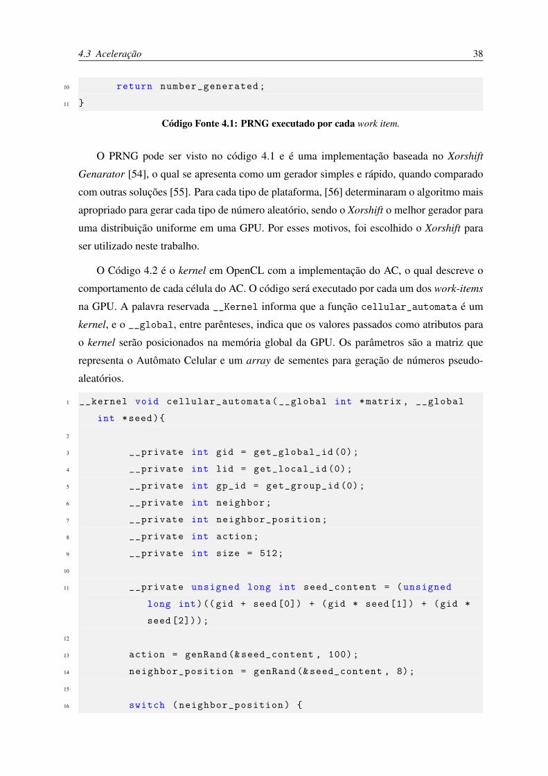
Código Fonte 4.1: PRNG executado por cada work item.
O PRNG pode ser visto no código 4.1 e é uma implementação baseada no Xorshift
Genarator [54], o qual se apresenta como um gerador simples e rápido, quando comparado
com outras soluções [55]. Para cada tipo de plataforma, [56] determinaram o algoritmo mais
apropriado para gerar cada tipo de número aleatório, sendo o Xorshift o melhor gerador para
uma distribuição uniforme em uma GPU. Por esses motivos, foi escolhido o Xorshift para
ser utilizado neste trabalho.
O Código 4.2 é o kernel em OpenCL com a implementação do AC, o qual descreve o
comportamento de cada célula do AC. O código será executado por cada um dos work-items
na GPU. A palavra reservada __Kernel informa que a função cellular_automata é um
kernel, e o __global, entre parênteses, indica que os valores passados como atributos para
o kernel serão posicionados na memória global da GPU. Os parâmetros são a matriz que
representa o Autômato Celular e um array de sementes para geração de números pseudo-
aleatórios.
1 __kernel void cellular_automata(__global int *matrix , __global
int *seed){
2
3 __private int gid = get_global_id (0);
4 __private int lid = get_local_id (0);
5 __private int gp_id = get_group_id (0);
6 __private int neighbor;
7 __private int neighbor_position;
8 __private int action;
9 __private int size = 512;
10
11 __private unsigned long int seed_content = (unsigned
long int)((gid + seed [0]) + (gid * seed [1]) + (gid *
seed [2]));
12
13 action = genRand (& seed_content , 100);
14 neighbor_position = genRand (& seed_content , 8);
15
16 switch (neighbor_position) {

4.3 Aceleração 39
17 //right
18 case 0:
19 neighbor = gp_id*size +((lid+1)%size);
20 break;
21 // bottom
22 case 1:
23 neighbor = (gp_id +1)%size * size + lid;
24 break;
25 //top
26 case 2:
27 neighbor = ((gp_id - 1 + size) % size) * size +
lid;
28 break;
29 //left
30 case 3:
31 neighbor = gp_id * size + ( (lid - 1 + size) %
size);
32 break;
33 // bottom left
34 case 4:
35 neighbor = ((gp_id + 1) % size) * size + ((lid -
1 + size) % size);
36 break;
37 //top right
38 case 5:
39 neighbor = ((gp_id - 1 + size) % size) * size +
((lid + 1) % size);
40 break;
41 // bottom right
42 case 6:
43 neighbor = ((gp_id + 1) % size) * size + ((lid +
1) % size);
44 break;
45 //top left
46 case 7:
47 neighbor = ((gp_id - 1 + size) % size) * size +
((lid - 1 + size) % size);

4.3 Aceleração 40
48 break;
49 default:
50 break;
51 }
52
53 //Move
54 if (action < 50) {
55 if (matrix[gid] != 0 && matrix[neighbor] == 0){
56 matrix[neighbor] = matrix[gid];
57 matrix[gid] = 0;
58 }
59 }
60 // Reproduce
61 else if (action >= 50 && action < 75) {
62 if (matrix[gid] != 0 && matrix[neighbor] == 0){
63 matrix[neighbor] = matrix[gid];
64 }
65 }
66 // Predate
67 else if (action >= 75 && action < 100) {
68 if (matrix[gid] != 0 && matrix[neighbor] != 0){
69 if ((( matrix[gid] + 1) % 3) == (matrix[
neighbor] %3)) {
70 matrix[neighbor] = 0;
71 }
72 }
73 }
74 }
Código Fonte 4.2: Implementação do Autômato Celular.
4.3.2 sort e count
A contagem é um procedimento trivial em uma configuração sequencial. Basicamente, é
preciso declarar uma ou mais variáveis de contagem que serão incrementadas à medida que o
processo de contagem progride. Em uma configuração paralela, onde temos potencialmente
várias threads, a manutenção das variáveis de contagem é um pouco mais complicado, de-

4.3 Aceleração 41
vido às condições de corrida, ou seja, se um work item tentar incrementar uma posição de
memória, os demais devem aguardar até que a ação seja finalizada, a fim de garantir que
nenhum outro sobrescreva o valor e altere o resultado final. A abordagem simples seria o
uso de operações de incremento atômico. No entanto, tornaria o procedimento de contagem
paralela totalmente ineficiente, uma vez que todas as operações de incremento seriam seria-
lizadas. O OpenCL também não possui nenhuma função para contagem paralela eficiente de
elementos de uma matriz.
A técnica de contagem proposta neste trabalho, foi construída com base em um algo-
ritmo usado para o cálculo paralelo de histogramas, originalmente apresentados em [48]. A
abordagem adotada neste trabalho difere em relação ao procedimento de contagem. Como
no método anterior, começamos por ordenar os elementos. No entanto, no segundo passo,
nós executamos um kernel responsável por detectar onde a sequência do elemento muda.
Esse kernel é executado por uma série de work items iguais aos dos elementos da matriz.
Cada work item irá verificar as posições da matriz correspondentes ao seu global ID e ao seu
global ID+ 1. Se os valores armazenados nessas duas posições forem diferentes, a quanti-
dade de elementos da sequência será igual ao ID do work item. Por exemplo, dado que a
posição n possui o elemento i e a posição n+ 1 possui o elemento j, logo podemos inferir
que existem n+1 elementos do tipo i. Esta situação está ilustrada na Figura 4.2.
Figura 4.2: Sort and count.
O kernel utilizado para a contagem dos elementos, uma vez que a matriz já está orde-
nada, é apresentado no Código Fonte 4.3. Ele recebe como argumento a matriz ordenada e
um array auxiliar de tamanho n+ 1, sendo n a quantidade de espécies presentes no AC. A

4.3 Aceleração 42
representação de espécies através de números inteiros simplifica a contagem porque permite
estabelecer uma relação entre o tipo de elemento e a posição da matriz.
1 __kernel void count(__global int *matrix , __global int *density
){
2
3 int gid = get_global_id (0);
4 private int pivot = matrix[gid];
5 private int next_pivot = matrix[gid +1];
6
7 if(pivot != next_pivot ){
8 density[pivot] = gid+1;
9 }
10 }
Código Fonte 4.3: Kernel count.
A quantidade de espaço alocado para o array auxiliar depende do número de espécies
presentes no AC. Por exemplo, suponha que, no caso mostrado na Figura 4.2, existem apenas
três espécies diferentes, neste caso, a matriz auxiliar deve ter apenas quatro elementos, um
para cada tipo de espécie e um para a quantidade de espaços vazios. Assim, o método
permite um consumo de memória reduzido, no caso em que o número de espécies diferentes
é conhecido com antecedência. Também é possível utilizar esta técnica quando não se sabe
previamente a quantidade de espécies, mas, neste caso, o espaço alocado deve ser igual à
quantidade máxima possível de espécies que podem existir no AC, ou seja, será o tamanho
do próprio AC, assumindo que existe apenas um elemento de cada tipo.
Quanto ao algoritmo de ordenação, existem muitas implementações paralelas eficientes
na literatura e qualquer uma pode ser utilizada. Uma técnica pode conseguir um melhor
desempenho dependendo dos dados que estiverem sendo manipulados. Para este trabalho
foi escolhido o Bitonic Sort, pois mostrou maior eficiência quando comparado com outros
algoritmos paralelos em um cenário semelhante [57].

Capítulo 5AVALIAÇÃO EXPERIMENTAL E RESULTADOS
Neste capítulo serão apresentados dados sobre aceleração de Autômatos Celulares, ob-
tidos através de diferentes simulações de um AC. Será feito um comparativo entre uma so-
lução sequencial e sua solução equivalente com paralelismo, bem como técnicas utilizadas
para melhorar o desempenho da solução paralela.
5.1 Experimentos
Serão apresentados 3 cenários envolvendo Autômatos Celulares: 1 sequencial e 2 para-
lelos. Para cada um dos 3 cenários, foram realizadas 3 execuções com ACs de diferentes
dimensões, 1282, 2562 e 5122, totalizando 9 experimentos. Para todos os experimentos, os
ACs foram modelados com as mesmas características descritas no Capítulo 4. Em todos os
experimentos, cada Autômato Celular foi executado durante 10 mil ciclos. Quanto aos re-
cursos computacionais, utilizados para a execução dos experimentos que serão apresentados
neste capítulo, estão descritos na Tabela 5.1.
Tabela 5.1: Configuração de hardware e software
CPU Intel R© Xeon(R) CPU E5620 @ 2.40GHz x 4GPU NVidea Quadro 600, 96 cores, 1280MHzOS Ubuntu 14.04 x64
5.1.1 Experimento I - Sequencial
Como ponto de partida, foi realizada uma implementação do AC utilizando uma abor-
dagem sequencial com C++. Esta implementação foi importante para servir como modelo

5.1 Experimentos 44
de referência de um AC convencional, pois um fator essencial na programação paralela é
garantir a consistência dos dados, ou seja, o resultado obtido em uma implementação se-
quencial deve ser reproduzido também em uma implementação paralela. As abordagens são
diferentes, porém, o resultado deve ser o mesmo. Então, esta implementação será usada na
seção de análise dos resultados, como comparativo com as implementações paralelas. Para
esta implementação, também foi coletado o tempo de execução após 10 mil ciclos, utilizando
apenas a CPU, o qual está disposto na Figura 5.1.
1282 2562 5122
0
100
200
300
15
58
256
Dimensão do AC
Tem
po(s
egun
dos)
Implementação em C
Figura 5.1: Tempo de execução do AC sequencial.
5.1.2 Experimento II - PRNG na CPU e interações na GPU
Neste experimento foi utilizado um algoritmo paralelo, implementado com OpenCL,
para atualização de todas as células do AC. Como o OpenCL não fornece nenhum gerador
de números aleatórios, a CPU ficou encarregada de realizar a escolha de todos os números
aleatórios necessários para a simulação e mandar para a GPU, que por sua vez realiza as
ações de forma paralela. A partir deste experimento, deve ser assumido CPU e GPU como
host e device, respectivamente.
Iniciado o experimento, o host se encarregou de gerar o Autômato Celular. Em seguida,
o AC foi posicionado na memória global do device. Sabe-se que para cada elemento (célula)
do AC realizar uma ação, este precisará de um vizinho e a própria ação, os quais são esco-
lhidos aleatoriamente. Portanto, a estratégia utilizada neste experimento se deu por reservar

5.1 Experimentos 45
mais 2 matrizes com as mesmas dimensões do AC. A primeira matriz foi povoada com N2
números entre 0 e 7, correspondentes aos vizinhos. Desse mesmo modo, a CPU gerou mais
N2 números, variando entre 0 e 1, para representar as ações. Após todos os 2N2 números ge-
rados, suficientes para 1 ciclos de execução do AC, a CPU encaminhava à GPU as 2 matrizes.
Uma vez que todos os dados necessários para a execução do ciclo do AC estavam no device
(matriz do AC, matriz dos vizinhos e a matriz com as ações), dava-se início à execução do
algoritmo paralelo.
N2 work itens foram disparados, 1 para cada posição do AC, e agrupados em N work
groups. O próprio identificador do work item (GID) foi utilizado para fazer o mapeamento
da posição da matriz. Nesse sentido, temos que o elemento na posição GID do AC irá tentar
realizar a ação que está armazenada na posição GID da matriz de ações (respeitando as regras
de movimento, reprodução e predação), sobre um dos seus 8 possíveis vizinhos, o qual está
descrito na posição GID da matriz de vizinhos. Utilizando o GID para mapear as posição das
matrizes, consegue-se maximizar o número de acessos coalescidos à memória. Na Figura 5.2
temos um detalhamento do tempo de execução gasto nessa solução durante 10 mil ciclos do
AC.
1282 2562 5122
0
50
100
150
10
39
156
Dimensão do AC
Tem
po(s
egun
dos)
PRNG na CPU e interações na GPU
Figura 5.2: Tempo de execução do experimento II.

5.1 Experimentos 46
5.1.3 Experimento III - PRNG e interações na GPU
Este experimento é uma melhoria do algoritmo utilizado no caso anterior. Aqui foi
aplicado o PRNG na própria GPU, objetivando reduzir a carga de trabalho do host e a co-
municação entre host e device. As técnicas de aceleração mencionadas na Seção 4.3 foram
aplicadas para este cenário.
1282 2562 5122
0
2
4
6
0.65
1.68
5.8
Dimensão do AC
Tem
po(s
egun
dos)
PRNG e interações na GPU
Figura 5.3: Tempo de execução do experimento III.
O tempo de execução gasto nesta abordagem, durante 10 mil ciclos, pode ser visualizado
na Figura 5.3. Com um PRNG no work item, evitou-se a necessidade de envio dos dados do
host para o device a cada ciclo, o que causou ganhos diretos no desempenho. Ao mesmo
tempo, a carga de trabalho para geração se números aleatórios na CPU foi reduzida, pois
uma parte da implementação pôde ser substituída de sequencial para paralelo.
5.1.4 Análises dos experimentos
5.1.4.1 Experimentos I e II
Como comentado anteriormente, quando algum algoritmo é paralelizado, este deve re-
fletir o resultado da solução sequencial equivalente. Então, o primeiro passo será analisar a
evolução e a formação de padrões entre o experimento sequencial e o paralelo. A Figura 5.4
ilustra as configurações iniciais e finais das duas abordagens. As cores vermelha, verde e azul
representam as 3 espécies concorrentes no experimento, enquanto a cor branca representa os

5.1 Experimentos 47
espaços vazios. As subfiguras (a) e (c) mostram a distribuição aleatória inicial, enquanto (b)
e (d) mostram a estrutura do AC após executar 10.000 ciclos. É importante notar que para os
dois cenários foi utilizada a mesma configuração inicial.
Ambos os cenários refletiram comportamentos semelhantes, sendo possível observar a
formação de padrões e a coexistência entre espécies, resultante das regras aplicadas durante
a modelagem deste AC.
No experimento II o AC é enviado uma única vez, no início da execução, enquanto as
matrizes de vizinhos e de ações são enviadas com novos dados a cada ciclo do AC. A dife-
rença entre a implementação do 2o experimento e a solução sequencial é que, na abordagem
paralela, todas as células do Autômato realizam uma ação no mesmo passo computacional,
N2 células por vez. Enquanto na abordagem sequencial, o AC evolui 1 célula por vez. O
tempo de execução gasto em cada uma das abordagens pode ser visto na Figura 5.5.
5.1.4.2 Experimentos II e III
Temos que no 2o experimento utilizamos o gerador de números pseudoaleatórios (PRNG)
no host, com a função rand pertencente à biblioteca stdlib.h da linguagem C. Enquanto no 3o
experimento, usamos um PRNG maciço no device, com sua própria implementação. Com os
números aleatórios sendo gerados na própria GPU, o gargalo no desempenho produzido pela
transferência de dados entre host e device pôde ser eliminado. A comparação entre os tem-
pos gastos para ambos os experimentos é apresentado na figura 5.6. Ao observar a execução
com AC de tamanho 5122, é possível ver uma considerável diferença de desempenho entre
as abordagens. Enquanto o experimento II necessitava de 2,6 minutos, no experimento III
a execução foi concluída em apenas 5,8 segundos após a inicialização, o que significa uma
aceleração de 26 vezes.
A partir desses dados podemos quantificar a aceleração obtida com o uso de um PRNG
no device. A Figura 5.7 ilustra a aceleração que foi obtida ao adicionar o PRNG no device.
A aceleração a partir do experimento II foi de 15, 23 e 26 para os ACs com dimensões
1282, 2562 e 5122, respectivamente. Em comparação com a implementação sequencial, a
aceleração alcançou até 44x.
5.1.4.3 Sort e Count
O contador apresentado na Seção 4.3.2 foi usado para capturar a evolução da densidade
das espécies a cada 10 ciclos. O resultado pode ser visto na Figura 5.8, onde é possível obser-

5.1 Experimentos 48
(a) Distribuição inicial (b) Aplicação do algoritmo sequencial
(c) Distribuição inicial (d) Aplicação do algoritmo paralelo
Figura 5.4: Formação do Autômato Celular antes e depois de 10.000 ciclos. Comparativo entremodelo sequencial e paralelo.

5.1 Experimentos 49
Figura 5.5: Tempo de execução, experimento I e II.
var um revezamento do domínio entre as espécies. Apesar de ser um cenário de competição,
as três espécies podem coexistir devido a característica cíclica. As cores que representam
a espécie seguem o mesmo padrão que a Figura 5.4, com exceção dos espaços vazios, que
agora são representados pela cor preta.
Conforme mostrado na solução de Sham [48], a operação de contagem deve executar
n(logn)2 operações em média. Esta quantidade é a aproximação do número de comparações
feitas durante a ordenação com Bitonic Sort. No entanto, com a técnica apresentada neste
trabalho, as operações entre contadores podem ser eliminadas. Portanto, uma vez que não
precisamos configurar essas operações dentro do código de ordenação, qualquer algoritmo
pode ser utilizado, incluindo soluções proprietárias de código fechado. Além disso, menos
memória de GPU é gasta, uma vez que não é necessário armazenar contadores para cada
posição da matriz.

5.1 Experimentos 50
Figura 5.6: Tempo de excução, experimento II e III.
1282 2562 5122
10
20
30
40
50
15
2326
23
34
44
Dimensão do AC
spee
d-up
PRNG na GPU
Paralelo com PRNG na CPU Sequencial
Figura 5.7: Speedup do PRNG na GPU.

5.1 Experimentos 51
Den
sity
x10 cycles
0
5000
10000
15000
20000
25000
30000
Figura 5.8: Densidade das espécies durante a simulação.

5.2 Publicações 52
5.2 Publicações
5.2.1 Técnicas de aceleração
As técnicas desenvolvidas nesta pesquisa foram submetidas e aceitas para publicação no
8th Workshop on Applications For Multi-Core Architectures – WAMCA, na linha de Aplica-
ções, Algoritmos e Modelos de Programação. O trabalho que será publicado encontra-se no
apêndice A deste trabalho.
5.2.2 Simulação estocástica de sistemas naturais
O algoritmo desenvolvido nesta pesquisa foi aplicado em um estudo envolvendo Autô-
matos Celulares para a identificação e quantificação do caos em simulações estocásticas uti-
lizadas para estudar a biodiversidade na natureza. O trabalho sugere uma nova abordagem,
baseada no conceito de distância de Hamming e na contagem da densidade de máximos da
abundância das espécies, para a identificação da presença de caos na evolução estocástica
e para quantificar as medidas de correlação através de uma realização experimental simples
com ACs. Os resultados do trabalho podem ser amplamente utilizados para estudar proces-
sos complexos, como os que aparecem em Geologia, Meteorologia, Biologia Evolutiva e em
muitas outras áreas de ciência não-linear. O estudo pode ser encontrado no apêndice B deste
trabalho.

Capítulo 6CONCLUSÃO
Este trabalho buscou aplicar métodos e técnicas computacionais voltados ao processa-
mento de alto desempenho, com computação paralela e GPUs, para aceleração de experi-
mentos na área de Vida Artificial, usando Autômatos Celulares para simulação de sistemas
dinâmicos complexos. O tipo dos dados do objeto de estudo possibilitou adaptações e me-
lhorias dos algoritmos encontrados na literatura. No caso do contador, foi possível chegar na
solução usando menos memória e quantidade de instruções.
A solução apresentada neste trabalho foi capaz de calcular e acompanhar de forma efici-
ente a evolução de um AC. Foi alcançado um speedup de até 26x em relação à implementação
padrão com paralelismo e até 44x quando comparada com uma implementação eficiente em
C. Os experimentos foram executados durante 10 mil ciclos, mas se analisarmos em uma
escala maior, 1 milhão de ciclos por exemplo, essa simulação com o algoritmo sequencial e
com o primeiro algoritmo paralelo, levaria 7 e 4 horas, respectivamente, enquanto que com o
algoritmo apresentado aqui, apenas 9 minutos seriam suficientes. Este aumento de desempe-
nho também é importante para simulações envolvendo matrizes maiores, já que existe uma
complexidade quadrática com relação ao tamanho da matriz.
É importante ressaltar que os resultados foram obtidos com hardware de baixo custo
(como mostrado na Tabela 5.1 do Capítulo 5), sem a necessidade de adquirir componen-
tes caros ou estruturas computacionais sofisticadas como clusters. Como trabalhos futuros,
pretende-se associar a entropia do AC como regra para sua evolução. Para isso, o contador
desenvolvido nesta pesquisa será essencial, uma vez que o cálculo necessitará dos valores
das densidades de cada espécie. Além disso, estima-se que serão necessários bilhões de ci-
clos de execução do AC, ou seja, inviável o uso de computação sequencial ou de alguma
implementação paralela simples.

REFERÊNCIAS
[1] C. G. Langton, Artificial life: An overview. Mit Press, 1997.
[2] Y. Mo, B. Ren, W. Yang, and J. Shuai, “The 3-dimensional cellular automata for hivinfection,” Physica A: Statistical Mechanics and its Applications, vol. 399, pp. 31–39,2014.
[3] A. T. Crooks and A. B. Hailegiorgis, “An agent-based modeling approach applied to thespread of cholera,” Environmental Modelling & Software, vol. 62, pp. 164–177, 2014.
[4] M. Khabouze, K. Hattaf, and N. Yousfi, “Three-dimensional cellular automaton for mo-deling the hepatitis b virus infection,” International Journal for Computational Biology(IJCB), vol. 4, no. 1, pp. 13–20, 2015.
[5] L. Chaves and L. Monteiro, “Oscillations in an epidemiological model based on asyn-chronous probabilistic cellular automaton,” Ecological Complexity, vol. 31, pp. 57–63,2017.
[6] X. Han, B. Chen, and C. Hui, “Symmetry breaking in cyclic competition by nicheconstruction,” Applied Mathematics and Computation, vol. 284, pp. 66–78, 2016.
[7] U. Dieckmann, R. Law, and J. A. Metz, The geometry of ecological interactions: sim-plifying spatial complexity. Cambridge University Press, 2000.
[8] S. Nee, “Evolutionary dynamics: Exploring the equations of life,” Nature, vol. 444, no.7115, p. 37, 2006.
[9] T. Reichenbach, M. Mobilia, and E. Frey, “Mobility promotes and jeopardizes biodi-versity in rock-paper-scissors games,” arXiv preprint arXiv:0709.0217, 2007.
[10] M. Pinsky and S. Karlin, An introduction to stochastic modeling. Academic press,2010.
[11] J. C. Claussen and A. Traulsen, “Cyclic dominance and biodiversity in well-mixedpopulations,” Physical review letters, vol. 100, no. 5, p. 058104, 2008.
[12] C. G. Langton et al., “Artificial life,” 1989.
[13] L. Correia, “Vida artificial,” in XXV Congresso da Sociedade Brasileira de Computa-ção, julho, UNISINOS–São Leopoldo/RS, 2005.

Referências 55
[14] A. M. Turing, “On computable numbers, with an application to the entscheidungspro-blem,” Proceedings of the London mathematical society, vol. 2, no. 1, pp. 230–265,1937.
[15] A. Turing, “The chemical theory of 185. morphogenesis,” Phil. Trans. Roy. Soc. B,vol. 7, 1952.
[16] J. Von Neumann, A. W. Burks et al., “Theory of self-reproducing automata,” IEEETransactions on Neural Networks, vol. 5, no. 1, pp. 3–14, 1966.
[17] W. G. Walter, “An imitation of life,” Scientific American, vol. 182, no. 5, pp. 42–45,1950.
[18] C. Darwin, “On the origin of species,” 1859.
[19] J. H. Holland, “Adaptation in natural and artificial systems. an introductory analysiswith application to biology, control, and artificial intelligence,” Ann Arbor, MI: Univer-sity of Michigan Press, 1975.
[20] S. Wolfram, “Universality and complexity in cellular automata,” Physica D: NonlinearPhenomena, vol. 10, no. 1-2, pp. 1–35, 1984.
[21] J. Santos and Á. Monteagudo, “Study of cancer hallmarks relevance using a cellularautomaton tumor growth model,” in International Conference on Parallel Problem Sol-ving from Nature. Springer, 2012, pp. 489–499.
[22] S. W. McCue, D. G. Mallet et al., “A cellular automata model to investigate immunecell–tumor cell interactions in growing tumors in two spatial dimensions,” in Mathe-matical Models of Tumor-Immune System Dynamics. Springer, 2014, pp. 223–251.
[23] A. K. Cooper and P. S. Kim, “A cellular automata and a partial differential equation mo-del of tumor–immune dynamics and chemotaxis,” in Mathematical Models of Tumor-Immune System Dynamics. Springer, 2014, pp. 21–46.
[24] S. J. McCoy, S. Allesina, and C. A. Pfister, “Ocean acidification affects competition forspace: projections of community structure using cellular automata,” in Proc. R. Soc. B,vol. 283, no. 1826. The Royal Society, 2016, p. 20152561.
[25] B. Kerr, M. A. Riley, M. W. Feldman, and B. J. Bohannan, “Local dispersal promotesbiodiversity in a real-life game of rock–paper–scissors,” Nature, vol. 418, no. 6894, pp.171–174, 2002.
[26] H. Majeed, O. Gillor, B. Kerr, and M. A. Riley, “Competitive interactions in escherichiacoli populations: the role of bacteriocins,” The ISME journal, vol. 5, no. 1, pp. 71–81,2011.
[27] J. J. Arsanjani, M. Helbich, W. Kainz, and A. D. Boloorani, “Integration of logisticregression, markov chain and cellular automata models to simulate urban expansion,”International Journal of Applied Earth Observation and Geoinformation, vol. 21, pp.265–275, 2013.

Referências 56
[28] D. Griffeath, “Self-organizing two-dimensional cellular automata: 10 still frames,” inDesigning Beauty: The Art of Cellular Automata. Springer, 2016, pp. 1–12.
[29] C. Mizas, G. C. Sirakoulis, V. Mardiris, I. Karafyllidis, N. Glykos, and R. Sandaltzo-poulos, “Dna cellular automata,” in Designing Beauty: The Art of Cellular Automata.Springer, 2016, pp. 127–128.
[30] H. Silva and M. Martins, “A cellular automata model for cell differentiation,” PhysicaA: Statistical Mechanics and its Applications, vol. 322, pp. 555–566, 2003.
[31] J. Jackson and L. Buss, “Alleopathy and spatial competition among coral reef inverte-brates,” Proceedings of the National Academy of Sciences, vol. 72, no. 12, pp. 5160–5163, 1975.
[32] B. Sinervo and C. M. Lively, “The rock-paper-scissors game and the evolution of alter-native male strategies,” Nature, vol. 380, no. 6571, p. 240, 1996.
[33] H. Shi, W.-X. Wang, R. Yang, and Y.-C. Lai, “Basins of attraction for species extinc-tion and coexistence in spatial rock-paper-scissors games,” Physical Review E, vol. 81,no. 3, p. 030901, 2010.
[34] P. G. Esteban and A. Rodríguez-Patón, “Simulating a rock-scissors-paper bacterialgame with a discrete cellular automaton,” in International Work-Conference on theInterplay Between Natural and Artificial Computation. Springer, 2011, pp. 363–370.
[35] T. Nagatani, K. Sato, G. Ichinose, and K.-i. Tainaka, “Space promotes the coexistenceof species: Effective medium approximation for rock-paper-scissors system,” Ecologi-cal Modelling, vol. 359, pp. 240–245, 2017.
[36] G. Moore, “Cramming more components onto integrated circuits’, electronics, vol. 38,no. 8,” 1965.
[37] G. E. Moore et al., “Progress in digital integrated electronics,” in Electron DevicesMeeting, vol. 21, 1975, pp. 11–13.
[38] R. Banger and K. Bhattacharyya, OpenCL Programmingby Example. Packt Publishing, 2013. [Online]. Available:https://books.google.com.br/books?id=W2lpAgAAQBAJ
[39] Khronos OpenCL Working Group, The OpenCL Specification, version 1.2 revision 19,2012.
[40] J. Bikker, “Ray tracing for real-time games,” Ph.D. dissertation, TU Delft, 2012.
[41] NVidia, CUDA C Programming Guide PG-02829-001_v8.0, 2017.
[42] AMD, OpenCL User Guide rev1.0, 2015.
[43] J. Caux, P. Siregar, and D. Hill, “Accelerating 3d cellular automata computation with gpgpu in the context of integrative biology,” in Cellular Automata-Innovative Modellingfor Science and Engineering. InTech, 2011.

Referências 57
[44] P. Topa and P. Młocek, “Using shared memory as a cache in high performance cellularautomata water flow simulations,” Computer Science, vol. 14, no. 3, p. 385, 2013.
[45] P. Topa, “Cellular automata model tuned for efficient computation on gpu with globalmemory cache,” in Parallel, Distributed and Network-Based Processing (PDP), 201422nd Euromicro International Conference on. IEEE, 2014, pp. 380–383.
[46] F. NVidia, “Nvidia’s next generation cuda compute architecture,” NVidia, Santa Clara,Calif, USA, 2009.
[47] S. Chen, J. Qin, Y. Xie, W.-M. Pang, and P.-A. Heng, “Cuda-based acceleration andalgorithm refinement for volume image registration,” in BioMedical Information En-gineering, 2009. FBIE 2009. International Conference on Future. IEEE, 2009, pp.544–547.
[48] R. Shams, P. Sadeghi, R. Kennedy, and R. Hartley, “Parallel computation of mutualinformation on the gpu with application to real-time registration of 3d medical images,”Computer methods and programs in biomedicine, vol. 99, no. 2, pp. 133–146, 2010.
[49] C. Vetter and R. Westermann, “Optimized gpu histograms for multi-modal registra-tion,” in Biomedical Imaging: From Nano to Macro, 2011 IEEE International Sympo-sium on. IEEE, 2011, pp. 1227–1230.
[50] J. Gómez-Luna, J. M. González-Linares, J. I. Benavides, and N. Guil, “An optimizedapproach to histogram computation on gpu,” Machine Vision and Applications, vol. 24,no. 5, pp. 899–908, 2013.
[51] R. Shams and N. Barnes, “Speeding up mutual information computation using nvidiacuda hardware,” in 9th Biennial Conference of the Australian Pattern Recognition So-ciety on Digital Image Computing Techniques and Applications (DICTA 2007), Dec2007, pp. 555–560.
[52] P. Avelino, D. Bazeia, L. Losano, and J. Menezes, “von neummann’s and related scalinglaws in rock-paper-scissors-type games,” Physical Review E, vol. 86, no. 3, p. 031119,2012.
[53] G. M. Amdahl, “Validity of the single processor approach to achieving large scalecomputing capabilities,” in Proceedings of the April 18-20, 1967, spring joint computerconference. ACM, 1967, pp. 483–485.
[54] G. Marsaglia et al., “Xorshift rngs,” Journal of Statistical Software, vol. 8, no. 14, pp.1–6, 2003.
[55] R. P. Brent et al., “Note on marsaglia’s xorshift random number generators,” Journal ofStatistical Software, vol. 11, no. 5, pp. 1–4, 2004.
[56] D. B. Thomas, L. Howes, and W. Luk, “A comparison of cpus, gpus, fpgas, and mas-sively parallel processor arrays for random number generation,” in Proceedings of theACM/SIGDA international symposium on Field programmable gate arrays. ACM,2009, pp. 63–72.

Referências 58
[57] F. G. Khan, O. U. Khan, B. Montrucchio, and P. Giaccone, “Analysis of fast paral-lel sorting algorithms for gpu architectures’,” in Frontiers of Information Technology(FIT), 2011. IEEE, 2011, pp. 173–178.

Apendice AAPENDICE A
A seguir encontra-se um paper atualmente aceito para publicação no 8th Workshop on
Applications For Multi-Core Architectures – WAMCA, na linha de Aplicações, Algoritmos
e Modelos de Programação.
Pereira, M. B. P. N., Pagot, Gomes Júnior, J. S., C. A., Ramos, J. G. G. S., Brito, Nas-
cimento, T. P. & A. V., De Oliveira, B., (2017). Acceleration of Cellular Automata through
Parallel Computing with OpenCL.

Acceleration of Cellular Automata through Parallel Computing with OpenCL
Maelso Bruno Pacheco Nunes Pereira1, Christian Azambuja Pagot1, Josue da Silva Gomes Junior1,Jorge Gabriel Gomes de Souza Ramos2, Tiago P. Nascimento1, Alisson V. Brito1
1Centro de Informatica - CI2Departamento de Fisica
Universidade Federal da Paraiba - UFPBJoao Pessoa, Brazil
Email: [email protected], [email protected], [email protected]
Abstract— Cellular Automata (CA) have its origins in thework of Von Neumann and, since then, have become animportant research topic with a wide range of applications,ranging from DNA sequencing to ecological dynamics. Oneaspect that may be of interest during a CA simulation is theevolution in the number of individuals of each species alongtime. This analysis can give important information about thedominance of certain species in a dynamical system, or identifyaspects that might favor one or more species in detrimentof others. CA simulations can be computationally expensivetasks. Depending on the simulation domain size, number ofdimensions or the number of individuals, these simulations cantake several hours to complete. The evaluation of the numberof individuals at each simulation step is an equally expensivetask. Several acceleration techniques have been developed toimprove the performance of CA simulations, and some of themtake into account the evolution in the number of individualsalong the simulation. In this work we propose an efficient CAsimulator which is capable of efficiently evaluate the evolutionin the number of individuals of each species. High performanceis obtained through the use of the massive parallelism of GPUs.The presented approach achieved a speed-up of 44 times whencompared to a sequential implementation, and 26 times whencompared to a traditional approach also in GPU.
I. INTRODUCTION
Cellular Automata (CA) idealized by Ulam and Jonh VonNeumann in the 40s and published by Burk [1], consistsof a self-replicating abstraction model of living organisms,for complex system simulation. A CA is represented by ann-dimensional grid of cells, where each cell of this grid isoccupied by an automaton. Mainly addressed during Com-puter Theory studies, they are finite state machines, whichreceive a stimulus, execute a transition rule or function, andchange state. Each cell in the network can be in any of thepossible existing states, which are updated periodically underthe same rules. The state of a cell is affected by neighboringcell states as they interact with each other.
CA are often used to represent dynamic evolutionarysystems. The configurations produced help us understand themechanics of formation, propagation and pattern interactionin natural systems. Among the applications using CA thereare, interactions between bacteria [2] [3], study of tumorgrowth [4] [5] [6], ecological dynamics [7], self-organization[8], modeling of DNA sequence [9], etc.
The computational progress in relation to the computingpower and data storage has increased the diversity of researchon this field. Recently, parallel computing has allowed thedevelopment of more elaborate systems, since many-coresarchitectures (ie. Graphics Processing Units (GPUs)) are nowbeing used to accelerate such simulations. The simulation ofCellular Automata (CA), including counting the number ofeach species at certain frequency is an expensive computa-tional task. Several acceleration techniques have been devel-oped to improve the performance of CA simulations, andsome of them take into account the evolution of the numberof individuals along the simulation [10][11][12][13][14].
For some applications, like study of species evolution,equilibrium and competition, is essential to know how manyspecie there are in the simulation. This would be a trivial taskfor a sequential implementation, but is it not for a parallelone. In this work we propose a parallel implementation of aCellular Automaton simulator running on GPU, programmedin OpenCL. We present an efficient approach to count thenumber of species at each 10 simulation cycles, whichresulted in an acceleration of 44 times compared to thesequential version of the same CA, and 26 times comparedto a traditional approach implemented in the same GPU. Thisapproach was applied in another work to validate a methodto characterize chaotic systems [15].
II. RELATED WORK
The simulation of CA and the tracking the quantity of eachspecie are problem that demand the implementation of otherimportant features, such as the massive generation of pseudo-random numbers and the ordering of species to acceleratethe counting. In the literature is possible to see an specialconcern related to the problem of massive generation ofnumbers. The massive generation of pseudo-random numbersis recurring in some systems, such as the Cellular Automataand evolutionary systems. It is seen in the literature aconcern in the generation of pseudo-random numbers, suchin the quality of the distribution, as in obtaining gain ofperformance.
The work of Salmon [16] presents an API for gener-ating pseudo-random numbers, using a multi-stream andsub-stream approaches. In the multi-stream approach, the

applications use K as a single key for each computationalunit and generate their own set of pseudo-random numbersin parallel by incrementing their own counters. In the sub-stream approach, the applications split and share the counteramong all computing unit, which generate their own pseudo-random number, using the same key.
In [17], the authors suggest an implementation of theMersenne Twister (MT) algorithm in parallel using CUDA.MT is one of the most well-known and tested pseudo-randomnumber generation algorithms. It presents some character-istics such as: efficient memory usage, good distributionand high performance. In [18] is presented a library forgenerating pseudo-random numbers in CPU and GPU, inaddition to a comparative study between existing librariesand the proposed one applying Monte Carlo simulations. In[19] a pseudo-random number generator is presented basedon the worst case of lattice problems, and GPU tests havereached results close to expected based on the theoreticalreference values.
The other important feature is to calculate the numberof species at each simulation time-step. Some works havededicated to calculate this number in order to verify if in acompetition system, a specie goes extinct or there may becoexistence between them [20], or to analyze the spread rateof infectious agents [10][11][12][13] and to identify factorsthat favor or disfavor species [14].
Other works calculate the number of elements to generatehistograms [21] [22] [23]. In our work, we implement anaccelerated approach to count the number of species basedon the technique presented by [21], which is an advance inrelation to a previous solution [22]. In that work, an extravariable is assigned for each elements of the matrix. In ourapproach, the identification number of the work item is usedinstead, saving memory spaces.
III. PARALLEL PROGRAMMING WITH OPENCL
Meant initially to accelerate graphics applications, theGraphics Processing Units (GPUs) have quickly evolved intomassively parallel processors capable of executing generalpurpose computations. Among the frameworks currentlyavailable for GPU programming, CUDA and OpenCL arethe most popular. CUDA is proprietary and meant to be usedwith NVidia GPUs. OpenCL, on the other hand, is an openand cross-platform standard designed for the programmingof heterogeneous hardware. In this work we have opted forusing the OpenCL framework.
The execution model assumes that the OpenCL work-items(a.k.a. threads) are elements of an n-dimensional indexablespace called NDRange [24]. Each work-item representsone instance of an OpenCL kernel, actually a function tobe executed in a OpenCL device, and they are normallygrouped into work-groups. Work-items are split across theOpenCL platform such that all work-items of a work-groupget assigned to the same compute unit. Also, work-items inthe same work-group can be synchronized through the use ofbarriers and fences. The only way to synchronize work-items
located in distinct work-groups is to start the execution of anew kernel.
The memory model describes the hierarchical OpenCLmemory structure. At the lowest level there is the globalmemory, which will be usually associated to the largestchunk of memory available on the device. It can be readand written by any work-item in execution and will usuallypresent the higher latency. The constant memory is a read-only, and usually very small, piece of memory that is heavilycached. The constant memory is usually used to store smallamounts of data that must be read very frequently by thework-items. The constant memory can only be written, i.e.initialized, by the host and its contents persist along thekernel calls.
The local memory is a small piece of read-write memorylocated at each compute unit. Work-items residing in thesame work-group (thus, being executed by the same computeunit) might use the local memory to exchange information.Currently, there is no way for work-items located in dis-tinct work-groups to exchange information through the localmemory. In this case, the work-items must resort to theslower global memory, which is visible to all work-items.Private memory, in the form of registers, are the fastestmemory available, and can be read and written only by thecurrent work-item. Registers are usually used to store localvariables, including static arrays.
A. Performance
In order to take full advantage of the massive parallelismof the GPU we have to keep all its processing elementsas busy as possible, maximizing utilization. Utilization canbe defined as the percentage of processing elements thatare active in a given instant of time. Among the factorsthat might affect the utilization, we could mention the datalocality, the code execution average flow path, the number ofregisters used by the kernel, among others. The hardware ofthe GPU is optimized for coalesced memory access, i.e. whenwork-items with sequential IDs access sequential memorypositions.
Certain subgroups of work-items are executed in SIMDfashion. Execution flow path divergence among work-itemsin these subgroups causes the execution of all divergingwork-items to be serialized by the GPU. These subgroupsare not actually clearly defined in the OpenCL specification,but correspond to warps on the NVidia nomenclature [25]or wavefronts in the AMD specification [26]. Thus, it isadvisable to avoid flow path divergence among work-items,specifically to those pertaining to those specific subgroups.
Although the maximum number of work-items per workgroup is prescribed by each vendor, theses numbers areusually based on best cases. Since the number of registersavailable is limited, the actual maximum number of work-items per work group will depend on the number of availableregisters and the number of registers needed by the kernel.Thus, it is advisable to always keep the number of privatevariables of the kernel at a minimum such that more work-items can be executed simultaneously.

IV. IMPLEMENTATION
The design of CA can be parameterized by several factors,including dimension, number of cells, neighborhood type,number of species and the types of interactions betweenthem, among others. This work is focused on bidimensionalCA, nonetheless, the extension of the concepts herein pre-sented to higher dimensional CA is straightforward.
The basic interactions will involve mobility, reproductionand predation, each one occurring randomly with the fol-lowing prescribed probabilities: mobility = 0.5, reproduction= 0.25 and predation = 0.25. The range of the interactionsis local and described by the Moore’s neighborhood. Weassume that the lattice present cyclic boundary conditions,i.e. the neighborhood of cells at the boundaries will includecells at the opposite boundary. Figure 1 shows a selectedindividual (black) and the cells with whom it may interactwith (gray). The remaining cells (white) are unreachable.
Fig. 1. Range of interactions
Each simulation timestep comprises four steps, in thefollowing order: 1) cell selection; 2) neighbor selection; 3)selection of interaction type and, finally, 4) lattice update.Initially, a cell L[i, j] is randomly selected from the lattice.If L[i, j] is empty, no changes are applied to the lattice andthe current simulation time-step is finished. If L[i, j] is notempty, a neighboring cell L[s, t] is randomly selected. Inthe next step, one of the three possible interaction types israndomly selected according to their probabilities and it isverified if the selected interaction type (I) is valid for L[s, t].If it is valid, it is executed according to a cyclic competitionsystem [27] and the lattice is updated. If it is not valid, nochanges are applied to the lattice and the current simulationtime-step is finished. Details regarding the interaction typevalidity and lattice update are presented in Algorithm 1. Afterthe execution of these four steps, we say that one interactionhappened in the system. At the end of L2 interactions, onecycle is counted.
A. OpenCL Implementation
We are interested in improving the performance of CAsimulations through the use of massively parallel hardware.In this case, the usual approach is to have as many work-items as cells in the lattice, being each work-item responsiblefor the computations involving its corresponding cell. Whilein the sequential approach the CA evolves a cell at a time, in
Algorithm 1 Check the validity of interactions and updatelattice
1: procedure CHECKVALIDITYUPDATE(L, I , i, j, s, t)2: if I == Move then3: if L[s, t] == ∅ then4: L[s, t]← L[i, j]5: L[i, j]← ∅6: end if7: else if I == Reproduce then8: if L[s, t] == ∅ then9: if ExistNeighborSameSpecies(L[i, j]) then
10: L[s, t]←CreateIndividual(L[i, j].species)11: end if12: end if13: else if I == Predate then14: if L[i, j].species != L[s, t].species then15: if Predate(L[i, j], L[s, t]) then16: L[s, t]← ∅17: end if18: end if19: end if20: end procedure
the parallel approach all Automaton cells perform an actionon the same computational step, L2 cells at a time.
Despite the higher latency of the global memory, asalready discussed in Section III, it was the memory cho-sen to store the lattice due two main reasons. First, itslarger capacity allows for the storage of larger lattices. Thisis specially important in the case of higher dimensionalCA, where memory demands increases exponentially withdimension. Second, it reduces memory consumption andthe complexity of the simulation algorithm. Some methodsadvocate the use of the faster local memory in an attemptto increase performance. Since the lattice will usually notfit into the smaller local memory, it must be broken intosmaller pieces, or tiles. These tiles can now be loaded into thelocal memories where they can be processed in parallel, butindependently by distinct work-groups. The fact that tiles areprocessed independently poses a problem to CA simulationsbecause, in this case, the domain continuity assumption isviolated and alterations occurred in a given tile will notpropagate to the rest of the lattice. The usual approach, inthis case, is to replicate the boundary cell information toother tiles. Despite the effectiveness, this approach implieshigher memory consumption. Additionally, intricate synchro-nization strategies must be employed in order to allow forthe proper propagation of lattice changes among tiles. Thehigher computational demands associated to this approachwill usually outperform the benefits obtained with the use oflocal memories, as already observed by Topa [28].
According to the OpenCL execution model, work-itemsmust be further grouped into work-groups. Since the latticeis stored in the global memory, we should group work-itemssuch that we could benefit from coalesced memory access.Thus, following the approach presented by Topa [28], we

have decided to group, under the same work-groups, work-items sharing the same row in the lattice.
In the first version of our simulator, the host was respon-sible for computing the initial state of the lattice L andfor generating, before each simulation timestep, a neighborpositions matrix G and a interaction matrix I . Right beforethe first timestep, the three matrices should be sent to theGPU which, in turn, would evaluate the first interactionevaluating the interaction between the lattice element L[i, j]and its selected neighbor L[G[i, j]] according to the selectedinteraction I[i, j]. From the second simulation timestep on,only G and I needed to be recomputed by the CPU andsent to the GPU. Despite its effectiveness and improvedperformance over sequential simulators, this approach isstill quite inefficient due the need of constant data transfersbetween the CPU and the GPU. Thus, a second versionof the simulator, which completely avoids data transfersbetween CPU and GPU, was developed. Its implementationis described in the next section.
B. Improved CA Simulator
1) Pseudo-Random Number Generator: The performanceof our first simulator is greatly affected by the constantdata transfers between CPU and GPU. In order to eliminatethis communication, work-items themselves should be ableto randomly select neighboring cells and interaction types.Thus, a framework targeted at the generation of pseudo-random numbers in massively parallel environments wasimplemented.
2) Sort and count: Counting is a trivial procedure in asequential setting. Basically, one has to declare one or morecounting variables which will be incremented as the countingprocedure progresses. In a parallel setting, where we havepotentially several counting threads, the maintenance ofcounting variables is a little more tricky due race conditions.The naïve approach would be to use atomic incrementoperations. However, it would render the parallel countingprocedure totally inefficient, since all increment operationswould be serialized.
The counting procedure proposed in this work was builtupon an algorithm used for the parallel computation ofhistograms originally presented in [21]. According to thisalgorithm, for each position in a matrix there is, in additionto its value, a counter which is initialized to one. Duringthe execution of the sorting algorithm, if two neighboringelements are identical, the one on the right receives the valuestored in the counter of the on the left, while this one receiveszero. When the sorting is finished, all counters related to asequence are zeroed, with the exception of the last one, whichwill contain the number of elements in the sequence.
The approach adopted in this work is similar to that of[21], but differs with respect to the counting procedure. Asin the previous method, we start by sorting the elements.However, in the second step, we execute a kernel thatis responsible for detecting where the element sequencechanges. This kernel is executed by a number of work-itemsequal to that of the matrix elements. Each work-item will
check the matrix positions corresponding to its global ID andits global ID + 1. If the values stored at these two positionsare different, the density of elements of the sequence is equalto the work-item ID + 1. For instance, suppose that theposition n of the matrix contains the value i and positionn + 1 contains j. Thus, we can infer that there are n + 1elements of type i. This situation is illustrated in Figure 2.
Fig. 2. Sort and count
The kernel used for counting is presented in the Listing 1.Its arguments are the sorted matrix and an auxiliary arraycontaining n + 1 elements, being n the total number ofspecies in the CA. The representation of species throughintegers simplifies counting because it allows to establish arelationship between the element type and array position.
The amount of space allocated for the auxiliary arraydepends on the number of different species present in the CA.Thus, the method allows for reduced memory consumptionin the case where the number of different species is knownin advance. For instance, suppose that in the example shownin Figure 2 there are only three different species. In thiscase, the auxiliary array must have only four elements, onefor each type of species and one for the amount of emptyspaces. The proposed method can be used also in situationswhere the number of species is not known in advance. Inthis case, however, the auxiliary array must have a numberof elements that match that of the lattice.
Listing 1. Kernel count1 _ _ k e r n e l vo id c o u n t ( _ _ g l o b a l i n t ∗
mat r ix , _ _ g l o b a l i n t ∗ d e n s i t y ) {2
3 i n t g i d = g e t _ g l o b a l _ i d ( 0 ) ;4 p r i v a t e i n t p i v o t = m a t r i x [ g i d ] ;5 p r i v a t e i n t n e x t _ p i v o t = m a t r i x [
g i d + 1 ] ;6
7 i f ( p i v o t != n e x t _ p i v o t ) {8 d e n s i t y [ p i v o t ] = g i d +1;9 }
10 }
With respect to the GPU-based sorting algorithm, thereare several possibilities, and any of them could have beenused. Depending on how the elements are distributed over the

lattice, some algorithms may perform better than others. Inthis work, we have used the Bitonic Sort algorithm, becauseit has shown better performance with respect to others insimilar scenarios [29].
V. RESULTS
We have implemented the CA with the features describedin Section IV, for 3 different dimensions, 1282, 2562, and5122. One of the executions is illustrated in the Figure 3. Thered, green and blue colors represent the 3 competing speciesin the experiment, while the white color represents the emptyspaces. The first image shows the initial random distribution,while the second image shows the structure of the CA afterexecution for 10,000 cycles. It is possible to observe theformation of patterns and the coexistence between species,this is a result of the rules applied during the modeling ofthis CA.
Fig. 3. Cellular Automata formation before and after 10,000 cycles
For each of the 3 sizes of the CA implemented, we did acomparison between 2 scenarios. In the first scenario, weused Pseudo-Random Number Generator (PRNG) on thehost, with the rand function belonging to the stdlib.h libraryof the C language. In the second scenario, we used a massivePRNG in the device, with its own implementation. Bothscenarios used the same computational resources describedin Table I.
TABLE IHARDWARE AND SOFTWARE CONFIGURATION
CPU Intel R© Xeon(R) CPU E5620 @ 2.40GHz × 4GPU NVidea Quadro 600, 96 cores, 1280MHzOS Ubuntu 14.04 x64
In the second scenario, the numbers were generated by thedevice and the communication bottleneck generated by thebus could be eliminated. Figure 4 is a chart illustrating thenecessary time to compute all simulations for the 3 differentsizes of CA. By observing the execution with 5122 species,it can be seen a wide performance difference between theapproaches. For example, the simulation of CA with 5122
species consumed 256 seconds in the sequential version,while 156 seconds using GPU with traditional approach tocount species (scenario 1), and only 5.8 seconds using ourapproach. This means our approach achieved a speed-up of26 times in comparison with traditional GPU approach. This
speedup was 15 and 23 for CA with 1282 and 2562 species,respectively.
1282 2562 5122
0
100
200
300
15
58
256
1039
156
0.65 1.68 5.8
Cellular Automata size
Tim
e(s
ec)
Time to compute 10 thousand cycles
SequentialTraditional approach in GPU
Our approach in GPU
Fig. 4. Performance comparison to simulate 10 thousand cycles in automatawith 3 different sizes.
The counter presented in Section IV was used to capturethe evolution of species density every 10 cycles. The resultcan be seen in Figure 5. Where it is possible to observe arotation of the dominion between the species. This resultwould not be achieved in practical time if an inefficientapproach were used. Our approach enabled to count speciesduring the simulation, without prejudice considerably thetotal time. Another important result is the observation anexpected behavior present in nature.
Although the initial aleatory configuration and execution,the equilibrium tend to be achieved. Despite it is a compe-tition scenario, the three species can coexist due to cyclicalcharacteristics. The colors representing the species follow thesame pattern as the Figure 3, with the exception of the emptyspaces, which are now represented by black color. Thisbehavior validates our simulations and opens the opportunityto experiment and validate other theories. In [15] we proposea method to characterize chaotic systems, and the simulationpresented here was important to validate this method.
Den
sity
x10 cycles
0
5000
10000
15000
20000
25000
30000
Fig. 5. Density of species during simulation
As shown in the solution of Sham [21], the counting

operation must run n(log n)2 operations in average. Thisquantity is the approximation of the number of comparisonsmade during sorting with Bitonic Sort. However, with thetechnique presented in this work, operations between coun-ters can be neglected. Therefore, since we do not need toset these operations within the sort code, any sorting can beused, including proprietary solutions. In addition, less GPUmemory is spent, since it is not necessary to store countersfor each array position.
VI. FINAL CONSIDERATIONS
In this work we propose an efficient Cellular Automata(CA) simulator accelerated by GPU through the usage of anparallel implementation in OpenCL. the presented solution iscapable of efficiently calculate the evolution in the numberof individuals of each species. Our approach opens the op-portunity to amplify the research about species competition,evolution, adaptation, etc.
The evaluation of the number of individuals at each 10simulation steps is an expensive task, which was mitigatedin this work. Our approach demonstrated to be an efficientCA simulator which is capable of efficiently evaluate theevolution in the number of individuals of each species. Evenexecuting the simulation in regular GPU (96 cores) the timeto execute 10 thousand cycles of a Cellular Automatonwith 5122, also counting species at each 10 cycles wasconsiderably short, only 5.8 seconds. This means a speed-up of 26 times when comparing with traditional approach tocount elements running in the same GPU. This enables thesimulation of even larger CA if GPU with larger memory isused.
REFERENCES
[1] J. Von Neumann, A. W. Burks et al., “Theory of self-reproducingautomata,” IEEE Transactions on Neural Networks, vol. 5, no. 1, pp.3–14, 1966.
[2] B. Kerr, M. A. Riley, M. W. Feldman, and B. J. Bohannan, “Localdispersal promotes biodiversity in a real-life game of rock–paper–scissors,” Nature, vol. 418, no. 6894, pp. 171–174, 2002.
[3] H. Majeed, O. Gillor, B. Kerr, and M. A. Riley, “Competitive inter-actions in escherichia coli populations: the role of bacteriocins,” TheISME journal, vol. 5, no. 1, pp. 71–81, 2011.
[4] J. Santos and Á. Monteagudo, “Study of cancer hallmarks relevanceusing a cellular automaton tumor growth model,” in InternationalConference on Parallel Problem Solving from Nature. Springer, 2012,pp. 489–499.
[5] S. W. McCue, D. G. Mallet et al., “A cellular automata model toinvestigate immune cell–tumor cell interactions in growing tumors intwo spatial dimensions,” in Mathematical Models of Tumor-ImmuneSystem Dynamics. Springer, 2014, pp. 223–251.
[6] A. K. Cooper and P. S. Kim, “A cellular automata and a partial differ-ential equation model of tumor–immune dynamics and chemotaxis,” inMathematical Models of Tumor-Immune System Dynamics. Springer,2014, pp. 21–46.
[7] S. J. McCoy, S. Allesina, and C. A. Pfister, “Ocean acidificationaffects competition for space: projections of community structure usingcellular automata,” in Proc. R. Soc. B, vol. 283, no. 1826. The RoyalSociety, 2016, p. 20152561.
[8] D. Griffeath, “Self-organizing two-dimensional cellular automata: 10still frames,” in Designing Beauty: The Art of Cellular Automata.Springer, 2016, pp. 1–12.
[9] C. Mizas, G. C. Sirakoulis, V. Mardiris, I. Karafyllidis, N. Glykos, andR. Sandaltzopoulos, “Dna cellular automata,” in Designing Beauty:The Art of Cellular Automata. Springer, 2016, pp. 127–128.
[10] Y. Mo, B. Ren, W. Yang, and J. Shuai, “The 3-dimensional cellularautomata for hiv infection,” Physica A: Statistical Mechanics and itsApplications, vol. 399, pp. 31–39, 2014.
[11] A. T. Crooks and A. B. Hailegiorgis, “An agent-based modelingapproach applied to the spread of cholera,” Environmental Modelling& Software, vol. 62, pp. 164–177, 2014.
[12] M. Khabouze, K. Hattaf, and N. Yousfi, “Three-dimensional cellularautomaton for modeling the hepatitis b virus infection,” InternationalJournal for Computational Biology (IJCB), vol. 4, no. 1, pp. 13–20,2015.
[13] L. Chaves and L. Monteiro, “Oscillations in an epidemiological modelbased on asynchronous probabilistic cellular automaton,” EcologicalComplexity, vol. 31, pp. 57–63, 2017.
[14] X. Han, B. Chen, and C. Hui, “Symmetry breaking in cyclic compe-tition by niche construction,” Applied Mathematics and Computation,vol. 284, pp. 66–78, 2016.
[15] D. Bazeia, M. Pereira, A. Brito, B. De Oliveira, and J. Ramos, “Anovel procedure for the identification of chaos in complex biologicalsystems,” Scientific Reports, vol. 7, 2017.
[16] J. K. Salmon, M. A. Moraes, R. O. Dror, and D. E. Shaw, “Parallelrandom numbers: as easy as 1, 2, 3,” in International Conference forHigh Performance Computing, Networking, Storage and Analysis (SC).IEEE, 2011, pp. 1–12.
[17] V. Podlozhnyuk, “Parallel mersenne twister,” NVIDIA white paper,2007.
[18] L. Y. Barash and L. N. Shchur, “Prand: Gpu accelerated parallelrandom number generation library: Using most reliable algorithms andapplying parallelism of modern gpus and cpus,” Computer PhysicsCommunications, vol. 185, no. 4, pp. 1343–1353, 2014.
[19] P.-L. Cayrel, M. Meziani, O. Ndiaye, R. Lindner, and R. Silva,“A pseudorandom number generator based on worst-case latticeproblems,” Applicable Algebra in Engineering, Communication andComputing, pp. 1–12, 2017.
[20] T. Nagatani, K. Sato, G. Ichinose, and K.-i. Tainaka, “Space promotesthe coexistence of species: Effective medium approximation for rock-paper-scissors system,” Ecological Modelling, vol. 359, pp. 240–245,2017.
[21] R. Shams, P. Sadeghi, R. Kennedy, and R. Hartley, “Parallel compu-tation of mutual information on the gpu with application to real-timeregistration of 3d medical images,” Computer methods and programsin biomedicine, vol. 99, no. 2, pp. 133–146, 2010.
[22] R. Shams and N. Barnes, “Speeding up mutual information computa-tion using nvidia cuda hardware,” in 9th Biennial Conference of theAustralian Pattern Recognition Society on Digital Image ComputingTechniques and Applications (DICTA 2007), Dec 2007, pp. 555–560.
[23] T. Scheuermann and J. Hensley, “Efficient histogram generation us-ing scattering on gpus,” in Proceedings of the 2007 symposium onInteractive 3D graphics and games. ACM, 2007, pp. 33–37.
[24] Khronos OpenCL Working Group, The OpenCL Specification, version1.2 revision 19, 2012.
[25] NVidia, CUDA C Programming Guide PG-02829-001_v8.0, 2017.[26] AMD, OpenCL User Guide rev1.0, 2015.[27] P. Avelino, D. Bazeia, L. Losano, and J. Menezes, “von neummann’s
and related scaling laws in rock-paper-scissors-type games,” PhysicalReview E, vol. 86, no. 3, p. 031119, 2012.
[28] P. Topa, “Cellular automata model tuned for efficient computationon gpu with global memory cache,” in Parallel, Distributed andNetwork-Based Processing (PDP), 2014 22nd Euromicro InternationalConference on. IEEE, 2014, pp. 380–383.
[29] F. G. Khan, O. U. Khan, B. Montrucchio, and P. Giaccone, “Analysisof fast parallel sorting algorithms for gpu architectures’,” in Frontiersof Information Technology (FIT), 2011. IEEE, 2011, pp. 173–178.

Apendice BAPENDICE B
A seguir encontra-se um paper publicado na Scientific Reports, Nature Publishing Group.
Bazeia, D., Pereira, M. B. P. N., Brito, A. V., De Oliveira, B., & Ramos, J. G. G. S.
(2017). A novel procedure for the identification of chaos in complex biological systems.
Scientific Reports, 7.

1Scientific RepoRts | 7:44900 | DOI: 10.1038/srep44900
www.nature.com/scientificreports
A novel procedure for the identification of chaos in complex biological systemsD. Bazeia1, M. B. P. N. Pereira2, A. V. Brito2, B.F. de Oliveira3 & J. G. G. S. Ramos1
We demonstrate the presence of chaos in stochastic simulations that are widely used to study biodiversity in nature. The investigation deals with a set of three distinct species that evolve according to the standard rules of mobility, reproduction and predation, with predation following the cyclic rules of the popular rock, paper and scissors game. The study uncovers the possibility to distinguish between time evolutions that start from slightly different initial states, guided by the Hamming distance which heuristically unveils the chaotic behavior. The finding opens up a quantitative approach that relates the correlation length to the average density of maxima of a typical species, and an ensemble of stochastic simulations is implemented to support the procedure. The main result of the work shows how a single and simple experimental realization that counts the density of maxima associated with the chaotic evolution of the species serves to infer its correlation length. We use the result to investigate others distinct complex systems, one dealing with a set of differential equations that can be used to model a diversity of natural and artificial chaotic systems, and another one, focusing on the ocean water level.
In his book on the origin of species, Darwin settled the foundation of evolutionary biology, foreseen the interplay between non-linearity and stochastic processes. Due to the unpredictability of the systems that evolve driven by natural selection rules, over the years several approaches to investigate the problem have been developed. The general procedure relies on eliminating irrelevant information to deal with the appropriate issue, as one sees, for instance, in the Brownian motion, the Langevin and the Fokker-Planck equations, and the Onsager, Uhlenbeck, and Chandrasekhar theories.
Nowadays, despite the many ways to study complex systems, stochastic simulations have became a universal tool, and have been largely used to investigate collective behavior in nature. Based on a set of simple rules that are assessed randomly, the procedure has been employed in a diversity of scenarios to model and understand the experimental data. For a small set of investigations concerned mainly with biodiversity, see, e.g., the works1–12 and references therein.
Without loss of generality, in this work we consider stochastic network simulations of the May and Leonard type5,7, following two recent investigations, one describing how local dispersal may promote biodiversity in a real-life game8 and the other suggesting that population mobility may be central feature to describe real eco-systems10. These studies develop simulations that engender cyclic competition, which is modeled as in the rock-paper-scissors game, controlled by the simple rules: paper wraps rock, rock crushes scissors and scissors cut paper6. We consider the standard system with three distinct species a, b, and c, identified with the colors red, blue, and yellow, respectively, and one notes an interesting behavior of the stochastic simulations which is the pattern formation, indicating a subjacent law. Thus, the separation between the random and the dynamical and kinematical mechanisms that may perhaps contribute to the temporal evolution is of fundamental importance to its understanding.
The study focuses mainly on the presence of chaos, and we go on motivated by the fact that the mechanisms that control the evolution of the system are capable of imprinting the spatial patterns, with the pattern formation being sensible to subtle changes in the initial conditions, driven by the number of individuals in each species. The subject has been investigated before in many different contexts, with very interesting works being carried out on the chaotic behavior in biological systems and in other stochastic situations. Here we recall the works13–31 that are
1Departamento de Física, Universidade Federal da Paraíba, João Pessoa, Paraíba, 58051-970, Brazil. 2Centro de Informática, Universidade Federal da Paraíba, João Pessoa, Paraíba, 58055-000, Brazil. 3Departamento de Física, Universidade Estadual de Maringá, Maringá, Paraná, 87020-900, Brazil. Correspondence and requests for materials should be addressed to D.B. (email: [email protected])
received: 16 November 2016
accepted: 14 February 2017
Published: 21 March 2017
OPEN

www.nature.com/scientificreports/
2Scientific RepoRts | 7:44900 | DOI: 10.1038/srep44900
closely related to the current investigation. In particular, in refs 13–21 the authors put a great deal of effort into the identification of chaos, but in the current work we suggest a new route, which is based on the Hamming dis-tance concept32, and on the counting of the density of maxima33 of the abundance of the species, which we explain below. Other issues that are considered in refs 22–31 deal with generalizations of the standard three-species sys-tem to consider systems with four or more species, with the addition of other rules that may jeopardize biodiver-sity. Specific possibilities are studied in ref. 24 with the addition of diffusion, which may block the spiral pattern formation due to mobility, and also in ref. 26, when one adds players that never change their strategy, regardless of the neighborhood. Moreover, in the recent work28 the authors investigate how to preserve biodiversity despite the presence of a spatially heterogeneous environment.
There are other studies on the cyclic dominance in evolutionary games, as one can find, for instance, in the recent review27. Some works investigate mechanisms that can be used to describe distinct kind of invasion rates between competing species, to act to jeopardize biodiversity. Specific examples can be found in the recent investi-gations29–31, which can be of direct interest to the current study, as we further comment in the Sec. Results.
We study the system with three distinct species and standard rules of evolution. The main motivation to deal within this well-known environment is to unveil the chaotic behavior incontestably. We move on encouraged by decades of studies in the physics of compound nuclei and nuclear resonances, and more recently by theories developed to investigate mesoscopic systems33, in order to offer a positive answer to this issue. Specifically, we identify the presence of chaos in the stochastic evolution and use it to quantify correlation measurements through a single and simple experimental realization of the system. As we show below, instead of following the standard way to describe the chaotic behavior, we pave a new route, with the result relating the correlation length to the average density of maxima of the abundance or density of individuals of a typical species in the system. It is the main result of the work, and is due to the chaotic properties of the stochastic evolution, which we identify and measure in the current study. We also show that it is a general result and can be used in a diversity of situations, to infer the correlation length of systems that evolve in time chaotically. We first identify the finding, and then illustrate it with two distinct applications, one dealing with a set of first-order differential equations, and the other with the ocean water level.
ResultsWe use stochastic simulations and follow standard procedure to investigate a system with three distinct spe-cies8,10. The approach is implemented in Sec. Methods, and there one includes detailed investigation that allows to develop all the results that we describe in the current Section. In particular, one describes the abundance or density of individuals of all the three species. A typical result appears in Fig. 1, where one uses the Bézier algo-rithm to display in blue the abundance of a given species. It shows a pattern that evolves in time oscillating around an average value, developing an apparently unpredictable number of maxima. As it is known, however, the cyclic behavior shown in the figure is in general required to generate stable evolution in a system described by a set of species that fight among themselves under specific rules. In a relatively short time scale, some species may tend to be suppressed, while others increase their abundance, but the dominance of a typical species over another one changes with the time, decreasing and inverting behavior, inducing an average value in a long time evolution. This cyclic equilibrium behavior is the central issue of the current work, and is used to identify the chaotic behavior even in a single and short time evolution of the system, as it is assured by the maximum entropy principle and the ergodic theorem.
The pattern displayed in Fig. 1 presents a number of maxima that can be related to the correlation length, due to the intrinsic chaotic behavior of the density of individuals. The study allows us to express the main result of the current work in the form
τρ
= .1
6 (1)
It relates the correlation length τ to the average density of maxima ρ of the abundance of a typical species which is illustrated in Fig. 1. The counting of maxima is related to the tendency of the system to return to equilibrium, so the higher the density of maxima, the faster the tendency to approach equilibrium, although the system never relax to the state with the abundance fixed at the corresponding average value. The quantification that appears in
Figure 1. The blue Bézier curve shows the evolution of the abundance of a typical species in the interval in between 35000 and 40000 generations. The curve is built from the data corresponding to the blue species that appears in Fig. 4, as described in Sec. Methods.

www.nature.com/scientificreports/
3Scientific RepoRts | 7:44900 | DOI: 10.1038/srep44900
Eq. (1) is due to the chaotic pattern of the stochastic evolution, which we identify and measure using standard techniques. Before working this out, however, in this Fig. 1 one counts the number of maxima in the interval in between 35000 and 40000 generations to get the average density ρ ≈ 0.0034, compatible with the values indi-cated in Fig. 2 (Top). We then use (1) to get τ ≈ 49, consistent with the value suggested in the inset in Fig. 2 (Bottom). The results displayed in Fig. 2 are obtained from an ensemble of stochastic simulations which we explain in Sec. Methods.
The above expression (1) is of very practical use, because it allows us to infer the correlation length with a sin-gle and simple assessment to the time evolution of the chaotic variable under consideration, being it of natural or artificial origin, so it is of wide applicability. It follows from the identification that the stochastic simulation which is generically used in biodiversity engenders chaotic behavior. To focus on this, in Sec. Methods one describes the numerical procedure to be employed in this work. We then use it to assess the random processes engendered by the dynamical evolution. However, due to the impossibility to directly control the randomness of the simulations, the strategy elaborated follows a procedure which generates two distinct final states starting from initial states that are slightly different from each other.
Owing to quantify the chaotic behavior, we employ the Hamming distance32 to measure the difference between the two final states, which is a simple and appropriate manner to distinguish quantities such as vectors, matrices, etc, and can be illustrated with binary vectors. Since it counts the number of sites in the second vector that do not match with the corresponding sites of first one, the distance between (0,0,0,1) and (1,0,1,1) is two, for instance. We use the Hamming distance H(t) to measure the difference between the two final states, which are now seen as two distinct N × N matrices. In Fig. 3 one displays the Hamming distance density h(t) = H(t)/N2 with the solid green curve that represents an average obtained from a set of 100 simulations, each one starting with a distinct initial state. We recall that it is actually nontrivial to distinguish chaos from randomness, but here one has to emphasize that the new algorithm that we have implemented to account for the Hamming distance, which is described in Sec. Methods, provides the possibility to access the chaotic behavior that underlies the stochastic simulations very clearly.
Figure 2. (Top) The counting of the number of peaks for the three species with the corresponding colors blue, red and yellow, with an almost invisible gray line depicting the fitting curve. (Bottom) The correlation function is displayed for the three species in a long time evolution, showing the general behavior. In the inset, it is depicted for a short time evolution, enough to show the correlation length. The shadow region in the inset displays the standard deviation. See Sec. Methods for details.

www.nature.com/scientificreports/
4Scientific RepoRts | 7:44900 | DOI: 10.1038/srep44900
The behavior that appears in Fig. 3 is a key result of the work. It shows that the Hamming distance density increases smoothly and then converges to a given value inside an interval with very narrow width. It is asymp-totically stable and does not fill the full lattice. For an animated illustration on this, see the video at https://youtu.be/nzLP-XcCvWc. We have implemented other simulations, changing the values of the parameters (m,r,p), the size of the lattice and the number of species in the system, and observed the same qualitative behavior, showing its universality.
As we have further noted, if one modifies the rules that control the time evolution, the profile of the Hamming distance density displayed in Fig. 3 may change drastically. For instance, if the modification of the rules does not jeopardize biodiversity, the Hamming distance density gets the universal behavior shown in Fig. 3. However, if one follows the investigations considered in refs 29–31, for instance, and modifies the rules in order to destroy biodiversity, the Hamming distance density starts increasing, oscillating in the interval [0,1], but it ends up van-ishing in the long run, if the two initial states evolve to become the same final state, or become unit, if the two final states are completely different from each other. The result shows that the asymptotic stability of the Hamming distance density is intrinsically connected with biodiversity. We are now investigating how the amplitude and width of the Hamming distance density behave for three, four and five species, as one increases the mobility to higher and higher values, reaching the region that jeopardizes biodiversity, as firstly shown in ref. 10 and further explored in the more recent works34,35. We hope to offer a detailed investigation on this issue in the near future, emphasizing that the Hamming distance behavior is directly related with the evolution of the abundance of a typ-ical species that is displayed in Fig. 1, which was built from the data corresponding to the blue species that appears in Fig. 4. The results depicted in Fig. 4 are further described in Sec. Methods, and show that the abundance of each one of the three species fluctuates around the same average value, as shown in red, blue and yellow.
Knowing that the stochastic processes engender chaotic behavior, it is of interest to further explore the above result. Here one should ask for the behavior of the system under perturbations, the presence of attractors, the Lyapunov spectrum etc. Instead of this standard route, however, we move forward inspired by the previous study33 and focus attention on counting the density of maxima of the time evolution of the abundance of the species. In this sense, one takes li to describe the abundance of one of the three species i = a (red), b (blue), or c (yellow), and considers the investigation developed at the end of the Sec. Methods to calculate the average density of maxima ρi . The main results are shown in Eqs (5–8), and can be used to write ρi in the form
ρπ
=″
′.
ll
12 (2)
ii
i
2
2
Figure 3. The Hamming distance density is shown in green in a long time interval. It represents an average obtained from a set of 100 simulations, each one starting with a distinct initial state.
Figure 4. Evolution of the abundance of the three species, depicted with the corresponding colors, in the long interval in between 35000 and 40000 generations. The data corresponding to the blue species is used to depict the Bézier curve in Fig. 1.

www.nature.com/scientificreports/
5Scientific RepoRts | 7:44900 | DOI: 10.1038/srep44900
This is another key result of the work, and offers a new quantity that arises from the chaotic behavior imprinted in the stochastic simulations. To verify its validity, we implemented a procedure to create an ensemble of events to obtain the correlation function, which is used to calculate the correlation length. As it is known, the correla-tion length τ is extracted from the correlation function as the width at half height, so we use the fitting function C(t) = cos(κt) to write κτ = π/3, and from Eqs (2) and (7) one gets to
ρ κπ
= .2 (3)
This allows to relate the density of maxima to the correlation length in the form τ ρ= ⟨ ⟩1/(6 ), as we have antici-pated in Eq. (1).
The result offers a way to measure the correlation length from a single experimental assessment to the system under investigation, calculating the average density of maxima, as it is illustrated in Fig. 1. We note that the find-ing nicely connects the top and bottom panels in Fig. 2, since the correlation length which one reads from the inset in the bottom panel in Fig. 2 can be obtained from the value of the density of maxima which one reads from the top panel in Fig. 2, via Eq. (1).
Applications. The investigation described above shows that the result in Eq. (1) is valid in a broader context, and can be used to investigate other systems that develop chaotic behavior. To illustrate this issue, in Fig. 5 one displays how x evolves in time for the deterministic system of first-order differential equations
= − − = + . = . − + .dxdt
y z dydt
x y dzdt
z xz, 0 15 ; 0 2 10 (4)
They are the Rössler equations36, and can be used to model a diversity of natural and artificial chaotic systems. We see from the left panel in Fig. 5, where the behavior of x is shown, that the number of maxima is 17, so the correlation length gives τ = 0.097. This is an excellent result, since using the fitting function for the correlation function displayed in the right panel in Fig. 5, one gets to τ = 0.098.
We move on to examine another system of distinct nature that also evolves chaotically. We focus attention on the ocean water level, with data available from the National Oceanic and Atmospheric Administration. This brings about another illustration, which appears in Fig. 6, displaying in blue the observed water level for the station ID 1770000, Pago Pago, American Samoa. See http://tidesandcurrents.noaa.gov/waterlevels.html?id= 1770000. In the right panel in Fig. 6 one shows the correlation function, visually indicating that the correlation
Figure 5. The blue curve in the left panel describes the x(t) evolution that follows from the set of equations (4). The right panel displays the corresponding correlation function.
Figure 6. The ocean water level for the station ID 1770000, Pago Pago, American Samoa, is shown in the left panel for the period from 01/Aug/2016 - 00h00 GMT to 30/Aug/2016 - 23h59 GMT. The right panel displays the corresponding correlation function.

www.nature.com/scientificreports/
6Scientific RepoRts | 7:44900 | DOI: 10.1038/srep44900
length is around 2 hours. In fact, if one uses the fitting curve it gives τ = 2.0748, and if one counts the maxima that appear in the left panel in Fig. 6 and then uses the result in Eq. (1), one gets to the value τ = 2.0689.
DiscussionIn this work we studied the presence of chaos in a system with three distinct species, that evolve under the stand-ard rules of mobility, predation and reproduction. We first used the Hamming distance density to heuristically characterize the chaotic behavior embedded in the stochastic evolution of the system. The typical result is shown in Fig. 3, and is obtained from the algorithm developed in Sec. Methods, which effectively separates the chaotic behavior from the randomness of the stochastic simulations. The qualitative behavior displayed in Fig. 3 suggests that we investigate how the amplitude and width of the Hamming distance density behave for three, four and five species, as one increases the mobility to higher and higher values, reaching the region that jeopardizes biodiver-sity. Being a quantity that unveil the chaotic behavior, the Hamming distance density may be used as an order parameter to investigate chaos in complex systems. We will report on this issue in the near future.
The finding motivated us to developed a stronger result, unveiling a quantitative approach to the correlation length from a single and simple experimental measurement of the average density of maxima that appear in the abundance of a typical species during the dynamical evolution of the system. The connection between the density of maxima and the correlation length was formulated under the principle of maxima entropy, using an ensemble of events that we developed numerically in Sec. Methods. Since the stochastic simulations here considered are universally used to describe biodiversity in nature, we are then left with the suggestion that chaos is imprinted in biodiversity.
The study unveiled a simple route to obtain the correlation length associated to a given chaotic time evolution, and the simplicity of the procedure makes the result especially relevant to investigate complex chaotic systems. Examples of applications of this result abound, and here we have illustrated its applicability with the deterministic system described by the set of first-order differential equations (4), which are known as the Rössler equations36 and engender the behavior displayed in Fig. 5. Also, we have considered another well distinct complex system, dealing with the ocean water level data that is displayed in Fig. 6.
The main result of this work indicates that a single and simple experimental investigation of the time evolution of a given chaotic quantity allows estimating the correlation length of the corresponding quantity with a very high confidence level. As we have illustrated with some explicit examples, it can be widely used to study complex processes, as the ones that appear in Geology, Meteorology, Evolutionary Biology, and in many other areas of nonlinear science. We hope that the current study may help us to better understand biodiversity and its associated chaotic behavior, inspiring further research on similar issues. In particular, the simplicity of the result suggests that the ergodic hypothesis and the maximization of the entropy are valid for complex biological systems and may serve for other studies on the thermodynamics and statistical properties of such systems.
MethodsIn this work we developed stochastic simulations considering a standard system which is widely used to investi-gate biodiversity in nature. We review the procedure recalling that the simulations are implemented considering the system with three distinct species a, b, and c, identified with the colors red, blue, and yellow, respectively. They evolve according to the three basic rules: mobility (m), reproduction (r), and predation (p). The evolution is car-ried out standardly, taking a square lattice of size N × N, in which the three species and the empty sites (which is identified by e, with the color white) are equally but randomly distributed in the lattice, such that the quantity of individuals of each species (including the empty sites) is L = N2/4, at the initial state. We deal with local dispersion and appropriate mobility. A given site is considered active if occupied by an individual of one of the three active species, and it may interact with one of its eight nearest neighbors, the Moore neighborhood.
As usual, the numerical simulations are performed with periodic boundary conditions. If i stands for a,b or c, and α for a,b,c, or e, mobility and reproduction are represented by iα → αi and ie → ii, respectively. The other rule, predation, follow the rock-paper-scissors game, that is, ab → ae, bc → be, and ca → ce. In this work we take m = 0.5, r = 0.25, and p = 0.25, for mobility, reproduction and predation, respectively, for all the three species. We have considered other possibilities, with m = 0.25, r = 0.25 and p = 0.5, for instance, and no qualitative modifi-cation in the results was found. The dynamical process starts with a random assess to the square lattice, followed by a random selection of one of the three rules and by a random choice of one of the eight neighbors. It is then checked if the assessed site is empty or not: if it is empty, one returns to the lattice to simulate another assess to it; if it contains an individual of one of the three species, one takes the selected rule and uses it with the selected neighbor. To measure the time evolution we use generation, which is the time spent to access the lattice N2 times.
To prepare the initial state, one randomly chooses one among the three species a, b and c, and the empty site e with the same probability, and distributes it in the square lattice. The procedure is repeated N2 times, evenly filling all the sites in the square lattice. A typical initial state is illustrated in the left panel in Fig. 7. One uses it to run the stochastic simulations and get to the final configuration which is displayed in the right panel of Fig. 7. There one sees that the system evolves forming a specific pattern, in which the species organize themselves in spatial portions of the lattice. This is known in the literature, and has been explored in a diversity of contexts, to study diversity and other related behaviors.
In order to unveil the chaotic behavior, we use the stochastic simulations to generate a new algorithm. The procedure goes as follows: one first builds a initial state as done in the left panel in Fig. 7, and makes a copy of it. One uses this initial state to run the simulation to get to the final state, which is then saved. The key point here is that during the time evolution a new file is created, in which one saves every single step used to run it. One then takes the copy of the initial state and randomly selects a lattice site and modifies its content. This new state has the tiniest difference, since among the many lattice sites it has a single site which is different from the initial state already used to evolve in time. With this new initial state, one runs the same simulation already considered,

www.nature.com/scientificreports/
7Scientific RepoRts | 7:44900 | DOI: 10.1038/srep44900
evolving it according to the very same rules, in the same order and pace, as they appear in the saved file. The pro-cedure leads to another final state, which is also saved.
The two final states are different, but the difference has nothing to do with the randomness of the stochastic simulations, being due to the tiniest modification introduced in the second initial state. To infer the presence of chaos, one has to measure the difference between the two final states, generated with the same stochastic rules. Toward this goal, we have developed an algorithm which displays in light green the lattice sites that differ in the two configurations, leaving the other sites empty. In Fig. 8 two snapshots are displayed, one at the initial time in the left panel, with a single almost invisible light green site (which is depicted at the grid center) marking the tiniest difference between the two initial states. The other snapshot is in the right panel, and it shows all the light green sites that mark the difference between the two final states, after implementing the simulations for a long time. The two snapshots show the impact that the subtle modification introduced in the initial state causes in the evolution of the system. The result suggests that the time evolution that appears in the stochastic simulation engenders chaotic behavior. The procedure allowed to introduce the Hamming distance density which we dis-cussed in Sec. Results and displayed in Fig. 3.
To further explore the stochastic network simulations, one investigates how the quantities of individuals Li(i = a,b,c) vary as the system evolves in time. In fact, one uses the densities li = Li/N2 and the results are depicted in Fig. 4, showing that the abundance of each one of the three species fluctuates around the same average value, as shown in red, blue and yellow. They do not add to unit because of the number of empty sites, that fluctuates around a lower value. This happens because the species move, reproduce and predate evenly, while the empty sites enter the game passively. We have run other simulations, starting from an initial state with no empty site, and ended up with final states with the species having abundance similar to the ones displayed in Fig. 4. This shows that the addition or not of empty sites in the initial state does not modify the abundance behavior for long time evolutions. The abundance behavior that appear in Fig. 4 show a substructure which is not present in the
Figure 7. The 500 × 500 square lattice is shown at the initial time (left), and after 2000 generations (right), illustrating the formation of spatial patterns.
Figure 8. An illustration of the Hamming distance at the initial time (left), showing an almost invisible green dot at the center of the lattice, and after 1000 generations (right), indicating how the two states separate from each other.

www.nature.com/scientificreports/
8Scientific RepoRts | 7:44900 | DOI: 10.1038/srep44900
curve depicted in Fig. 1, due to the Bézier algorithmic tool used to smooth its behavior. This is a legitimate pro-cedure, since the substructure that appears in the abundance is due to the intrinsic discreteness of the stochastic approach, having nothing to do with the chaotic behavior present in the process under investigation. The Bézier algorithm that we implement in this work uses as the control points the set of points available from the data, in the time interval used to count the number of maxima.
As can be seen from Fig. 4, the abundance li evolves in time and fluctuates to produce local maximum in the interval [t, t + δt], for sufficiently small δt, so one has ′ >l t( ) 0,i and δ′ + <l t t( ) 0,i where prime stands for the time derivative, such that δ− ″ > ′ >l t t l t( ) ( ) 0i i . The joint probability ′ ″P l l( , )i i can be used to calculate the aver-age density of maxima ρi through the simple route: the probability to find a maximum in the interval [t, t + δt] is proportional to the integral spanning the region defined above, such that
∫ ∫ ∫ρδ
⟨ ⟩ ≡ ″ ″ = ″ ″ ″ .δ
−∞
− ′ ′
−∞
″
tdl dl P l l dl l P l1 ( , ) (0, ) (5)i i
l ti i i i i i
0
0
0i
The fact that the statistical properties of the mean number of individuals of a given species are invariant under time translations indicates that both ′li and ″li have vanishing average values. Moreover, the properties of ′ ″P l l( , )i i can be obtained from the smallest momenta of ′li and ″li , and the variances of ′ ″P l l( , )i i are directly related to the correlation function
δ δ= + .C t l t t l t( ) ( ) ( ) (6)i i i
we can then obtain the several momenta, in particular
δδ
δδ
′ = − ″ = .δ δ= =
l d C td t
l d C td t
( )( )
; ( )( ) (7)
ii
ti
i
t
22
20
24
4
0
The principle of maximum entropy can be used to construct the joint probability distribution for li and its derivatives from the previous equations. After implementing the algebraic calculations, integration on li leads to ′ ″P l l( , )i i which gives
π″ =
′ ″
−
″″
.P l
l l
ll
(0, ) 12
1 exp 12 (8)
ii i
i
i2 2
2
2
The above expressions can be used to write the density of maxima in terms of the correlation function, as we showed before in Sec. Results. One then implement a numerical investigation to obtain an ensemble of events, taking an initial state and running the simulation for a very long time. This is a single event, and it is repeated many times, to get to the ensemble of events, each event being built as the first one, running the simulation from a random initial state within the same time interval. The ensemble is then used to count the number of peaks in li(i = a, b, c) in the simulation. They are depicted in the top panel in Fig. 2, for each one of the three species, and there the values of the average density of maxima are also shown.
The procedure is also used to get the correlation function, which is depicted in the bottom panel in Fig. 2 for all the three species in a long time evolution, showing the expected general behavior, with the periodicity reflect-ing the periodic boundary conditions in the lattice. In the inset we depict the correlation function for a time evolution enough to display the correlation length. One then uses the short time evolution shown in the inset of the bottom panel in Fig. 2 to search for the best fit curve, getting C(t) = cos(κt) where κ = 0.0212, with error lower then 5%, obtained within the least square approach. We emphasize that the natural decaying process present in the correlation function is not of practical significance to calculate the correlation length, since it can be obtained from the short time evolution displayed in the inset in the bottom panel in Fig. 2.
References1. David Tilman, P. K. (ed.) Spatial Ecology: The Role of Space in Population Dynamics and Interspecific Interactions (Princeton
University Press, 1997).2. Ulf Dieckmann, J. A. J. M. & Richard, Law (ed.) The Geometry of Ecological Interactions: Simplifying Spatial Complexity (Cambridge
Studies in Adaptive Dynamics) (Cambridge University Press, 2005).3. Nowak, M. A. Evolutionary Dynamics: Exploring the Equations of Life (Belknap Press, 2006).4. Pinsky, M. A. & Karlin, S. An Introduction to Stochastic Modeling fourth edition edn (Academic Press, 2010).5. May, R. M. & Leonard, W. J. Nonlinear aspects of competition between three species. SIAM Journal on Applied Mathematics 29,
243–253 (1975).6. Sinervo, B. & Lively, C. M. The rock-paper-scissors game and the evolution of alternative male strategies. Nature 380, 240–243
(1996).7. Durrett, R. & Levin, S. Spatial aspects of interspecific competition. Theoretical Population Biology 53, 30–43 (1998).8. Kerr, B., Riley, M. A., Feldman, M. W. & Bohannan, B. J. M. Local dispersal promotes biodiversity in a real-life game of rock-paper-
scissors. Nature 418, 171–174 (2002).9. Kirkup, B. C. & Riley, M. A. Antibiotic-mediated antagonism leads to a bacterial game of rock-paper-scissors in vivo. Nature 428,
412–414 (2004).10. Reichenbach, T., Mobilia, M. & Frey, E. Mobility promotes and jeopardizes biodiversity in rock-paper-scissors games. Nature 448,
1046–1049 (2007).11. Szabó, G. & Fáth, G. Evolutionary games on graphs. Physics Reports 446, 97–216 (2007).12. Claussen, J. C. & Traulsen, A. Cyclic dominance and biodiversity in well-mixed populations. Phys. Rev. Lett. 100, 058104 (2008).13. Nowak, M. A. & May, R. M. Evolutionary games and spatial chaos. Nature 359, 826–829 (1992).

www.nature.com/scientificreports/
9Scientific RepoRts | 7:44900 | DOI: 10.1038/srep44900
14. Mitchell, M., Hraber, P. T. & Crutchfield, J. P. Revisiting the edge of chaos: Evolving cellular automata to perform computations. Complex Systems 7, 89–130 (1993).
15. Mitchell, M., Crutchfield, J. P. & Hraber, P. T. Evolving cellular automata to perform computations: mechanisms and impediments. Physica D: Nonlinear Phenomena 75, 361–391 (1994).
16. Yang, C. B., Cai, X. & Zhou, Z. M. Spatial-temporal correlations in the process to self-organized criticality. Phys. Rev. E 61, 7243 (2000).
17. Sato, Y., Akiyama, E. & Farmer, J. D. Chaos in learning a simple two-person game. Proceedings of the National Academy of Sciences 99, 4748–4751 (2002).
18. Károlyi, G., Neufeld, Z. & Scheuring, I. Rock-scissors-paper game in a chaotic flow: The effect of dispersion on the cyclic competition of microorganisms. Journal of Theoretical Biology 236, 12–20 (2005).
19. Gosak, M., Marhl, M. & Perc, M. Chaos between stochasticity and periodicity in the prisoner’s dilemma game. International Journal of Bifurcation and Chaos 18, 869–875 (2008).
20. Gosak, M., Marhl, M. & Perc, M. Chaos out of internal noise in the collective dynamics of diffusively coupled cells. The European Physical Journal B 62, 171–177 (2008).
21. Nicolis, S. C. et al. Foraging at the edge of chaos: Internal clock versus external forcing. Phys. Rev. Lett. 110, 268104 (2013).22. Szabó, G., Szolnoki, A. & Izsák, R. Rock-scissors-paper game on regular small-world networks. Journal of Physics A: Mathematical
and General 37, 2599–2609 (2004).23. Szolnoki, A. & Szabó, G. Phase transitions for rock-scissors-paper game on different networks. Phys. Rev. E 70, 037102 (2004).24. Peltomäki, M. & Alava, M. Three- and four-state rock-paper-scissors games with diffusion. Phys. Rev. E 78, 031906 (2008).25. Avelino, P. P. et al. Junctions and spiral patterns in generalized rock-paper-scissors models. Phys. Rev. E 86, 036112 (2012).26. Szolnoki, A. & Perc, M. Zealots tame oscillations in the spatial rock-paper-scissors game. Phys. Rev. E 93, 062307 (2016).27. Szolnoki, A. et al. Cyclic dominance in evolutionary games: a review. Journal of The Royal Society Interface 11, 20140735 (2014).28. Szolnoki, A. & Perc, M. Biodiversity in models of cyclic dominance is preserved by heterogeneity in site-specific invasion rates.
Scientific Reports 6, 38608 (2016).29. Juul, J., Sneppen, K. & Mathiesen, J. Labyrinthine clustering in a spatial rock-paper-scissors ecosystem. Phys. Rev. E 87, 042702
(2013).30. Vukov, J., Szolnoki, A. & Szabó, G. Diverging fluctuations in a spatial five-species cyclic dominance game. Phys. Rev. E 88, 022123
(2013).31. Szolnoki, A., Vukov, J. & Perc, M. From pairwise to group interactions in games of cyclic dominance. Phys. Rev. E 89, 062125 (2014).32. Hamming, R. W. Error detecting and error correcting codes. Bell System Technical Journal 29, 147–160 (1950).33. Ramos, J. G. G. S., Bazeia, D., Hussein, M. S. & Lewenkopf, C. H. Conductance peaks in open quantum dots. Phys. Rev. Lett. 107,
176807 (2011).34. Jiang, L.-L., Zhou, T., Perc, M. & Wang, B.-H. Effects of competition on pattern formation in the rock-paper-scissors game. Phys.
Rev. E 84, 021912 (2011).35. Cheng, H. et al. Mesoscopic Interactions and Species Coexistence in Evolutionary Game Dynamics of Cyclic Competitions. Scientific
Reports 4, 7486 (2014).36. Rössler, O. An equation for continuous chaos. Physics Letters A 57, 397–398 (1976).
AcknowledgementsThis work was partially financed by the CNPq Grants 455931/2014-3, 306614/2014-6, 308241/2013-4 and 479960/2013-5.
Author ContributionsM.B.P.N.P., A.V.B. and J.G.G.S.R. organized the numerical procedure. M.B.P.N.P., A.V.B. and B.F.O. implemented the stochastic simulations. D.B., B.F.O. and J.G.G.S.R. analysed the results and organized the figures. D.B. and J.G.G.S.R. wrote the manuscript. All authors reviewed and approved the work.
Additional InformationCompeting Interests: The authors declare no competing financial interests.How to cite this article: Bazeia, D. et al. A novel procedure for the identification of chaos in complex biological systems. Sci. Rep. 7, 44900; doi: 10.1038/srep44900 (2017).Publisher's note: Springer Nature remains neutral with regard to jurisdictional claims in published maps and institutional affiliations.
This work is licensed under a Creative Commons Attribution 4.0 International License. The images or other third party material in this article are included in the article’s Creative Commons license,
unless indicated otherwise in the credit line; if the material is not included under the Creative Commons license, users will need to obtain permission from the license holder to reproduce the material. To view a copy of this license, visit http://creativecommons.org/licenses/by/4.0/ © The Author(s) 2017