MESTRADO

MESTRADO EM CIÊNCIAS EMPRESARIAIS

TRABALHO FINAL DE MESTRADO DISSERTAÇÃO

LOG PERIODIC ANALYSIS OF CRITICAL CRASHES IN THE PORTUGUESE STOCK MARKET

JORGE VICTOR QUIÑONES BORDA

JUNIO - 2015

MESTRADO EM

CIÊNCIAS EMPRESARIAIS

TRABALHO FINAL DE MESTRADO DISSERTAÇÃO

LOG PERIODIC ANALYSIS OF CRITICAL CRASHES IN THE PORTUGUESE STOCK MARKET

JORGE VICTOR QUIÑONES BORDA

ORIENTAÇÃO: MESTRE PEDRO NUNO RINO CARREIRA VIEIRA

DOUTOR PEDRO LUIS PEREIRA VERGA MATOS

JANEIRO - 2016

i

Resumo

O estudo de fenómenos críticos que se originaram nas ciências naturais e encontraram muitos campos de aplicação foi estendido nos últimos anos aos campos da economia de finanças, fornecendo aos investigadores novas abordagens para problemas conhecidos, nomeadamente aos que estão relacionados com a gestão de risco, a previsão, o estudo de bolhas financeiras e crashes, e muitos outros tipos de problemas que envolvem sistemas com criticalidade auto-organizada.

A teoria de singularidades de tempo oscilatório auto-similares é apresentada, uma metodologia prática é exposta, juntamente com alguns resultados de análises semelhantes de diferentes mercados em todo o mundo, como uma maneira de obter de alguns exemplos da forma como a função "linear" log-periódica de potências funciona.

Apresento alguns contextos onde o tempo de crise é apresentado aos mercados internacionais - como uma maneira de demonstração de antecedentes -, assim como apresento também três aplicações práticas do mercado de acções português (1997, 2008 e 2015). A sensibilidade dos resultados e do significado das oscilações log-periódicas são avaliadas.

Concluo com algumas recomendações e futuras propostas de investigação.

ii

Abstract

The study of critical phenomena that originated in the natural sciences and found many fields of applications has been extended in the last years to the financial economics’ field, giving researchers new approaches to known problems, namely those related to risk management, forecasting, the study of bubbles and crashes, and many kind of problems involving complex systems with self-organized criticality.

The theory of self-similar oscillatory time singularities is presented. A practical methodology is exposed along with some results from similar analysis from different markets around the world, as a way to get some examples of the way the ´Linear´ Log-Periodic Power Law formula works.

Some context presenting the international markets at the time of crisis is given as a way of having some background, and three practical applications for the Portuguese stock market are made (1997, 2008 and 2015). The sensitivity of the results and the significance from the log-periodic oscillations is assessed.

It concludes with some recommendations and future proposed research.

Keywords: Financial bubble, Self-organized criticality, Crash, Log-periodic power law, Prediction, Financial Crisis

iii

Acknowledgments

To those that helped me to advance.

"Errors of Nature, Sports and Monsters correct the understanding in regard to ordinary things, and reveal general forms. For whoever knows the way of nature will more easily notice her deviations; and, on the other hand, whoever knows her deviations will more accurately describe her ways" Francis Bacon, Novum Organum

iv

Table of Contents Resumo ........................................................................................................................................... i

Abstract ......................................................................................................................................... ii

Acknowledgments ........................................................................................................................ iii

Table of Contents ..........................................................................................................................iv

List of Abbreviations ......................................................................................................................vi

List of Figures ............................................................................................................................... vii

List of Tables ................................................................................................................................ viii

1) Introduction .......................................................................................................................... 2

2) Literature Review .................................................................................................................. 3

2.1) Market Rationality, Random Walk and Efficiency.............................................................. 3

2.2) Introduction to the Theory of self-similar oscillatory finite-time singularities in Finance 5

2.3) Self Organized Criticality and Market Rationality .............................................................. 7

2.4) Bubbles and Anti-Bubbles .................................................................................................. 7

2.5) Drawdowns ...................................................................................................................... 10

2.6) Feedback, Herding and Imitation ..................................................................................... 11

3) The model: The Log-Periodic Power Law ............................................................................ 14

3.1) Macroscopic Modelling .................................................................................................... 15

3.2) Microscopic Modelling .................................................................................................... 16

3.3) Price dynamics ................................................................................................................. 18

3.4) The LPPL Equation ............................................................................................................ 20

3.5) The Fitting Process and Expected Results ........................................................................ 21

4) Contextual Analysis ............................................................................................................. 23

4.1) 1997-1998 Crisis ............................................................................................................... 23

4.2) 2007-2008 Crisis ............................................................................................................... 23

4.3) 2015 Crisis ........................................................................................................................ 24

5) Data Analysis, Methodology and Results ............................................................................ 26

5.1) Data .................................................................................................................................. 26

5.2) Methodology .................................................................................................................... 26

5.3) Results and Discussion ..................................................................................................... 26

5.3.1) Analysis of the 1998 Crash ........................................................................................ 26

5.3.2) Analysis of the 2007 Crash ........................................................................................ 30

5.3.3) Analysis of the 2015 Crash ........................................................................................ 33

5.3.4) Log-Periodic Analysis of the Data minimizing the Root Mean Squared Deviation ... 37

v

5.3.5) Artificial Series and Critical Time Sensitivity ............................................................. 39

6) Conclusions, Recommendations, Limitations and Future Research ................................... 41

6.1) Main Conclusions ............................................................................................................. 41

6.2) Recommendations ........................................................................................................... 41

6.3) Limitations and Future Research ..................................................................................... 41

References ................................................................................................................................... 42

Appendix ..................................................................................................................................... 46

vi

List of Abbreviations

CDO – Collateralized Debt Obligations

DDM – Dividend Discount Model (also known as the Gordon growth model)

DJIA – Dow Jones Industrial Average

EVT – Extreme Value Theory

GNP – Gross National Product

IMF – International Monetary Fund

MBS – Mortgage Backed Security

LPPL – Log Periodic Power Law

RMSD – Root Mean Squared Deviation

SOC – Self Organized Criticality

SSE CI – Shangai Stock Exchange Composite Index

VaR – Value at Risk

vii

List of Figures

Figure 1: Representation of a) An equilibrated market on a 256x256 plane, b) A market in a Critical State, c) A bubble. Taken from (Sornette, 2003) ............................................................ 15 Figure 2: Representation of a trader as part of a network (Prepared by the Author) ................ 16 Figure 3: Price dynamics, taken from Ide & Sornette (2002, p. 90) ............................................ 19 Figure 4: Log of the SSE CI for the 2013-2015 period. ................................................................ 25 Figure 5: Log(PSI20) for the 96-98 period. .................................................................................. 27 Figure 6: Histogram of the Standardized Residuals for the GARCH (2,2) model for the 96-98 period. ......................................................................................................................................... 27 Figure 7: Results obtained with tlast points ranging from 98.25 to 98.38.................................... 29 Figure 8: Results obtained with tlast points ranging from 98.42 to 98.54.................................... 29 Figure 9: Sensitivity Analysis of the Critical Times tc – 1998 Crisis. ............................................. 30 Figure 10: Log(PSI20) for the 2003-2008 period. ........................................................................ 30 Figure 11: Histogram of the Standardized Residuals for the GARCH (1, 1) model for the 2003-2007 period. ................................................................................................................................ 31 Figure 12: Results obtained with tlast points ranging from 107.04 to 107.16. ............................ 32 Figure 13: Results obtained with tlast points ranging from 107.21 to 107.33. ............................ 33 Figure 14: Sensitivity Analysis of the Critical Times tc – 2007 Crisis. ........................................... 33 Figure 15: Log(PSI20) for the 2012-2015 period. ........................................................................ 34 Figure 16: Histogram of the Standardized Residuals for the GARCH (2, 2) model for the 2012-2015 period. ................................................................................................................................ 35 Figure 17: Results obtained with tlast points ranging from 115.17 to 107.29. ............................ 36 Figure 18: Results obtained with tlast points ranging from 115.34 to 115.46. ............................ 36 Figure 19: Sensitivity Analysis of the Critical Times tc – 2015 Crisis. ........................................... 37 Figure 20: Result obtained for the 1998 crisis minimizing RMSD and using tlast=98.50 (Left). ... 38 Figure 21: Result obtained for the 2007 crisis minimizing RMSD and using tlast=107.29 (Right). 38 Figure 22: Result obtained for the 2015 crisis minimizing RMSD and using tlast=115.42. ........... 38 Figure 23: Critical times generated using the artificial series for the 1998 Crash (Left). ............ 39 Figure 24: Critical times generated using the artificial series for the 2007 Crash (Right). ......... 39 Figure 25: Critical times generated using the artificial series for the 2015 Crash. ..................... 40

viii

List of Tables

Table 1: Summary of the parameters of the Log-Periodic Power Law fit to the main bubbles

and crashes up to 1998, taken from (Johansen & Sornette, 1999) ............................................ 22

Table 2: Fitting of a GARCH (2, 2) Model for the 1996-1998 period. .......................................... 27 Table 3: Fitting of the Log-Periodic “Linear” Model for the 1996-1998 period for samples with different ending points (tlast). ...................................................................................................... 28

Table 4: Fitting of a GARCH (1, 1) Model for the 2003-2007 period. .......................................... 31 Table 5: Fitting of the Log-Periodic “Linear” Model for the 2003-2007 period for samples with different ending points (tlast). ...................................................................................................... 32 Table 6: Fitting of a GARCH (2, 2), using an Auto Regressive Distributed Lag Model with one lag and no intercept as the main equation for the 2012-2015 period. ............................................ 34 Table 7: Fitting of the Log-Periodic “Linear” Model for the 2012-2015 period for samples with

different ending points (tlast). ...................................................................................................... 35

Table 8: Fitting of the Log-Periodic “Linear” Model for the selected ending points for 1998, 2007 and 2015 Crisis, minimizing the RMSD. .............................................................................. 38

2

1) Introduction In this work we will present the theory of self-similar oscillatory finite-time in finance and its application to the prediction of crashes. First we will present some terms and concepts that will be used with regularity, and later we will make a brief introduction to the theory before starting to analyse its different aspects and the challenges concerning the prediction aspect.

In the Literature Review, we will discuss the different points of view regarding market rationality, and its relationship with SOC. In the third chapter we will present the model behind the LPPL formula and some guidelines for its application. In the Contextual Analysis chapter, the most important international actors behind the 1998, 2007-2008 and the 2015 crisis are presented.

The Data Analysis, Methodology and Results will present the results obtained from the analysis of the Portuguese Stock Market in three critical periods (1997, 2007-2008 and 2015). Chapter 6 concludes and presents recommendations and suggestions for future research.

The importance of bubbles and crashes in the stock market has always attracted a lot of interest, given how wealth is created so fast as if it didn´t came from nowhere, just to end abruptly when most economists, forecasters and experts expected the positive trend to continue in an indefinite way.

Bubbles and the way these develop have been present in different markets during different eras, showing common features despite technological changes or differences among countries. In all cases, when the bubble ends, analysts would look for what it caused the crash, and they´ll usually find it, in some piece of news. However, it seems to be that financial markets are unstable by design, and that the oscillations of prices before crashes, could be caused by the way markets are organized. It is possible that the cause of the crashes are the bubbles itself, and the news are just triggers, but the instability has to exist to begin with.

3

2) Literature Review

2.1) Market Rationality, Random Walk and Efficiency Markets are considered efficient if all available information about the assets is reflected in current market prices (Johansen, et al., 2000; Blume & Siegel, 1992), An important aspect of price dynamics is noise trading, being defined as “trading on noise as if it were information” (Black, 1986). In this context, we will consider the effects of the interactions of so-called technical traders and fundamental traders. Technical traders use chartist techniques that attempt to predict future behaviour of stock prices based on the knowledge of the past behaviour of price series (Fama, 1965). It was noted that this assumes dependencies among successive price changes, as well as gives importance to past series of prices for prediction purposes.

Technical trading is in contradiction with the majoritarian opinion that states that the market follows a random-walk. This has been defined as “a market where successive price changes in individual securities are independent” (Fama, 1965, p. 5).

Fundamental analysis is based on the assumption of the existence of an intrinsic value (or equilibrium price) that is based on the potential earnings of the stock, which in turn is based on many different factors (management quality, state of the industry, country situation, etc.). A fundamentalist would determine the intrinsic value, and by its comparison with the market´s price, would determine if it´s over or undervalued. This will then, in fact, represent a prediction of the future path of the stock since an eventual return to the intrinsic price is to be expected (Fama, 1965).

Maximally rational markets are markets where all investors are rational, in that scenario trading volume would be very small and investors would invest mostly in index funds Rubinstein (Rubinstein, 2000). However, since that´s not the world where we live in, we know that markets are not maximally rational. A more realistic approach considers that the markets are rational, understood as a market where “prices are set as if all investors are rational” (Rubinstein, 2000, p. 4). A market like that can be obtained even if not all investors are rational, that is, they can trade in excess or diversify too little. In recent investigations, it has been found that the main features of financial markets (volatility clustering and heavy tails) can be replicated without assuming rationality using the `zero-intelligence’ approach (Thompson & Wilson, 2013). Market efficiency could emerge on a macro level even if market participants behave in an irrational way, since market structure seems to be more important than its participants (Gode & Sunder, 1993) . These conclusions were in line with Farmer et al (2005, p. 2259), who concluded that “institutions strongly shape our behaviour, so that some of the properties of markets may depend more on the structure of institutions than on the rationality of individuals.” Farmer also suggested that rational effects are the ones behind price levels, but that volatility could be related to random fluctuations.

The theory of random walks “implies that a series of stock price changes has no memory-the past history of the series cannot be used to predict the future in any meaningful way” (Fama, 1965, p. 6). He also considers that even when price changes could not have a zero correlation, this could be small enough to ignore, if we are not able to gain abnormal profits by trading on knowledge of the past of the series.

4

The independence assumption among prices, suggested by the random-walk model, has been usually considered a reasonable representation of the behaviour of stock markets given that no complex trading rule has ever proved superior to the simple buy-and-hold1 (Fama, 1965; Tryfos, 2001). Rubinstein (2000) mentions that even if markets are irrational and discrepancies between market prices and fundamental prices are found, that wouldn´t necessarily represent a profit opportunity, if there is no way to exploit the advantage due to market structure, regulations or trading costs. Rubinstein (2000, p. 4) adds that markets “are at least minimally rational: although prices are not set as if all investors are rational, there are still no abnormal profit opportunities for the investors that are rational”.

One problem with Fundamental Analysis is that the fundamental or true price, could never be observed in reality (Blume & Siegel, 1992). This happens because full information is never disclosed and not all investors are equally informed, and because “in an uncertain world the intrinsic value of a security can never be determined exactly” (Fama, 1965, p. 4), however, it could be expected that stock prices wander in a random way around its true value.

According to the rational markets view, price irregularities and systematic patterns are due to mistakes in “the collective judgment of investors” (Malkiel, 2003, p. 80), and those systematic irregularities could persist only for short periods since investors would make it disappear by trying to profit from them For the same reason, individual forecasting models would also show declining value after some time (Timmermann & Granger, 2004). That is, by creating forecasting models that correctly predict the patterns, and by acting on them, the patterns will disappear in time.

According to Romer (1993), there is an extreme efficient-markets view of markets, which considers that all information is processed in a mechanical way and arrives to optimal estimates of fundamental variables. However, given that this extreme view doesn´t perform adequately in empirical tests, a second view emerged, one that considers that markets are irrational and suffer waves of optimism and pessimism not entirely based on news. In addition to those ways of explaining the behaviour of markets, (Romer, 1993, p. 1129) suggested “an intermediate view: that the market is, in effect, engaged in a many-dimensional and a many-agent inference problem with multiple layers of uncertainty and heterogeneity and with frictions in the trading process”. Because of this, market prices are not related in a simple way to news; the process is not direct, and it explains why it could be compatible to have rational investors and price movements without the arrival of news. Talking about this process, Fama (1965), mentioned that instantaneous adjustments would lead to over-adjustments and under-adjustments in the same proportion, and the lag of adjustment to a more precise level would be a random variable.

The ´paradox´ in efficient markets says that markets can only be efficient if there are investors that think that the market is inefficient and spend time and money trying to get information to be able to exploit the perceived inefficiencies (Blume & Siegel, 1992). This is related to the noise traders or liquidity traders, which by their operations, add noise. Their counterparties never know if the initiator of the trade is acting based on information or noise. Through these operations, additional volatility is entered into the

1 After trading commissions.

5

market, and “with a lot of noise traders in the market, it now pays for those with information to trade. It even pays for people to seek out costly information which they will then trade on” (Black, 1986, p. 531). However, if the markets were perfectly efficient, professional investors wouldn´t have incentives to gather information since it would be reflected too quickly in market prices (Malkiel, 2003) .

We are faced with a puzzling situation where even when we know that technical trading couldn’t work due to the efficiency of markets, this is still widely used, even when its basic assumption is that history tends to repeat itself and past patterns will recur at some point in the future (Fama, 1965). However, given that market participants have an effect on market behaviour, we get as a result “a symmetric Nash equilibrium at which the average final wealth of agents in the market is lower than in the hypothetical equilibrium in which everyone uses only fundamental trading rules” (Joshi, et al., 1999, p. 2). Other effects mentioned as a consequence of the use of technical trading is the reduced ability to forecast due to the reinforcement of price trends, an increased volatility and noise, and smaller earnings.

We could be in a prisoner’s dilemma that lands us in a sub-optimal equilibrium, where technical trading is the dominant strategy because “it makes each agent better off regardless of what strategy other traders in the market follow” (Joshi, et al., 1999, p. 15). They consider that even when technical trading would be inevitable, it could be better if it would be possible to avoid it, given that a market where investors follow fundamental trading rules would have a higher optimum.

2.2) Introduction to the Theory of self-similar oscillatory finite-time singularities in Finance

In this framework, markets are considered as open and non-linear complex systems that exhibit emanating patterns (Bastiaensen, et al., 2009) include evolutionary adaptive characteristics and are “populated by bounded rational agents interacting with each other” (Sornette & Andersen, 2002, p. 173)2.

An important property of complex systems is the possible manifestation “of coherent large-scale collective behaviours with a very rich structure, resulting from the repeated nonlinear interactions among its constituents: the whole turns out to be much more than the sum of its parts” (Sornette, 2003, p. 12). Sornette adds that most complex systems can´t be solved, instead should be explored using numerical methods. In most cases, given that the systems are computationally irreducible, their dynamical future time evolution wouldn´t be predictable. Even with the continuous increasing of computing power, prediction of critical events could still be difficult, due to the under sampling of extreme situations (Sornette, 2003).

However, it should be noted that the interest is not in predicting the detailed evolution of systems, but in trying to detect the arrival of critical times and the extreme events (Sornette, 2003). Talking about weather prediction, Lorenz (1972, p. 4), stated that “certain special quantities such as weekly average temperatures and weekly total rainfall

2 Related research includes analysis of epidemics, spread of opinions, large natural catastrophes, social unrest among others (Sornette, 2002).

6

may be predictable at a range at which entire weather patterns are not.”, showing that at that time, even when the complete system could not be solved, some measures could still be anticipated.

Self-Organized Criticality is defined as “the spontaneous organization of a system driven from the outside into a globally stationary state, which is characterized by self-similar distributions of event sizes and fractal geometrical properties” (Sornette, 2007, p. 7013). This stationary state is dynamical and characterized by the emergence of statistical fluctuations that are usually called ´avalanches´. In this context “´criticality´ refers to the state of a system at a critical point at which the correlation length and the susceptibility become infinite in the infinite size limit” (Sornette, 2007, p. 7013), while self-organized is related to “pattern formation among many interacting elements. The concept is that the structuration, the patterns and large scale organization appear spontaneously. The notion of self-organization refers to the absence of control parameters” (Sornette, 2007, p. 7013).

Critical points are points in time where you observer “the explosion to infinity of a normally well-behaved quantity” (Johansen, et al., 2000, p. 1), these situations could be a common occurrence.

The ´Dragon King´ concept was proposed by Sornette, where the term ´king´ is used “to refer to events which are even beyond the extrapolation of the fat tail distribution of the rest of the population” (Sornette, 2007, p. 7018).

Endogeneity in stock markets, what according to according to Sornette & Cauwels (2014) is known as ´reflexivity´ by George Soros, is defined as “the fraction of transactions that are triggered internally or are self-excited, (…) and that are not the result of some new external information” (Sornette & Cauwels, 2014, p. 123).

Inside the SOC framework, stock market crashes are due to “the slow build-up of long-range correlations” (Johansen, et al., 2000, p. 220), and the markets eventually land into a crash because those correlations lead to a global cooperative behaviour (Kaizoji & Sornette, 2008). This theory can be applied equally to bubbles ending in a crash and to those that land smoothly (Johansen, et al., 1999).

The forecasting of crashes is compatible with rational markets, because even if investors know that there is a high risk of a crash, this crash could happen anyway, and investors would not be able to earn any abnormal risk-adjusted return by the use of this information (Johansen, et al., 2000), because “investors must be compensated by the chance of a higher return in order to be induced to hold an asset that might crash” (Johansen & Sornette, 1999, p. 3). That is, the price of the assets go up, but that´s rational because the risk of a crash has increased.

The similar patterns arising before crashes at different times, have been attributed to the stable nature of humans, since they are essentially driven by greed and fear in the process of trading. And even when technology changes the ways of interaction, the human elements remain (Sornette, 2003).

Two characteristics usually associated with crashes are: 1) Crashes come unexpectedly 2) Financial collapses never occur when the future looks bad (Sornette, 2003). A possible explanation is that people tend to forecast the future as a linear continuation of the present.

7

It was first believed that there haven´t been financial crashes not preceded by log-periodic precursors in the 80s and 90s (Johansen, et al., 1999). However, 11 years later, two cases were identified: 1987 drawdown outliers in the German DAX index and in the Japanese Nikkei index. These crashes were classified as exogenous because they were not connected to the internal political or economic situation but were just a reflection of a crash in the US market. This means that the crash was not due to an instability due to a bubble (and that´s why the log-periodic signatures were not present). Some parallels between these exogenous crises and the contagion of crises due to an increase in correlation among markets in crises periods has been suggested (Johansen & Sornette, 2010)

2.3) Self Organized Criticality and Market Rationality Self-Organizing Criticality theory is consistent with a weaker form of the weak efficient market hypothesis (Sornette, 2004, p. 279) that purports that market prices contain not only easily accessible public information (information that has been demonstrated to disseminate in an efficient way under controlled circumstances (Sornette & Andersen, 2002)) , but also more “subtle information formed by the global market that most or all individual traders have not yet learned to decipher and use” (Sornette, 2003, p. 87). It was also proposed that “the market as a whole can exhibit an ´emergent´ behaviour not shared by any of its constituents” (Sornette, 2003, p. 87), in a process compared to the behaviour of an ant colony.

The aggregate effect of market participants could take the price to the level expected by the rational expectations theory, even when every participant traded in a sub-optimal way. Prices could not be in a journey to an equilibrium point, but in a self-adaptive dynamical state emerging from traders´ actions (Johansen, et al., 2000). There’s an emphasis in the possibility of achieving near-optimal markets with sub-optimal traders.

News could be unnecessary in order to provoke movement in financial prices, given that “self-organization of the market dynamics is sufficient to create complexity endogenously” (Sornette & Andersen, 2002, p. 173). In this case, it wouldn´t be necessary to match every price movement to different news, that´s in contrast to the efficient markets theory, where crashes are caused by “the revelation of a dramatic piece of information” (Johansen, et al., 2000, p. 219). They also mentioned that typical analysis after crashes usually have conflicted conclusions as to what that information could have been

2.4) Bubbles and Anti-Bubbles A market will be in a bubble state when “faster-than-exponential accelerating price” behaviour appears (Zhou & Sornette, 2009, p. 871), and a crash will be defined as “an extraordinary event with an amplitude above 15%” (Johansen & Sornette, 1999, p. 91).

Controversy regarding the existence of bubbles appears because we never know with certainty which are the fundamentals (Youssefmir, et al., 1998), and because bubbles can be reinterpreted as unobserved market fundamentals (Sornette & Andersen, 2002). Another point of discussion is about if bubbles should appear if market participants are rational or if that demonstrates that they are irrational. There has been analysis providing rational explanations for the South Sea Bubble, the Mississippi Bubble and the

8

Tulipmania,3 using analysis with omitted variables where the crash didn’t occur. However, it’s also mentioned that it’s difficult to find a rational explanation based on news for the October, 19, 1987 crash, where US stocks went down around 22%.

Bubbles and crashes could also be understood on the context of business cycles, these depend on many little factors that are difficult to measure and control, instead of a few large controllable parameters, what makes business cycles essentially uncontrollable (Black, 1986). And additional complication is the fact that “speculative bubbles may take all kinds of shapes. Detecting their presence or rejecting their existence is likely to prove very hard” (Blanchard, 1979, p. 387).

There are authors who consider that speculative bubbles and market crashes are not opposed to the idea of rational expectations (Orlean, 1989; Blanchard, 1979). Based on his analysis of rational bubbles, Orlean (1989) cites Keynes while affirming that the emergence of bubbles is an expected outcome due to the operating conditions of financial markets, where operators try to maximize its benefits constrained by markets limitations. It´s also important to notice that, even when investors react to market conditions, market conditions are also affected by agents´ actions (Farmer, et al., 2005).

A test to detect bubbles in single stocks based on the dividend discount model (DDM), using the equation usually referred as the Gordon growth model, presented by Weites & Maravic (2010), starts with the typical equation:

𝑃𝑃𝑡𝑡 = 𝐷𝐷𝑡𝑡+1𝑟𝑟 − 𝑔𝑔

Where P represents the price, D the expected dividends, r is the constant discount rate and g is the constant period growth of dividends. Later an * is used to denote fundamental prices or values:

𝑃𝑃𝑡𝑡∗ = 𝐷𝐷𝑡𝑡+1𝑟𝑟 − 𝑔𝑔∗

Rearranging, that would give us the fundamental constant period growth of dividends:

𝑔𝑔∗ = 𝑟𝑟 −𝐷𝐷𝑡𝑡+1𝑃𝑃𝑡𝑡∗

Then, using real prices and we would get gB and Bt :

𝑃𝑃𝑡𝑡 = 𝐷𝐷𝑡𝑡+1

𝑟𝑟 − (𝑔𝑔∗ + 𝑔𝑔𝐵𝐵)𝑡𝑡= 𝑃𝑃𝑡𝑡∗ + 𝐵𝐵𝑡𝑡

(𝑔𝑔∗ + 𝑔𝑔𝐵𝐵)𝑡𝑡 = 𝑟𝑟 − 𝐷𝐷𝑡𝑡+1𝑃𝑃𝑡𝑡

3 A recent analysis providing a rational markets approach to the Tulipmania can be found in (Thompson, 2006).

9

Where Bt is the excess of the price of the stock considering the fundamentals and g* represents market´s growth expectation excessive to the fundamentals dividends growth. Using this methodology, we would identify a bubble whenever Bt and gB are higher than zero.

During a bubble, the prices of assets not only reflect fundamentals, but also an extra that arises because investors expect to sell the asset in the future for a value higher than what they believe is worthy (Youssefmir, et al., 1998). In these cases, price predictions become self-fulfilling. However, this extrapolation into the future reaches a top when investors following fundamentals start to withdraw from the market. The price stops growing and the self-fulfilling prophecies stop coming true; in this case, the unsustainable growing stops and there could be a crash.

A summary of the stages of bubbles presented by (Kaizoji & Sornette, 2008) citing (Kindleberger, 1978) considered the following steps: 1) Emergence of a new opportunity due to changes in markets, technology or others, with investors eager to participate 2) Euphoria, increase of prices and expansion of credit that fuels growth 3) Maniac phase with novice investors that could end with illiquid assets 4) Markets stop rising and those who were on credit are not able to payback, failures and a stop to new credits. 5) Self-sustained panic, the bubble bursts, those that are in try to get out at any price. Prices go lower and lower, and everybody wants to have cash, instead of assets.

According to Malkiel (2003), periods like the 1999 bubble are the exception instead of the rule, and even if some irregularity could be detected, it wouldn´t provide a way to get abnormal returns.

The definition of a bubble as a “transient upward acceleration of prices above fundamental value” (Yan, et al., 2011), brings us to another problem, given that we can´t differentiate easily between a growing bubble price and a growing fundamental price, as mentioned by Yan et al. A more direct approach to bubble identification, would be to consider that markets are in a bubble when prices accelerate at a faster-than-exponential rate, also known as ´super-exponential´, in those cases the growth rate itself keeps growing, something that is inevitable unsustainable (Zhou & Sornette, 2009). A super-exponential growth process would lead to finite-time singularities, at that point the bubble dynamics have to end and the market has to change to a different regime (Kaizoji & Sornette, 2008).

A recurrent characteristic of stock prices during bubbles is their accelerating oscillations “roughly organized according to a geometrically convergence series of characteristic time scales decorating the power law acceleration. Such patterns have been coined ´log-periodic power law´ (LPPL)” (Zhou & Sornette, 2009, p. 870). Another fact observed during bubbles is the observed reduced liquidity as we approach the top of the bubble, this occurs because “an increase in the rate of market order submission reduces liquidity and thus increases price” (Farmer, et al., 2005, p. 2258).

A famous example of bubble is the tulip mania. Even though it is usually considered as a period of craziness, at the time it was considered a ´sure-thing´ business (Sornette, 2003), and just before the crash, most participants made money since the mid-1500s to 1637. However those earnings were not gained through the process of production, but as a result of speculation.

10

It has been proposed by Yan et al (2011) that negative bubbles can exist, and that these transient regimes would exhibit downward prices and faster-than-exponential downward acceleration. In these regimes, after every decrease of price, an additional reduction is expected, “the positive feedback reflects the rampant pessimism fuelled by short positions leading investors to run away from the market which spirals downwards also in a self-fulfilling process” (Yan, et al., 2011, p. 8). This symmetry can be observed easily analysing pairs of currencies, when one is going up in a bubble, the other one is going down in an anti-bubble. The main result of Yan et al (2011) was the discovery of an association between anti-bubbles and large rebounds or rallies.

2.5) Drawdowns

A drawdown is defined as “a persistent decrease in the price over consecutive days” (Sornette, 2004, p. 51) and as “the cumulative loss from the last local maximum to the next minimum” (Johansen & Sornette, 1999, p. 91). Drawdowns directly measure the cumulative loss that investment may suffer and also quantify the worst-case scenario of an investor buying at the local high and selling at the next minimum (Sornette, 2004). Research of drawdowns is important because the study of the markets under extreme circumstances could reveal its fundamental properties (Johansen & Sornette, 2002) .

Johansen & Sornette (2002) analysed the most important financial indices, currencies, gold and a sample of individual stocks in the US, finding fat tails in all series (with the exception of the CAC40). In addition to that they found that 98% of drawdowns and drawups could be fitted to an exponential model, 98% of the time. These 98% could be produced by a financial market following a GARCH process. While around 1-2% of the largest drawdowns couldn´t be fitted to the exponential or Weibull functions.

This could indicate that the largest drawdowns are outliers, even when most of the time, the very largest daily drops are not outliers. An explanation for this could be the emergence of a sudden persistence of consecutive daily drops, with a correlated magnification of the amplitude of drops (Johansen & Sornette, 2002).

Their main result was the discovery of the existence of the emergence of transient correlations across daily returns. These have been found in emerging markets (reflecting the low volume) but also in the Oct. 1987 crash. These would lead us to analyse the problem related to the extended use of Value-at-Risk and extreme value theory (EVT). In the case of VaR, this is focused on the analysis of one-day extreme events happening during a specified timeframe. However, the bigger losses occur due to the emergence of transient correlation, which in turn will lead to runs of cumulative losses. These correlations would make the drawdowns much more frequent than expected when independence between daily returns is assumed. Regarding EVT, if large drawdowns are outliers, extrapolating the tails from smaller values cannot be correct.

11

2.6) Feedback, Herding and Imitation Threshold models, where outcomes depend on how people react to other people´s actions4, apply to a multitude of situations, including the stock market5. These models start with the initial distribution of thresholds and try to estimate how many will end choosing each of the two alternatives presented (Granovetter, 1978), that is, to find the equilibrium that will arise over time. Finding these equilibriums is difficult since people have different thresholds regarding how many people would have to hold an opinion for them to consider changing their own opinion.

Thresholds models and mimetic contagion processes are related since these processes can be identified because as the imitation disseminates, “it reinforces itself in that individuals show an increasing tendency to imitate” (Orlean, 1989, p. 83). That is, an opinion shared by a great number of people would be very attractive, increasing the chances that those that ignored it at first, could change their mind. The exception being a self-enclosed individual, who won´t change his mind, no matter how strong is the pressure by the other agents, however it could be very difficult to find an investor that doesn´t interact and it is influenced by others. Devenow & Welch (1996) mention that influential market participants highlight the high influence that other market participants have in their decisions, which could lead to mimetic contagion whenever there’s a bubble or crash.

It has been considered by Orlean (1989), that a trader that analyses information taking into account the Walrasian general equilibrium would decide if this is relevant or not, in an objective way, according to market fundamentals. However, in his framework, the speculator would only take into account how other traders think and act, drawing a parallelism between this situation and the beauty contest example created by Keynes.

In cases of mimetic contagion, investors are not interested in fundamentals, but only in the information they can get from market participants; they could just copy the actions of their neighbours6 (Orlean, 1989). This explanation could help explain bubbles and crashes, but received little attention since it was considered akin to irrationality. However, when an agent has no information it could end better off by copying somebody with information, or simply end in the same situation (in case the copied agent has not information).

Between the two extreme positions, where one extreme sees herding as an example of irrational behaviour where investors act like lemmings while others that act in a more rational way see benefits, and the other extreme sees it as an example of rationality but considers externalities, information and incentives, there’s an intermediate view that “holds that decision-makers are near-rational, economizing on information processing or information acquisition costs by using 'heuristics', and that rational activities by third-parties cannot eliminate this influence” (Devenow & Welch, 1996, p. 604).

4 Usually binary models: yes/no - buy/sell. 5 Other example are the diffusion of innovations, rumours, diseases, strikes, votes, the time of leaving social occasions, migration, among others (Granovetter, 1978). 6 In cases where 1) private information is limited 2) agents have to take decisions based on observed actions and 3) there are limited possible actions, informational cascades could emerge. Agents gain information from observing other agents and could discard their own private information in a rational and optimal way (Devenow & Welch, 1996).

12

Orlean’s model is compatible with the model proposed by Graham (1999), where there are two types of traders: smart ones, who receive informative signals, and dumb ones, who receive uninformative signals. Given that the smart analysts’ signals are positively correlated, they would tend to act in a similar way, as a consequence “in certain circumstances, an analyst can ´look smart` by herding” (Graham, 1999, p. 238). On the other hand, an analyst would have a bigger tendency to ignore leaders’ opinions and trust his own personal information if he has a bigger perceived ability (or high confidence)7. This point of view is shared by Zhou & Sornette (2009, p. 869) who add that “it is actually ´rational´ to imitate when lacking sufficient time, energy and information to take a decision based only on private information and processing, that is..., most of the time”.

Bubbles are more likely to appear in isolated industries or markets (Krause, 2004), given that analysts and traders in the sector are usually interacting among themselves most of the time, and that those industries or markets could be not well integrated into the rest of the economy, magnifying the effects of biases8. It´s also mentioned that behind bubbles, there´s always a specific industry standing out. Johansen & Sornette (1999) mention that traders do not maintain a fixed position with respect to their colleagues, instead, they are in constant change, creating new interactions and correlations.

The effects of herding behaviour in financial markets can be seen as “positive or negative feedback mechanisms causing price accelerations or decelerations and (anti)-bubble formation, where asset prices become detached from the underlying fundamentals” (Bastiaensen, et al., 2009, p. 2)9. This phenomena is closely related to the concepts of positive and negative feedbacks, the latter tend to regulate systems towards an equilibrium, while positive feedbacks make high prices or returns, even higher (Sornette, 2003). In the stock market's context, positive feedback would be referred as trend-chasing (Johansen & Sornette, 1999), however it´s also noted that at some point, not only technical analysts but also fundamentalists will have to act as trend-chasers as a way to increase benefits.

Positive feedbacks, caused among others by derivative hedging, portfolio insurance and imitative trading, are considered “an essential cause for the appearance of non-sustainable bubble regimes. Specifically, the positive feedbacks give rise to power law (i.e., faster than exponential) acceleration of prices” (Zhou & Sornette, 2009, p. 870).

Using tools to quantify the degree of endogeneity, it has been determined that it has increased “from 30% in the 1990s to at least 80% as of today” (Sornette & Cauwels, 2014, p. 123), showing that due to technological advances, that make possible to trade many times in a short period of time, we get bubbles and crashes that can “develop and evolve increasingly over time scales of seconds to minutes” (Sornette & Cauwels, 2014, p. 123).

7There is also a tendency for youngsters to exaggerate private information in order to gain a reputation, while older investors try to hide in the herd, since they have a reputation to protect, for more in the topic, (Graham, 1999) and (Devenow & Welch, 1996) can be consulted. 8 Some examples mentioned are the Tulipmania 1634-1637, South-Sea Bubble 1717-1720, Railways 1847, Automobiles 1922, Internet 1998-2000 9 Besides the stock market, there are many different examples of complex systems exhibiting self-reinforcing behaviour, for example: feedbacks in technology (VHS vs Betamax) or the accelerating activity observed before a big earthquake (Sornette & Andersen, 2002).

13

Drastic price changes without a change in economic fundamentals, could be explained by panicked uninformed traders that sell causing prices to drop (Barlevy & Veronesi, 2003). However, those sells could be rational if they are acting in response to perceived information that they received from the market. If that´s the original cause of crashes, there wouldn´t be a need of an exogenous cause to crashes. Eguiluz & Zimmermann (2000) seem to agree when they mention that the occurrence of crashes could be explained by the mechanisms of information dispersion and herding.

14

3) The model: The Log-Periodic Power Law

The proposed framework, following Ling et al (2014), considers the existence of 2 types of traders:

• Perfectly Rational Investors (Fundamental Value Investors) with rational expectations • Irrational Traders (Trend Followers/Noise Traders/Technical Traders that exhibit

herding behaviour)

From their interaction, we get the characteristic periodic oscillations in the stock market that are visible in the logarithm of the price in periods previous to crashes. These oscillations will evidence increasingly “greater frequencies that eventually reach a point of no return, where the unsustainable growth has the highest probability of ending in a violent crash or gentle deflation of the bubble” (Yan, et al., 2011, p. 3). These patterns are not exclusive to the stock markets since they appear in hierarchical network structures10. In a crash, “there is a steady build-up of tension in the system (…) and without any exogenous trigger a massive failure of the system occurs. There is no need for big news events for a crash to happen” (Bastiaensen, et al., 2009, p. 1).

Accelerating prices at the end of bubbles occur because “the higher the probability of a crash, the faster the price must increase (conditional on having no crash)” (Johansen, et al., 2000, p. 223). This happens because investors expect higher prices in order to be compensated for the higher risk of a crash, that way prices are driven by the hazard rate of a crash, being this defined as “the probability per unit of time that the crash will happen in the next instant if it has not happened yet” (Johansen, et al., 2000, p. 219). We will represent the hazard rate conditional on time as h(t), the higher the hazard rate, the higher the price, being this is the only result consistent with rational expectations.

A criticism from Feigenbaum (2001) stated that serial correlation could affect regression estimators when applied to serial-correlated time series if first differences are not used, suggesting that log-periodicity could appear in financial series if this problem is not treated (random effects being another possible cause). To test this idea he analysed data from the S&P 500 from 1980 to 1987 in first differences and obtained a statistically significant specification11. However when he analysed data ending in June 1986, he obtained a critical date shortly after the last day included and way before the real crash, leading him to conclude that log-periodicity is either negligible or not present in this set of data. Responding to that analysis, Sornette & Johansen (2001) mention that those results were not surprising considering that it would be difficult to get reliable predictions after removing the last 15% of data. They also mention that based on the value of one of the coefficients (out of normal bounds), they would have discarded that prediction and state that no prediction was possible so ahead in time.

10 Another example is the emergence of patterns when groups start clapping, without the need of a master of ceremony (Bastiaensen, et al., 2009). 11 (Feigenbaum, 2001) Was analysing the Black Monday Crash that occurred on October 19th, 1987.

15

3.1) Macroscopic Modelling

The state of the market can be represented with a diagram, where white points show bullish traders (traders that expect prices to go up) and black points represent bearish traders.

Figure 1: Representation of a) An equilibrated market on a 256x256 plane, b) A market in a Critical State, c) A bubble. Taken from (Sornette, 2003)

In a normal situation, represented by (a) in the graphic, we would see black and white points equally dispersed through the market, meaning that there are approximately the same amount of buyers and sellers, keeping the markets working in a fluid way despite the apparently chaos reigning in the market. These are the times where a crash does not occur (Johansen, et al., 2000). Due to the forces of imitation, we will see an enlargement of clusters, we can observe this at (b): at this moment the market will start showing fractal properties, which are the sign of an upcoming phase transition (Sornette, 2003). In the moment just before a crash, we will see a mostly white plane and just scattered and dispersed small black clusters. The great white areas indicate that there´s a strong bubble, in this situation, the slightest disturbance would cause a crash.

This model is compatible with a weaker form of the ´weak efficient market hypothesis´, where prices contain, in addition to the information available to all, subtle information formed by the market as a whole. Information that almost no investors have learnt to decipher. The forecasting of financial crashes raises the question of why if traders know that a crash is coming, they don´t prevent it. A possible answer is that the macroscopic entity (the entire market) could display behaviours not shared by any (or just a very limited number) of its constituents (the individual investors); a process resembling the emergence of intelligence at a macroscopic scale, that is not noticed by individual entities at a microscopic scale (Sornette, 2004)12.

Two characteristics of critical systems have also been observed in the stock market by Johansen et al (2000, p. 233): a) “local influences [that] propagate over long distances” that makes the average state of the system very sensible to small perturbations (that is, it becomes highly correlated) and b) self-similarity across scales at critical points where big concentrations of bearish traders “may have within it several islands of traders who are mostly bullish, each of which in turns surrounds lakes of bearish traders with islets of

12 Another similar process is the mechanism of emergence of consciousness (Sornette, 2004).

16

bullish traders; the progression continues all the way down to the smallest possible scale: a single trader” (Johansen, et al., 2000, p. 234).

Local imitation cascades through the scales into global coordination because of critical self-similarity (Johansen, et al., 2000). Given that what are in essence similar crashes have happened during this century, we will have to consider that maybe it´s the structure of markets what leads to crashes, since almost everything else have changed during the years. The origin of the crashes could lay on the organization of the system itself:

“The concept that emerges here is that the organization of traders in financial markets leads intrinsically to “systemic instabilities” that probably result in a very robust way from the fundamental nature of human beings, including our gregarious behaviour, our greediness, our reptilian psychology during panics and crowd behaviour and our risk aversion”

In (Johansen & Sornette, 1999)

According to (Crutchfield, 2009), when you add intelligence to a group, this starts to behave in more complicated ways, because agents try to anticipate each other creating oscillations in the market; something that wouldn´t happen with simple agents without big memories or complex strategies. He concludes that “dynamical systems consisting of adaptive agents typically do not tend to a mutually beneficial global condition—they cannot find the Nash Equilibrium. The lesson is that dynamical instability is inherent to collectives of adaptive agents" (Crutchfield, 2009).

3.2) Microscopic Modelling

Traders are inserted inside a network of contacts, and it´s from these interactions that they will be influenced and take decisions: buy or sell. Traders tend to imitate their closest neighbours, in periods where imitation is high there would be an increased order in the market (e.g.: people agreeing to sell), and that would lead to a crash (Johansen, et al., 2000). However, the normal state of the market is a disordered one where “buyers and sellers disagree with each other and roughly balance each other out” (Johansen, et al., 2000, p. 225). Despite the usual characterisation of chaos as something negative, it´s actually the predominance of order what brings bubbles and crashes to the market.

Let´s consider this simple example:

Figure 2: Representation of a trader as part of a network (Prepared by the Author)

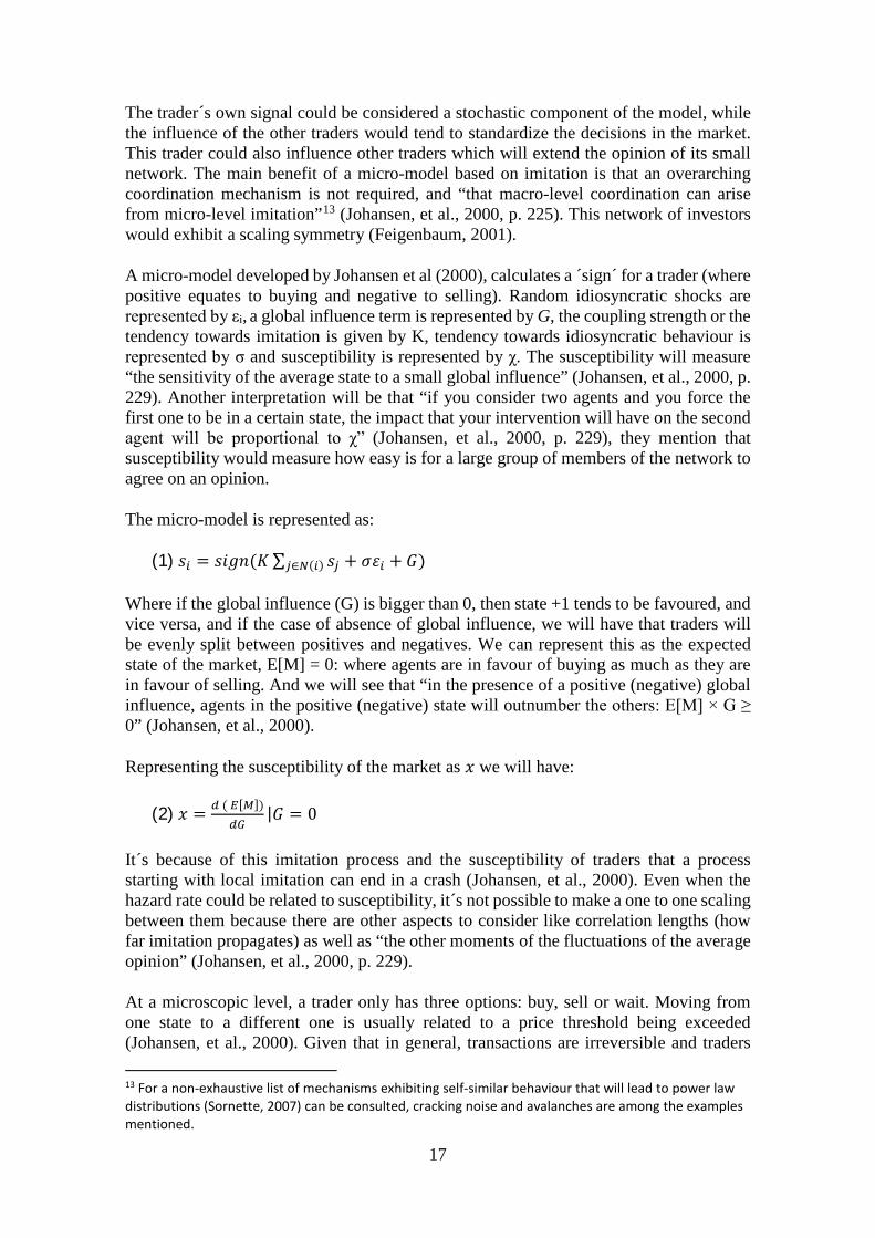
This trader will be influenced by 4 traders, but he will also produce his own idiosyncratic signal. He could still follow his own ´hunch´, but if the social pressure becomes too high, he will probably follow the majoritarian decision even if it goes against his own ideas.

17

The trader´s own signal could be considered a stochastic component of the model, while the influence of the other traders would tend to standardize the decisions in the market. This trader could also influence other traders which will extend the opinion of its small network. The main benefit of a micro-model based on imitation is that an overarching coordination mechanism is not required, and “that macro-level coordination can arise from micro-level imitation”13 (Johansen, et al., 2000, p. 225). This network of investors would exhibit a scaling symmetry (Feigenbaum, 2001).

A micro-model developed by Johansen et al (2000), calculates a ´sign´ for a trader (where positive equates to buying and negative to selling). Random idiosyncratic shocks are represented by εi, a global influence term is represented by G, the coupling strength or the tendency towards imitation is given by K, tendency towards idiosyncratic behaviour is represented by σ and susceptibility is represented by χ. The susceptibility will measure “the sensitivity of the average state to a small global influence” (Johansen, et al., 2000, p. 229). Another interpretation will be that “if you consider two agents and you force the first one to be in a certain state, the impact that your intervention will have on the second agent will be proportional to χ” (Johansen, et al., 2000, p. 229), they mention that susceptibility would measure how easy is for a large group of members of the network to agree on an opinion.

The micro-model is represented as:

(1) 𝑠𝑠𝑖𝑖 = 𝑠𝑠𝑠𝑠𝑔𝑔𝑠𝑠(𝐾𝐾∑ 𝑠𝑠𝑗𝑗 + 𝜎𝜎𝜀𝜀𝑖𝑖 + 𝐺𝐺)𝑗𝑗∈𝑁𝑁(𝑖𝑖)

Where if the global influence (G) is bigger than 0, then state +1 tends to be favoured, and vice versa, and if the case of absence of global influence, we will have that traders will be evenly split between positives and negatives. We can represent this as the expected state of the market, E[M] = 0: where agents are in favour of buying as much as they are in favour of selling. And we will see that “in the presence of a positive (negative) global influence, agents in the positive (negative) state will outnumber the others: E[M] × G ≥ 0” (Johansen, et al., 2000).

Representing the susceptibility of the market as 𝑥𝑥 we will have:

(2) 𝑥𝑥 = 𝑑𝑑 ( 𝐸𝐸[𝑀𝑀])𝑑𝑑𝑑𝑑

|𝐺𝐺 = 0

It´s because of this imitation process and the susceptibility of traders that a process starting with local imitation can end in a crash (Johansen, et al., 2000). Even when the hazard rate could be related to susceptibility, it´s not possible to make a one to one scaling between them because there are other aspects to consider like correlation lengths (how far imitation propagates) as well as “the other moments of the fluctuations of the average opinion” (Johansen, et al., 2000, p. 229).

At a microscopic level, a trader only has three options: buy, sell or wait. Moving from one state to a different one is usually related to a price threshold being exceeded (Johansen, et al., 2000). Given that in general, transactions are irreversible and traders 13 For a non-exhaustive list of mechanisms exhibiting self-similar behaviour that will lead to power law distributions (Sornette, 2007) can be consulted, cracking noise and avalanches are among the examples mentioned.

18

work based on limited information and can only see the cooperative responses to variations of price, it could be tempting to equate the stock market to other dynamical out-of-equilibrium systems, however we can´t forget that there´s a “reflectivity mechanism: the “microscopic” building blocks, the traders, are conscious of their actions.” (Johansen, et al., 2000, p. 219).

3.3) Price dynamics

Fundamental value investors buy/sell stocks when market values differ in significant amounts from the fundamental value of stocks. They will buy when the stock market price is lower that the fundamental value and sell when the opposite is true. That way they will mitigate crashes by buying stocks from those selling in panic (Barlevy & Veronesi, 2003)14.

Given that it´s not possible to calculate the fundamental value of a stock in a precise way (because every model needs inputs difficult to predict like interest rates and company growth15), forecast estimates could differ in great amounts. That´s why fundamental values are usually considered as a band, leading to low rotation of the portfolio of value investors, given that they will need a big movement in a stock price to make them take the decision to sell or buy a stock in their portfolio.

Trend followers will buy when they detect a rise in the price, causing a further rise. They will sell when they see falling prices, deepening crises. Noise traders think that they have information about the stock market, but they are only adding noise to the stock market, giving to the market its random motion component (Black, 1986). The hazard rate could be driven by the collective behaviour of noise traders.

This will be reflected on prices showing super-exponential acceleration and possibly “additional so-called ´log-periodic´ oscillations associated with a hierarchical organization and dynamics of noise traders” (Lin, et al., 2014, p. 210). Another dynamical explanation of the emergence of oscillatory patterns in prices considers “the competition between positive feedback (self-fulfilling sentiment), negative feedbacks (contrarian behaviour and fundamental value analysis) and inertia (everything takes time to adjust)” (Zhou & Sornette, 2009, p. 870). According to them, the competition between these market participants plus the effect of inertia would “lead to nonlinear oscillations approximating log-periodicity” (Zhou & Sornette, 2009, p. 870). Another point to have in mind, as to what provokes the log-periodic behaviour, is the fact that most investment strategies followed by trend followers are not linear “they tend to under-react for small price changes and over-react for large ones” (Ide & Sornette, 2002, p. 69).

The log-periodicity observed in the stock market before crashes has been interpreted as “the observable signature of the developing discrete hierarchy of alternating positive and negative feedbacks culminating in the final ´rupture´, which is the end of the bubble often associated with a crash” (Zhou & Sornette, 2009, p. 870). On the other hand, Feigenbaum

14 However (Barlevy & Veronesi, 2003) also observed a “shift from passive investing strategies to more aggressive trading practices such as day-trading” which could cause an amplification of the magnitude of crashes, if they were to occur. 15Even volatilities and the expected return on the market tend to change over time, and we don´t know if those changes are going to be abrupt or gradual (Black, 1986).

19

(2001, p. 2) mentions that log-periodicity in a physics environment is interpreted as “the signature of a spatial environment with a discrete scaling symmetry” and mentions that some studies have interpreted that log-periodicity patterns followed by crashes can be considered analogous to a physics interpretation of a critical point that corresponds with a phase transition.

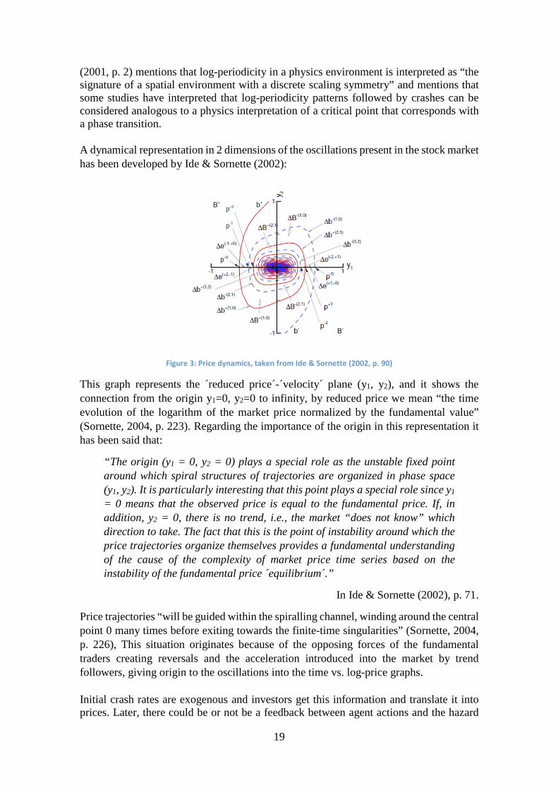
A dynamical representation in 2 dimensions of the oscillations present in the stock market has been developed by Ide & Sornette (2002):

Figure 3: Price dynamics, taken from Ide & Sornette (2002, p. 90)

This graph represents the ´reduced price´-´velocity´ plane (y1, y2), and it shows the connection from the origin y1=0, y2=0 to infinity, by reduced price we mean “the time evolution of the logarithm of the market price normalized by the fundamental value” (Sornette, 2004, p. 223). Regarding the importance of the origin in this representation it has been said that:

“The origin (y1 = 0, y2 = 0) plays a special role as the unstable fixed point around which spiral structures of trajectories are organized in phase space (y1, y2). It is particularly interesting that this point plays a special role since y1 = 0 means that the observed price is equal to the fundamental price. If, in addition, y2 = 0, there is no trend, i.e., the market “does not know” which direction to take. The fact that this is the point of instability around which the price trajectories organize themselves provides a fundamental understanding of the cause of the complexity of market price time series based on the instability of the fundamental price ´equilibrium´.”

In Ide & Sornette (2002), p. 71.

Price trajectories “will be guided within the spiralling channel, winding around the central point 0 many times before exiting towards the finite-time singularities” (Sornette, 2004, p. 226), This situation originates because of the opposing forces of the fundamental traders creating reversals and the acceleration introduced into the market by trend followers, giving origin to the oscillations into the time vs. log-price graphs.

Initial crash rates are exogenous and investors get this information and translate it into prices. Later, there could be or not be a feedback between agent actions and the hazard

20

rate. The crash itself is an exogenous event, even when everybody knows that it could be coming, nobody knows exactly why, so even when they can get compensated for it in the form of high prices, they can´t get abnormal returns (after adjusting by risk) by anticipating the crash (Johansen & Sornette, 2002). However, the specific way the market collapsed “is not the most important problem: a crash occurs because the market has entered an unstable phase and any small disturbance or process may have triggered the instability” (Sornette, 2003, p. 88). Once a system is unstable, many situations could have triggered the reaction (the crash), that´s why sometimes it is so difficult to find the exact origin of a crash and many different news could be pointed as the ´origin´ of the crisis, even when the real origin, was that the hazard rate was already high and the log-periodic price oscillations had no room to keep accelerating.

It has been suggested by Sornette & Johansen (1997, p. 420) that “the market anticipates the crash in a subtle self-organized and cooperative fashion, hence releasing precursory ´fingerprints´ observable in the stock market prices.” That is, they consider that there´s information to be picked up by investors from prices, however these subtle information has not been discovered by most.

Specific events can act as “revelators rather than the deep sources of the instability” (Johansen, et al., 1999, p. 20). Even political events can be considered revelators of the state of a bigger dynamical system in which the stock market is included. Endogenous crashes can be understood as “the natural deaths of self-organized self-reinforcing speculative bubbles giving rise to specific precursory signatures in the form of log-periodic power laws accelerating super-exponentially” (Johansen & Sornette, 2010, p. 5). However, there have been some exogenous crashes identified, in those cases, crashes can be related to some extraordinary events (Johansen & Sornette, 2010).

3.4) The LPPL Equation Originally, the equation designed to predict the critical time used the market index as a measure of the level of the market. However, to avoid getting distorted signals due to the exponential rise of price (and avoiding the need to de-trend, getting additional distortion), the logarithm of the index was preferred (Sornette & Johansen, 1997). Another advantage of this specification is due to investors being “primarily concerned with relative changes in stock prices rather than absolute changes” (Feigenbaum, 2001, p. 8).

Correct specification depends on the initial assumptions regarding the expected size of the crash, if we expect it to be proportional to the current price level, we would need to use the logarithm of the price (preferred for longer time scales like 8 years), however, if we expect the crash to be proportional to the amount earned during the bubble, the price itself should be used. This could be better suited for shorter time scales like two years (Johansen & Sornette, 1999).

The equation used in this document has been dubbed the “Linear” Log-Periodic Formula (even when it´s not really linear)16:

(3) log[𝑝𝑝(𝑡𝑡)] = 𝐴𝐴 + 𝐵𝐵(𝑡𝑡𝑐𝑐 − 𝑡𝑡)𝛽𝛽{1 + 𝐶𝐶 cos[𝜔𝜔 log(𝑡𝑡𝑐𝑐 − 𝑡𝑡) + 𝜙𝜙]}

16For a motivation and derivation of the formula we refer to (Sornette, 2004).

21

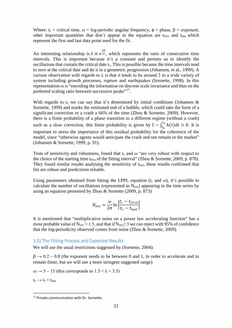
Where: tc = critical time, ω = log-periodic angular frequency, ϕ = phase, β = exponent, other important quantities that don´t appear in the equation are tfirst and tlast which represent the first and last data point used for the fit.

An interesting relationship is 𝜆𝜆 ≡ 𝑒𝑒2𝜋𝜋𝜔𝜔 , which represents the ratio of consecutive time

intervals. This is important because it´s a constant and permits us to identify the oscillations that contain the critical date tc. This is possible because the time intervals tend to zero at the critical date and do it in a geometric progression (Johansen, et al., 1999). A curious observation with regards to λ is that it tends to be around 2 in a wide variety of system including growth processes, rupture and earthquakes (Sornette, 1998). In this representation ω is “encoding the information on discrete scale invariance and thus on the preferred scaling ratio between successive peaks”17.

With regards to tc, we can say that it´s determined by initial conditions (Johansen & Sornette, 1999) and marks the estimated end of a bubble, which could take the form of a significant correction or a crash a 66% of the time (Zhou & Sornette, 2009). However, there is a finite probability of a phase transition to a different regime (without a crash) such as a slow correction, this finite probability is given by 1 − ∫ ℎ(𝑡𝑡)𝑑𝑑𝑡𝑡 > 0𝑡𝑡𝑐𝑐

𝑡𝑡0. It is

important to stress the importance of this residual probability for the coherence of the model, since “otherwise agents would anticipate the crash and not remain in the market” (Johansen & Sornette, 1999, p. 91).

Tests of sensitivity and robustness, found that tc and ω “are very robust with respect to the choice of the starting time tfirst of the fitting interval” (Zhou & Sornette, 2009, p. 878). They found similar results analysing the sensitivity of tlast, these results confirmed that fits are robust and predictions reliable.

Using parameters obtained from fitting the LPPL equation (tc and ω), it´s possible to calculate the number of oscillations (represented as Nosc) appearing in the time series by using an equation presented by Zhou & Sornette (2009, p. 873):

𝑁𝑁𝑜𝑜𝑜𝑜𝑐𝑐 =𝜔𝜔2𝜋𝜋

ln �𝑡𝑡𝑐𝑐 − 𝑡𝑡𝑓𝑓𝑖𝑖𝑓𝑓𝑜𝑜𝑡𝑡𝑡𝑡𝑐𝑐 − 𝑡𝑡𝑙𝑙𝑙𝑙𝑜𝑜𝑡𝑡

�

It is mentioned that “multiplicative noise on a power law accelerating function” has a most probable value of Nosc ≈ 1.5, and that if Nosc≥ 3 we can reject with 95% of confidence that the log-periodicity observed comes from noise (Zhou & Sornette, 2009).

3.5) The Fitting Process and Expected Results We will use the usual restrictions suggested by (Sornette, 2004):

β → 0.2 – 0.8 (the exponent needs to be between 0 and 1, in order to accelerate and to remain finite, but we will use a more stringent suggested range)

ω → 5 – 15 (this corresponds to 1.5 < λ < 3.5)

tc → tc > tlast

17 Private communication with Dr. Sornette.

22

ϕ → No restriction

After fitting the Portuguese stock market index to the LPPL equation, it could be expected to get reasonable fits with low errors as well as post-dictions of critical dates close to the real observed dates. However, it would be unrealistic to expect that the predicted tc coincides exactly with the time of the crash, because of the not fully deterministic nature of crashes (Johansen, et al., 2000). Another point considered by them is that false alarms could be unavoidable; but most endogenous crashes will be predicted. As a way to calculate the significance of the values for β and ω in the usual range, (Johansen & Sornette, 1999) analysed 400-week random intervals from 1910 to 1996 of the Dow Jones average and tried to fit the log-periodic equation. They only were able to find six data sets in the usual ranges, and all corresponded to periods previous to crashes: 1929, 1962 and 1987, these results strengthened the case for the reliability of this method of analysis.

Regarding the log-periodic angular frequency, a ´fundamental´ log periodic angular frequency has been identified in different analysis in the range ω1 ≈ 6.4 ± 1.5, other peaks having been found on its harmonics: ωn = nω1, however even when the importance of the harmonics are expected to decrease exponentially, ω2 and ω3 have been observed to be very significant, being this something more prevalent in individual stocks rather than in aggregate indexes because of the additional noise of the data (Zhou & Sornette, 2009).

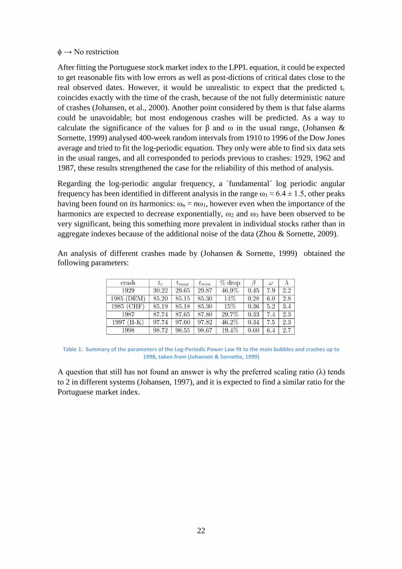
An analysis of different crashes made by (Johansen & Sornette, 1999) obtained the following parameters:

Table 1: Summary of the parameters of the Log-Periodic Power Law fit to the main bubbles and crashes up to 1998, taken from (Johansen & Sornette, 1999)

A question that still has not found an answer is why the preferred scaling ratio (λ) tends to 2 in different systems (Johansen, 1997), and it is expected to find a similar ratio for the Portuguese market index.

23

4) Contextual Analysis

As a way to provide some context to the Portuguese crashes of 1998, 2007 and 2015 that will be analysed in this document, the same timeframe in other markets is going to be reviewed.

4.1) 1997-1998 Crisis

An analysis of the 1997 East Asian crisis by (Radelet & Sachs, 1998) found its cause in the rapid forced liberalization of financial markets and the easy access to international credits without adequate supervision. It has been mentioned that the interventions by the IMF could not have helped to improve economic conditions, but by forcing the countries involved to more liberalizations it could have bolstered the increase of the credit bubble and attracted short term capital that only caused additional destabilization. Radelet & Sachs (1998, p. 71) see international financial markets as “inherently unstable, at least for countries borrowing heavily from abroad at short maturities and in foreign currency”. There were other examples of liberalizations led by the IMF in the same period that ended in macroeconomic crises.

Following the East Asian Crisis, the next important crisis was the 1998 Russian Crash which could have been “triggered by the Asian crises, but it was to a large extent fuelled by the collapse of a banking system, which in the course of the bubble had created an outstanding debt of $19.2 billion” (Johansen, et al., 1999, p. 21). These authors found “close to identical power law and log-periodic behaviour to the bubbles observed on Wall Street, the Hong-Kong stock market and on currencies”, showing how the parameters are similar in different markets around the world.

Regarding the United States, Feigenbaum (2001) found a log-periodic behaviour in 1997 and 1998 for the S&P 500 previous to the crash, and Johansen et al (2000) found an example of speculative bubble ending in a crash in the Nasdaq Composite in the 1997 – 2000 period, mentioning that the parameters obtained were in line with those obtained in different markets. Even when some analysts tried to link the 2000 Dot-com crash with an anti-trust issue involving Microsoft, Johansen et al (2000) consider that the stock market would have collapsed anyway.

4.2) 2007-2008 Crisis For a review of the Crash in the United States, we will borrow mainly from Krugman (2009) who made a recount of the events. The origin of the US crash based on the housing boom, however that bubble started to deflate since the fall of 2005, when demand started to decrease, even when the possibility to avoid down payments was present and having teaser-rate loans18 available. Given that house sellers are used to wait before houses get sold, they didn´t react immediately to the lack of demand, in fact, for a while prices kept going up despite the reduced sales.

18 Loans where the interest rate is very low at the beginning and increases after some years.

24

In the second quarter of 2006, the prices of houses started to go down slowly, and one year later, prices were just 3% down from the previous peak, however from that point to 2008, house prices went down 15 percent.

It is also important to mention that on July 19, 2007 the DJIA rose above 14,000 for the first time and two weeks later the White House released a self-congratulatory note, showing their optimism about the economic conditions in the United States, and while asked about the housing market problems on 1st August, Henry Paulson answered that those were largely contained, showing how it´s usually difficult for the experts on the field to predict a dramatic turn of events.

It is usually considered that August 9, 2007, the day the French bank BNP Paribas suspended withdrawals from three of its funds marked the beginning of a new financial crisis.

Back to the US, the reducing prices of houses allowed a new problem to arise: the fact that subprime lending had been approved in the basis of an ever growing house bubble, if that wouldn´t have been the case, borrowers could have just sold back the house when they wouldn´t afford the money for more payments or refinance, and the companies wouldn´t have lost money, however with shrinking prices borrowers ended with negative value equities19 and in many cases decided or were forced by their economic situation to stop the payments and lose the house, in those cases the lender could lose as much as 50% on the value of the loan.

Since many of those home loans were actually approved by a loan originator, then sold to a financial institution who sliced them and repackaged in different levels of seniority in order to sell them back to investors, many of those toxic debts (not only limited to subprime anymore, since the falling house prices led to many people with good credit records to default on their mortgage) ended in many different types of funds, even ones with conservative management, because the higher seniority tranches obtained an AAA rating.

When some funds tried to get rid of the Mortgage Backed Securities (MBS), it created a self-reinforcing process where funds tried to sell, increased volatilities and reduced prices, which originated additional margin requirements or the cut of credit lines, forcing the sale of additional securities (not limited at this point to MBS, since margin calls had to be met), since more and more types of assets were being sold in a rush in illiquid markets, the crisis extended to the market as a whole. An additional problem, was the weakening of the so-called shadow market, with some sectors of it totally disappearing and others being greatly reduced. In the end, despite the reduction of the Federal Funds Rate from 5.25% to 4.75% on September 18, 2007 and later reduction that let it in 0% since December 16, 2008, the crisis caused the rise of credit cards rates and higher credit costs for companies without top credit ratings.

4.3) 2015 Crisis China´s Stock Market reached a peak on June 12th, 2015, after years of upward movements and increasing fears of being in a bubble, market capitalization having

19 At 2009, there were 12 million home owners with negative equity in the US (Krugman, 2009)

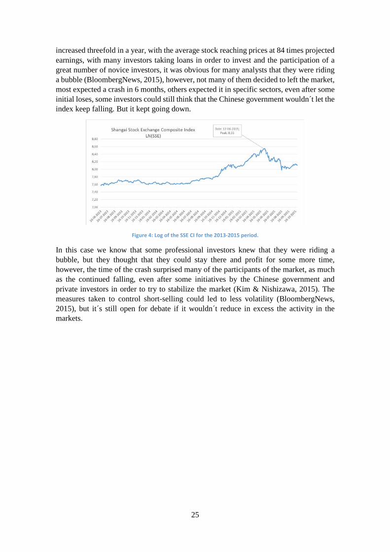
25

increased threefold in a year, with the average stock reaching prices at 84 times projected earnings, with many investors taking loans in order to invest and the participation of a great number of novice investors, it was obvious for many analysts that they were riding a bubble (BloombergNews, 2015), however, not many of them decided to left the market, most expected a crash in 6 months, others expected it in specific sectors, even after some initial loses, some investors could still think that the Chinese government wouldn´t let the index keep falling. But it kept going down.

Figure 4: Log of the SSE CI for the 2013-2015 period.

In this case we know that some professional investors knew that they were riding a bubble, but they thought that they could stay there and profit for some more time, however, the time of the crash surprised many of the participants of the market, as much as the continued falling, even after some initiatives by the Chinese government and private investors in order to try to stabilize the market (Kim & Nishizawa, 2015). The measures taken to control short-selling could led to less volatility (BloombergNews, 2015), but it´s still open for debate if it wouldn´t reduce in excess the activity in the markets.

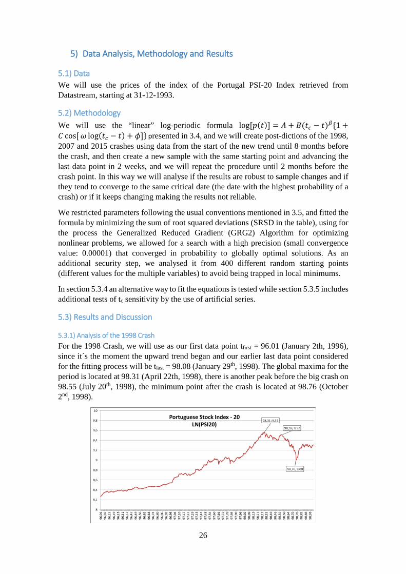
26

5) Data Analysis, Methodology and Results

5.1) Data We will use the prices of the index of the Portugal PSI-20 Index retrieved from Datastream, starting at 31-12-1993.

5.2) Methodology We will use the “linear” log-periodic formula log[𝑝𝑝(𝑡𝑡)] = 𝐴𝐴 + 𝐵𝐵(𝑡𝑡𝑐𝑐 − 𝑡𝑡)𝛽𝛽{1 +𝐶𝐶 cos[𝜔𝜔 log(𝑡𝑡𝑐𝑐 − 𝑡𝑡) + 𝜙𝜙]} presented in 3.4, and we will create post-dictions of the 1998, 2007 and 2015 crashes using data from the start of the new trend until 8 months before the crash, and then create a new sample with the same starting point and advancing the last data point in 2 weeks, and we will repeat the procedure until 2 months before the crash point. In this way we will analyse if the results are robust to sample changes and if they tend to converge to the same critical date (the date with the highest probability of a crash) or if it keeps changing making the results not reliable.

We restricted parameters following the usual conventions mentioned in 3.5, and fitted the formula by minimizing the sum of root squared deviations (SRSD in the table), using for the process the Generalized Reduced Gradient (GRG2) Algorithm for optimizing nonlinear problems, we allowed for a search with a high precision (small convergence value: 0.00001) that converged in probability to globally optimal solutions. As an additional security step, we analysed it from 400 different random starting points (different values for the multiple variables) to avoid being trapped in local minimums.

In section 5.3.4 an alternative way to fit the equations is tested while section 5.3.5 includes additional tests of tc sensitivity by the use of artificial series.

5.3) Results and Discussion

5.3.1) Analysis of the 1998 Crash For the 1998 Crash, we will use as our first data point tfirst = 96.01 (January 2th, 1996), since it´s the moment the upward trend began and our earlier last data point considered for the fitting process will be tlast = 98.08 (January 29th, 1998). The global maxima for the period is located at 98.31 (April 22th, 1998), there is another peak before the big crash on 98.55 (July 20th, 1998), the minimum point after the crash is located at 98.76 (October 2nd, 1998).

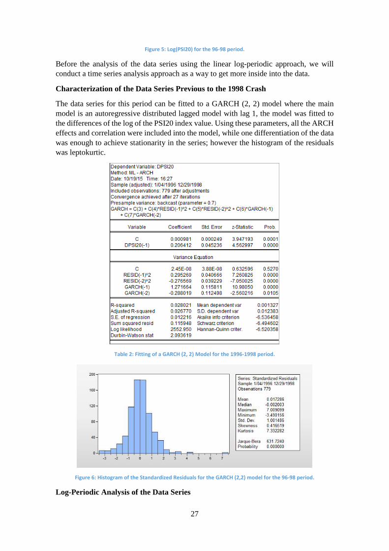
27

Figure 5: Log(PSI20) for the 96-98 period.

Before the analysis of the data series using the linear log-periodic approach, we will conduct a time series analysis approach as a way to get more inside into the data.

Characterization of the Data Series Previous to the 1998 Crash

The data series for this period can be fitted to a GARCH (2, 2) model where the main model is an autoregressive distributed lagged model with lag 1, the model was fitted to the differences of the log of the PSI20 index value. Using these parameters, all the ARCH effects and correlation were included into the model, while one differentiation of the data was enough to achieve stationarity in the series; however the histogram of the residuals was leptokurtic.

Table 2: Fitting of a GARCH (2, 2) Model for the 1996-1998 period.

Figure 6: Histogram of the Standardized Residuals for the GARCH (2,2) model for the 96-98 period.

Log-Periodic Analysis of the Data Series

28

In the table we will present the results of all the minimization process, where SRSD is the sum of root squared deviations, NDP is the number of data points, tlast is the last data point. In all cases the analysis started in 96.01 (02-01-1996). Highlighted in the table is the post-diction realized 3 months before the lowest point, which means that the tlast was 98.50 (the lowest data point in the period was 98.75, and there was a tenuous local peak at 98.55).

Table 3: Fitting of the Log-Periodic “Linear” Model for the 1996-1998 period for samples with different ending points (tlast).

We can observe that when our analysis have samples ending from 98.08 to 98.17 the critical time is calculated as 98.18 well before the time of the crash (and almost immediately after the last data point), that seems to be an usual occurrence, it seems as if the log-periodic fit is coupling to some structure in the data that doesn´t represent the complete series. A similar situation can be observed when the last data point is 98.21. However a totally different result is obtained when the last data point is between 98.25 and 98.50, when the critical time starts being predicted at a period between 99.64 and 98.70 (the lowest data point is at 98.75), which is consistent with the fact that usually the predicted critical point is before the real data of the crash. For samples ending in 98.54 and 98.59, we end again in a situation where the critical time is predicted immediately after the last data point.

Considering that the lowest level of the stock market was in 98.75, we would have been able to prevent with some anticipation of the upcoming crash, considering that we were able to get reasonable predictions while restricting the parameters to the conventional ranges for the method used (namely β between 0.2 to 0.8 and ω between 5 and 15). The value of λ ranged from 1.52 to 2.35, showing values around 2, as expected.

As an additional point, we can mention that Nosc > 3, which would show with 95% of confidence that the log-periodic oscillations are not coming from noise, we will see similar results regarding oscillations in the following two tables.

96 A B C β φ tc ω λ SRSD SRSD / NDP tlast tlast natural Nosc NDP1 9,41 -0,68 0,14 0,51 199,91 98,18 7,35 2,35 12,57 0,02 98,08 29-01-1998 3,60 5422 9,41 -0,68 0,14 0,51 199,91 98,18 7,35 2,35 12,74 0,02 98,12 13-02-1998 4,23 5533 9,41 -0,69 0,14 0,51 199,91 98,18 7,42 2,33 12,88 0,02 98,17 02-03-1998 6,05 5644 9,69 -0,93 0,09 0,42 199,42 98,28 8,91 2,02 13,53 0,02 98,21 17-03-1998 4,84 5755 11,78 -2,86 -0,02 0,20 74,86 98,64 14,09 1,56 13,69 0,02 98,25 01-04-1998 4,27 5866 11,79 -2,86 -0,02 0,20 74,91 98,64 13,96 1,57 14,09 0,02 98,29 16-04-1998 4,49 5977 10,94 -1,99 0,03 0,30 109,37 98,66 15,00 1,52 14,83 0,02 98,33 01-05-1998 4,95 6088 10,94 -1,99 0,03 0,30 109,36 98,66 15,00 1,52 15,36 0,02 98,38 18-05-1998 5,33 6199 10,87 -1,92 0,03 0,30 109,35 98,66 15,00 1,52 16,12 0,03 98,42 02-06-1998 5,70 63010 10,61 -1,65 0,04 0,35 109,26 98,68 15,00 1,52 17,93 0,03 98,46 17-06-1998 5,97 64111 10,57 -1,60 0,04 0,36 109,13 98,70 15,00 1,52 20,63 0,03 98,50 02-07-1998 6,21 65212 9,61 -0,71 -0,08 0,74 194,99 98,55 15,00 1,52 22,95 0,03 98,54 17-07-1998 12,93 66313 9,61 -0,68 -0,08 0,77 194,77 98,60 15,00 1,52 24,27 0,04 98,59 03-08-1998 13,05 674

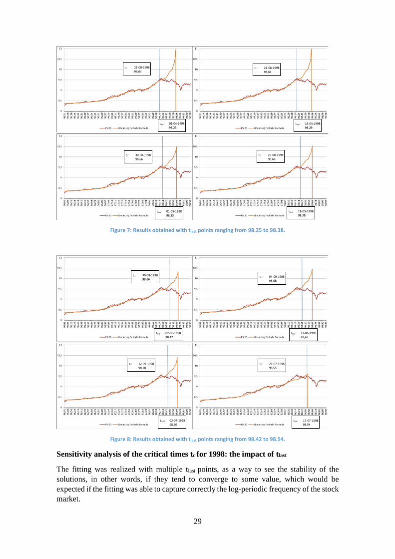
29

Figure 7: Results obtained with tlast points ranging from 98.25 to 98.38.

Figure 8: Results obtained with tlast points ranging from 98.42 to 98.54.

Sensitivity analysis of the critical times tc for 1998: the impact of tlast

The fitting was realized with multiple tlast points, as a way to see the stability of the solutions, in other words, if they tend to converge to some value, which would be expected if the fitting was able to capture correctly the log-periodic frequency of the stock market.

tlast: 02-06-1998 98,42

tc: 30-08-1998 98,66

tlast: 17-06-1998 98,46

tc: 04-09-1998 98,68

tlast: 02-07-1998 98,50

tc: 12-09-1998 98,70

tlast: 17-07-1998 98,54

tc: 21-07-1998 98,55

tlast: 01-04-1998 98,25

tc: 21-08-1998 98,64

tlast: 16-04-1998 98,29

tc: 21-08-1998 98,64

tlast: 01-05-1998 98,33

tc: 30-08-1998 98,66

tlast: 18-05-1998 98,38

tc: 29-08-1998 98,66

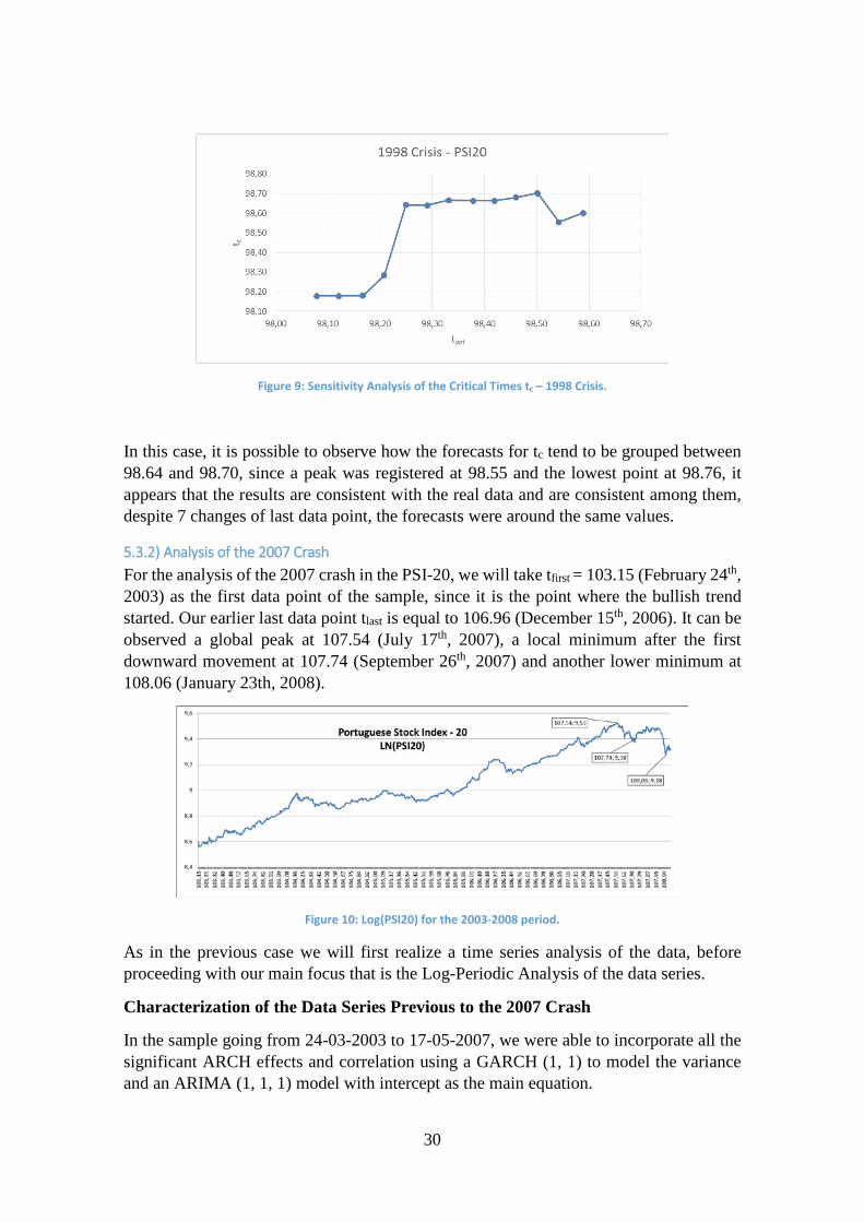
30

Figure 9: Sensitivity Analysis of the Critical Times tc – 1998 Crisis.

In this case, it is possible to observe how the forecasts for tc tend to be grouped between 98.64 and 98.70, since a peak was registered at 98.55 and the lowest point at 98.76, it appears that the results are consistent with the real data and are consistent among them, despite 7 changes of last data point, the forecasts were around the same values.

5.3.2) Analysis of the 2007 Crash For the analysis of the 2007 crash in the PSI-20, we will take tfirst = 103.15 (February 24th, 2003) as the first data point of the sample, since it is the point where the bullish trend started. Our earlier last data point tlast is equal to 106.96 (December 15th, 2006). It can be observed a global peak at 107.54 (July 17th, 2007), a local minimum after the first downward movement at 107.74 (September 26th, 2007) and another lower minimum at 108.06 (January 23th, 2008).

Figure 10: Log(PSI20) for the 2003-2008 period.

As in the previous case we will first realize a time series analysis of the data, before proceeding with our main focus that is the Log-Periodic Analysis of the data series.

Characterization of the Data Series Previous to the 2007 Crash

In the sample going from 24-03-2003 to 17-05-2007, we were able to incorporate all the significant ARCH effects and correlation using a GARCH (1, 1) to model the variance and an ARIMA (1, 1, 1) model with intercept as the main equation.

31

Table 4: Fitting of a GARCH (1, 1) Model for the 2003-2007 period.

As in the previous analysis our residuals are leptokurtic:

Figure 11: Histogram of the Standardized Residuals for the GARCH (1, 1) model for the 2003-2007 period.

Log-Periodic Analysis of the Data Series

In the case of the 2007 crash, we will mention that the peak before the crash was registered at 107.54, while the lowest point was registered at 108.06. Highlighted in the table the situation where the last data point is 3 months before the peak, at 107.29.

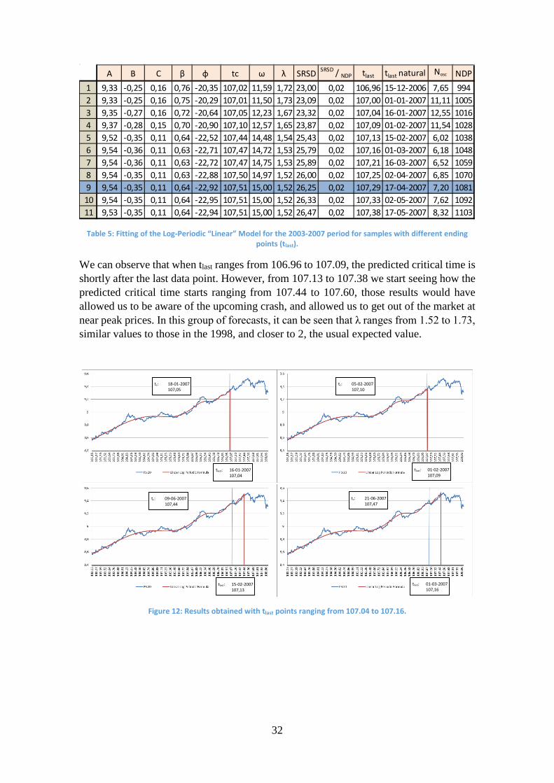
32

Table 5: Fitting of the Log-Periodic “Linear” Model for the 2003-2007 period for samples with different ending points (tlast).

We can observe that when tlast ranges from 106.96 to 107.09, the predicted critical time is shortly after the last data point. However, from 107.13 to 107.38 we start seeing how the predicted critical time starts ranging from 107.44 to 107.60, those results would have allowed us to be aware of the upcoming crash, and allowed us to get out of the market at near peak prices. In this group of forecasts, it can be seen that λ ranges from 1.52 to 1.73, similar values to those in the 1998, and closer to 2, the usual expected value.

Figure 12: Results obtained with tlast points ranging from 107.04 to 107.16.

103 A B C β φ tc ω λ SRSD SRSD / NDP tlast tlast natural Nosc NDP1 9,33 -0,25 0,16 0,76 -20,35 107,02 11,59 1,72 23,00 0,02 106,96 15-12-2006 7,65 9942 9,33 -0,25 0,16 0,75 -20,29 107,01 11,50 1,73 23,09 0,02 107,00 01-01-2007 11,11 10053 9,35 -0,27 0,16 0,72 -20,64 107,05 12,23 1,67 23,32 0,02 107,04 16-01-2007 12,55 10164 9,37 -0,28 0,15 0,70 -20,90 107,10 12,57 1,65 23,87 0,02 107,09 01-02-2007 11,54 10285 9,52 -0,35 0,11 0,64 -22,52 107,44 14,48 1,54 25,43 0,02 107,13 15-02-2007 6,02 10386 9,54 -0,36 0,11 0,63 -22,71 107,47 14,72 1,53 25,79 0,02 107,16 01-03-2007 6,18 10487 9,54 -0,36 0,11 0,63 -22,72 107,47 14,75 1,53 25,89 0,02 107,21 16-03-2007 6,52 10598 9,54 -0,35 0,11 0,63 -22,88 107,50 14,97 1,52 26,00 0,02 107,25 02-04-2007 6,85 10709 9,54 -0,35 0,11 0,64 -22,92 107,51 15,00 1,52 26,25 0,02 107,29 17-04-2007 7,20 108110 9,54 -0,35 0,11 0,64 -22,95 107,51 15,00 1,52 26,33 0,02 107,33 02-05-2007 7,62 109211 9,53 -0,35 0,11 0,64 -22,94 107,51 15,00 1,52 26,47 0,02 107,38 17-05-2007 8,32 1103

tlast: 16-01-2007 107,04

tc: 18-01-2007 107,05

tlast: 01-02-2007 107,09

tc: 05-02-2007 107,10

tlast: 15-02-2007 107,13

tc: 09-06-2007 107,44

tlast: 01-03-2007 107,16

tc: 21-06-2007 107,47

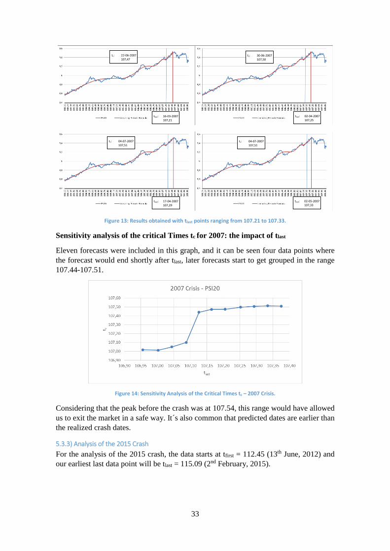
33

Figure 13: Results obtained with tlast points ranging from 107.21 to 107.33.

Sensitivity analysis of the critical Times tc for 2007: the impact of tlast

Eleven forecasts were included in this graph, and it can be seen four data points where the forecast would end shortly after tlast, later forecasts start to get grouped in the range 107.44-107.51.

Figure 14: Sensitivity Analysis of the Critical Times tc – 2007 Crisis.

Considering that the peak before the crash was at 107.54, this range would have allowed us to exit the market in a safe way. It´s also common that predicted dates are earlier than the realized crash dates.

5.3.3) Analysis of the 2015 Crash For the analysis of the 2015 crash, the data starts at tfirst = 112.45 (13th June, 2012) and our earliest last data point will be tlast = 115.09 (2nd February, 2015).

tlast: 02-05-2007 107,33

tc: 04-07-2007 107,51

tc: 22-06-2007 107,47

tlast: 16-03-2007 107,21

tlast: 02-04-2007 107,25

tc: 30-06-2007 107,50

tc: 04-07-2007 107,51

tlast: 17-04-2007 107,29

34

Figure 15: Log(PSI20) for the 2012-2015 period.

In this graph, the attention is going to be concentred in the data after 115.09, that way it can be observed the existence of local valleys at 115.02 (January 7th, 2015), 115.52 (July 7th, 2015) and 115.65 (August 24th, 2015), while there are local peaks at 115.27 (April 9th, 2015) and 115.54 (July 14th, 2015). Later the peaks and valleys from the real data will be compared with the results obtained from the LPPL fit.

Characterization of the Data Series Previous to the 2015 Crash

We fitted an Autoregressive Distributed Lag Model with one lag to remove correlation and one level of differentiation to remove stationarity, an intercept was not included for not being statistically significant. The modelling of the variance was a GARCH (2, 2) that removed all the significant ARCH effects from the data.

Table 6: Fitting of a GARCH (2, 2), using an Auto Regressive Distributed Lag Model with one lag and no intercept as the main equation for the 2012-2015 period.

As in the previous two cases, the residuals also showed excessive kurtosis:

35

Figure 16: Histogram of the Standardized Residuals for the GARCH (2, 2) model for the 2012-2015 period.

Log-Periodic Analysis of the Data Series

The 2014-2015 period is interesting because it shows different peak points, where we get critical times not long after the last data point (but not immediately after either). There´s a local maximum in the stock market at 115.30 (25th April, 2015), and the lowest point after that peak is achieved at 115.65 (24th August, 2015).

Table 7: Fitting of the Log-Periodic “Linear” Model for the 2012-2015 period for samples with different ending

points (tlast).

When the last data point ranges from 115.09 to 115.25, the critical time goes from 115.20 to 115.29, around the local peak at 115.30, while when the last data point is around 3 months before the lowest data point, but after the local peak (115.42 and 115.46), the critical time is indicated as 115.65, the point of the lowest data point.

In this group of tests, λ ranges from 1.91 to 3.31, and the Nosc is greater than three starting with tc=115.28.

112 A B C β φ tc ω λ SRSD SRSD / NDP tlast tlast natural Nosc NDP1 8,37 0,31 0,56 0,20 31,84 115,20 5,64 3,05 34,15 0,05 115,09 02-02-2015 2,88 6852 8,37 0,31 0,55 0,20 31,67 115,25 5,92 2,89 34,61 0,05 115,13 16-02-2015 2,99 6953 8,37 0,31 0,55 0,20 31,54 115,28 6,19 2,76 34,90 0,05 115,17 02-03-2015 3,13 7054 8,40 0,28 0,60 0,25 0,17 115,28 6,23 2,74 35,05 0,05 115,21 16-03-2015 3,63 7155 8,63 0,01 -21,10 0,23 53,27 115,29 5,25 3,31 36,56 0,05 115,25 02-04-2015 3,57 7286 8,30 0,39 0,40 0,20 -13,07 115,47 8,41 2,11 36,86 0,05 115,29 16-04-2015 3,81 7367 8,65 0,01 -20,07 0,23 52,95 115,39 6,10 2,80 37,54 0,05 115,34 04-05-2015 3,95 7478 8,42 0,26 0,57 0,20 -13,45 115,54 8,53 2,09 37,86 0,05 115,38 18-05-2015 4,03 7579 8,42 0,27 0,53 0,20 30,04 115,65 9,72 1,91 38,77 0,05 115,42 02-06-2015 4,09 76810 8,45 0,24 0,59 0,20 -13,96 115,65 9,55 1,93 39,31 0,05 115,46 16-06-2015 4,29 77811 8,66 0,01 -19,07 0,27 52,50 115,51 7,21 2,39 40,29 0,05 115,50 02-07-2015 6,70 790

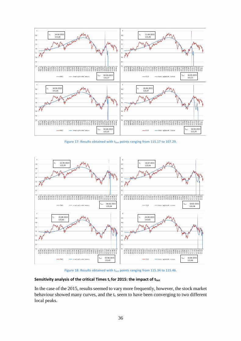
36

Figure 17: Results obtained with tlast points ranging from 115.17 to 107.29.

Figure 18: Results obtained with tlast points ranging from 115.34 to 115.46.

Sensitivity analysis of the critical Times tc for 2015: the impact of tlast

In the case of the 2015, results seemed to vary more frequently, however, the stock market behaviour showed many curves, and the tc seem to have been converging to two different local peaks.

tlast: 02-03-2015 115,17

tc: 14-04-2015 115,28

tlast: 16-03-2015 115,21

tc: 11-04-2015 115,28

tlast: 02-04-2015 115,25

tc: 16-04-2015 115,29

tlast: 16-04-2015 115,29

tc: 18-06-2015 115,47

tlast: 04-05-2015 115,34

tc: 22-05-2015 115,39

tlast: 18-05-2015 115,38

tc: 14-07-2015 115,54

tlast: 02-06-2015 115,42

tc: 23-08-2015 115,65

tlast: 16-06-2015 115,46

tc: 24-08-2015 115,65

37

Figure 19: Sensitivity Analysis of the Critical Times tc – 2015 Crisis.

Considering that the peak at 115.27 is not a global maximum, it´s possible that the bubble had already started to get deflated and make the fits not so stable. An analysis considering a sample ending before the global peak in the 2012-2015 period could be done, however, in this case, it was intended to include as much information as possible, to see how good the fits were adjusted to the latest real data.

5.3.4) Log-Periodic Analysis of the Data minimizing the Root Mean Squared Deviation In the previous optimization processes we obtained the best fit by minimizing the sum of the root of the squared deviations between the log linear model and the log of the data, however the Root Mean Squared deviation measure requires the minimization of the root of the sum of the squared differences divided by the number of data points:

Where 𝑦𝑦𝑡𝑡� are the predicted values, y are the market values and n are the number of data points included in the sample. In this case, the number to minimize is going to be normalized around zero (and not around some random number, dependent on the number of data points), however, the results of both processes must be similar and equivalent20.

To test this approach, we will realize the minimization procedure in three selected data points, for the stock market in 1998, 2007 and 2015, the tlast selected being 98.50, 107.29 and 115.42.

20 Private communication with Prof. António Da Ascensão Costa.

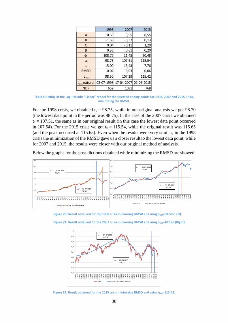
38

Table 8: Fitting of the Log-Periodic “Linear” Model for the selected ending points for 1998, 2007 and 2015 Crisis,

minimizing the RMSD.

For the 1998 crisis, we obtained tc = 98.75, while in our original analysis we got 98.70 (the lowest data point in the period was 98.75). In the case of the 2007 crisis we obtained tc = 107.51, the same as in our original result (in this case the lowest data point occurred in 107.54). For the 2015 crisis we got tc = 115.54, while the original result was 115.65 (and the peak occurred at 115.65). Even when the results were very similar, in the 1998 crisis the minimization of the RMSD gave us a closer result to the lowest data point, while for 2007 and 2015, the results were closer with our original method of analysis.

Below the graphs for the post-dictions obtained while minimizing the RMSD are showed:

Figure 20: Result obtained for the 1998 crisis minimizing RMSD and using tlast=98.50 (Left).

Figure 21: Result obtained for the 2007 crisis minimizing RMSD and using tlast=107.29 (Right).

Figure 22: Result obtained for the 2015 crisis minimizing RMSD and using tlast=115.42.

1998 2007 2015A 10,58 9,55 8,55B -1,58 -0,37 0,13C 0,04 -0,11 1,20β 0,36 0,61 0,20φ 108,75 11,45 30,48tc 98,75 107,51 115,54ω 15,00 15,43 7,76

RMSD 0,04 0,03 0,06tlast 98,50 107,29 115,42

tlast natural 02-07-1998 17-04-2007 02-06-2015NDP 652 1081 768

tc: 29-09-1998 98,75

tlast: 02-07-1998 98,50

tc: 05-07-1998 107,51

tc: 17-04-2007 107,29

tlast: 02-06-2015 115,42

tc: 14-07-2015 115,54

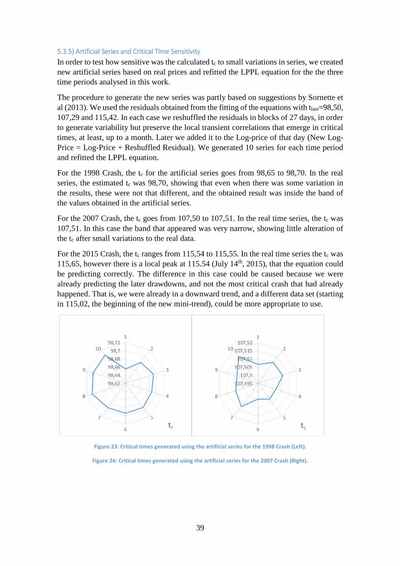
39

5.3.5) Artificial Series and Critical Time Sensitivity In order to test how sensitive was the calculated tc to small variations in series, we created new artificial series based on real prices and refitted the LPPL equation for the the three time periods analysed in this work.

The procedure to generate the new series was partly based on suggestions by Sornette et al (2013). We used the residuals obtained from the fitting of the equations with tlast=98,50, 107,29 and 115,42. In each case we reshuffled the residuals in blocks of 27 days, in order to generate variability but preserve the local transient correlations that emerge in critical times, at least, up to a month. Later we added it to the Log-price of that day (New Log-Price = Log-Price + Reshuffled Residual). We generated 10 series for each time period and refitted the LPPL equation.

For the 1998 Crash, the tc for the artificial series goes from 98,65 to 98,70. In the real series, the estimated tc was 98,70, showing that even when there was some variation in the results, these were not that different, and the obtained result was inside the band of the values obtained in the artificial series.

For the 2007 Crash, the tc goes from 107,50 to 107,51. In the real time series, the tc was 107,51. In this case the band that appeared was very narrow, showing little alteration of the tc after small variations to the real data.

For the 2015 Crash, the tc ranges from 115,54 to 115,55. In the real time series the tc was 115,65, however there is a local peak at 115.54 (July 14th, 2015), that the equation could be predicting correctly. The difference in this case could be caused because we were already predicting the later drawdowns, and not the most critical crash that had already happened. That is, we were already in a downward trend, and a different data set (starting in 115,02, the beginning of the new mini-trend), could be more appropriate to use.

Figure 23: Critical times generated using the artificial series for the 1998 Crash (Left).

Figure 24: Critical times generated using the artificial series for the 2007 Crash (Right).

40

Figure 25: Critical times generated using the artificial series for the 2015 Crash.

In this case, this was a test for demonstrative purposes, but we think that by using a high number of artificial series, we could be able to construct a band around the expected critical time, helping us to be able to be better prepared for upcoming crashes by having some margin of manoeuvre and getting to know a full range of dates with increased risk and not only the most critical point.

41

6) Conclusions, Recommendations, Limitations and Future Research

6.1) Main Conclusions The methodology exposed here would have allowed us to avoid big loses in the 1998 Portuguese crash and would have permitted us to sell at points near the peak in the 2007 crash, in the case of the 2015 crisis, we would have obtained a good indication of the moment were the lowest data point was going to be achieved.

Predictions of critical time appear to be stable regarding the last data point included. In those cases, if we get a string of values of tc surrounding some specific number and we have seen the number of oscillations required to verify that the log-periodicity is not coming from noise (Nosc = 3), we would have to take into consideration the results coming from the model.

Parameter values have been in line with those observed in other markets, which means that the formulas also work for Portugal, even when this is a small market and the index considered is only composed of 20 stocks.

Regarding the fitting procedure, the minimization of SRSD or RMSD seem to be equally good. About the use of artificial series, those could provide a way to measure how stable are our critical time predictions relative to small perturbations, and to generate bands that could be expected to land around the real critical time.

6.2) Recommendations The use of this methodology could be helpful in order to prevent major losses in diversified stocks portfolios, whenever we are at a bubble situation. Given that Log-Periodic Analysis can also be applied to the GNP, a joint analysis could be done.

In case of applying this technique to individual stocks, it´s necessary to remember that the series are going to be much noisier, and it could be necessary to allow more freedom for the parameters to achieve a good fit.

6.3) Limitations and Future Research The fitting procedures using artificial time series were limited since those were used for testing purposes, however in order to get a high reliability, we would need to use a high number of artificial series.

Another test to be done, is related to the sensitivity of forecastings to the initial time tfirst, also analysis in individual stocks in the Portuguese stock market could be performed. The analysis of anti-bubbles is not attempted here, however there is analysis to be done especially in the 2003-2008 period.

Analysis using the so-called ´Nonlinear´ log-periodic formula, can also be tried. A more comprehensive study of the statistical measure to be minimized in order to obtain better fits can also be performed.

42

References Barlevy, G. & Veronesi, P., 2003. Rational panics and stock market crashes. Journal of Economic

Theory, 110(2), pp. 234-263.

Bastiaensen, K., Cauwels, P., Sornette, D. & Woodard, R. & Zhou, W.-X., 2009. The Chinese Equity Bubble :Ready to Burst.[Online] Available at: http://arxiv.org/abs/0907.1827

Black, F., 1986. Noise. The Journal of Finance, XLI(3), pp. 529-543.

Blanchard, O. J., 1979. Speculative bubbles, crashes and rational expectations. Economics Letters , Volumen 3, pp. 387-389.

BloombergNews, 2015. Crash, No Escape for China Hedge Funds Overwhelmed by Stocks. Bloomberg Business, 15 September.

BloombergNews, 2015. The China Bubble Is Going to Burst. Bloomberg Business, 16 June.

Blume, M. E. & Siegel, J., 1992. The Theory of Security Pricing and Market Structure 1: 3-57.. Financial Markets, Institutions and Instruments , Volume 1, pp. 3-57.

Crutchfield, J. P., 2009. The Hidden Fragility of Complex Systems: Consequences of Change, Changing Consequences, s.l.: Santa Fe Institute.

Devenow, A. & Welch, I., 1996. Rational herding in financial economics. European Economic Review, Issue 40, pp. 603-615.

Eguiluz, V. M. & Zimmermann, M. G., 2000. Transmission of Information and Herd Behavior: an Application to Financial Markets. Physical Review Letters, Volumen 85, pp. 5659-5662.

Fama, E., 1965. Random Walks in Stock Market Prices. Selected Papers of the Graduate School of Business, University of Chicago, Issue 16.

Farmer, J. D., Patelli, P. & Zovko, I. I., 2005. The predictive power of zero intelligence in financial markets. Proceedings of the National Academy of Sciences of the United States of America, 102(6), p. 2254–2259.

Feigenbaum, J., 2001. A Statistical Analysis of Log-Periodic Precursors to Financial Crashes. [Online] Available at: arXiv:cond-mat/0101031v2

Gode, D. K. & Sunder, S., 1993. Allocative Efficiency of Markets with Zero-Intelligence Traders: Market as a Partial Substitute for Individual Rationality. Journal of Political Economy, 101(1), pp. 119-137.

Graham, J. R., 1999. Herding Among Investment Newsletters: Theory and Evidence. The Journal of Finance, LIV(1), pp. 237-268.

Granovetter, M., 1978. Threshold Models of Collective Behavior. The American Journal of Sociology, 83(6), pp. 1420-1443.

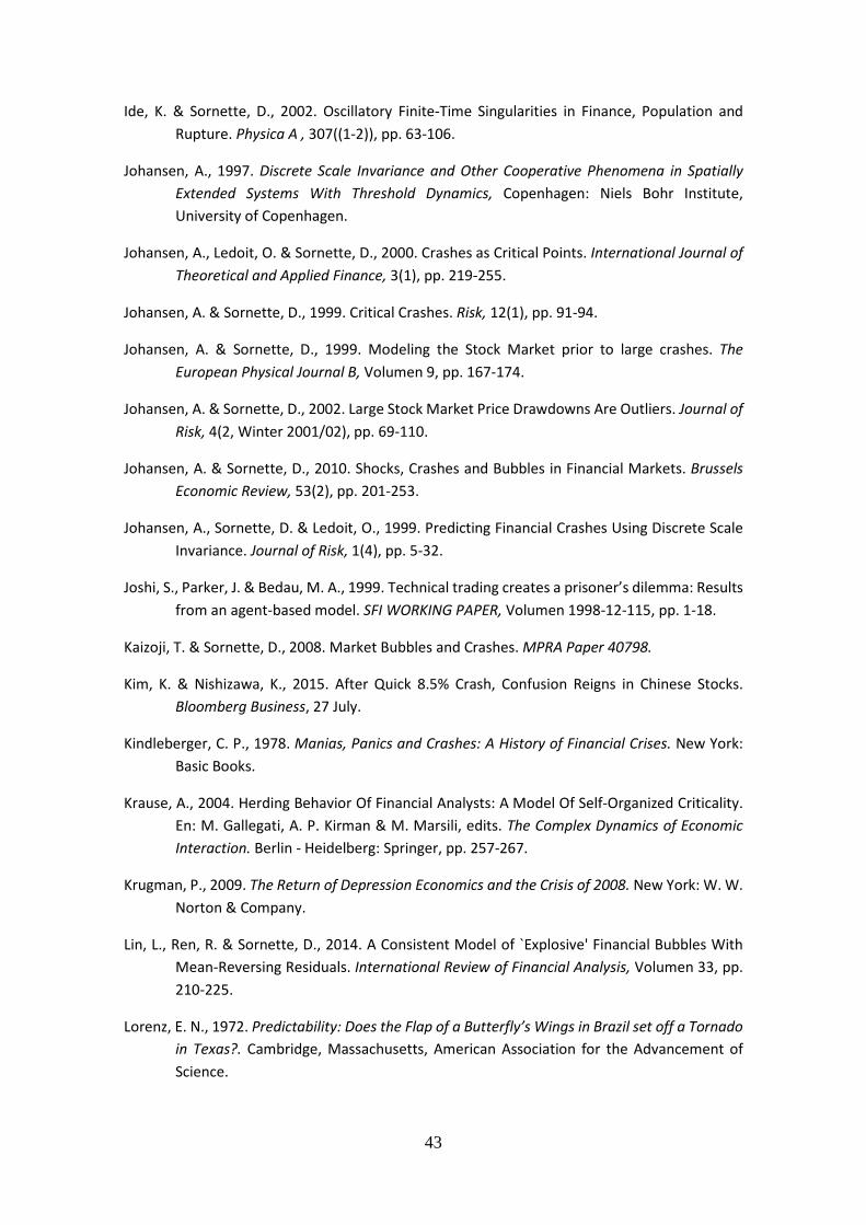
43

Ide, K. & Sornette, D., 2002. Oscillatory Finite-Time Singularities in Finance, Population and Rupture. Physica A , 307((1-2)), pp. 63-106.

Johansen, A., 1997. Discrete Scale Invariance and Other Cooperative Phenomena in Spatially Extended Systems With Threshold Dynamics, Copenhagen: Niels Bohr Institute, University of Copenhagen.

Johansen, A., Ledoit, O. & Sornette, D., 2000. Crashes as Critical Points. International Journal of Theoretical and Applied Finance, 3(1), pp. 219-255.

Johansen, A. & Sornette, D., 1999. Critical Crashes. Risk, 12(1), pp. 91-94.

Johansen, A. & Sornette, D., 1999. Modeling the Stock Market prior to large crashes. The European Physical Journal B, Volumen 9, pp. 167-174.

Johansen, A. & Sornette, D., 2002. Large Stock Market Price Drawdowns Are Outliers. Journal of Risk, 4(2, Winter 2001/02), pp. 69-110.

Johansen, A. & Sornette, D., 2010. Shocks, Crashes and Bubbles in Financial Markets. Brussels Economic Review, 53(2), pp. 201-253.

Johansen, A., Sornette, D. & Ledoit, O., 1999. Predicting Financial Crashes Using Discrete Scale Invariance. Journal of Risk, 1(4), pp. 5-32.

Joshi, S., Parker, J. & Bedau, M. A., 1999. Technical trading creates a prisoner’s dilemma: Results from an agent-based model. SFI WORKING PAPER, Volumen 1998-12-115, pp. 1-18.

Kaizoji, T. & Sornette, D., 2008. Market Bubbles and Crashes. MPRA Paper 40798.

Kim, K. & Nishizawa, K., 2015. After Quick 8.5% Crash, Confusion Reigns in Chinese Stocks. Bloomberg Business, 27 July.

Kindleberger, C. P., 1978. Manias, Panics and Crashes: A History of Financial Crises. New York: Basic Books.

Krause, A., 2004. Herding Behavior Of Financial Analysts: A Model Of Self-Organized Criticality. En: M. Gallegati, A. P. Kirman & M. Marsili, edits. The Complex Dynamics of Economic Interaction. Berlin - Heidelberg: Springer, pp. 257-267.

Krugman, P., 2009. The Return of Depression Economics and the Crisis of 2008. New York: W. W. Norton & Company.

Lin, L., Ren, R. & Sornette, D., 2014. A Consistent Model of `Explosive' Financial Bubbles With Mean-Reversing Residuals. International Review of Financial Analysis, Volumen 33, pp. 210-225.

Lorenz, E. N., 1972. Predictability: Does the Flap of a Butterfly’s Wings in Brazil set off a Tornado in Texas?. Cambridge, Massachusetts, American Association for the Advancement of Science.

44

Malkiel, B. G., 2003. The Efficient Market Hypothesis and Its Critics. Journal of Economic Perspectives, 17(1), pp. 59-82.

Orlean, A., 1989. Mimetic Contagion and Speculative Bubbles. Theory and Decision, Volumen 27, pp. 63-92.

Radelet, S. & Sachs, J. D., 1998. The East Asian Financial Crisis: Diagnosis, Remedies, Prospects. Brookings Papers on Economic Activity, 29(1), pp. 1-90.

Romer, D., 1993. Rational Asset-Price Movements Without News. The American Economic Review, 83(5), pp. 1112-1130.

Rubinstein, M., 2000. Rational Markets: Yes or No? The Affirmative Case, California: Research Program in Finance Working Papers.

Sornette, D., 1998. Discrete scale invariance and complex dimensions. Physics Reports, Volumen 297, pp. 239-270.

Sornette, D., 2002. Predictability of catastrophic events: material rupture, earthquakes, turbulence, financial crashes and human birth. Proceedings of the National Academy of Sciences, 99(SUPP1), pp. 2522-2529 .

Sornette, D., 2003. Critical market crashes. Physics Reports, Volume 378, pp. 1-98.

Sornette, D., 2004. Why Stock Markets Crash? Critical Events in Complex Financial Systems. Fifth Printing and First Paperback Printing ed. New Jersey: Princeton University Press.

Sornette, D., 2007. Probability Distributions in Complex Systems. In: Encyclopedia of Complexity and System Science. New York: Springer Science, pp. 7009-7024.

Sornette, D. & Andersen, J., 2002. A Nonlinear Super-Exponential Rational Model of Speculative Financial Bubbles. International Journal of Modern Physics C, 13(2), pp. 171-188.

Sornette, D. & Cauwels, P., 2014. 1980–2008: The Illusion of the Perpetual Money Machine and What It Bodes for the Future. Risks, 2(2), pp. 103-131.

Sornette, D. & Johansen, A., 1997. Large financial crashes. Physica A, Volumen 245, pp. 411-422.

Sornette, D. & Johansen, A., 2001. Significance of log-periodic precursors to financial crashes. Quantitative Finance, 1(4), pp. 452-471.

Sornette, D., Woodard, R., Yan, W. & Zhou, W.-X., 2013. Clarifications to questions and criticisms on the Johansen–Ledoit–Sornette financial bubble model. Physica A, Volumen 392, p. 4417–4428.

Thompson, E. A., 2006. The tulipmania: Fact or artifact?. Public Choice, 130(1-2), pp. 99-114.

Thompson, J. R. & Wilson, J. R., 2013. Multifractal Analysis of Agent-Bases Financial Markets. Washington, IEEE.

45

Timmermann, A. & Granger, C. W. J., 2004. Efficient market hypothesis and forecasting. International Journal of Forecasting, Volumen 20, p. 15– 27.

Tryfos,P.,2001. Are Stock Prices Predictable?. [Online] Available at: http://www.yorku.ca/ptryfos/busstats.htm [Accessed 4 11 2014].

Weites, B. & Maravic, M. v., 2010. How To Detect Bubbles in Stock Prices? Econometric bubble detection – A survey and new tests, Aarhus: Aarhus School of Business and Social Sciences, Aarhus University.

Yan, W., Woodard, R. & Sornette, D., 2011. Diagnosis and Prediction of Market Rebounds in Financial Markets. [Online] Available at: http://arxiv.org/abs/1003.5926

Youssefmir, M., Huberman, B. A. & Tad, H., 1998. Bubbles and Market Crashes. Computational Economics, Volume 12, pp. 97-114.

Zhou, W.-X. & Sornette, D., 2009. A case study of speculative financial bubbles in the South African stock market 2003–2006. Physica A: Statistical Mechanics and its Applications, 388(6), pp. 869-880.

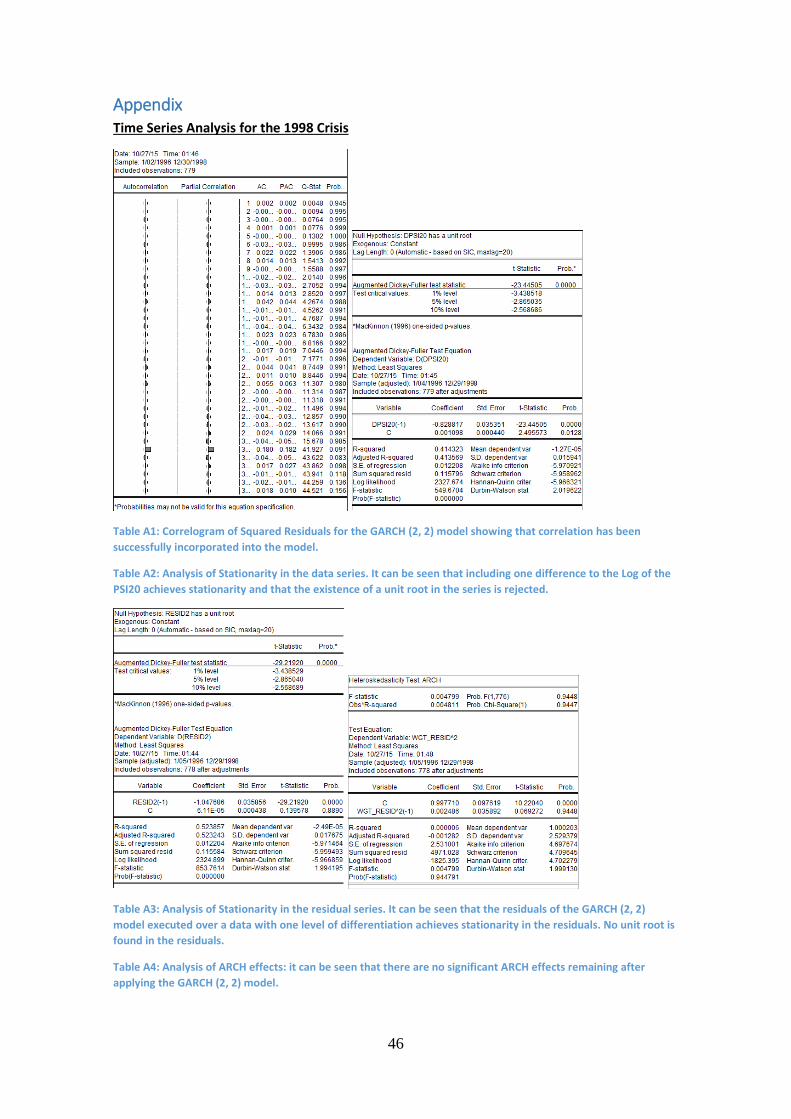
46

Appendix Time Series Analysis for the 1998 Crisis

Table A1: Correlogram of Squared Residuals for the GARCH (2, 2) model showing that correlation has been successfully incorporated into the model.

Table A2: Analysis of Stationarity in the data series. It can be seen that including one difference to the Log of the PSI20 achieves stationarity and that the existence of a unit root in the series is rejected.

Table A3: Analysis of Stationarity in the residual series. It can be seen that the residuals of the GARCH (2, 2) model executed over a data with one level of differentiation achieves stationarity in the residuals. No unit root is found in the residuals.

Table A4: Analysis of ARCH effects: it can be seen that there are no significant ARCH effects remaining after applying the GARCH (2, 2) model.

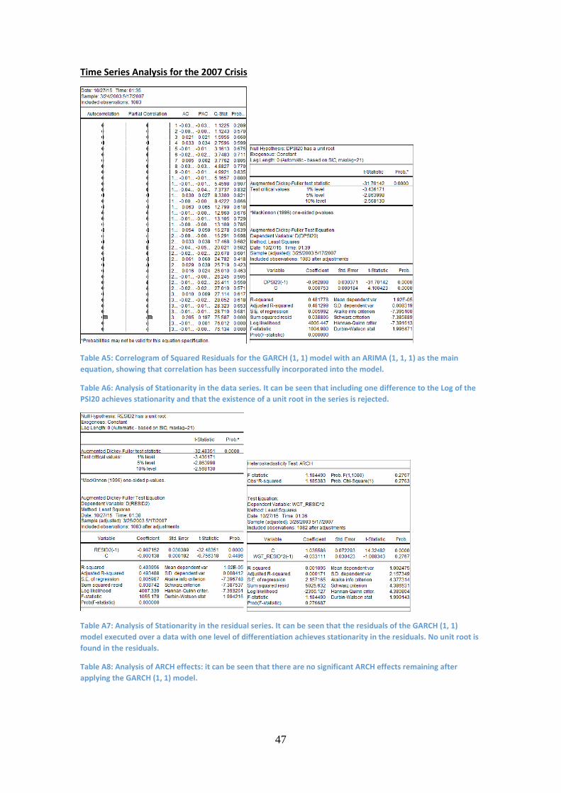
47

Time Series Analysis for the 2007 Crisis

Table A5: Correlogram of Squared Residuals for the GARCH (1, 1) model with an ARIMA (1, 1, 1) as the main equation, showing that correlation has been successfully incorporated into the model.

Table A6: Analysis of Stationarity in the data series. It can be seen that including one difference to the Log of the PSI20 achieves stationarity and that the existence of a unit root in the series is rejected.

Table A7: Analysis of Stationarity in the residual series. It can be seen that the residuals of the GARCH (1, 1) model executed over a data with one level of differentiation achieves stationarity in the residuals. No unit root is found in the residuals.

Table A8: Analysis of ARCH effects: it can be seen that there are no significant ARCH effects remaining after applying the GARCH (1, 1) model.

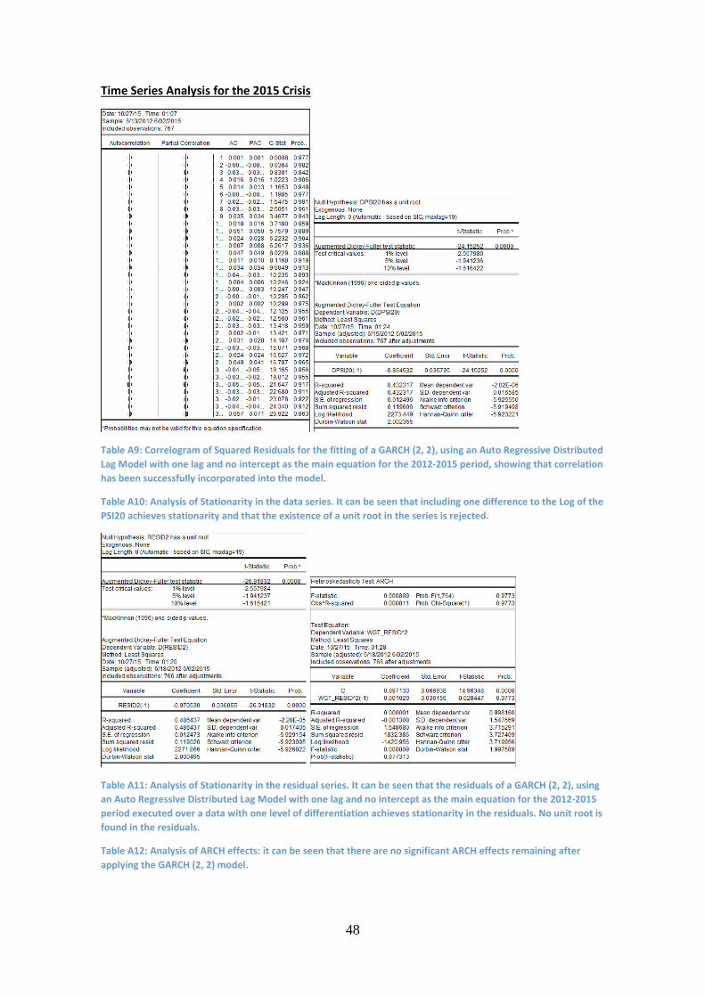
48

Time Series Analysis for the 2015 Crisis

Table A9: Correlogram of Squared Residuals for the fitting of a GARCH (2, 2), using an Auto Regressive Distributed Lag Model with one lag and no intercept as the main equation for the 2012-2015 period, showing that correlation has been successfully incorporated into the model.

Table A10: Analysis of Stationarity in the data series. It can be seen that including one difference to the Log of the PSI20 achieves stationarity and that the existence of a unit root in the series is rejected.

Table A11: Analysis of Stationarity in the residual series. It can be seen that the residuals of a GARCH (2, 2), using an Auto Regressive Distributed Lag Model with one lag and no intercept as the main equation for the 2012-2015 period executed over a data with one level of differentiation achieves stationarity in the residuals. No unit root is found in the residuals.

Table A12: Analysis of ARCH effects: it can be seen that there are no significant ARCH effects remaining after applying the GARCH (2, 2) model.