9/Maio/2018 – Aula 17

14/Maio/2018 – Aula 18

18 Ondas mecânicas 18.1 Tipos de ondas 18.2 Ondas periódicas 18.3 Descrição matemática

17 Movimentos oscilatórios, amortecidos e forçados 17.1 Movimento na vertical 17.2 Pêndulo simples 17.3 Pêndulo físico 17.4 Oscilações amortecidas 17.5 Oscilações forçadas

1

Quando um objeto se encontra pendurado na extremidade de uma mola vertical, fica sujeito ao seu peso, para além da força de restituição da mola.

2

17.1 Movimento oscilatório na vertical

y ' = y − y0

Fy = −k y +mg∑ = 0

Se o sistema estiver em equilíbrio:

Se se deslocar o sistema ligeiramente para fora do equilíbrio:

d2y '

dt2= −kmy '

y ' = Acos ωt +δ( ) , ω=km

U =12k y '( )2 +U0

Aula anterior

The path of the point mass (sometimes called a pendulum bob) is not a straightline but the arc of a circle with radius L equal to the length of the string (Fig. 14.21b). We use as our coordinate the distance x measured along the arc. Ifthe motion is simple harmonic, the restoring force must be directly proportionalto x or (because to Is it?

In Fig. 14.21b we represent the forces on the mass in terms of tangential andradial components. The restoring force is the tangential component of the netforce:

(14.30)

The restoring force is provided by gravity; the tension T merely acts to make thepoint mass move in an arc. The restoring force is proportional not to but to

so the motion is not simple harmonic. However, if the angle is small,is very nearly equal to in radians (Fig. 14.22). For example, when rad(about a difference of only 0.2%. With this approximation,Eq. (14.30) becomes

or

(14.31)

The restoring force is then proportional to the coordinate for small displace-ments, and the force constant is From Eq. (14.10) the angular fre-quency of a simple pendulum with small amplitude is

(14.32)

The corresponding frequency and period relationships are

(14.33)

(14.34)

Note that these expressions do not involve the mass of the particle. This isbecause the restoring force, a component of the particle’s weight, is proportionalto m. Thus the mass appears on both sides of and cancels out. (This is thesame physics that explains why bodies of different masses fall with the sameacceleration in a vacuum.) For small oscillations, the period of a pendulum for agiven value of g is determined entirely by its length.

The dependence on L and g in Eqs. (14.32) through (14.34) is just what weshould expect. A long pendulum has a longer period than a shorter one. Increas-ing g increases the restoring force, causing the frequency to increase and theperiod to decrease.

We emphasize again that the motion of a pendulum is only approximately sim-ple harmonic. When the amplitude is not small, the departures from simple har-monic motion can be substantial. But how small is “small”? The period can beexpressed by an infinite series; when the maximum angular displacement is the period T is given by

(14.35)

We can compute the period to any desired degree of precision by taking enoughterms in the series. We invite you to check that when (on either side of™ = 15°

T = 2pALga1 + 12

22 sin2 ™2

+ 12 # 32

22 # 42 sin4 ™2

+ Áb™,

©FS

! maS

T = 2pv

= 1ƒ

= 2pALg (simple pendulum, small amplitude)

ƒ = v

2p= 1

2p A gL (simple pendulum, small amplitude)

(simple pendulum,small amplitude)v = A k

m= Bmg>L

m= A g

L

vk = mg>L.

Fu = -mgL

x

Fu = -mgu = -mgxL

sinu = 0.0998,6°),u = 0.1u

sinuusinu,u

Fu = -mg sinu

Fu

u.x = Lu)

454 CHAPTER 14 Periodic Motion

The restoring force on thebob is proportional to sin u,not to u. However, for smallu, sin u ^ u, so the motion isapproximately simple harmonic.

Bob is modeledas a point mass.

(a) A real pendulum

(b) An idealized simple pendulum

L

T

x

mg sin u

mg

mg cos u

m

u

u

String isassumed to bemassless andunstretchable.

14.21 The dynamics of a simple pendulum.

2p/2 2p/4 p/4 p/2 u (rad)

FuFu 5 2mg sin u(actual)Fu 5 2mgu(approximate)

22mg

2mg

mg

2mg

O

14.22 For small angular displacementsthe restoring force on a

simple pendulum is approximately equalto that is, it is approximately pro-portional to the displacement Hence forsmall angles the oscillations are simpleharmonic.

u.-mgu;

Fu = -mg sinuu,

Na aproximação dos ângulos pequenos, , tem-se

3

17.2 Pêndulo simples

Nestas condições, a força de restituição é proporcional ao deslocamento, pelo que

F = −mg senθ ≈ −mgθ = −mg xL

senθ ≈θ

ω=km=mg Lm

=gL

T = 2πω

= 2π mk= 2π L

g

Note-se que o período T não depende da massa m do pêndulo.

Pêndulo vs M.Mola

simulação

Aula anterior

L senθ

θL

4

17.3 Pêndulo físico

O pêndulo físico consiste num objeto que pode rodar em torno de um eixo que não passa pelo centro de massa.

No exemplo da figura, o momento da força gravítica, em relação ao eixo de rotação, é

τ = −LsenθMg ≈ −LθMg(na aproximação dos ângulos pequenos)

O período de oscilação depende do momento de inércia I e da distância L entre o eixo de rotação e o centro de massa:

T = 2π IMg L

Aula anterior

5

17.4 Oscilações amortecidas

Na maior parte dos sistemas físicos reais, existem forças não-conservativas que tendem a dissipar a energia. No caso dos movimentos oscilatórios, a presença dessas forças é visível na diminuição da amplitude das oscilações. Por exemplo, no caso de atrito viscoso, essas forças (ditas de arrastamento), são proporcionais à velocidade:

Então, a força total sobre o objeto será a soma da força de restituição com a força de arrastamento:

!D = −b !v

!F = −k

!x −b

!v = −k

!x −b d

!xdt

d2!x

dt2= −km!x − bmd!xdt

Aula anterior

The angular frequency of oscillation is given by

(14.43)

You can verify that Eq. (14.42) is a solution of Eq. (14.41) by calculating the firstand second derivatives of x, substituting them into Eq. (14.41), and checkingwhether the left and right sides are equal. This is a straightforward but slightlytedious procedure.

The motion described by Eq. (14.42) differs from the undamped case in twoways. First, the amplitude is not constant but decreases with timebecause of the decreasing exponential factor Figure 14.26 is a graph ofEq. (14.42) for the case it shows that the larger the value of b, the morequickly the amplitude decreases.

Second, the angular frequency given by Eq. (14.43), is no longer equal tobut is somewhat smaller. It becomes zero when b becomes so large that

(14.44)

When Eq. (14.44) is satisfied, the condition is called critical damping. The sys-tem no longer oscillates but returns to its equilibrium position without oscillationwhen it is displaced and released.

If b is greater than the condition is called overdamping. Again thereis no oscillation, but the system returns to equilibrium more slowly than with crit-ical damping. For the overdamped case the solutions of Eq. (14.41) have the form

where and are constants that depend on the initial conditions and and are constants determined by m, k, and b.

When b is less than the critical value, as in Eq. (14.42), the condition is calledunderdamping. The system oscillates with steadily decreasing amplitude.

In a vibrating tuning fork or guitar string, it is usually desirable to have as littledamping as possible. By contrast, damping plays a beneficial role in the oscillationsof an automobile’s suspension system. The shock absorbers provide a velocity-dependent damping force so that when the car goes over a bump, it doesn’t continuebouncing forever (Fig. 14.27). For optimal passenger comfort, the system should becritically damped or slightly underdamped. Too much damping would be counter-productive; if the suspension is overdamped and the car hits a second bump justafter the first one, the springs in the suspension will still be compressed somewhatfrom the first bump and will not be able to fully absorb the impact.

Energy in Damped OscillationsIn damped oscillations the damping force is nonconservative; the mechanicalenergy of the system is not constant but decreases continuously, approachingzero after a long time. To derive an expression for the rate of change of energy,we first write an expression for the total mechanical energy E at any instant:

To find the rate of change of this quantity, we take its time derivative:

But and so

dEdt

= vx1max + kx2dx>dt = vx,dvx>dt = ax

dEdt

= mvxdvx

dt+ kx

dxdt

E = 12 mvx

2 + 12 kx2

a2a1C2C1

x = C1e-a1t + C2e-a2t

21km ,

km

- b2

4m2 = 0 or b = 21km

v = 2k>m v¿,

f = 0;e-1b>2m2t.Ae-1b>2m2t

v¿ = B km

- b2

4m2 (oscillator with little damping)

v¿

458 CHAPTER 14 Periodic Motion

O

2A

A

T0 2T0 3T0 4T0 5T0

Ae2(b/2m)t

xb ! 0.1!km (weak damping force)b ! 0.4!km (stronger damping force)

With stronger damping (larger b):• The amplitude (shown by the dashed curves) decreases more rapidly.• The period T increases (T0 ! period with zero damping).

t

14.26 Graph of displacement versustime for an oscillator with little damping[see Eq. (14.42)] and with phase angle

The curves are for two values ofthe damping constant b.f = 0.

Piston

Viscousfluid

Lower cylinderattached toaxle; moves upand down.

Pushed up

Pushed down

Upper cylinderattached to car’sframe; moves little.

14.27 An automobile shock absorber.The viscous fluid causes a damping forcethat depends on the relative velocity of thetwo ends of the unit.

6

17.4 Oscilações amortecidas

x = A0 exp −b2mt

⎛

⎝⎜

⎞

⎠⎟ cos ω 't +δ( )

A amplitude das oscilações diminui exponencialmente com o tempo:

M.Mola amortecida

simulação

E = E0 exp −bmt

⎛

⎝⎜

⎞

⎠⎟

e a energia mecânica (total) também:

Aula anterior

7

17.5 Oscilações forçadas

Para se manter um sistema amortecido em oscilação, é necessário forçar o movimento, imprimindo uma força exterior, no sentido do movimento. Essa força deve oscilar com uma frequência próxima da frequência própria do sistema (ω0):

ω0 =km

ω0 =gL

Então, a força total sobre o objeto será a soma da força de restituição com a força de arrastamento, com a força que obriga a que o movimento se mantenha:

!F = −k

!x −b d

!xdt

+ F0 cosωt

!Fext =

!F0 cosωt

Aula anterior

8

A=F0

m2 ω02 −ω2( )

2+b2ω2

17.5 Oscilações forçadas

Na ressonância, a frequência de oscilação é igual (ou muito próxima) da frequência própria do sistema: ω = ω0

Tacoma Bridge

filme

In November, 1940, the newly completed Tacoma Narrows Bridge, opened barely four months before, swayed and collapsed in a 42 mile-per-hour wind.

Aula anterior

9

18. Ondas

Uma perturbação (ou oscilação) que se desloque no espaço é uma onda. As ondas que necessitam de um suporte material (meio) para se deslocarem são ondas mecânicas.

10

18.1 Tipos de ondas

Ondas transversais: o deslocamento do meio é perpendicular à direção de propagação. Ondas longitudinais: o deslocamento do meio é paralelo à direção de propagação.

15.1 Types of Mechanical Waves 473

15.1 Types of Mechanical WavesA mechanical wave is a disturbance that travels through some material or sub-stance called the medium for the wave. As the wave travels through the medium,the particles that make up the medium undergo displacements of various kinds,depending on the nature of the wave.

Figure 15.1 shows three varieties of mechanical waves. In Fig. 15.1a themedium is a string or rope under tension. If we give the left end a small upwardshake or wiggle, the wiggle travels along the length of the string. Successivesections of string go through the same motion that we gave to the end, but at suc-cessively later times. Because the displacements of the medium are perpendicularor transverse to the direction of travel of the wave along the medium, this iscalled a transverse wave.

In Fig. 15.1b the medium is a liquid or gas in a tube with a rigid wall at theright end and a movable piston at the left end. If we give the piston a singleback-and-forth motion, displacement and pressure fluctuations travel down thelength of the medium. This time the motions of the particles of the medium are backand forth along the same direction that the wave travels. We call this alongitudinal wave.

In Fig. 15.1c the medium is a liquid in a channel, such as water in an irrigationditch or canal. When we move the flat board at the left end forward and backonce, a wave disturbance travels down the length of the channel. In this case thedisplacements of the water have both longitudinal and transverse components.

Each of these systems has an equilibrium state. For the stretched string it is thestate in which the system is at rest, stretched out along a straight line. For thefluid in a tube it is a state in which the fluid is at rest with uniform pressure. Andfor the liquid in a trough it is a smooth, level water surface. In each case the wavemotion is a disturbance from the equilibrium state that travels from one region ofthe medium to another. And in each case there are forces that tend to restore thesystem to its equilibrium position when it is displaced, just as the force of gravitytends to pull a pendulum toward its straight-down equilibrium position when it isdisplaced.

Motion of the waveParticles of the string

Particles of the fluid

Surface particles of the liquid

v

v

v

v

v

vAs the wave passes, eachparticle of the string moves upand then down, transversely tothe motion of the wave itself.

As the wave passes, eachparticle of the fluid movesforward and then back, parallelto the motion of the wave itself.

As the wave passes, eachparticle of the liquid surfacemoves in a circle.

(a) Transverse wave on a string

(b) Longitudinal wave in a fluid

(c) Waves on the surface of a liquid

15.1 Three ways to make a wave that moves to the right. (a) The hand moves the string up and then returns, producing atransverse wave. (b) The piston moves to the right, compressing the gas or liquid, and then returns, producing a longitudinalwave. (c) The board moves to the right and then returns, producing a combination of longitudinal and transverse waves.

Application Waves on a Snake’s BodyA snake moves itself along the ground by producing waves that travel backward along its body from its head to its tail. Thewaves remain stationary with respect to theground as they push against the ground, sothe snake moves forward.

ActivPhysics 10.1: Properties of MechanicalWaves

11

18.1 Tipos de ondas

v

v

v

Ondas contínuas:

Impulsos:

“Pacotes” de impulsos:

12

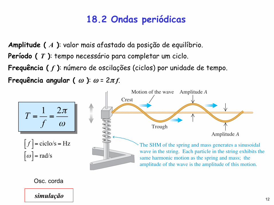
Amplitude ( A ): valor mais afastado da posição de equilíbrio. Período ( T ): tempo necessário para completar um ciclo. Frequência ( f ): número de oscilações (ciclos) por unidade de tempo.

Frequência angular ( ω ): ω = 2π f.

T = 1f=2πω

f⎡⎣ ⎤⎦= ciclo/s = Hz

ω⎡⎣ ⎤⎦= rad/s

These examples have three things in common. First, in each case the distur-bance travels or propagates with a definite speed through the medium. This speedis called the speed of propagation, or simply the wave speed. Its value is deter-mined in each case by the mechanical properties of the medium. We will use thesymbol for wave speed. (The wave speed is not the same as the speed withwhich particles move when they are disturbed by the wave. We’ll return to thispoint in Section 15.3.) Second, the medium itself does not travel through space;its individual particles undergo back-and-forth or up-and-down motions aroundtheir equilibrium positions. The overall pattern of the wave disturbance is whattravels. Third, to set any of these systems into motion, we have to put in energyby doing mechanical work on the system. The wave motion transports thisenergy from one region of the medium to another. Waves transport energy, butnot matter, from one region to another (Fig. 15.2).

v

474 CHAPTER 15 Mechanical Waves

15.2 “Doing the wave” at a sports stadium is an example of a mechanicalwave: The disturbance propagates throughthe crowd, but there is no transport of matter (none of the spectators moves from one seat to another).

Test Your Understanding of Section 15.1 What type of wave is “the wave”shown in Fig. 15.2? (i) transverse; (ii) longitudinal; (iii) a combination of transverse andlongitudinal. ❙

15.2 Periodic WavesThe transverse wave on a stretched string in Fig. 15.1a is an example of a wavepulse. The hand shakes the string up and down just once, exerting a transverseforce on it as it does so. The result is a single “wiggle,” or pulse, that travelsalong the length of the string. The tension in the string restores its straight-lineshape once the pulse has passed.

A more interesting situation develops when we give the free end of the stringa repetitive, or periodic, motion. (You may want to review the discussion ofperiodic motion in Chapter 14 before going ahead.) Then each particle in thestring also undergoes periodic motion as the wave propagates, and we have aperiodic wave.

Periodic Transverse WavesIn particular, suppose we move the string up and down with simple harmonicmotion (SHM) with amplitude A, frequency angular frequency andperiod Figure 15.3 shows one way to do this. The wave thatresults is a symmetrical sequence of crests and troughs. As we will see, periodic

T = 1>ƒ = 2p>v.v = 2pƒ,ƒ,

The SHM of the spring and mass generates a sinusoidalwave in the string. Each particle in the string exhibits thesame harmonic motion as the spring and mass; theamplitude of the wave is the amplitude of this motion.

Crest

Trough

Amplitude AMotion of the wave

Amplitude A

15.3 A block of mass m attached to a spring undergoes simple harmonic motion, pro-ducing a sinusoidal wave that travels to the right on the string. (In a real-life system adriving force would have to be applied to the block to replace the energy carried away bythe wave.)

18.2 Ondas periódicas

Osc. corda

simulação

15.2 Periodic Waves 475

t 5 0

T18t 5

T28t 5

T38t 5

T48t 5

T58t 5

T68t 5

T78t 5

Tt 5

Three points on the stringOscillatorgenerating wave

The wave advancesby one wavelength lduring each period T.

Each point moves up and down inplace. Particles one wavelength apartmove in phase with each other.

x

y

x

y

x

y

x

y

x

y

x

y

x

y

x

y

x

y

l

The string is shown at time intervals of periodfor a total of one period T. The highlightingshows the motion of one wavelength of the wave.

18

15.4 A sinusoidal transverse wave trav-eling to the right along a string. The verti-cal scale is exaggerated.

l

15.5 A series of drops falling into waterproduces a periodic wave that spreadsradially outward. The wave crests andtroughs are concentric circles. The wave-length is the radial distance betweenadjacent crests or adjacent troughs.

l

waves with simple harmonic motion are particularly easy to analyze; we call themsinusoidal waves. It also turns out that any periodic wave can be represented as acombination of sinusoidal waves. So this particular kind of wave motion is worthspecial attention.

In Fig. 15.3 the wave that advances along the string is a continuous succes-sion of transverse sinusoidal disturbances. Figure 15.4 shows the shape of a partof the string near the left end at time intervals of of a period, for a total time ofone period. The wave shape advances steadily toward the right, as indicated bythe highlighted area. As the wave moves, any point on the string (any of the reddots, for example) oscillates up and down about its equilibrium position withsimple harmonic motion. When a sinusoidal wave passes through a medium,every particle in the medium undergoes simple harmonic motion with the samefrequency.

CAUTION Wave motion vs. particle motion Be very careful to distinguish between themotion of the transverse wave along the string and the motion of a particle of the string.The wave moves with constant speed along the length of the string, while the motionof the particle is simple harmonic and transverse (perpendicular) to the length of thestring. ❙

For a periodic wave, the shape of the string at any instant is a repeating pat-tern. The length of one complete wave pattern is the distance from one crest tothe next, or from one trough to the next, or from any point to the correspondingpoint on the next repetition of the wave shape. We call this distance thewavelength of the wave, denoted by (the Greek letter lambda). The wave pat-tern travels with constant speed and advances a distance of one wavelength ina time interval of one period T. So the wave speed is given by or,because

(15.1)

The speed of propagation equals the product of wavelength and frequency. Thefrequency is a property of the entire periodic wave because all points on thestring oscillate with the same frequency

Waves on a string propagate in just one dimension (in Fig. 15.4, along thex-axis). But the ideas of frequency, wavelength, and amplitude apply equally wellto waves that propagate in two or three dimensions. Figure 15.5 shows a wavepropagating in two dimensions on the surface of a tank of water. As with waveson a string, the wavelength is the distance from one crest to the next, and theamplitude is the height of a crest above the equilibrium level.

In many important situations including waves on a string, the wave speed isdetermined entirely by the mechanical properties of the medium. In this case,increasing causes to decrease so that the product remains the same,and waves of all frequencies propagate with the same wave speed. In this chapterwe will consider only waves of this kind. (In later chapters we will study thepropagation of light waves in matter for which the wave speed depends on fre-quency; this turns out to be the reason prisms break white light into a spectrumand raindrops create a rainbow.)

Periodic Longitudinal WavesTo understand the mechanics of a periodic longitudinal wave, we consider a longtube filled with a fluid, with a piston at the left end as in Fig. 15.1b. If we push thepiston in, we compress the fluid near the piston, increasing the pressure in this

v = lƒlƒ

v

ƒ.

v = lƒ (periodic wave)

ƒ = 1>T,v = l>Tv

lvl

v

18

13

A distância entre um dado ponto da corda e outro com as mesmas características (dois máximos de amplitude, por exemplo) é igual a um comprimento de onda (λ).

A “forma” da onda desloca-se com velocidade constante v e “avança” uma distância λ durante um período T.

v = λ f = λT

f⎡⎣ ⎤⎦= Hz

λ⎡⎣ ⎤⎦=m

v⎡⎣ ⎤⎦=m/s

18.2 Ondas periódicas

(velocidade de fase)

14

As mesmas definições são válidas para as ondas longitudinais: a “forma” da onda desloca-se com velocidade constante v e “avança” uma distância λ durante um período T.

v = λ f = λT

f⎡⎣ ⎤⎦= Hz

λ⎡⎣ ⎤⎦=m

v⎡⎣ ⎤⎦=m/s

18.2 Ondas periódicas

region. This region then pushes against the neighboring region of fluid, and soon, and a wave pulse moves along the tube.

Now suppose we move the piston back and forth with simple harmonic motion,along a line parallel to the axis of the tube (Fig. 15.6). This motion forms regionsin the fluid where the pressure and density are greater or less than the equilibriumvalues. We call a region of increased density a compression; a region of reduceddensity is a rarefaction. Figure 15.6 shows compressions as darkly shaded areasand rarefactions as lightly shaded areas. The wavelength is the distance from onecompression to the next or from one rarefaction to the next.

Figure 15.7 shows the wave propagating in the fluid-filled tube at time inter-vals of of a period, for a total time of one period. The pattern of compressionsand rarefactions moves steadily to the right, just like the pattern of crests andtroughs in a sinusoidal transverse wave (compare Fig. 15.4). Each particle in thefluid oscillates in SHM parallel to the direction of wave propagation (that is, leftand right) with the same amplitude A and period T as the piston. The particlesshown by the two red dots in Fig. 15.7 are one wavelength apart, and so oscillatein phase with each other.

Just like the sinusoidal transverse wave shown in Fig. 15.4, in one period T thelongitudinal wave in Fig. 15.7 travels one wavelength to the right. Hence thefundamental equation holds for longitudinal waves as well as for trans-verse waves, and indeed for all types of periodic waves. Just as for transversewaves, in this chapter and the next we will consider only situations in which thespeed of longitudinal waves does not depend on the frequency.

v = lƒl

18

476 CHAPTER 15 Mechanical Waves

Compression

Plungeroscillatingin SHM

Rarefaction

Wave speed

Forward motion of the plunger creates a compression (a zone of high density);backward motion creates a rarefaction (a zone of low density).

Wavelength l is the distance between corresponding points on successive cycles.

v

l

15.6 Using an oscillating piston to make a sinusoidal longitudinal wave in a fluid.

t 5 0

T18

T28

T38

T48

T58

T68

T

T

78

t 5

t 5

t 5

t 5

t 5

t 5

t 5

t 5

18

Longitudinal waves are shown at intervals ofT for one period T.

Two particles in the medium,one wavelength l apart

Plungermoving inSHM

Particles oscillatewith amplitude A.

The wave advancesby one wavelength lduring each period T.

A

l

15.7 A sinusoidal longitudinal wave traveling to the right in a fluid. The wavehas the same amplitude A and period T as the oscillation of the piston.

Example 15.1 Wavelength of a musical sound

Sound waves are longitudinal waves in air. The speed of sounddepends on temperature; at it is Whatis the wavelength of a sound wave in air at if the frequency is262 Hz (the approximate frequency of middle C on a piano)?

SOLUTION

IDENTIFY and SET UP: This problem involves Eq. (15.1), which relates wave speed , wavelength , and frequency ƒ for aperiodic wave. The target variable is the wavelength We aregiven and 262 .

EXECUTE: We solve Eq. (15.1) for :

l = vƒ

=344 m>s262 Hz

=344 m>s262 s-1

= 1.31 m

l

s-1262 Hz =ƒ =v = 344 m>s l.lv

v = lƒ,

20°C11130 ft>s2.344 m>s20°C

EVALUATE: The speed of sound waves does not depend on thefrequency. Hence says that wavelength changes in inverseproportion to frequency. As an example, high (soprano) C is twooctaves above middle C. Each octave corresponds to a factor of 2in frequency, so the frequency of high C is four times that of mid-dle C: Hence the wavelength of highC is one-fourth as large: l = 11.31 m2>4 = 0.328 m.

1048 Hz.f = 41262 Hz2 =

l = v>fv

region. This region then pushes against the neighboring region of fluid, and soon, and a wave pulse moves along the tube.

Now suppose we move the piston back and forth with simple harmonic motion,along a line parallel to the axis of the tube (Fig. 15.6). This motion forms regionsin the fluid where the pressure and density are greater or less than the equilibriumvalues. We call a region of increased density a compression; a region of reduceddensity is a rarefaction. Figure 15.6 shows compressions as darkly shaded areasand rarefactions as lightly shaded areas. The wavelength is the distance from onecompression to the next or from one rarefaction to the next.

Figure 15.7 shows the wave propagating in the fluid-filled tube at time inter-vals of of a period, for a total time of one period. The pattern of compressionsand rarefactions moves steadily to the right, just like the pattern of crests andtroughs in a sinusoidal transverse wave (compare Fig. 15.4). Each particle in thefluid oscillates in SHM parallel to the direction of wave propagation (that is, leftand right) with the same amplitude A and period T as the piston. The particlesshown by the two red dots in Fig. 15.7 are one wavelength apart, and so oscillatein phase with each other.

Just like the sinusoidal transverse wave shown in Fig. 15.4, in one period T thelongitudinal wave in Fig. 15.7 travels one wavelength to the right. Hence thefundamental equation holds for longitudinal waves as well as for trans-verse waves, and indeed for all types of periodic waves. Just as for transversewaves, in this chapter and the next we will consider only situations in which thespeed of longitudinal waves does not depend on the frequency.

v = lƒl

18

476 CHAPTER 15 Mechanical Waves

Compression

Plungeroscillatingin SHM

Rarefaction

Wave speed

Forward motion of the plunger creates a compression (a zone of high density);backward motion creates a rarefaction (a zone of low density).

Wavelength l is the distance between corresponding points on successive cycles.

v

l

15.6 Using an oscillating piston to make a sinusoidal longitudinal wave in a fluid.

t 5 0

T18

T28

T38

T48

T58

T68

T

T

78

t 5

t 5

t 5

t 5

t 5

t 5

t 5

t 5

18

Longitudinal waves are shown at intervals ofT for one period T.

Two particles in the medium,one wavelength l apart

Plungermoving inSHM

Particles oscillatewith amplitude A.

The wave advancesby one wavelength lduring each period T.

A

l

15.7 A sinusoidal longitudinal wave traveling to the right in a fluid. The wavehas the same amplitude A and period T as the oscillation of the piston.

Example 15.1 Wavelength of a musical sound

Sound waves are longitudinal waves in air. The speed of sounddepends on temperature; at it is Whatis the wavelength of a sound wave in air at if the frequency is262 Hz (the approximate frequency of middle C on a piano)?

SOLUTION

IDENTIFY and SET UP: This problem involves Eq. (15.1), which relates wave speed , wavelength , and frequency ƒ for aperiodic wave. The target variable is the wavelength We aregiven and 262 .

EXECUTE: We solve Eq. (15.1) for :

l = vƒ

=344 m>s262 Hz

=344 m>s262 s-1

= 1.31 m

l

s-1262 Hz =ƒ =v = 344 m>s l.lv

v = lƒ,

20°C11130 ft>s2.344 m>s20°C

EVALUATE: The speed of sound waves does not depend on thefrequency. Hence says that wavelength changes in inverseproportion to frequency. As an example, high (soprano) C is twooctaves above middle C. Each octave corresponds to a factor of 2in frequency, so the frequency of high C is four times that of mid-dle C: Hence the wavelength of highC is one-fourth as large: l = 11.31 m2>4 = 0.328 m.

1048 Hz.f = 41262 Hz2 =

l = v>fv

15

18.2 Ondas periódicas

Alta frequência

Infrassónicas Sónicas Ultrassónicas Hipersónicas

Baixa frequência

Ondas sonoras:

���2QGDV�HOiVWLFDV

=UI WVLI�MTn[\QKI ZMXZM[MV\I�I�XZWXIOItrW�LM�]UI�XMZ\]ZJItrW�V]U�UMQW�MTn[\QKW�8WLMUW[�QUIOQVIZ� XIZI�[QUXTQÅKIZ� I�W[KQTItrW�LM�]U�XWV\W�LW�M[XItW�Y]M�[M�XZW�XIOI�IW�TWVOW�LI�LQZMtrW x� j KTIZW�Y]M�W�^ITWZ�LI�XMZ\]ZJItrW�LMXMVLM�\IV\W�LIXW[QtrW x LW�XWV\W� KWUW�LW�\MUXW��XIZI�]U�LM\MZUQVILW x�� W�Y]M�[QOVQÅKI�Y]MXWLM�[MZ�LM[KZQ\I�XWZ�]UI�N]VtrW�LM�L]I[�^IZQn^MQ[" y(x, t)� 8IZI t = 0� \MUW[y (x0, 0) = ψ (x0)� LM�UWLW�Y]M�I�N]VtrW ψ (x0) LMÅVM�W XMZÅT LI�XMZ\]ZJItrW�QT][\ZILW�VI�ÅO]ZI�

t

y

x

x

ut

y (x0, 0) = ψ (x0)

x0

t = 0

y (x, t) = ψ (x − ut)

;M�I�XMZ\]ZJItrW�[M�XZWXIOIZ [MU�LMNWZUItrW� KWU�^MTWKQLILM u� LM�UWLW�Y]M x =x0 − ut� XWLMUW[�M[KZM^MZ

y (x, t) = y (x0, 0) = ψ (x− ut) = ψ!−u"t− x

u

#$= F

"t− x

u

#.

���

y x,t( ) = ψ x − vt( )

vt

16

18.3 Descrição matemática das ondas periódicas

Condição de propagação:

Sintetizador de Fourier

simulação

ψ 0,0( ) =ψ x,t( ) , x = vt

Condições de periodicidade: ψ x,t( ) =ψ x +λ,t( ) =ψ x + 2λ,t( ) = ...ψ x,t( ) =ψ x,t +T( ) =ψ x,t + 2T( ) = ...

Se a onda se propagar sem se deformar:

y x,t( ) = Acos kx −ωt( )

λ =2πk= 2π v

ω= vT = v

f

17

18.3 Descrição matemática das ondas periódicas

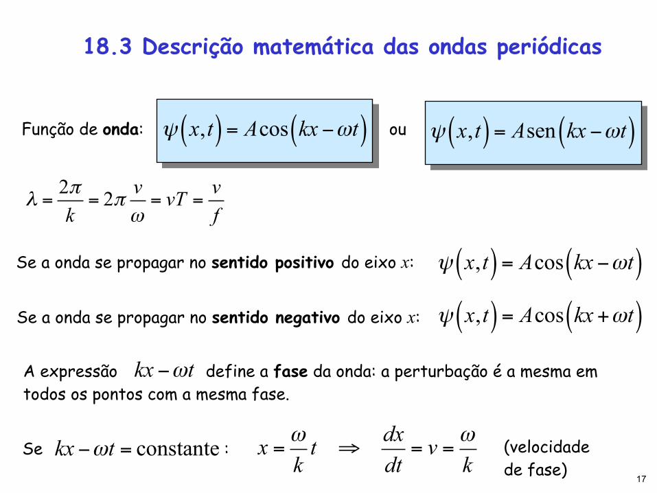
Função de onda: ou

Se a onda se propagar no sentido positivo do eixo x:

ψ x,t( ) = Asen kx −ωt( )

λ =2πk= 2π v

ω= vT = v

f

ψ x,t( ) = Acos kx −ωt( )

Se a onda se propagar no sentido negativo do eixo x:

ψ x,t( ) = Acos kx −ωt( )ψ x,t( ) = Acos kx +ωt( )

A expressão define a fase da onda: a perturbação é a mesma em todos os pontos com a mesma fase.

kx −ωt

Se : kx −ωt = constante x = ωkt ⇒

dxdt= v = ω

k(velocidade de fase)

18

A função de onda é solução da ψ x,t( ) = Acos kx −ωt( )

∂2ψ x,t( )∂x2

=1

v2∂2ψ x,t( )∂t2

equação das ondas

18.3 Descrição matemática das ondas periódicas